Complexity Analysis and DSP Implementation of the Fractional-Order Lorenz Hyperchaotic System

Abstract

The fractional-order hyperchaotic Lorenz system is solved as a discrete map by applying the Adomian decomposition method (ADM). Lyapunov Characteristic Exponents (LCEs) of this system are calculated according to this deduced discrete map. Complexity of this system versus parameters are analyzed by LCEs, bifurcation diagrams, phase portraits, complexity algorithms. Results show that this system has rich dynamical behaviors. Chaos and hyperchaos can be generated by decreasing fractional order q in this system. It also shows that the system is more complex when q takes smaller values. SE and C${}_0$ complexity algorithms provide a parameter choice criteria for practice applications of fractional-order chaotic systems. The fractional-order system is implemented by digital signal processor (DSP), and a pseudo-random bit generator is designed based on the implemented system, which passes the NIST test successfully.

1. Introduction

In recent years, dynamics of fractional-order chaotic systems have become a hot topic [1,2,3]. Secure communication and information encryption based on these fractional-order systems have also aroused people’s interests [4,5,6]. Now, three approaches are mainly derived to solve fractional-order chaotic systems: frequency-domain method [7], Adomian Decomposition Method (ADM) [8] and Adams-Bashforth-Moulton (ABM) algorithm [9]. However, Tavazoei et al. [10] reported that the frequency-domain method is not always reliable in detecting chaos behavior in nonlinear systems. On the other hand, ABM and ADM are more accurate and convenient to analyze dynamical behaviors of a nonlinear system. Compared with the ABM, ADM yields more accurate results and needs less computing resources as well as memory resources [11]. So the numerical simulations in this paper are done by applying ADM scheme.

Lyapunov Characteristic Exponents (LCEs) are necessary and more convenient for detecting hyperchaos in fractional-order hyperchaotic system. A definition of LCEs for fractional differential systems was given in Reference [12] based on frequency-domain approximations, but the limitations of frequency-domain approximations are highlighted in Reference [10]. Time series based LCEs calculation methods like Wolf algorithm [13], Jacobian method [14] and neural network algorithm [15] are associated with difficulties in choosing the embedding dimension and the delay parameter inherent of the phase-space reconstruction. Recently, LCEs of fractional-order chaotic systems are calculated based on ADM by applying QR decomposition method [16]. However, there are few references discussing LCEs of fractional-order chaotic system versus parameters and fractional order q.

Complexity measure is also an important way to analyze dynamics of a chaotic system. It can reflect the security of the system to some extent, if it is used in information security. Currently, there are several methods to measure complexity of time series, including permutation entropy (PE) [17], statistical complexity measure (SCM) [18], sample entropy (SampEn) [19], fuzzy entropy (FuzzyEn) [20], spectral entropy (SE) [21], and C${}_0$ algorithm [22]. Among them, SE and C${}_0$ algorithms are proper choices to estimate the complexity of a time series accurately and rapidly without any over-coarse graining preprocessing [21,22]. They are used to measure the complexity of chaotic systems [23,24] and physiological signals [25], respectively. However, few papers have reported complexity analysis of fractional-order chaotic systems.

In addition, compared with analog circuit implementation, digital circuit realization is a more reliable and accurate way for the application of fractional-order chaotic systems. We will also focus on the digital circuit realization of the fractional-order chaotic system.

The rest of the paper is organized as follows. In Section 2, the fractional-order Lorenz hyperchaotic system is solved numerically. In Section 3, dynamics and complexity of the system are analyzed and some interesting results are illustrated. In Section 4, the system is implemented by DSP, then a pseudo-random bit generator is designed based on the implemented system. Finally, we summarize the results.

2. Numerical Solution of the Fractional-Order Lorenz Hyperchaotic System

2.1. Adomian Decomposition Method

For a given fractional-order chaotic system with the form of ${{}^{*}D}_{t_0}^q\mathbf{x}\left(t\right)=f\left(\mathbf{x}\left(t\right)\right)$, where $\mathbf{x}\left(t\right)={[x\left(t\right),y\left(t\right),z\left(t\right),u\left(t\right)]}^T$ are the state variables. ${{}^{*}D}_{t_0}^q$ is the Caputo fractional derivative with the order $(0<q\le 1)$, and it is defined as [26]

$${{}^{*}D}_{t_0}^{q}x\left(t\right)=\left\{\begin{array}{c}\frac{1}{\mathrm{\Gamma }(1-q)}{\int }_{t_0}^t\frac{\dot{x}\left(\mathsf{\tau }\right)}{{(t-\mathsf{\tau })}^q}d\mathsf{\tau },0<q<1\hfill \\ \frac{dx\left(t\right)}{dt},q=1\hfill \end{array}\right..$$

(1)

This system can be separated into two parts as following form

$$\left\{\begin{array}{c}{{}^{*}D}_{t_0}^q\mathbf{x}\left(t\right)=L\mathbf{x}\left(t\right)+N\mathbf{x}\left(t\right)\hfill \\ {\mathbf{x}}^{\left(k\right)}\left(t_0^{+}\right)={\mathbf{b}}_k,k=0,...,m-1\hfill \end{array}\right..$$

(2)

Here, $m=ceil\left(q\right)$, ${\mathbf{b}}_k$ is a specified constant relating to the initial values, and $L\mathbf{x}\left(t\right)$ and $N\mathbf{x}\left(t\right)$ are the linear and nonlinear terms of the fractional differential equations respectively. By applying the R-L fractional integral operator to both sides of Equation (2), the following equation is obtained [26,27]

$$\mathbf{x}=J_{t_0}^{q}L\mathbf{x}+J_{t_0}^{q}N\mathbf{x}+\sum _{k=0}^{m-1}{\mathbf{b}}_k\frac{{(t-t_0)}^k}{k!},$$

(3)

where the definition of R-L fractional-order integral operator $J_{t_0}^q$ is [26]

$$J_{t_0}^{q}x\left(t\right)=\frac{1}{\mathrm{\Gamma }\left(q\right)}{\int }_{t_0}^t{(t-\mathsf{\tau })}^{q-1}x\left(\mathsf{\tau }\right)d\mathsf{\tau }.$$

(4)

According to [27], the nonlinear terms can be evaluated by

$$\left\{\begin{array}{c}{A}^i({\mathbf{x}}^0,{\mathbf{x}}^1,...,{\mathbf{x}}^i)=\frac{1}{i!}{[\frac{d^i}{d{\mathsf{\lambda }}^i}N\left({\nu }^i\left(\mathsf{\lambda }\right)\right)]}_{\mathsf{\lambda }=0}\hfill \\ {\nu }^i\left(\mathsf{\lambda }\right)=\sum _{k=0}^i{\left(\mathsf{\lambda }\right)}^k{\mathbf{x}}^k\hfill \end{array}\right.,$$

(5)

where $i=0,1,...,\infty$. Then the nonlinear terms are expressed as

$$N\mathbf{x}=\sum _{i=0}^{\infty }{\mathbf{A}}^i({\mathbf{x}}^0,{\mathbf{x}}^1,...,{\mathbf{x}}^i).$$

(6)

According to Reference [8], the solution of Equation (2) is derived by

$$\left\{\begin{array}{c}{\mathbf{x}}^0=\sum _{k=0}^{m-1}{\mathbf{b}}_k\frac{{(t-t_0)}^k}{k!}\hfill \\ {\mathbf{x}}^1=J_{t_0}^{q}L{\mathbf{x}}^0+J_{t_0}^q{\mathbf{A}}^0\left({\mathbf{x}}^0\right)\hfill \\ {\mathbf{x}}^2=J_{t_0}^{q}L{\mathbf{x}}^1+J_{t_0}^q{\mathbf{A}}^1({\mathbf{x}}^0,{\mathbf{x}}^1)\hfill \\ \text{...}\hfill \\ {\mathbf{x}}^i=J_{t_0}^{q}L{\mathbf{x}}^{i-1}+J_{t_0}^q{\mathbf{A}}^{i-1}({\mathbf{x}}^0,{\mathbf{x}}^1,...,{\mathbf{x}}^{i-1})\hfill \\ \text{...}\hfill \end{array}\right..$$

(7)

The analytical solution of the fractional-order system is presented by

$$\mathbf{x}\left(t\right)=\sum _{i=0}^{\infty }{\mathbf{x}}^i=F\left(\mathbf{x}\left(t_0\right)\right).$$

(8)

Because ADM converges fast [11,16], the first 6 terms are used to get the solution of system (2). In the real cases, it is impossible to estimate the high accuracy value of $\mathbf{x}$ when t takes large value. So, it is necessary to design a time discretization method. That is to say, for a time interval $[t_0,t]$, we divide the interval into subintervals $[t_n,t_{n+1}]$. Then we get the value of $\mathbf{x}\left(t_{n+1}\right)$ based on $\mathbf{x}\left(t_n\right)$ by applying function $F(·)$. Finally, the numerical solution of the fractional-order chaotic system are denoted as a discrete map $\mathbf{x}(n+1)=F\left(\mathbf{x}\right(n\left)\right)$.

2.2. Fractional-Order Lorenz Hyperchaotic System

By introducing a nonlinear quadratic controller u to the second equation of Lorenz system, a four dimensional dynamic system is obtained [28]

$$\left\{\begin{array}{c}\dot{x}=10(y-x)\hfill \\ \dot{y}=28x-xz+y-u\hfill \\ \dot{z}=xy-\frac{8}{3}z\hfill \\ \dot{u}=kyz\hfill \end{array}\right.,$$

(9)

where $k(0<k\le 1)$ is a parameter. When $k\in (0,0.152)$, the system is a hyperchaotic system. When $k\in$ [0.152, 0.21)∪[0.34,0.49), the system (9) is chaotic, and the system undergoes periodic orbits for the rest region of k [28]. By introducing fractional derivative to this system, the fractional-order Lorenz hyperchaotic is obtained

$$\left\{\begin{array}{c}{{}^{*}D}_{t_0}^{q}x=10(y-x)\hfill \\ {{}^{*}D}_{t_0}^{q}y=28x-xz+y-u\hfill \\ {{}^{*}D}_{t_0}^{q}z=xy-\frac{8}{3}z\hfill \\ {{}^{*}D}_{t_0}^{q}u=kyz\hfill \end{array}\right..$$

(10)

Here, the fractional-order system is solved by ADM. By introducing some intermediate variables, a rapid iteration scheme of the fractional-order hyperchaotic Lorenz system is obtained. It is shown as

$$\left\{\begin{array}{c}{x}_{n+1}={\sum }_{j=0}^6{K}_1^j{h}^{jq}/\mathrm{\Gamma }(jq+1)\hfill \\ y_{n+1}={\sum }_{j=0}^6{K}_2^j{h}^{jq}/\mathrm{\Gamma }(jq+1)\hfill \\ z_{n+1}={\sum }_{j=0}^6{K}_3^j{h}^{jq}/\mathrm{\Gamma }(jq+1)\hfill \\ u_{n+1}={\sum }_{j=0}^6{K}_4^j{h}^{jq}/\mathrm{\Gamma }(jq+1)\hfill \end{array}\right..$$

(11)

The intermediate variables $K_i^j(i=1,...,4,j=0,1,...,6)$ are shown as follows.

$$K_1^0=x_n,K_2^0=y_n,K_3^0=z_n,K_4^0=u_n,$$

(12)

$$\left\{\begin{array}{c}{K}_1^1=10(K_2^0-K_1^0)\hfill \\ K_2^1=28K_1^0-K_1^0{K}_3^0+K_2^0-K_4^0\hfill \\ K_3^1=K_1^0{K}_2^0-\frac{8}{3}{K}_3^0\hfill \\ K_4^1=k{K}_2^0{K}_3^0\hfill \end{array}\right.,$$

(13)

$$\left\{\begin{array}{c}{K}_1^2=10(K_2^1-K_1^1)\hfill \\ K_2^1=28K_1^1-K_1^1{K}_3^0-K_1^0{K}_3^1+K_2^1-K_4^1\hfill \\ K_3^2=K_1^1{K}_2^0+K_1^0{K}_2^1-\frac{8}{3}{K}_3^1\hfill \\ K_4^2=k(K_2^1{K}_3^0+K_2^0{K}_3^1)\hfill \end{array}\right.,$$

(14)

$$\left\{\begin{array}{c}{K}_1^3=10(K_2^2-K_1^2)\hfill \\ K_2^3=28K_1^2-K_1^0{K}_3^2-\frac{\mathrm{\Gamma }(2q+1)}{{\mathrm{\Gamma }}^2(q+1)}{K}_1^1{K}_3^1-K_1^2{K}_3^0+K_2^2-K_4^2\hfill \\ K_3^3=K_1^0{K}_2^2+\frac{\mathrm{\Gamma }(2q+1)}{{\mathrm{\Gamma }}^2(q+1)}{K}_1^1{K}_2^1+K_1^2{K}_2^0-\frac{8}{3}{K}_3^2\hfill \\ K_4^3=k[K_2^0{K}_3^2+\frac{\mathrm{\Gamma }(2q+1)}{{\mathrm{\Gamma }}^2(q+1)}{K}_2^1{K}_3^1+K_2^2{K}_3^0]\hfill \end{array}\right.,$$

(15)

$$\left\{\begin{array}{c}{K}_1^4=10(K_2^3-K_1^3)\hfill \\ K_2^4=28K_1^3-K_1^0{K}_3^3-K_1^3{K}_3^0+K_2^3-K_4^3-\frac{\mathrm{\Gamma }(3q+1)}{\mathrm{\Gamma }(q+1)\mathrm{\Gamma }(2q+1)}(K_1^1{K}_3^2+K_1^2{K}_3^1)\hfill \\ K_3^4=K_1^0{K}_2^3+\frac{\mathrm{\Gamma }(3q+1)}{\mathrm{\Gamma }(q+1)\mathrm{\Gamma }(2q+1)}(K_1^2{K}_2^1+K_1^1{K}_2^2)+K_1^3{K}_2^0-\frac{8}{3}{K}_3^3\hfill \\ K_4^4=k[K_2^0{K}_3^3+\frac{\mathrm{\Gamma }(3q+1)}{\mathrm{\Gamma }(q+1)\mathrm{\Gamma }(2q+1)}(K_2^2{K}_3^1+K_2^1{K}_3^2)+K_2^3{K}_3^0]\hfill \end{array}\right.,$$

(16)

$$\left\{\begin{array}{c}{K}_1^5=10(K_2^4-K_1^4)\hfill \\ K_2^5=28K_1^4-K_1^0{K}_3^4-K_1^4{K}_3^0+K_2^4-K_4^4-\frac{\mathrm{\Gamma }(4q+1)}{\mathrm{\Gamma }(q+1)\mathrm{\Gamma }(3q+1)}(K_1^1{K}_3^3+K_1^3{K}_3^1)-\hfill \\ \frac{\mathrm{\Gamma }(4q+1)}{{\mathrm{\Gamma }}^2(2q+1)}{K}_1^2{K}_3^2\hfill \\ K_3^5=K_1^0{K}_2^4+\frac{\mathrm{\Gamma }(4q+1)}{\mathrm{\Gamma }(q+1)\mathrm{\Gamma }(3q+1)}(K_1^1{K}_2^3+K_1^3{K}_2^1)+\frac{\mathrm{\Gamma }(4q+1)}{{\mathrm{\Gamma }}^2(2q+1)}{K}_1^2{K}_2^2+\hfill \\ K_1^0{K}_2^4-\frac{8}{3}{K}_3^4\hfill \\ K_4^5=k[K_2^0{K}_3^4+\frac{\mathrm{\Gamma }(4q+1)}{\mathrm{\Gamma }(q+1)\mathrm{\Gamma }(3q+1)}(K_2^1{K}_3^3+K_2^3{K}_3^1)+\frac{\mathrm{\Gamma }(4q+1)}{{\mathrm{\Gamma }}^2(2q+1)}{K}_2^2{K}_3^2+K_2^0{K}_3^4]\hfill \end{array}\right.,$$

(17)

$$\left\{\begin{array}{c}{K}_1^6=10(K_2^5-K_1^5)\hfill \\ K_2^6=28K_1^5-K_1^0{K}_3^5-K_1^5{K}_3^0+K_2^5-K_4^5-\frac{\mathrm{\Gamma }(5q+1)}{\mathrm{\Gamma }(q+1)\mathrm{\Gamma }(4q+1)}(K_1^1{K}_3^4+K_1^4{K}_3^1)\hfill \\ -\frac{\mathrm{\Gamma }(5q+1)}{\mathrm{\Gamma }(2q+1)\mathrm{\Gamma }(3q+1)}(K_1^2{K}_3^3+K_1^3{K}_3^2)\hfill \\ K_3^6=K_1^0{K}_2^5+\frac{\mathrm{\Gamma }(5q+1)}{\mathrm{\Gamma }(q+1)\mathrm{\Gamma }(4q+1)}(K_1^1{K}_2^4+K_1^4{K}_2^1)+\frac{\mathrm{\Gamma }(5q+1)}{\mathrm{\Gamma }(2q+1)\mathrm{\Gamma }(3q+1)}(K_1^2{K}_2^3\hfill \\ +K_1^3{K}_2^2)+K_1^5{K}_2^0-\frac{8}{3}{K}_3^5\hfill \\ K_4^6=k[K_2^0{K}_3^5+\frac{\mathrm{\Gamma }(5q+1)}{\mathrm{\Gamma }(q+1)\mathrm{\Gamma }(4q+1)}(K_2^1{K}_3^4+K_2^4{K}_3^1)+\frac{\mathrm{\Gamma }(5q+1)}{\mathrm{\Gamma }(2q+1)\mathrm{\Gamma }(3q+1)}(K_2^2{K}_3^3+\hfill \\ K_2^3{K}_3^2)+K_2^5{K}_3^0]\hfill \end{array}\right..$$

(18)

where $h=t_{m+1}-t_m$, and $\mathrm{\Gamma }(·)$ is the Gamma function. Based on the discrete map Equation (11), it is easy to get the time series by the way of computer programming. Also it provides the necessary discrete iterative equations for the fractional-order hyperchaotic Lorenz system implemented on DSP platform. In this paper, we set $h=0.01$. Dynamics under two parameters q and k are analyzed in the following sections.

3. Dynamics Analysis of the Fractional-Order Lorenz Hyperchaotic System

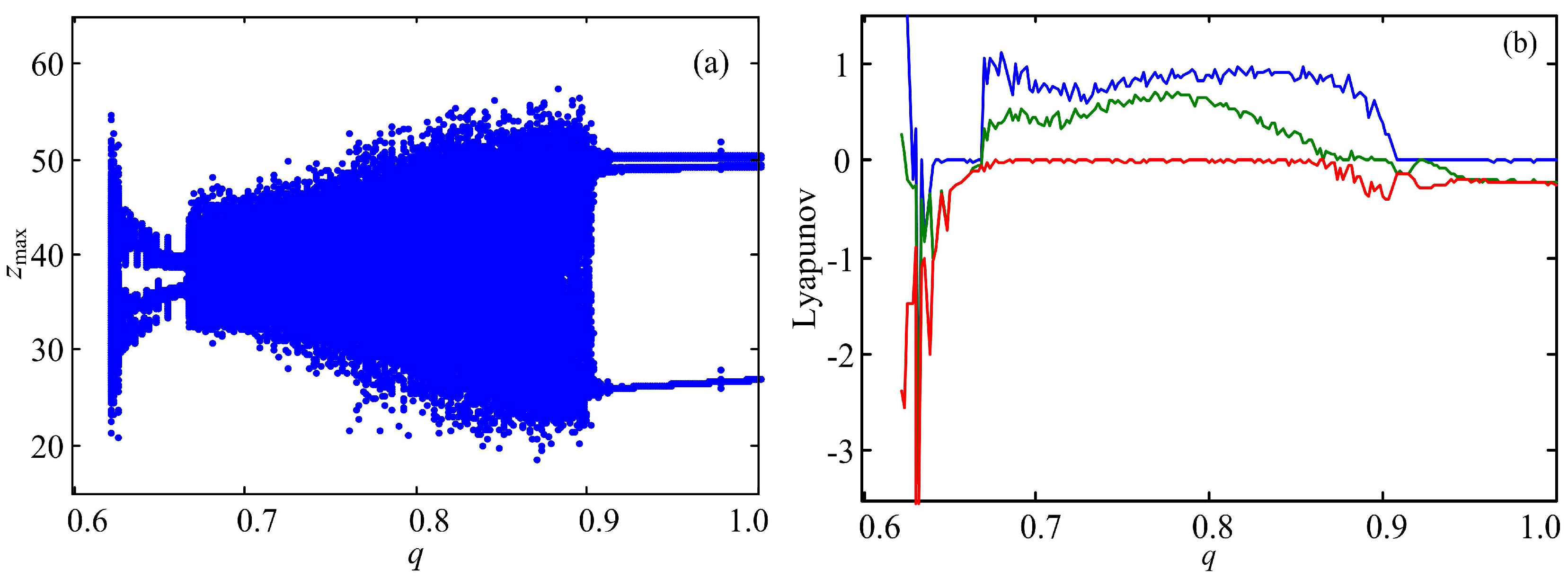
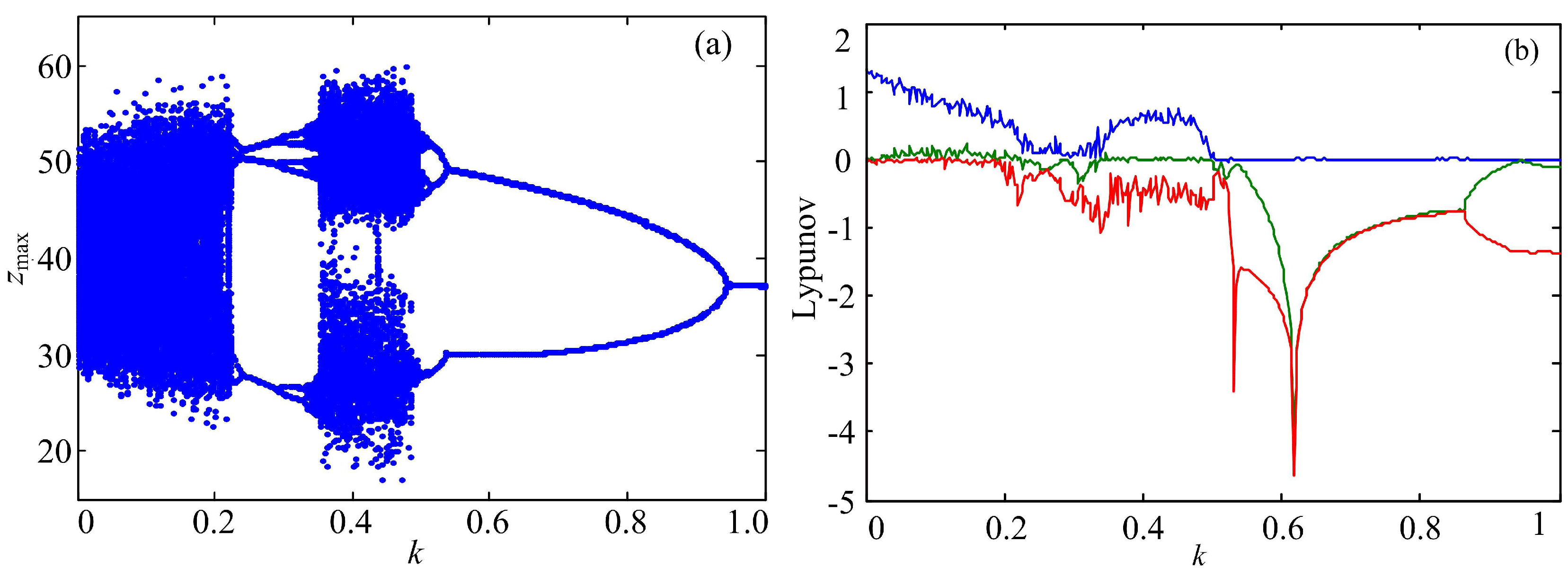
3.1. Bifurcation Analysis

For the discrete map Equation (11), LCEs can be calculated by employing QR decomposition method [16]. The computational process is shown as follows.

$$\begin{array}{cc}\hfill qr[{\mathbf{J}}_M{\mathbf{J}}_{M-1}...{\mathbf{J}}_1]& =qr[{\mathbf{J}}_M{\mathbf{J}}_{M-1}...{\mathbf{J}}_2\left({\mathbf{J}}_1{\mathbf{Q}}_0\right)]\hfill \\ & ={\mathbf{Q}}_M[{\mathbf{R}}_M...{\mathbf{R}}_2{\mathbf{R}}_1]\hfill \end{array},$$

(19)

where $qr[·]$ represents QR decomposition function, and $\mathbf{J}$ is the Jacobian matrix of the given map Equation (11). All LCEs can be calculated by

$${\mathsf{\lambda }}_k=\frac{1}{Mh}\sum _{i=1}^{M}ln\left|{\mathbf{R}}_i(k,k)\right|,$$

(20)

where $k=1,2,3,4$, and M is the maximum iteration number. Let $M=20,000$ for accurate and stable outputs. In this study, we just show the first three ${\mathsf{\lambda }}_1,{\mathsf{\lambda }}_2$ and ${\mathsf{\lambda }}_3$ for better observation as well as for legibility. LCEs and the corresponding bifurcation diagram of the fractional-order Lorenz hyperchaotic system with q varying and k varying are analyzed.

(1) Fix $k=0.26$ and vary q from 0.60 to 1.00 with the step of $\Delta q=0.001$. The bifurcation diagram and Lyapunov characteristic exponents are shown in Figure 1. It illustrates that the states of the system are different as q increases. The period windows are observed at $q\in [0.6340,0.6700]\cup (0.906,1]$. When $q\in (0.670,0.860]$, the system is a hyperchaotic system. When $q\in (0.860,0.906]$, this system is chaotic. It is worth pointing out that the periodic state of the integer order system becomes chaotic or hyperchaotic when order q changes to fractional order.

Figure 1. Bifurcation and Lyapunov Characteristic Exponents (LCEs) with different q ($k=0.26$) (a) Bifurcation diagram; (b) Lyapunov characteristic exponents.

Figure 1. Bifurcation and Lyapunov Characteristic Exponents (LCEs) with different q ($k=0.26$) (a) Bifurcation diagram; (b) Lyapunov characteristic exponents.

(2) Fix $q=0.96$ and vary k from 0 to 1 with the step of $\Delta k=0.0025$. The bifurcation diagram and Lyapunov characteristic exponents are shown in Figure 2. It illustrates that the system is hyperchaotic at $k\in (0,0.1875]$. When $k\in (0.1875,0.2275]\cup (0.3400,0.4975]$, the system is in chaotic state, and it is periodic for $k\in (0.2275,0.3400]\cup (0.4975,1]$.

Figure 2. Bifurcation and LCEs with different k ($q=0.96$) (a) Bifurcation diagram; (b) Lyapunov characteristic exponents.

Figure 2. Bifurcation and LCEs with different k ($q=0.96$) (a) Bifurcation diagram; (b) Lyapunov characteristic exponents.

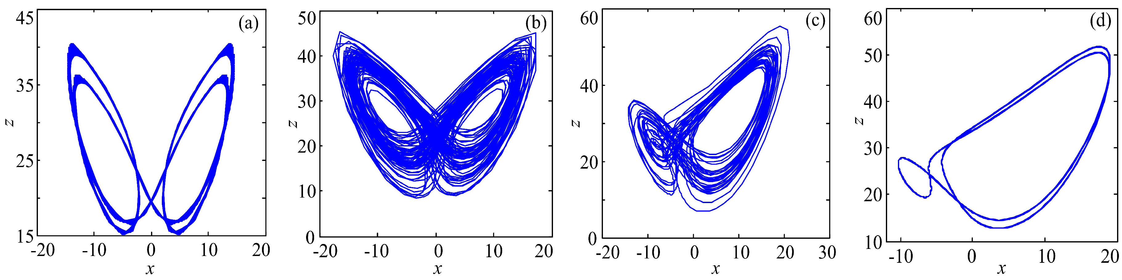
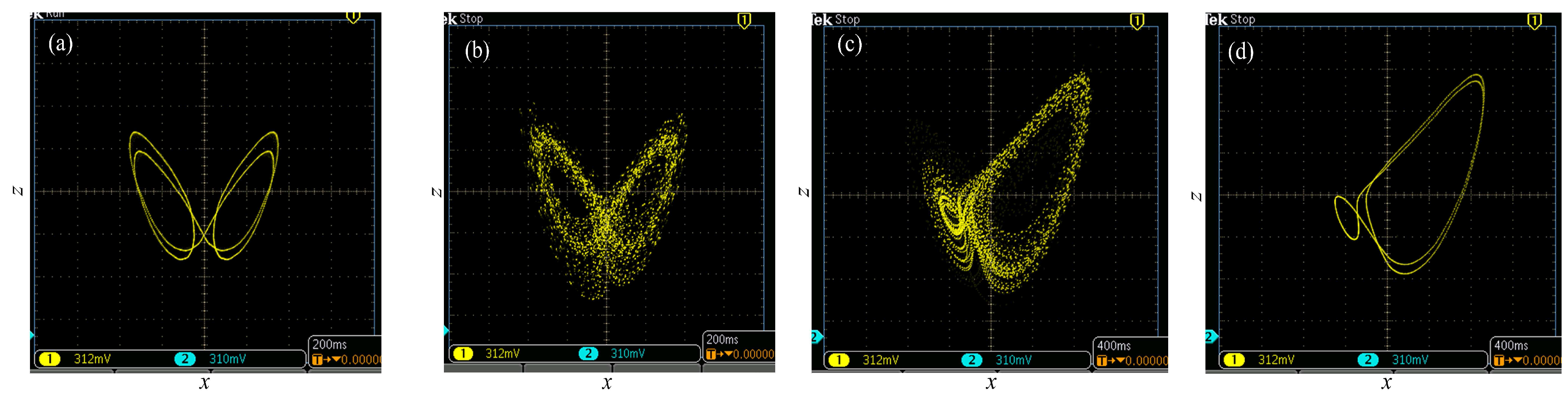
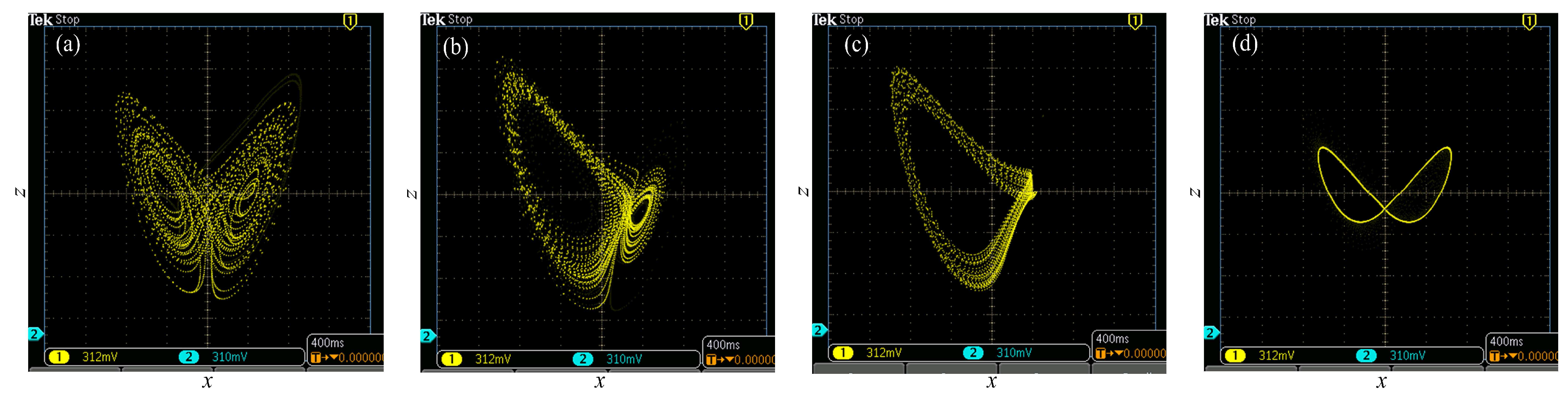
3.2. Observation of Chaotic Attractors

To further observe the dynamical behavior, some typical chaotic attractors of system (10) are recorded according to the bifurcation analysis results above. These phase portraits are shown in Figure 3 and Figure 4 with $k=0.26$, q varying and $q=0.96$, k varying, respectively.

Results with $k=0.26$ and q varying are summarized as follows. (1) The system is periodic when $q=0.65$ as shown in Figure 3a; (2) The system is hyperchaotic when $q=0.72$ as shown in Figure 3b, and the attractor has two wings; (3) The system is chaotic when $q=0.89$ as shown in Figure 3c, which is different from the above two attractors; (4) The system is periodic when $q=1.00$ as shown in Figure 3d. It is interesting that this fractional-order system generates chaos and hyperchaos, while its integer-order counterpart is non-chaotic.

Figure 3. Phase diagrams of fractional-order hyperchaotic Lorenz system ($k=0.26$) (a) periodic orbits ($q=0.65$); (b) hyperchaos ($q=0.72$); (c) chaos ($q=0.89$); (d) periodic orbits ($q=1.00$).

Figure 3. Phase diagrams of fractional-order hyperchaotic Lorenz system ($k=0.26$) (a) periodic orbits ($q=0.65$); (b) hyperchaos ($q=0.72$); (c) chaos ($q=0.89$); (d) periodic orbits ($q=1.00$).

Results with $q=0.96$ and k varying are summarized as follows. (1) When $k=0.0.05$, the hyperchaos strange attractor is shown in Figure 4a, the attractor is similar with the hyperchaos strange attractor in Figure 3a; (2) When $k=0.20$, the chaos attractor is shown in Figure 4b, a typical chaotic attractor of this system; (3) When $k=0.25$, the periodic orbits is shown in Figure 4c; (4) When $k=0.30$, the periodic orbits is shown in Figure 4d; (5) When $k=0.40$, the chaos attractor is shown in Figure 4e; (6) When $k=0.50$, a quasi-periodic orbits is shown in Figure 4f; (7) When $k=0.80$, the periodic orbits is shown in Figure 4g; (8) When $k=1.00$, the periodic orbits is shown in Figure 4h, it is different from those in the above situations.

Figure 4. Phase diagrams of fractional-order hyperchaotic Lorenz system $(q=0.96)$ (a) hyperchaos ($k=0.05$); (b) chaos ($k=0.20$); (c) periodic orbits ($k=0.25$); (d) periodic orbits ($k=0.30$); (e) chaos ($k=0.40$); (f) quasi-periodic orbits ($k=0.50$); (g) periodic orbits ($k=0.80$); (h) periodic orbits ($k=1.00$).

Figure 4. Phase diagrams of fractional-order hyperchaotic Lorenz system $(q=0.96)$ (a) hyperchaos ($k=0.05$); (b) chaos ($k=0.20$); (c) periodic orbits ($k=0.25$); (d) periodic orbits ($k=0.30$); (e) chaos ($k=0.40$); (f) quasi-periodic orbits ($k=0.50$); (g) periodic orbits ($k=0.80$); (h) periodic orbits ($k=1.00$).

It can be seen from the simulation results that the system undergoes hyperchaos, chaos, and some different periodic orbits when the parameter k and fractional-order q vary. Fractional order q should be treated as a bifurcation parameter as it also determines dynamics of the system. By applying ADM, the fractional-order Lorenz hyperchaotic system can be used in fields like secure communication, image encryption and digital watermark.

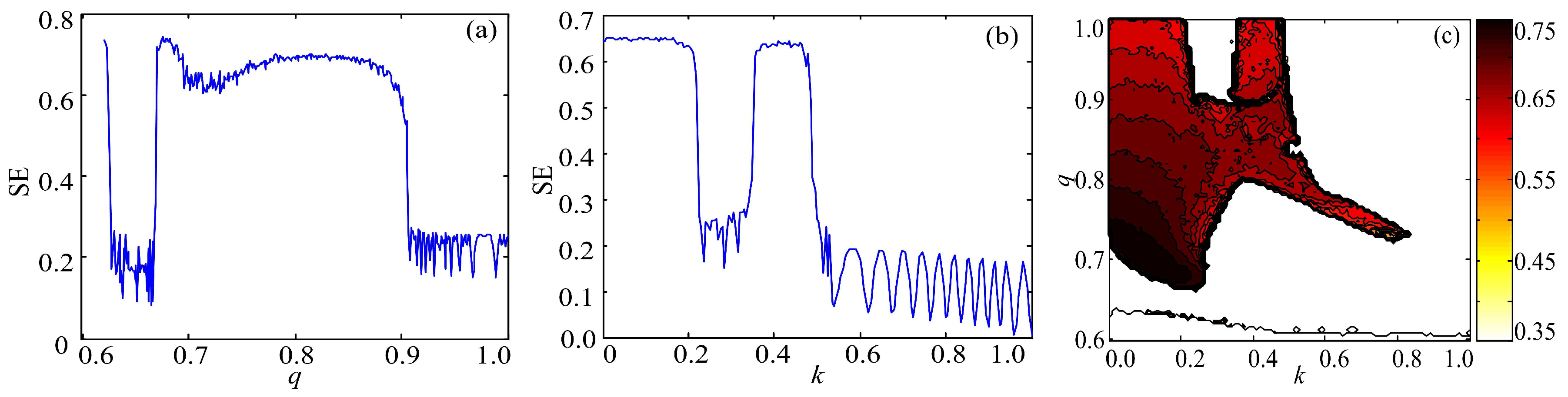
3.3. Spectral Entropy Complexity Analysis

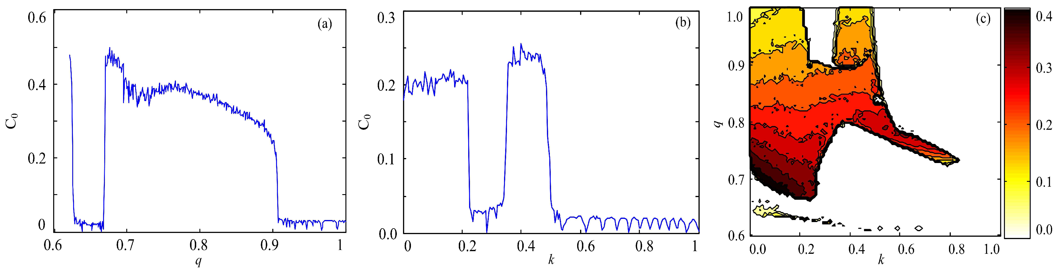
SE reflects the disorder in the Fourier transformation domain. A flatter spectrum has a larger value of SE, which shows a higher complexity of the time series. SE is described as follows. Given a time series {x(n), n = 0, 1, 2,..., $N-1$} with a length of N, let $x\left(n\right)=x\left(n\right)-\overline{x}$ , where $\overline{x}$ is the mean value of time series. Its corresponding Discrete Fourier Transformation (DFT) is defined by

$$X\left(k\right)=\sum _{n=0}^{N-1}x\left(n\right)e^{-j2\pi nk/N},$$

(21)

where $k=0,1...,N-1$ and j is the imaginary unit. If the power of a discrete power spectrum with the $k_{th}$ frequency is ${\left|X\left(k\right)\right|}^2$, then the “probability” of this frequency is defined as

$$P_k=\frac{{\left|X\left(k\right)\right|}^2}{{\sum }_{k=0}^{N/2-1}{\left|X\left(k\right)\right|}^2}.$$

(22)

When the DFT is employed, the summation runs from $k=0$ to $k=N/2-1$. The normalization entropy is denoted by [21]

$$\text{SE}=\frac{{\sum }_{k=0}^{N/2-1}\left|P_{k}ln\left(P_k\right)\right|}{ln(N/2)},$$

(23)

where $ln(N/2)$ is the entropy of completely random signal.

Complexity of x series of the fractional-order system (10) is calculated and illustrated in Figure 5. The length N for SE is 4 × 10${}^4$ after removing the first ${10}^4$ points of data. It shows in Figure 5 that the SE complexity agrees well with bifurcation results in Figure 1 and Figure 2. Thus, it is a faster and more convenient way for dynamics analysis of fractional-order chaotic system. Compared with complexity versus a parameter, complexity in the parameter plane can show us more information of the system. SE complexity in the $q-k$ parameter plane is calculated and shown in Figure 5c. It shows that complexity of the fractional-order chaotic system decreases as fractional order q increases when k is smaller than 0.2. When k is larger than 0.9, there is no chaos or hyperchaos generated for this system. Overall, high complexity region takes up about 40 percent of total parameter plane. As the SE algorithm estimates complexity very fast and illustrates the dynamics of the fractional-order chaotic system, complexity analysis is a practical basis for parameter choice in real applications.

Figure 5. Spectral entropy (SE) complexity results (a) SE complexity versus fractional order q (k = 0.26); (b) SE complexity versus fractional order k (q = 0.96); (c) SE complexity in the $q-k$ parameter plane.

Figure 5. Spectral entropy (SE) complexity results (a) SE complexity versus fractional order q (k = 0.26); (b) SE complexity versus fractional order k (q = 0.96); (c) SE complexity in the $q-k$ parameter plane.

3.4. C${}_0$ Complexity Analysis

C${}_0$ complexity is also based on the DFT, but it reflects the ratio of irregular in the series. The corresponding DFT process of the time series {x(n), n = 0, 1, 2, ..., $N-1$} is shown as formula (21). Define the mean square value of $X\left(k\right)$ as

$$G_N=(1/N)\sum _{k=0}^{N-1}|X\left(k\right){|}^2.$$

(24)

Let

$$\tilde{X}\left(k\right)=\left\{\begin{array}{c}\begin{array}{cc}X\left(k\right)& if|X\left(k\right){|}^2>r{G}_N\end{array}\hfill \\ \begin{array}{ccc}0& & if|X\left(k\right){|}^2\le r{G}_N\end{array}\hfill \end{array}\right.,$$

(25)

where r ($r>0$) is the control parameter. The inverse Fourier Transformation of $X\left(k\right)$ is

$$\tilde{x}\left(n\right)=(1/N)\sum _{k=0}^{N-1}\tilde{X}\left(k\right)e^{j2\pi nk/N},$$

(26)

where $n=0,1,...,N-1$. Finally, the C${}_0$ complexity [22] is defined as

$${\mathrm{C}}_0(r,N)=\frac{\sum _{n=0}^{N-1}|x\left(n\right)-\tilde{x}\left(n\right){|}^2}{\sum _{n=0}^{N-1}|x\left(n\right){|}^2}.$$

(27)

In this paper, we set $r=15$ to calculate the C${}_0$ complexity.

C${}_0$ complexity of x series of the fractional-order system (10) is calculated as shown in Figure 6. The data applied for complexity calculation is the same as above. According to Figure 6, C${}_0$ complexity is consistent with SE complexity as shown in Figure 5. As C${}_0$ algorithm is also fast at complexity estimation, thus it can be employed to analyze dynamics and complexity of fractional-order Lorenz hyperchaotic system. It shows that C${}_0$ algorithm provides a parameter selection method for a fractional-order Lorenz hyperchaotic system in practical application.

Figure 6. C${}_0$ complexity results (a) C${}_0$ complexity versus fractional order q (k = 0.26); (b) C${}_0$ complexity versus fractional order k (q = 0.96); (c) C${}_0$ complexity in the $q-k$ parameter plane.

Figure 6. C${}_0$ complexity results (a) C${}_0$ complexity versus fractional order q (k = 0.26); (b) C${}_0$ complexity versus fractional order k (q = 0.96); (c) C${}_0$ complexity in the $q-k$ parameter plane.

4. Digital Circuit Implementation

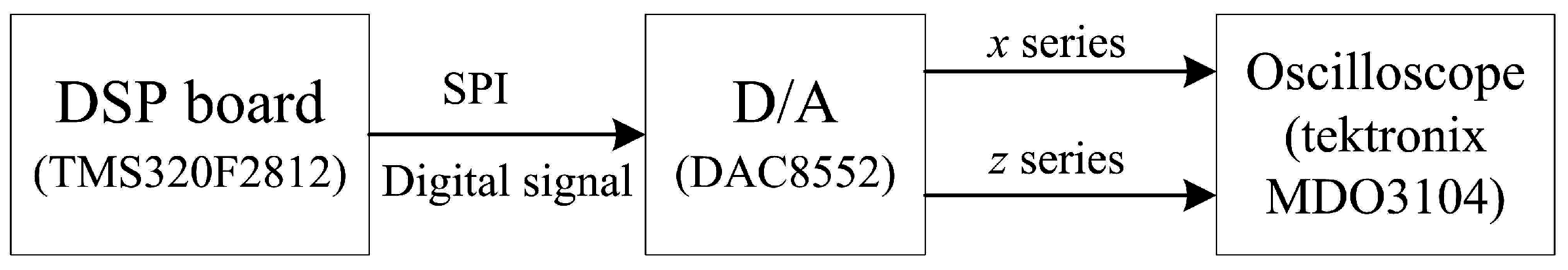
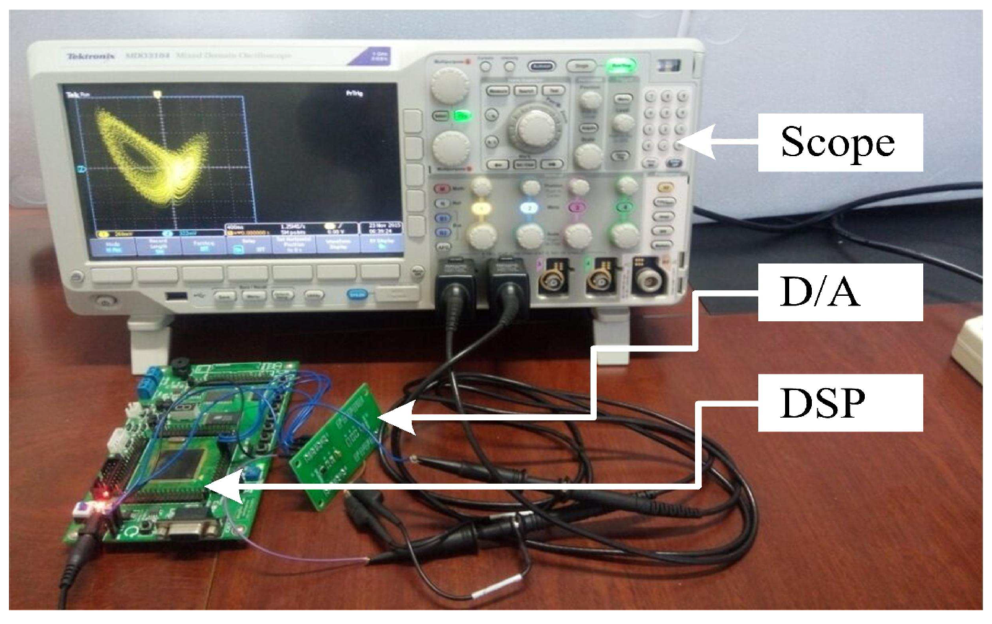
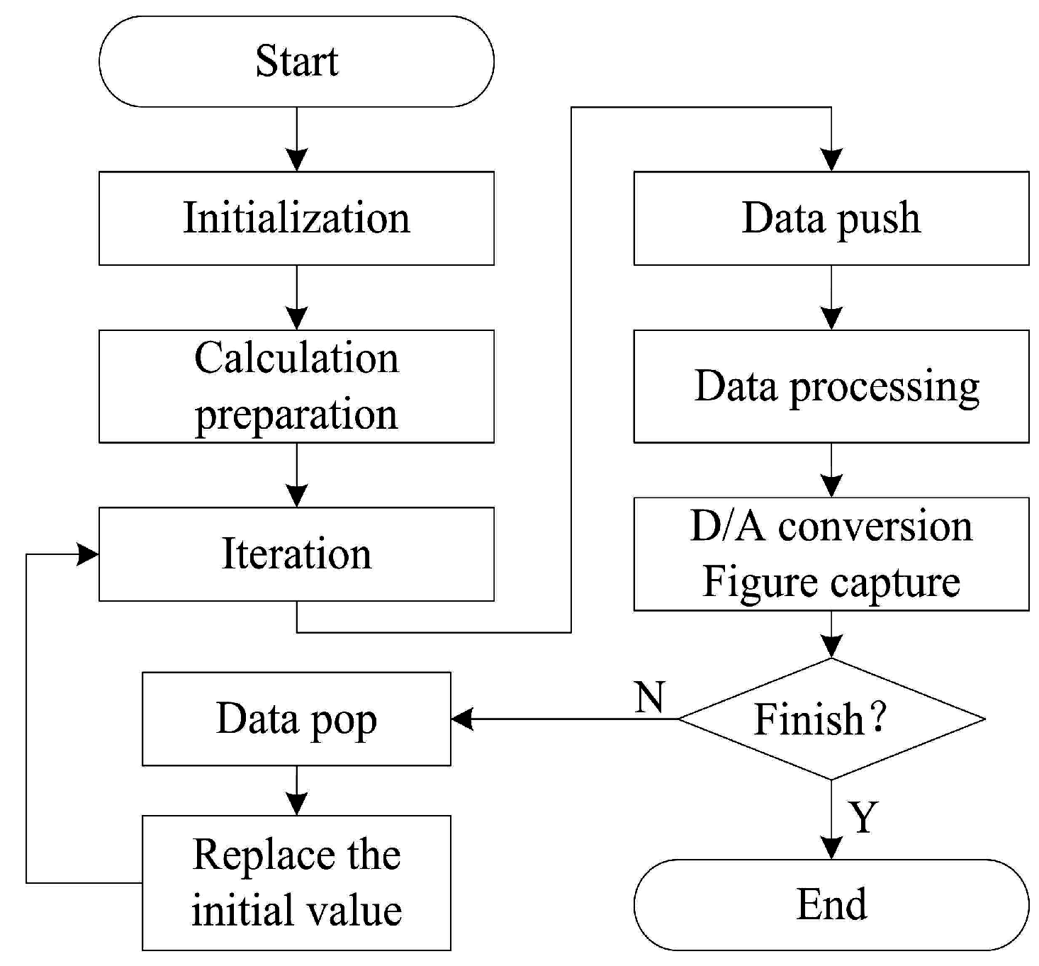
4.1. DSP Implementation

In this section, the digital circuit of the fractional-order Lorenz hyperchaotic system is implemented based on DSP technology. A hardware block diagram of the digital circuit is shown in Figure 7, and the DSP board used to perform digital implementation is shown in Figure 8. The DSP board is chosen for its powerful computing ability, and the key chip in this board is the fixed-point DSP TMS320F2812. A 16-bit dual-channel DA converter DAC8552 is used to convert time series generated by DSP. It is controlled by the DSP development board via a SPI interface. Then the converted data is sent to a oscilloscope (tektronix MDO3104) which is used to record phase portraits of the system.

Figure 7. Hardware block diagram.

Figure 7. Hardware block diagram.

Figure 8. Digital signal processor (DSP) board used to perform digital implementation.

Figure 8. Digital signal processor (DSP) board used to perform digital implementation.

The flow diagram for DSP implementation of the fractional-order system is shown in Figure 9, and Equation (11) provides a necessary iterative algorithm for the fractional-order Lorenz hyperchaotic system. C language is used to realized the discrete iterative equation and then the program is downloaded to the DSP board. To improve the iteration speed, we use a function to calculate some items like $h^q$, $\mathrm{\Gamma }(q+1)$, $h^q/\mathrm{\Gamma }(q+1)$, $h^{2q}$, $\mathrm{\Gamma }(2q+1)$, $h^{2q}/\mathrm{\Gamma }(2q+1)$ and so on in Equations (15)–(18) before iteration. In the step of data processing, all data is converted to analog signals. To reduce the impact of the data processing on the iterative computation, the operations of pushing and popping are introduced. This means that values of the state variables are placed and protected at a location pointed to a stack pointer. In a real world application, proper parameter q and k can be chosen based on the above complexity results or bifurcation results.

Figure 9. Flow diagram for DSP implementation of the fractional-order system.

Figure 9. Flow diagram for DSP implementation of the fractional-order system.

To compare computer simulation results with digital circuit simulation results, we set the simulation parameter $k=0.26$ and vary q (q = 0.65, 0.72, 0.89, and 1.00) as previously mentioned, then $x-z$ phase diagrams are shown in Figure 10. We also set q = 0.96 and vary k (k = 0.05, 0.20, 0.50, and 1.00), and $x-z$ phase diagrams are shown in Figure 11. It shows in Figure 10 and Figure 11 that phase diagrams of fractional-order Lorenz hyperchaotic system by DSP consist with the computer simulation results. In conclusion, the fractional-order hyperchaotic Lorenz system is implemented in the digital circuit.

Figure 10. Phase diagrams of the fractional-order Lorenz hyperchaotic system by DSP $(k=0.26)$ (a) periodic orbits ($q=0.65$); (b) hyperchaos ($q=0.72$); (c) chaos ($q=0.89$); (d) periodic orbits ($q=1.00$).

Figure 10. Phase diagrams of the fractional-order Lorenz hyperchaotic system by DSP $(k=0.26)$ (a) periodic orbits ($q=0.65$); (b) hyperchaos ($q=0.72$); (c) chaos ($q=0.89$); (d) periodic orbits ($q=1.00$).

Figure 11. Phase diagrams of the fractional-order Lorenz hyperchaotic system by DSP $(q=0.96)$ (a) hyperchaos ($k=0.05$); (b) chaos ($k=0.20$); (c) quasi-periodic orbits ($k=0.50$); (d) periodic orbits ($k=1.00$).

Figure 11. Phase diagrams of the fractional-order Lorenz hyperchaotic system by DSP $(q=0.96)$ (a) hyperchaos ($k=0.05$); (b) chaos ($k=0.20$); (c) quasi-periodic orbits ($k=0.50$); (d) periodic orbits ($k=1.00$).

4.2. Pseudo-Random Sequence Generator

In this section, a pseudo-random bit generator is designed and implemented on DSP board. Firstly, the coding algorithm for the pseudo-random bit generator on DSP is described as:

(1) Set $n=1$, $k=0.26$, $q=0.7$, the initial value ${\mathbf{x}}_0=[1,2,3,4]$, $M=0.125\times {10}^8+100$, and iterate the Equation (11) 1000 times. Let $n=1001$, thus ${\mathbf{x}}_0=[x\left(n\right),y\left(n\right),z\left(n\right),u\left(n\right)]$.

(2) Iterate the Equation (11) once then obtain the new value of $data=x(n+1)$ for further calculation

$$data=round\left(data\times {10}^{11}\right).$$

(28)

Thus $data$ can be expressed as a 64-bit binary number DB${}_{63}$-DB${}_0$.

(3) Define $dat{a}_1$ = DB${}_7$-DB${}_0$. Then the bit sequences $dat{a}_1$ is sent to a personal computer by the serial communication interface (SCI) and MAX3232 (RS-232 transceiver).

(4) Set $n=n+1$ and ${\mathbf{x}}_0=[x\left(n\right),y\left(n\right),z\left(n\right),u\left(n\right)]$.

(5) Do steps (2)–(4) in a loop until $n>M$.

By applying the coding algorithm, we can obtain a pseudo-random bit sequence in a computer for further statistical test. Among the numerous standard tests for pseudo-random sequences, we choose the statistical test suite of NIST to test the generated bit sequence. The suite used is the sts-2.1.2, which is available in Reference [29]. There are two indicators, namely, the uniformity of p-values and the proportion of passing sequences determining whether a PRBG passes the standard test. Here, the minimum uniformity of p-value is $0.0001$. If all p-values are larger than 0.0001 and the confidence interval satisfies

$$\left[(1-\alpha )-3\sqrt{\frac{(1-\alpha )\alpha }{m}},\left.(1-\alpha )+3\sqrt{\frac{(1-\alpha )\alpha }{m}}\right]\right.,$$

(29)

where m is the sample size and α is the the given significance level, then the pseudo-random bit generator passes the test successfully. More details about tests in NIST can be found in Reference [30].

The length of the pseudo-random bit sequence is ${10}^6$ bits, and 100 such sequences are tested. If $\alpha =0.01$, then the confidence interval is $[96.015\%,1]$ for most tests. The test result is illustrated in Table 1. For some items tested more than once (for example, N.O.Temp. is tested 148 times), we only illustrate the worst results. It shows that all p-values are larger than 0.0001 and the computed proportion for each test lies inside the confidence interval. Hence the tested binary sequences generated by the proposed pseudo-random bit generator are random.

Table 1. Nist test result of the pseudo-random bit generator.

	p-Value	Proportion	Success
Frequency	0.366918	100%	√
B. Frequency	0.002559	99%	√
C. Sums	0.275709	99%	√
Runs	0.048716	98%	√
Longest Run	0.935716	99%	√
Rank	0.883171	99%	√
FFT	0.574903	100%	√
N.O.Temp.	0.002203	97%	√
O.Temp.	0.834308	100%	√
Universal	0.759756	99%	√
App. Entropy	0.759756	98%	√
R.Excur.	0.005166	96.7%	√
R.Excur.V.	0.105618	96.7%	√
Serial	0.075719	99%	√
L. Complexity	0.554420	99%	√

Table 1. Nist test result of the pseudo-random bit generator.

	p-Value	Proportion	Success
Frequency	0.366918	100%	√
B. Frequency	0.002559	99%	√
C. Sums	0.275709	99%	√
Runs	0.048716	98%	√
Longest Run	0.935716	99%	√
Rank	0.883171	99%	√
FFT	0.574903	100%	√
N.O.Temp.	0.002203	97%	√
O.Temp.	0.834308	100%	√
Universal	0.759756	99%	√
App. Entropy	0.759756	98%	√
R.Excur.	0.005166	96.7%	√
R.Excur.V.	0.105618	96.7%	√
Serial	0.075719	99%	√
L. Complexity	0.554420	99%	√

Currently, based on DSP/FPGA technology, chaos-based applications are widely used in the engineering fields, especially in image encryption [31] and secret communication [32]. In these applications, the pseudo-random bit generator usually plays an important role. Moreover, it shows in this paper that the fractional-order chaotic systems can be used in the engineering fields.

5. Conclusions

The dynamics of the fractional-order Lorenz hyperchaotic system is investigated in this paper. It is solved as a discrete map by applying ADM. The algorithm used to calculate LCEs of the fractional-order chaotic system is presented based on the discrete map and QR decomposition algorithm. Dynamics of the fractional-order Lorenz hyperchaotic system are analyzed by means of LCEs, bifurcation diagram, phase diagram, SE and C${}_0$ complexity algorithms. Finally, the system is implemented in the digital circuit. The conclusions are drawn as follows.

(1) This fractional-order Lorenz hyperchaotic system contains rich dynamical behaviors. It is interesting that the system with integer-order is periodic, but chaos and hyperchaos are observed with the decrease of the fractional-order q.

(2) SE and C${}_0$ complexities agree well with LCEs and bifurcation diagram results. It shows that complexity analysis is a more convenient method to choose parameters of fractional-order chaotic system in the real applications. We also find that the complexity of this system decreases when q increases.

(3) The fractional-order Lorenz hyperchaotic system is implemented on DSP digital circuit. According to the implemented fractional-order system, a DSP-based pseudo-random bit generator is designed, which passes the NIST test successfully. Our further work will focus on the information encryption application of the fractional-order Lorenz hyperchaotic system.

References

1. Wang, Z.L.; Yang, D.S. Stability analysis for nonlinear fractional-order systems based on comparison principle. Nonlinear Dyn. 2014, 75, 387–402. [Google Scholar] [CrossRef]
2. Wang, Y.; Sun, K.H.; He, S.B.; Wang, H.H. Dynamics of fractional-order sinusoidally forced simplified Lorenz system and its synchronization. Eur. Phys. J. Special Top. 2014, 223, 1591–1600. [Google Scholar] [CrossRef]
3. Daftardar, G.V.; Bhalekar, S. Chaos in fractional ordered Liu system. Comp. Math. Appl. 2010, 59, 1117–1127. [Google Scholar] [CrossRef]
4. Chen, D.; Wu, C.; Herbert, H.C.I. Circuit simulation for synchronization of a fractional-order and integer-order chaotic system. Nonlinear Dyn. 2013, 73, 1671–1686. [Google Scholar] [CrossRef]
5. Tian, X.M.; Fei, S.M. Robust control of a class of uncertain fractional-order chaotic systems with input nonlinearity via an adaptive sliding mode technique. Entropy 2014, 16, 729–746. [Google Scholar] [CrossRef]
6. Zhang, L.G.; Yan, Y. Robust synchronization of two different uncertain fractional-order chaotic systems via adaptive sliding mode control. Nonlinear Dyn. 2014, 76, 1761–1767. [Google Scholar] [CrossRef]
7. Charef, A.; Sun, H.H.; Tsao, Y.Y. Fractal system as represented by singularity function. IEEE Trans. Auto. Contr. 1992, 37, 1465–1470. [Google Scholar] [CrossRef]
8. Adomian, G.A. Review of the decomposition method and some recent results for nonlinear equations. Math. Comp. Model. 1990, 13, 17–43. [Google Scholar] [CrossRef]
9. Sun, H.H.; Abdelwahab, A.A.; Onaral, B. Linear approximation of transfer function with a pole of fractional power. IEEE Trans. Auto. Contr. 1984, 29, 441–444. [Google Scholar] [CrossRef]
10. Tavazoei, M.S.; Haeri, M. Unreliability of frequency-domain approximation in recognizing chaos in fractional-order systems. IET Sign. Proc. 2007, 1, 171–181. [Google Scholar] [CrossRef]
11. He, S.B.; Sun, K.H.; Wang, H.H. Solving of fractional-order chaotic system based on Adomian decomposition algorithm and its complexity analyses. Acta Phys. Sin. 2014, 63, 030502. [Google Scholar]
12. Li, C.; Gong, Z.; Qian, D. On the bound of the Lyapunov exponents for the fractional differential systems. Chaos 2010, 20, 013127. [Google Scholar] [CrossRef] [PubMed]
13. Wolf, A.; Swift, J.B.; Swinney, H.L. Determining Lyapunov exponents from a time series. Phys. D Nonlinear Phenom. 1985, 16, 285–317. [Google Scholar] [CrossRef]
14. Ellner, S.; Gallant, A.R.; McCaffrey, D. Convergence rates and data requirements for Jacobian-based estimates of Lyapunov exponents from data. Phys. Lett. A 1991, 153, 357–363. [Google Scholar] [CrossRef]
15. Maus, A.; Sprott, J.C. Evaluating Lyapunov exponent spectra with neural networks. Chaos Solit. Fract. 2013, 51, 13–21. [Google Scholar] [CrossRef]
16. Caponetto, R.; Fazzino, S. An application of Adomian decomposition for analysis of fractional-order chaotic systems. Int. J. Bifur. Chaos 2013, 23, 1350050. [Google Scholar] [CrossRef]
17. Bandt, C.; Pompe, B. Permutation entropy: A natural complexity measure for time series. Phys. Rev. Lett. 2002, 88, 174102. [Google Scholar] [CrossRef] [PubMed]
18. Larrondo, H.A.; Gonzlez, C.M.; Martin, M.T. Intensive statistical complexity measure of pseudorandom number generators. Phys. A 2005, 356, 133–138. [Google Scholar] [CrossRef]
19. Wei, Q.; Liu, Q.; Fan, S.Z. Analysis of EEG via multivariate empirical mode decomposition for depth of anesthesia based on sample entropy. Entropy 2013, 15, 3458–3470. [Google Scholar] [CrossRef]
20. Chen, W.T.; Zhuang, J.; Yu, W.X. Measuring complexity using FuzzyEn, ApEn, and SampEn. Med. Eng. Phys. 2009, 31, 61–68. [Google Scholar] [CrossRef] [PubMed]
21. Phillip, P.A.; Chiu, F.L.; Nick, S.J. Rapidly detecting disorder in rhythmic biological signals: A spectral entropy measure to identify cardiac arrhythmias. Phys. Rev. E 2009, 79, 011915. [Google Scholar]
22. Shen, E.H.; Cai, Z.J.; Gu, F.J. Mathematical foundation of a new complexity measure. Appl. Math. Mech. 2005, 26, 1188–1196. [Google Scholar]
23. He, S.B.; Sun, K.H.; Zhu, C.X. Complexity analyses of multi-wing chaotic systems. Chin. Phys. B 2013, 22, 050506. [Google Scholar] [CrossRef]
24. Sun, K.H.; He, S.B.; He, Y. Complexity analysis of chaotic pseudo-random sequence based on spectral entropy algorithm. Acta Phys. Sin. 2013, 62, 010501. [Google Scholar]
25. Cao, Y.; Cai, Z.J.; Shen, E.H. Quantitative analysis of brain optical images with 2D C0 complexity measure. J. Neurosci. Meth. 2007, 159, 181–186. [Google Scholar] [CrossRef] [PubMed]
26. Cafagna, D.; Grassim, G. Bifurcation and chaos in the fractional-order Chen system via a time-domain approach. Int. J. Bifur. Chaos 2008, 18, 1845–1863. [Google Scholar] [CrossRef]
27. Shawagfeh, N.T. Analytical approximate solutions for nonlinear fractional differential equations. Appl. Math. Comp. 2002, 131, 517–529. [Google Scholar] [CrossRef]
28. Gao, T.G.; Chen, G.R.; Chen, Z.Q. The generation and circuit implementation of a new hyper-chaos based upon Lorenz system. Phys. Lett. A 2007, 361, 78–86. [Google Scholar] [CrossRef]
29. NIST Computer Security Resource Center. Available online: http://csrc.nist.gov/groups/ST/toolkit/rng/documentation_software.html (accessed on 17 December 2015).
30. Runkin, A.; Soto, J.; Nechvatal, J. A Statistical Test Suite for Random and Pseudorandom Number Generators for Cryptographic Applications. Available online: http://nvlpubs.nist.gov/nistpubs/Legacy/SP/nistspecialpublication800-22.pdf (accessed on 17 December 2015).
31. Tlelo-Cuautle, E.; Carbajal-Gomez, V.H.; Obeso-Rodelo, P.J. FPGA realization of a chaotic communication system applied to image processing. Nonlinear Dyn. 2015, 82, 1879–1892. [Google Scholar] [CrossRef]
32. Hidalgo, R.M.; Fernández, J.G.; Larrondo, H.A. Versatile DSP-based chaotic communication system. Electr. Lett. 2001, 37, 1204–1205. [Google Scholar] [CrossRef]