Optimal Planning and Operation of a Residential Energy Community under Shared Electricity Incentives

Abstract

Energy communities (ECs) are becoming increasingly common entities in power distribution networks. To promote local consumption of renewable energy sources, governments are supporting members of ECs with strong incentives on shared electricity. This policy encourages investments in the residential sector for building retrofit interventions and technical equipment renovations. In this paper, a general EC is modeled as an energy hub, which is deemed as a multi-energy system where different energy carriers are converted or stored to meet the building energy needs. Following the standardized matrix modeling approach, this paper introduces a novel methodology that aims at jointly identifying both optimal investments (planning) and optimal management strategies (operation) to supply the EC’s energy demand in the most convenient way under the current economic framework and policies. Optimal planning and operating results of five refurbishment cases for a real multi-family building are found and discussed, both in terms of overall cost and environmental impact. Simulation results verify that investing in building thermal efficiency leads to progressive electrification of end uses. It is demonstrated that the combination of improvements on building envelope thermal performances, photovoltaic (PV) generation, and heat pump results to be the most convenient refurbishment investment, allowing a 28% overall cost reduction compared to the benchmark scenario. Furthermore, incentives on shared electricity prove to stimulate higher renewable energy source (RES) penetration, reaching a significant reduction of emissions due to decreased net energy import.

1. Introduction

Buildings and buildings construction sectors combined are responsible for 36% of final energy consumption and nearly 40% of total CO₂ emissions worldwide [1]. In the European Union, the heating sector accounts for around 50% of the overall energy consumption, with the residential sector having the highest share (around 45%) of the final heating consumption [2]. The 2015 Paris Agreement on Climate Change following the COP21 Conference boosted the European Union’s efforts to decarbonize its building stock [3]. In fact, the European Commission presented in November 2016 the Clean Energy for all Europeans Package, a set of eight legislative acts aimed at regulating the transition towards a sustainable energy system. The first approved act was the new Energy Performance of Buildings Directive (EPBD) 2018/844 [4], which encouraged member states to achieve a highly energy-efficient and decarbonized building stock by increasing deep renovations and promoting equal access to financing. One of the key measures for a fossil-free heat supply of buildings is the large-scale deployment of heat pumps, both for new constructions and for deep refurbishments. This trend will severely affect the power consumption patterns in the electrical distribution systems [5]. At the same time, increasing penetration of small-scale renewable energy sources (RESs) such as photovoltaic (PV) systems is pushing the energy system towards a decentralized structure [6].

Due to the increasing number of distributed energy resources and to the foreseen electrification of end uses (mainly due to heat pumps, new cooling capacity, and electric vehicles), both power production and consumption within residential buildings will undergo a significant increase in the upcoming years, thus making buildings gain a central role in the energy system. Several attempts have been made by the legislators to pave the way for buildings to play this new role.

One of them is the introduction of smart readiness as a new indicator for the assessment buildings performance, which assesses their ability in (i) adapting to user needs and energy environment; (ii) operating more efficiently, and (iii) interacting with the energy system and with the district infrastructure in the context of demand response programs [4]. This capability is strongly related to the so-called energy flexibility of the building, i.e., to its ability to manage its demand and generation according to local climate conditions, user needs, and grid requirements [7]. As shown in different studies [8,9], the flexibility of buildings depends on many factors (level of insulation, type of emitter, etc.), varies over time (cold vs. transition season), and is constrained by thermal comfort in both heating and cooling season.

Another important novelty to accommodate the increased energy flows in power distribution networks comes from the recast of the renewable energy directive (RED II) [10] that brought different member states to recognize new legal entities known as energy communities (ECs), i.e., groups of users that are entitled to produce, consume, store, and sell renewable energy. Moroni et al. [11] classified them according to two main criteria: place-based vs. non-place-based and single-purpose vs. multi-purpose ECs. The locally produced energy may be shared within the community, which is allowed to access all suitable markets [12]. The shareholders or the members of the EC may be natural persons, small and medium enterprises, or local authorities, including municipalities. Nevertheless, the primary purpose of EC participants shall be limited to the provision of environmental, economic, or social community benefits rather than financial profits [13]. Energy communities enable renewable electricity sharing, a practice where RESs such as PV systems or small-scale wind turbines supply electricity to more than one dwelling [14]. This new regulatory framework introduces new opportunities, such as shared investments in local renewable energy projects.

Growing electrification of end uses, increasing penetration of distributed RESs, and building refurbishments and up-to-date legislation are all key factors to decarbonize the building sector [15]. Decision support tools could improve the efficiency of this decarbonization process by optimizing choices at a preliminary stage, which consider initial investment costs, operational costs for end-users, and technical constraints such as space limits, thermal comfort, etc. A possible engineering-oriented representation of energy flows at the building or the district level may be the so-called energy hub (EH), defined as a unit where multiple energy carriers can be converted, conditioned, and stored. The EH represents an interface between different energy infrastructures and/or loads [16], where the final energy demand is optimally satisfied considering the synergy between different energy sources, conversion, and storage systems. By coupling together different types of energy carriers, the energy system can benefit from higher operational flexibility and higher energy utilization efficiency. The concept of EH fits perfectly with the aim of identifying efficient and functional energy solutions for the residential sector for both new and existing buildings. The latter have more structural and spatial constraints, thus making it difficult to realize all conceivable solutions compared to new buildings. However, in both cases, it is possible to obtain benefits from the integration of the different technological solutions, guaranteeing an easier approach to reach near zero energy buildings (NZEB) standards.

A broader classification of optimization problems for energy systems includes synthesis, design, and operational optimization problems [17]. Synthesis problems address the optimal configuration/selection of components (e.g., generators, storage, converters) [18]; design problems typically address the optimal sizing of a given set of components [19]; operational optimization problems address the optimal management of the components in a given energy system [20,21]. Researchers have also made different attempts to solve two [22,23] or even all three problems [24] simultaneously. The EH approach can tackle all these problems through a series of simplified approximations, such as neglecting both uncertainties and non-linear behavior of system components and networks, and aggregating demands at the building or district level [25]. Despite the mentioned approximations, solving all these problems simultaneously requires a very high number of variables and constraints, which result in a very high computational effort. For instance, Morvaj et al. [26] investigated the optimal design and operation of distributed energy systems as well as optimal heating network layouts for different economic and environmental objectives. Qi et al. [27] proposed a demand side management strategy for a residential complex to shift electrical and thermal loads towards time windows with solar production. Rech et al. [28] used the EH approach to find the optimal number of PV systems and solar thermal collectors (SCs) and the volume of thermal storage tanks that minimize costs for a university campus and its surrounding residential neighborhood in Lisbon. Wu et al. [29] used an EH model to find optimal retrofitting and energy supply strategies for residential buildings in a Swiss town. Ghorab [30] modeled a Canadian community made of 20 buildings grouped into five energy hubs and achieved significant savings thanks to PV energy sharing combined with diverse electrical demand profiles. Manservigi et al. [31] used the EH to find the optimal design and operation of a small scale combined heat and power (CHP) unit for two electrically interconnected buildings with both thermal and electrical energy storage. Huang et al. [32] used the EH approach to optimize the design and the operation of three residential buildings in Sweden and showed that electric vehicle penetration, thermal storage, and energy sharing affect PV system sizing/positions and performance indicators. In the aforementioned literature, most studies neglect the effect of environmental conditions on the performances of the machines, as discussed by Vian et al. [33]. Moreover, when considering both optimal planning and operation of the EH, electricity sharing occurs within unclear regulatory conditions. This makes simulation results not entirely correlated to the current economic framework which, in fact, remarkably influences the decisions of investors.

This paper aims at filling these gaps and presents an optimal planning and operation strategy for ECs considering current regulatory policies on shared electricity incentives. The proposed method is used to assess the most convenient investment scenario among different building refurbishment cases. In this regard, optimization results include both sizing and operating schedules of thermal and electrical storage units, heat generators, along with the roof-mounted PV system. Sizes and performance characteristics of all units are taken from datasheets of real devices available in the market. In light of the above literature review, this article introduces the following novelties: (i) considering the effects of environmental conditions, not only in terms of ECs’ needs but also on devices technical performances; (ii) selecting components from technical catalogues, thus approaching a solution that is compatible with market conditions; (iii) assessing the impact of electricity sharing policies on EC sizing and management.

2. Energy Hub Model

Both topology and typology of the EH are modeled using a graph-oriented formulation, which relies on the definition of all input and output energy carriers entering or leaving each considered device. This method requires the definition of input, output, and internal nodes. Input nodes define the points of delivery of all energy carriers supplying the EH, which can be either physical or virtual connections. In the first case, electricity and gas coming from distribution networks as well as other primary energy carriers are considered, while the latter includes local RESs such as solar radiation or wind power. Output nodes correspond to the connection points of building electrical and thermal loads associated with electricity, space heating, domestic hot water (DHW), and cooling demand. When on-site data are not available, demand profiles can be calculated by using either physical or data-driven models from public datasets. Internal nodes represent the EH equipment used to convert, allocate, and eventually store the energy flowing in the system.

Once the EH architecture is set, additional information regarding the system components dynamics needs to be included in the problem formulation through an appropriate set of constraints. As reported in [33], when considering a design and operation optimization problem, dependency on external environment conditions must be adequately modeled as it may lead to very different economic and technical solutions. Furthermore, to ensure the practical feasibility of the problem solutions, other technical constraints should be considered, such as the maximum available surface or the volume for equipment installation. As stated in Section 1, this paper aims to propose an optimal design and operation approach for a multi-family building. To reduce the computational burden, the standardized matrix modeling (SMM) approach [34,35] was followed, which allows formulating the problem as a mixed-integer linear programming (MILP) problem.

In the next paragraph, the EH formulation is presented along with some design, sizing, and operational considerations.

2.1. Standardized Matrix Modeling Approach

The SMM is an automated method based on graph theory used for the analysis of energy systems. It was firstly introduced by [36] to avoid non-linearities stemmed from the dispatch factors traditionally used to model interconnected systems. This can be achieved using energy flows between the components as decision variables. As a result, the whole optimization problem maintains a MILP formulation and can be efficiently solved by commercial solvers.

Following the SMM approach, the EH is modeled as a set of conversion and storage elements (nodes) connected through energy vectors (branches). Based on the typology of each considered converter, nodes are modeled with an adequate number of ports. Then, energy vectors connecting input and output ports are added. Being $g\in \left\{1, .. G\right\}$ and G the total number of nodes in the EH, for each $g$-converter, a branch-port incidence matrix, ${\mathit{A}}_{\mathit{g}}$, and a conversion matrix, ${\mathit{H}}_{\mathit{g}}$, are defined. The set of ${\mathit{A}}_{\mathit{g}}\in \mathit{A}=\left\{{\mathit{A}}_{\mathbf{1}}, .. {\mathit{A}}_{\mathit{G}}\right\}$ defines the connections between all the G converters of the system and all the energy carriers $v_b\left\{v_1, .., v_B\right\}$, where B is the total number of energy vectors, i.e., the branches of the EH system. Similarly, the set of ${\mathit{H}}_{\mathit{g}}\in \mathit{H}=\left\{{\mathit{H}}_{\mathbf{1}}, .. {\mathit{H}}_{\mathit{G}}\right\}$ defines the conversion performance of all G nodes. Consequently, multiplying these two matrixes leads to the energy conversion matrix $\mathit{Z}=\mathit{H}\mathit{A}$ which represents the relationship between the EH converters and the energy carriers in the system. Moreover, all $v_b$ optimization variables are grouped in a single vector ${\mathit{V}}_{\mathit{t}}=\left\{v_{1,t},v_{2,t},\dots ,v_{B,t}\right\}$, where $t\in \left\{1,..T\right\}$ is the considered time-step, and T is the simulation time horizon. Hence, for each considered time-step, it is possible to set the energy conservation equation for the entire EH as:

$$\mathit{Z} {\mathit{V}}_{\mathit{t}}=0.$$

(1)

While Equation (1) is valid for all time-independent EH converters, the energy conservation equation for all storage devices is stated in a different matrix form, as explained in Section 2.3.

The EH is linked to special input and output nodes. The former type represents the connections to distribution grid or other local energy sources, while the latter type denotes the connections to building loads. Incidence matrixes $\mathit{X}$ and $\mathit{Y}$ are defined for both inputs and outputs nodes, respectively. These matrixes describe the relationship between the EH internal energy flows, ${\mathit{V}}_{\mathit{t}}$, and input and output energy vectors, ${\mathit{V}}_{\mathit{t}}^{\mathit{i}\mathit{n}}$ and ${\mathit{V}}_{\mathit{t}}^{\mathit{o}\mathit{u}\mathit{t}}$:

$${\mathit{V}}^{\mathit{i}\mathit{n}}=\mathit{X} \mathit{V},$$

(2)

$${\mathit{V}}^{\mathit{o}\mathit{u}\mathit{t}}=\mathit{Y} \mathit{V}.$$

(3)

In typical EH optimization problems, ${\mathit{V}}^{\mathit{o}\mathit{u}\mathit{t}}$ is defined ex-ante by setting the end-user load profiles, while ${\mathit{V}}^{\mathit{i}\mathit{n}}$ is an optimization variable. Equations (1)–(3) can be rearranged in a more compact matrix form:

$$\left[\begin{array}{c}\mathit{X}\\ \mathit{Y}\\ \mathit{Z}\end{array}\right]\mathit{V}=\left[\begin{array}{c}{\mathit{V}}^{\mathit{i}\mathit{n}}\\ {\mathit{V}}^{\mathit{o}\mathit{u}\mathit{t}}\\ 0\end{array}\right].$$

(4)

The flexible SMM approach allows to properly model some further features of real case EH. The first feature involves the modeling of devices with non-linear conversion characteristics. To avoid falling into a non-linear problem, piecewise linearization can also be applied within the SMM approach. This is achieved by splitting nodes of non-linear devices into as many subnodes as the segments which linearize the non-linear conversion function. The overall conversion characteristic can therefore be computed as the sum of all subnode linear characteristics [34]. A second feature the SMM approach can handle regards the effects of environmental factors on devices’ conversion efficiencies. Following the approach suggested by Huang et al. [34], the $\mathit{Z}$ matrix can be modified according to external signals, such as outdoor temperature and solar radiation.

2.2. Multi Sizing and Operation Constraints

When designing the building energy system, an initial technical configuration must be given to the optimizer defining the typology and the connection characteristics of all considered devices. Given the SMM flexibility, the initial configuration can be very general, hence including a wide range of technologies available in the market. According to the considered objective function, the optimizer looks for the optimal combination of devices, evaluating the influence each of them has on the whole energy system. As a result, the final EH design configuration may be a subset of the proposed initial equipment.

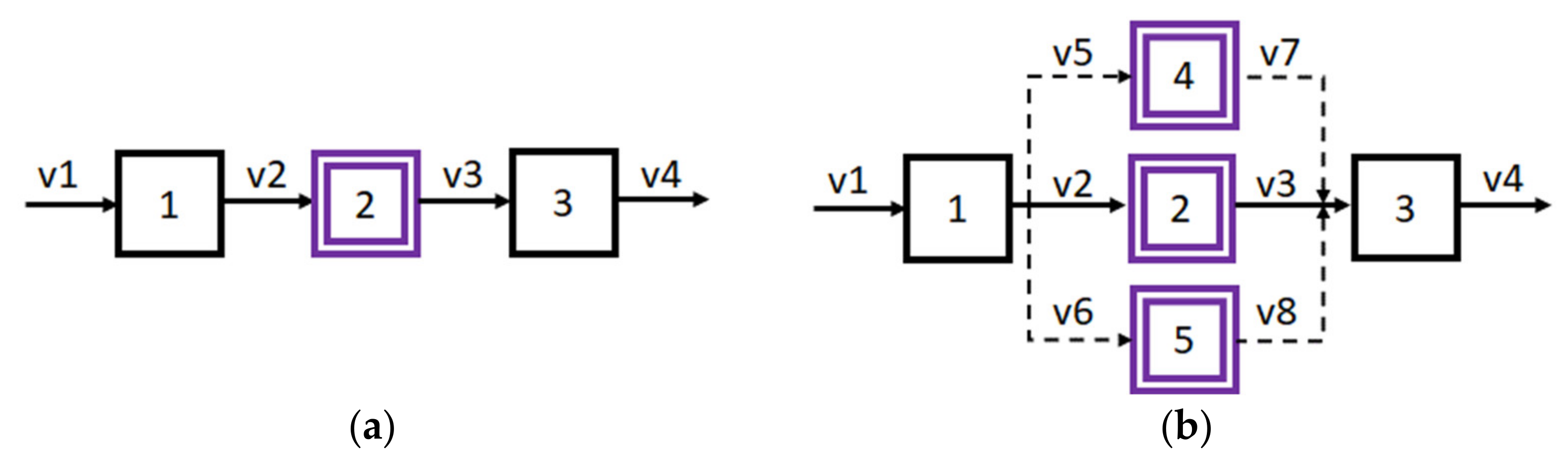
Because several models of the same device are available in the market, each of them having different sizes and technical performances, a further degree of freedom should be given to the optimizer. This means that, when looking for the optimal EH design, the combinations of all devices in terms of typology and model should be considered. Although the computational burden suffers from this implementation, it allows finding a market-oriented and thus more realistic solution. To implement both design and sizing optimization using the SMM approach, it is necessary to proceed by steps, as shown by a trivial example in Figure 1.

Initially, a general technical scheme is defined, along with connections between devices. Each device type is identified according to acronyms, and the available device models are listed on an external catalogue, where all economical and technical information are defined. Then, for each internal component, an automatic code verifies whether there are other models listed in the catalogue. Next, the EH scheme is automatically updated by substituting each original node with as many new nodes as the number of listed models. Finally, the energy vectors connecting new nodes are added. Based on the number of new nodes added in this process, the EH system is described by an upgraded general scheme with G* nodes and B* branches.

The following constraints are used to implement the optimal design and the optimal sizing dynamics within the SMM approach:

$$0\le {\mathit{A}}_{\mathit{g}}{\mathit{V}}_{\mathit{t}}\le C_g^{ max} {\delta }_g,$$

(5)

$${{\displaystyle \sum }}_{i=1}^{CT{S}_g}{\delta }_i=1.$$

(6)

Equation (5) has a twofold purpose. First, it ensures the energy vectors related to the $g$-node are bounded within zero and their maximum operational value, $C_g^{ max}$. Then, thanks to the binary decision variables ${}_g\left\{{}_1,{\dots }_{G^{*}}\right\},$ it allows whether to include devices from the upgraded general scheme. When ${\delta }_g=1$, i.e., the $g$-device is included, the related energy vectors decision variables can take any value up to $C_g^{ max}$. Instead, when ${\delta }_g=0$, i.e., the $g$-device is not included, the related energy vectors are forced to zero. As shown in Section 4.2, binary decision variables are also used to define the investment objective function. Moreover, Equation (6) ensures that only one model must eventually be selected among all those listed, being $i\left\{1,..CT{S}_g\right\}$ and $CT{S}_g$ the number of available models for the $g$-node.

2.3. Storage Constraints

The energy–time balance expressed by Equation (1) does not hold for energy storage devices (ESs). Indeed, the amounts of energy entering and leaving each ES do not necessarily coincide for a specific timestep. This is due to the possibility that ESs have to discharge part of their stored capacity. Indeed, for ESs, the left-hand side of Equation (1) is equal to the energy either withdrawn or injected into the system. To integrate ES into the problem formulation, Huang et al. [34] introduced an additional virtual node for each considered ES. Furthermore, the energy vector $v_{str,t}\in {\mathit{V}}_{\mathit{t}}$ is included to represent the charged and the discharged energy by each ES, being $str\in \left\{1,\dots ,STR\right\}$ and STR the total number of ESs in the EH. The energy balance equation for ESs becomes:

$$\left[\begin{array}{cc}\stackrel{⌣}{\mathit{Z}}& -\mathit{I}\end{array}\right]\left[\begin{array}{c}\mathit{V}\\ \Delta \mathit{E}\end{array}\right]=0.$$

(7)

Unlike electrical storage devices (EESs), the maximum capacity of thermal storage devices (TESs) is given by a volumetric water capacity. Besides, their charging and discharging phases are typically managed to maintain the internal temperature within a predefined temperature range. Although temperature-dependent operation could be implemented, handling temperature dynamics in an energy-based formulation is not practical. For this reason, all TESs in this paper are modeled following an EES approach. The equivalent kWh maximum capacity is given by:

$$s_{str}^{max}=Vo{l}_{str} cp \Delta T/3600$$

(8)

where $Vo{l}_{str}$ is the volume in liters of the $str$-TES, $cp$ is the water specific heat, and $\Delta T$ is the maximum deviation allowed between minimum and maximum internal temperature. Then, the capacity of all TESs is computed as follows:

$$s_{str,t}=s_{str,t-1}+v_{str,t}-K_{str}^{loss}\left(T_{str,t}^{op}-T^{TR}\right),$$

(9)

$$T_{str,t}^{op}=T_{str}^{min}+\frac{s_{str,t-1}}{s_{str}^{max}}\mathsf{\Delta }T,$$

(10)

$$T_{str}^{min}=T_{str}^{out}-\mathsf{\Delta }T/2.$$

(11)

Equation (9) calculates the current thermal capacity state considering the previous capacity state, the energy exchanged by the virtual node, $v_{str,t}$, along with the product of the stationary loss factor, $K_{str}^{loss}$, and the difference between the internal operating temperature, $T_{str,t}^{op}$, and the air temperature of the technical room where the TES is installed, $T^{TR}$. Furthermore, $T_{str,t}^{op}$ is defined in (10) as the sum of the minimum internal fluid temperature, $T_{str,t}^{min}$, and a fraction of $\mathsf{\Delta }T$ depending on the ratio between the previous capacity state and $s_{str}^{max}$. Moreover, $T_{str,t}^{min}$ is computed in (11) as the difference between the setting output temperature, $T_{str}^{out}$, and half of the maximum temperature deviation allowed. Finally, TES operation is limited by the following constraints:

$$0\le s_{str,t}\le {\delta }_g s_{str}^{max},$$

(12)

$${{\displaystyle \sum }}_{i=1}^{CTSstr}{\delta }_{i}Vo{l}_i\ge k_{TES}{{\displaystyle \sum }}_{u=1}^{UPstr}{\delta }_g{C}_g^{max}.$$

(13)

Equation (12) does not only limit the thermal capacity within $s_{str}^{max}$, but it also allows whether to include the $str$-device into the final system configuration. Constraint (13) ensures that the volume of the TES model chosen on the $g$-node is greater than the product of the safety factor, $k_{TES}$, and the overall capacity of the upstream thermal generators feeding the $g$-node [37,38]. Herein, $u\in \left\{1,\dots , UPstr\right\}$, while $UPstr$ and $CTSstr$ represent the number of upstream nodes and the number of available storage models of the $str$-device, respectively.

2.4. Multiple Thermal Outputs Constraints

Devices able to provide different energy services (e.g., gas boilers producing both heating and DHW) are modeled as multi input multi output components [33]. As a result, the number of input ports is equal to the number of output ports. This allows to easily recognize the input branches responsible for each energy conversion, and it also permits to specify different and unrelated energy conversions for each output carrier. Conversely, heat pumps usually give priority to DHW production over heating service in order to minimize discomfort for the users. Thus, the heat supply for space heating and DHW systems does not occur simultaneously. The following constraints are used to capture this feature:

$$0\le {\mathit{A}}_{\mathit{g}}^{\mathit{D}\mathit{H}\mathit{W}} {\mathit{V}}_{\mathit{t}}\le C_g^{max}{\mathit{M}}_{\mathit{g},\mathit{t}},$$

(14)

$$0\le {\mathit{A}}_{\mathit{g}}^{\mathit{H}} {\mathit{V}}_{\mathit{t}}\le C_g^{max}\left(1-{\mathit{M}}_{\mathit{g},\mathit{t}}\right).$$

(15)

where ${\mathit{A}}_{\mathit{g}}^{\mathit{D}\mathit{H}\mathit{W}}$ and ${\mathit{A}}_{\mathit{g}}^{\mathit{H}}$ represent the branch-port incidence matrixes for the DHW and the heating conversion, respectively. For devices capable of both heating and DHW service production, the ${\mathit{M}}_{\mathit{g},\mathit{t}}=\left\{m_{g,1},\dots ,m_{g,T}\right\}$ vector containing $T$ binary decision variables is used to set a binary control strategy. When ${\mathit{M}}_{\mathit{g},\mathit{t}}=1$, the $g$-device is enabled to produce DHW, while the heating output is forced to zero. On the other hand, when ${\mathit{M}}_{\mathit{g},\mathit{t}}=0$, the heating service is allowed, and DHW service is denied.

2.5. Solar Equipment Roof Constraints

When including PV and SCs into the EH system, additional constraints regarding the available space on the roof must be considered. Indeed, in real case application, the available surface on a roof is not just limited in space, but it is also made up of many sectors, each of them having different areas, orientations, and tilt angles. All of these parameters greatly influence the EH system sizing and operation, leading to different combinations of PV and SC surfaces according to the considered objective function.

Similar to the multi sizing procedure explained in Section 2.2, nodes representing either PV or SC are split into $R$ nodes, being $R$ the number of sectors of the roof and $r\in \left\{1,\dots ,R\right\}$. Then, branches between upstream and downstream nodes are added. Hence, the installation of PV and SC on each sector is subject to the following constraints:

$$A_r^{PV/SC}=n_r^{PV/SC} S{Z}^{PV/SC},$$

(16)

$${\delta }_r S{Z}^{PV/SC}\le A_r^{PV/SC}\le {\delta }_r S{Z}_r^R,$$

(17)

$$v_r^{PV/SC}={\eta }^{PV/SC}{A}_r^{PV/SC}{I}_r,$$

(18)

$$A_r^{PV}+A_r^{SC}\le S{Z}_r^R.$$

(19)

In Equation (16), the installed PV (SC) surface on each sector, $A_r^{PV/SC}$, is defined as a multiple of one single PV (SC) module area, $S{Z}^{PV/SC}$, using the integer variable $n_r^{PV/SC}$. Constraint (17) bounds $A_r^{PV/SC}$ between $S{Z}^{PV/SC}$ and the available surface on the $r$-sector, $S{Z}_r^R$. Moreover, the binary decision variable ${\delta }_r$ is here used to choose whether to install any PV (SC) module on the corresponding sector. The energy converted by the PV (SC) on the r-sector, $v_r^{PV/SC}$, is given by Equation (18), where the sun radiation $I_r$ is multiplied by $A_r^{PV/SC}$ and the conversion efficiency ${\eta }^{PV/SC}$. Finally, Equation (19) ensures that the sum of the installed PV and SC surfaces on each sector does not exceed $S{Z}_r^R$.

3. Energy Community Model

Energy communities employ different energy carriers to satisfy the community energy consumption. Therefore, the EH approach can be implemented within the EC framework to assess the benefits of electricity sharing for both EC users and the environment.

Initially, each final energy use must be acknowledged as a domestic or a communal load. In the first case, loads are met importing energy from the input buses, and no internal conversion device is needed, whereas in the latter case, energy entering the EC is converted by centralized conversion equipment owned by the community. To properly allocate electricity bills due to domestic and communal loads, tenants’ electricity consumption is measured using private energy meters, while electricity used for communal loads is tracked using a communal meter. Following current virtual self-consumption schemes [39], private and communal meters are connected to the public grid, whilst an internal grid allows the local RES generation to cover part of the communal loads. Moreover, when local RES generation exceeds the electricity demand of communal loads, electricity is sold to the public grid.

3.1. Electricity Mesurements

In this paper, thermal loads are supposed to be met using centralized devices owned by the community. Therefore, heating, cooling, and DHW demand are deemed as communal loads. Since devices converting electricity into thermal energy carriers are also included, electricity used for domestic and communal purposes must be separately measured. For this reason, two different electricity meters are modeled. All private energy meters are aggregated into one domestic meter (DM), allowing the estimation of the total domestic load, $E^{load}$, while a communal meter (CM) measures the amount of electricity used for thermal communal purposes, $E^{TH}$. The proposed EC connection to the electrical grid is modeled by Equations (20)–(23):

$$E_t^{SS,in}=E_t^{D,def}+E_t^{C,def},$$

(20)

$$E_t^{SS,out}=E_t^{sur},$$

(21)

$$E_t^{TH}-E_t^{PV}=E_t^{C,def}-E_t^{sur}-E_t^{sh},$$

(22)

$$E_t^{load}=E_t^{D,def}+E_t^{sh}.$$

(23)

The electricity imported from the closest substation (SS), $E_t^{SS,in}$, is defined in (20), where $E_t^{D,def}$ and $E_t^{C,def}$ stand for the electricity purchased for meeting domestic and communal demands, respectively. In (21), the electricity effectively sent to the SS, $E_t^{SS,out}$, is set equal to the surplus energy of the EC system, $E_t^{sur}$. As stated in (22), when the electricity generated by the overall PV system, $E_t^{PV}$, falls below $E_t^{TH}$, electricity is withdrawn from the SS, entering the CM. Alternatively, when $E_t^{PV}$ exceeds $E_t^{TH}$, the surplus PV generation exiting the CM can be either sent to the SS by $E_t^{sur}$ or shared to the DM via $E_t^{sh}$. Finally, in (23), $E_t^{load}$ can be matched either by importing electricity from the SS or by sharing PV generation.

3.2. Shared Electricity Pricing

Due to the virtual self-consumption regulation currently in force, energy and financial cash-flows do not coincide. Indeed, under the current regulation, shared electricity is considered as the minimum between the domestic electricity consumption and local RES generation exceeding electrical communal demand. The latter term represents the energy exiting the CM, given by the sum of surplus and shared electricity. Within this framework, electricity from the grid must be purchased at the retail price, ${\pi }^{SS,in}$, and all the electricity exceeding communal purposes is sold to the main grid at a given price, ${\pi }^{SS,out}$.

Hence, the cost-effectiveness of the shared electricity incentives can only be appreciated once the corresponding remuneration is received by the EC together with the energy bill. To integrate this postponed remuneration into an operation optimization problem, the shared electricity net value is defined as:

$${\pi }^{sh}={\pi }^{SS,in}-{\pi }^{SS,out}-{\pi }^{inc}.$$

(24)

where the retail price, ${\pi }^{SS,in}$, is reduced by both ${\pi }^{SS,out}$ and the incentive remuneration, ${\pi }^{inc}$, given for each unit of shared electricity. As a consequence, the optimal dispatch of all thermal devices strongly depends on the resulting value of ${\pi }^{sh}$, causing $E^{PV}$ to be differently allocated between $E^{TH}$, $E^{sur}$, and $E^{sh}$.

4. Problem Formulation and Methodology

4.1. EC Topologic Implementation

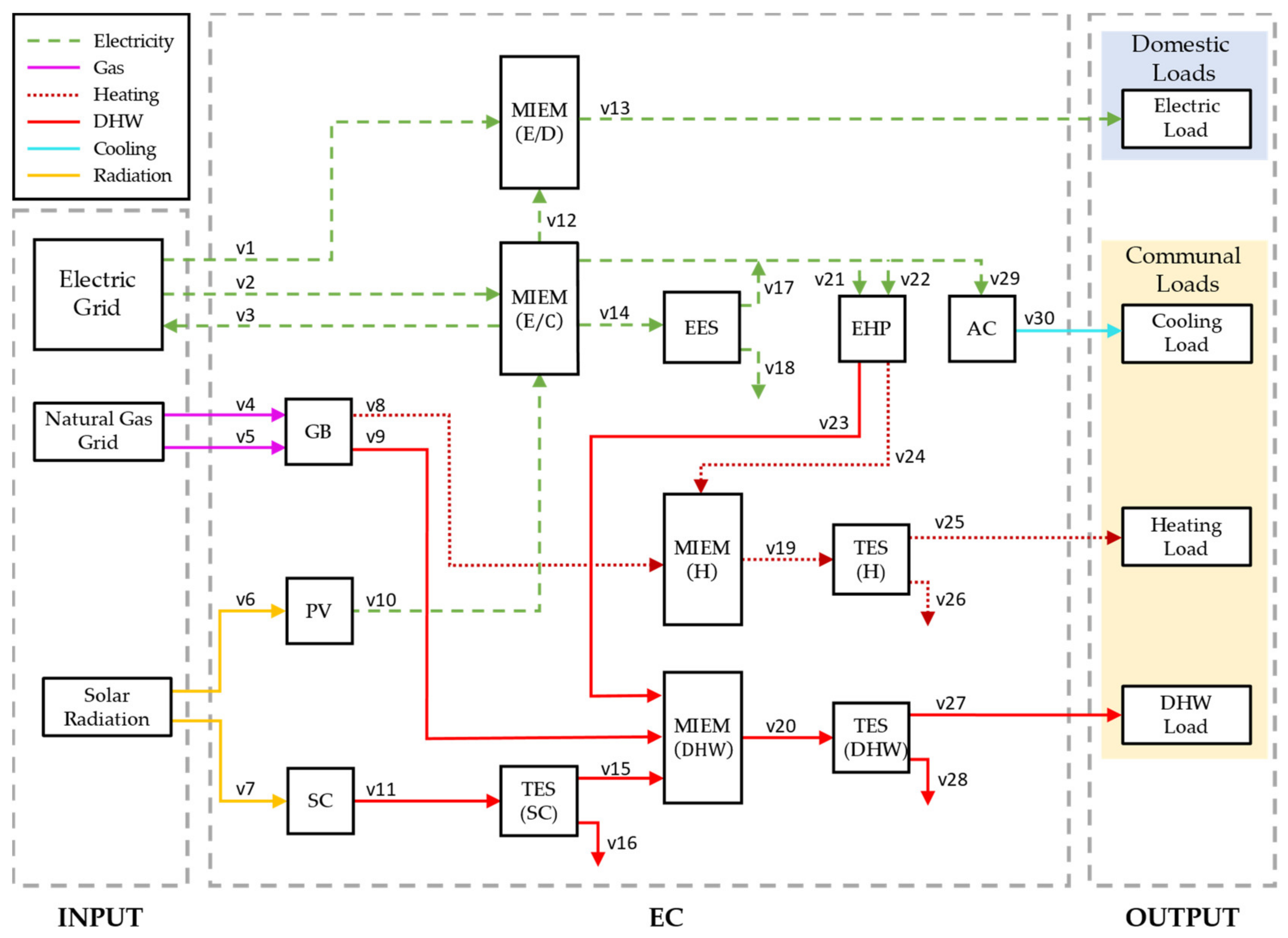
In this paper, the EC input nodes are supposed to be connected to the electrical and the natural gas distribution grids. Solar radiation is also supposed to enter the EH via a virtual input node. The output nodes are represented by electric, cooling, heating, and DHW loads, which are differentiated into domestic and communal loads, as explained in Section 3.1. The starting configuration of the EC given to the optimizer is illustrated in Figure 2.

As defined by the SMM approach, energy vectors are represented as unidirectional arrows. In this paper, four different types of internal energy carriers are considered: electricity (E), space heating (H), domestic hot water (DHW), and cooling.

In the initial configuration, the following conversion devices are included: gas boiler (GB), electrical heat pump (EHP), direct expansion multi-split systems for space cooling (AC), photovoltaic panel (PV), solar thermal collector (SC). Carriers E, H, and DHW can benefit from storage components, named EES, TES(H), and TES(DHW), respectively. To allow the dispatching of SCs, a dedicated storage unit is also included, TES(SC). Lastly, multiple interface energy management (MIEM) components are used to interface different devices with the same energy carrier, allowing to merge and split the connected energy vectors.

Once the initial configuration is determined, an automatic code skims over the catalogue of devices checking all available models. It is worth recalling that, for solar components, the optimizer does not only choose the most appropriate model in the catalogue, but it also decides the number of single solar modules to be installed on each sector of the roof.

As it can be noticed, the EC topologic implementation shown in Figure 2 satisfies Eqations (20)–(23) according to the definition of DM and CM energy meters. In

Table 1. Relationships between EC variables and energy vectors.

Variables	Energy Vectors
$E_t^{D,def}$	v1
$E_t^{C,def}$	v2
$E_t^{sur}$	v3
$G$	v4 + v5
$E_t^{PV}$	v10
$E_t^{sh}$	v12
$E_t^{TH}$	v21 + v22 + v29

, the relationships between energy vectors and variables of the EC model are listed. The gas imported, $G$, to fuel the GB for heating and DHW purposes is also included.

It should be noticed that, while $E_t^{load}$ does not offer any flexibility to the optimizer due to its predefined profile, $E_t^{TH}$ can be optimized by dispatching thermal devices according to the considered objective function.

4.2. Objective Function

To find the optimal configuration and the optimal operation of the EC considering current incentives on shared electricity, the following objective function is proposed:

$$\min CI+CO,$$

(25)

$$C{I}^D={\sum }_{g=1}^{G^{*}}{\delta }_g\left[\frac{1}{\left(r_g+1\right)}\frac{r_g{\left(r_{g+1}\right)}^{k_g}}{{\left(r_{g+1}\right)}^{k_g}-1}C{I}_g\left(1+{\sum }_{r=1}^R{n}_{g,r}^{PV/SC}\right)\right],$$

(26)

$$CO={\sum }_{d=1}^D{\lambda }_d\left( {\sum }_{t=1}^T{C}_{d,t}^{SS}+C_{d,t}^{inc}+C_{d,t}^{gas}\right),$$

(27)

$$C_{d,t}^{SS}=E_{d,t}^{SS,in}{\pi }^{SS,in}-E_{d,t}^{SS,out}{\pi }^{SS,out},$$

(28)

$$C_{d,t}^{inc}=E_{d,t}^{sh} {\pi }^{sh},$$

(29)

$$C_{d,t}^{gas}=G_{d,t} {\pi }^{gas}.$$

(30)

As stated in (25), the problem solution is given by the sum of investment and operating costs, whose terms are defined in detail in (26)–(30). The investment cost is defined in (26) as the sum of present values of yearly payments related to all devices chosen by the optimizer, i.e., those devices having ${\delta }_g=1$. Moreover, $C{I}_g$, $r_g$, and $k_g$ represent the investment cost, the interest rate, and the lifetime of the $g$-th device. The investment cost for solar devices is given by the sum of all solar units installed on each sector of the roof. Note that, in this paper, maintenance costs are also included in $C{I}_g$.

Being $d\in \left\{1,\dots ,D\right\}$ and $D$ the number of reference day in a year, Equation (27) computes the yearly operation cost as the sum of each $d$-operation cost weighted by the corresponding number of represented days, ${\lambda }_d$ (details are reported in Section 5.2). Moreover, each $d$-operating cost is defined as the sum of the following terms: (i) $C_{d,t}^{SS}$, i.e., the electricity transaction cost between the main grid and the EC (28); (ii) $C_{d,t}^{inc}$, i.e., the shared electricity cost (29); (iii) $C_{d,t}^{gas}$, i.e., the cost for purchasing gas at the retail price ${\pi }^{gas}$ (30). While ${\pi }^{SS,in}$,${\pi }^{SS,out}$, and ${\pi }^{gas}$ prices are set by energy retailers, ${\pi }^{inc}$ depends on incentives given by the particular self-consumption scheme, as previously considered in Section 3.2.

5. Case Study

5.1. Building and Climate Data

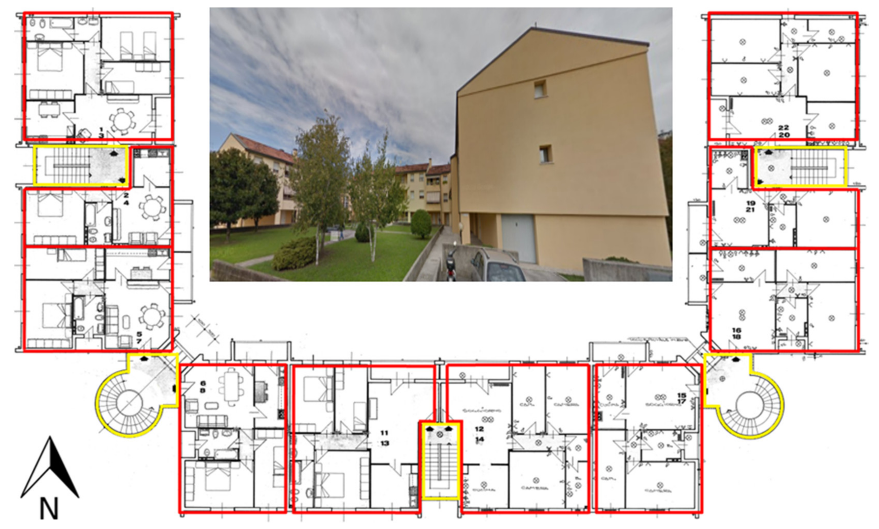
The approach for the design and the operation of the EC system is applied to a residential building containing 22 apartments located in the northeast of Italy near Treviso. The building was built in 1989 and consists of three interconnected blocks with three floors. The planimetry of the first and the second floor is shown in Figure 3, where the dwellings are contoured in red, and the unheated spaces are highlighted in yellow. The ground floor is almost entirely used as garages, except for the central part of the main block, occupied by two apartment units. The first floor is partly on a portico, and there is an unheated crawl space between the second floor and the gable roof, whose pitch is 22°.

The overall heated and cooled floor area is 1480 m^2, and the ratio between external surfaces and the conditioned volume is 0.81 m²/m³. The external walls are made of hollow bricks, and there are aluminum double-pane windows. The main thermal properties of the external opaque and the glazed components are listed in

Table 2. Properties of the main opaque components and windows.

Components	Main Properties
External walls	U-value = 0.92 W/(m2K)
Ground floor	U-value = 0.87 W/(m2K)
Other floors	U-value = 1.29 W/(m2K)
Upper-level ceiling	U-value = 1.58 W/(m2K)
Windows, glazing	U-value = 2.83 W/(m2K)	g-factor = 0.755
Windows, frame	U-value = 7.00 W/(m2K)	Aframe/Awindow = 0.15

.

The entire building is modeled considering 22 heated/cooled zones (i.e., all the apartments) and 14 unconditioned zones (five zones for the stairs, three zones for the crawl spaces, six zones for garages and technical rooms).

As regards space heating, the internal air temperature was set to 20 °C, with an overnight reduction to 18 °C from 23:00 to 07:00. During the cooling season, indoor air was set to 26 °C with a maximum 50% of relative humidity. The infiltration rate of the heated/cooled zones was set to 0.3 volumes per hour. Internal heat gains were modeled using standards and the profiles from a large monitoring campaign conducted in Italy [40,41,42]. The climate data of Treviso was considered by means of the corresponding test reference year taken by the well-known EnergyPlus weather data repository [43]. In this climatic zone, the heating period lasts 183 days, from 15 October to 15 April. The corresponding number of heating degree days is 2456.

Various solutions can be evaluated for the retrofit of the considered building to improve its energy performance as well as the tenants’ thermal comfort. The replacement of the windows and the insulation of the opaque components are initially considered separately and later combined together. As regards glazed components, new uPVC double-pane windows filled with Argon are considered with an overall U-value of 1.4 W/(${\mathrm{m}}^2\mathrm{K}$) and a g-factor of 0.589. As regards opaque components, EPS boards with thermal conductivity of 0.04 W/(m²K) and thickness of 15 cm are considered for the insulation of the external walls and the ceiling of the portico. The ceiling of the second floor is insulated from the side of the crawl space, reaching a thermal transmittance of 0.3 W/(${\mathrm{m}}^2\mathrm{K}$). The floor of the first floor is insulated from the side of the garages, considering a board with a thermal resistance of 2.55 ${\mathrm{m}}^2\mathrm{K}$/W made of 2.5 cm of cement-bonded wood fiber coupled with 8 cm of mineral wool; in terms of fire resistance, this material is suitable to be used in garages. More details about the climate data and the annual energy demand in the simulated scenarios are given in Appendix A.

5.2. Demand Evaluation and Reference Days

Based on the building technical data presented in the previous section, building simulations are performed using TRNSYS 17, a well-known software for detailed dynamic building simulations [44], with a 15 min resolution timestep. The results of the simulations allow the assessment of heating and cooling load profiles under the following refurbishment cases: (i) no intervention made; (ii) windows replacement; (iii) envelope replacement; (iv) windows and envelope replacement. The annual DHW consumption is evaluated using a statistical model proposed by Jordan et al. [45]. Finally, the electric load profile of the EC is obtained aggregating real data consumption of the considered 22 housing units.

Considering yearly-based profiles in optimization applications leads to very accurate problem solutions, although it causes extremely time-consuming simulations. For this reason, yearly-based data regarding demand consumption and external parameters (e.g., sun radiation and outdoor temperature) must be boiled down to a limited number of reference days throughout the year. Based on homogeneous characteristics of yearly demand and external signals profiles, five seasonal periods are identified, similarly to what was done in [35]: (i) very cold with low insolation; (ii) cold with medium insolation; (iii) mid-season; (iv) hot; (v) very hot. Results are shown in

Table 3. Reference days considered in the analysis.

$d$	Periods of the Year	${\lambda }_d$
1	1 December–28 February	90
2	1 March–15 April, 16 October–30 November	92
3	16 April–31 May, 16 September—15 October	76
4	1–30 June, 16 August–15 September	61
5	1 July–15 August	46

. Each $d$-reference day profile is calculated as the mean profile of all the represented days. In conclusion, yearly profiles are approximated by the profiles of a consecutive combination of $d$-days, each of them weighted by the corresponding number of represented days, ${\lambda }_d$.

To achieve representative operating results of the EC throughout the year, the operating results of each $d$-day must adequately represent the corresponding season. Because the profiles of energy demand and external parameters greatly differ one season from the other, by simulating each $d$-day consecutively, operation results are affected by inaccuracies due to time-dependent components (e.g., TESs). Indeed, charging and discharging phases of storage units greatly depend on previous and future load forecasts. Therefore, the management of storage devices is substantially distorted when demand profiles of consecutive $d$-days are too different. To avoid this type of inconsistency, each reference day is simulated five times in a row, resulting in an overall 25 days simulation. Additionally, because five identical days are considered for every season, each simulated day should be weighted by a fifth of the corresponding ${\lambda }_d$.

Since the third day of each season is the least affected by adjacent seasons, once the 25 days-based simulation is over, a post-process code extracts the operating results for every third day of each season and multiplies them by the corresponding ${\lambda }_d$. The combination of these terms is used to define the correct yearly operation result of the EC.

5.3. Technical Systems

The catalogue of devices included in this paper is listed in

Table 4. Catalogue of devices considered.

Device	Size	Life	CI	Device	Size	Life	CI
AC	35 kW	15	39,600 €	TES(H)	800 l	20	736 €
EHP	20 kW	20	7200 €		1000 l	20	779 €
	40 kW	20	14,400 €		2000 l	20	1377 €
	85 kW	20	30,600 €		4000 l	20	2713 €
	95 kW	20	34,200 €		5000 l	20	3738 €
EES	10 kWh	10	6000 €		6000 l	20	4304 €
	29 kWh	10	18,000 €		8000 l	20	5005 €
	48 kWh	10	30,000 €		10,000 l	20	6380 €
GB	24 kW	15	5767 €		16,000 l	20	10.008 €
	32 kW	15	6266 €	TES(DHW)	1000 l	20	2846 €
	44 kW	15	7133 €		1500 l	20	3814 €
	60 kW	15	8403 €		2000 l	20	5118 €
	80 kW	15	10,599 €		3000 l	20	6420 €
	105 kW	15	11,911 €		4000 l	20	8150 €
PV	1.6 m2	25	352 €		5000 l	20	9426 €
SC	2 m2	15	600 €		10,000 l	20	18.852 €
MIEM(DHW)	-	15	1 €	TES(SC)	3000 l	20	6420 €
MIEM(E)	-	15	4000 €		5000 l	20	9426 €
MIEM(H)	-	15	1000 €

AC: space cooling; EHP: electrical heat pump; EES: electrical storage devices; GB: gas boiler; PV: photovoltaic panel; SC: solar thermal collector; MIEM: multiple interface energy management; DHW: domestic hot water; TES: thermal storage devices.

. Investment costs and performances of devices currently available in the Italian market are considered to achieve market-oriented solutions.

For PV and SC components, the size value reported in Table 4 refers to the area of the PV (SC) single module, $S{Z}^{PV/SC}$. Their conversion efficiencies have nominal values equal to 0.18 and 0.8, respectively, and depend on external conditions as described in Vian et al. [33]. In this reference, PV systems depend on both outdoor temperature and sun radiation, while SCs’ performance is only affected by sun radiation. Moreover, the roof of the considered building has three available sectors: (i) 165 m² facing south; (ii) 110 m² facing east; (iii) 110 m² facing west.

All ESs have constant charging and discharging efficiencies set to 0.98 and 0.99, respectively. TESs are supposed to control the outlet water temperature within a range of $\pm 3 °\mathrm{C}$, thus having a $\mathsf{\Delta }T=6 °\mathrm{C}$. For TESs devices with sizes smaller than 2000 l, the stationary loss factor $K_{str}^{loss}=5.37 \mathrm{W}/\mathrm{K}$ is used, whereas for bigger sizes, $K_{str}^{loss}=4.38 \mathrm{W}/\mathrm{K}$ is considered. Finally, for all TESs, $k_{TES}$ = 20 l/kW is used based on common design practice.

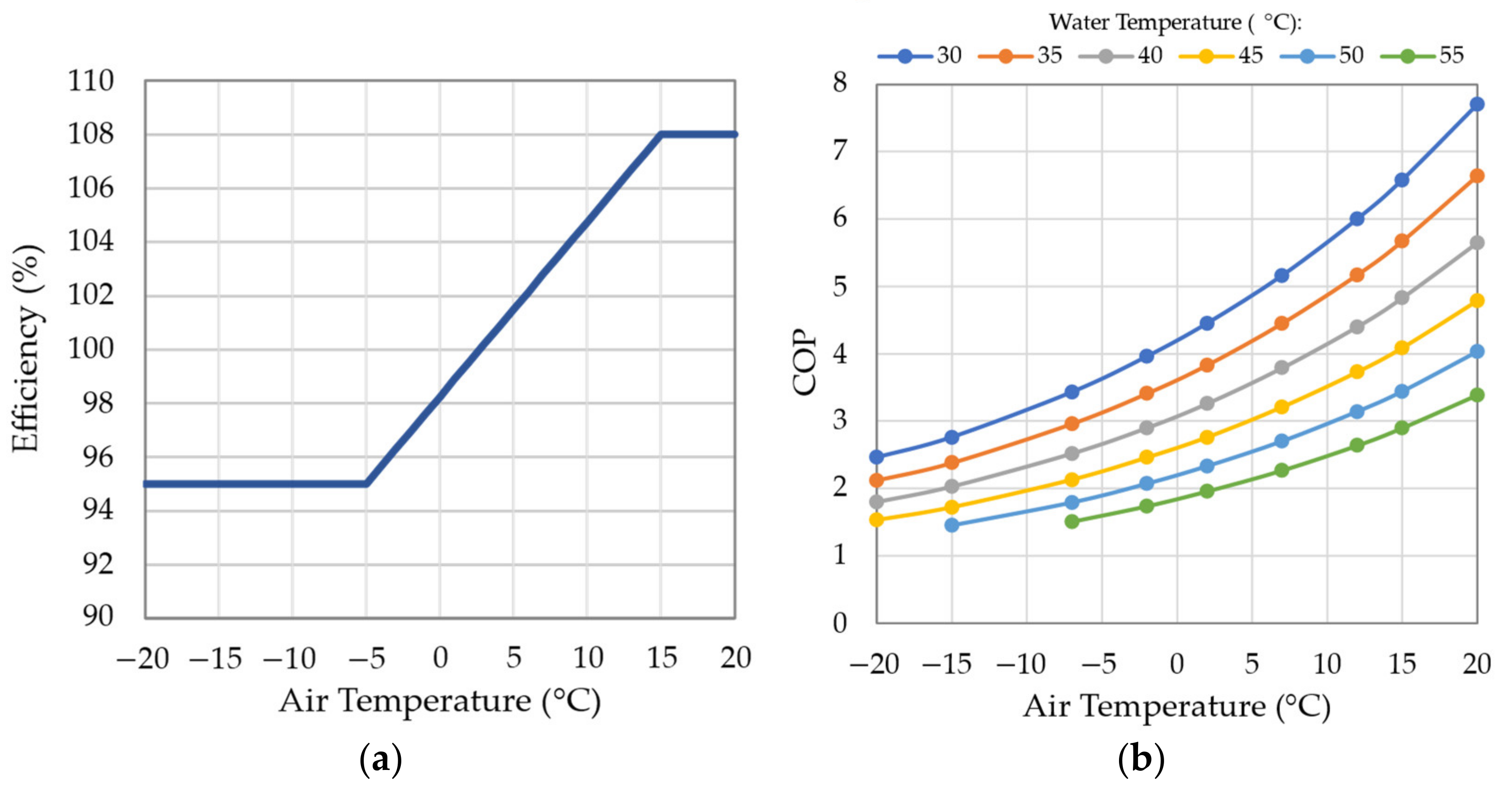
Real performances of condensing gas-fired boilers and air-to-water heat pumps are used to model the dependency on outdoor air temperature of GB and EHP. In Figure 4a, the GB implemented conversion efficiency is presented, while in Figure 4b, the coefficient of performance (COP) of the EHP is shown for different values of water temperature production.

The investment costs associated with MIEMs include all those technical expenditures needed for practical installation. As an example, the MIEM(E) cost includes all purchases for wiring and protection equipment. Moreover, the investment cost of MIEM(H) is supposed to include the installation cost related to the DHW system. Finally, the present value of yearly payments of all devices is calculated using a fixed interest rate $r=4\%$.

5.4. Investment Scenarios and Operating Assumptions

To assess the most suitable investment solution, five scenarios are investigated, and their features are reported in

Table 5. Description of considered scenarios.

Scenario	Refurbishment Intervention	Retrofit Cost	Catalogue	${\mathit{T}}^{\mathit{w}}$
S-B	No intervention	0	GB, TESs, AC	55 °C
S-H	No intervention	0	full	55 °C
S-W	Windows replacement	60,953 €	full	50 °C
S-E	Envelope replacement	125,304 €	full	50 °C
S-WE	Scenario W + Scenario E	186,257 €	full	45 °C

. They do not only differ in terms of retrofit intervention but also for the temperature of the water supplying the heating system, $T^w$, and for the typology of devices included in the initial configuration.

Scenario S-B is used as a benchmark scenario where no other devices other than GBs, AC, and MIEMs together with TES(H)s and TES(DHW)s can be chosen, and no refurbishment intervention is made. This is supposed to represent the majority of current fossil-based thermal systems with no local generation available. In addition, because PVs cannot be installed, remuneration for shared electricity cannot take place. Scenario S-H is a hybrid scenario where no intervention is considered but where the energy system is designed according to the general configuration displayed in Figure 2. Scenarios S-W, S-E, and S-WE are also configured according to the general initial configuration while benefitting from a progressive increase in building efficiency. Besides, as the building efficiency increases, radiators are supplied with lower $T^w$, hence progressively improving the performance of heating devices. In all scenarios, DHW is supplied at a temperature of 55 °C. Lastly, all retrofit intervention investment costs are supposed to be split into 25 yearly payments with a fixed interest rate $r=4\%$.

Electricity retail price ${\pi }_{in}^{SS}$ is set at $0.19€/{\mathrm{kWh}}_{\mathrm{e}}$, while surplus energy injected into the grid is remunerated at ${\pi }_{in}^{SS}=0.05€/{\mathrm{kWh}}_{\mathrm{e}}$. Following current incentives by the Italian government [39], shared electricity is remunerated at ${\pi }^{inc}=0.11€/{\mathrm{kWh}}_{\mathrm{e}}$. Ultimately, natural gas retail price is set at $0.90€/\mathrm{scm}$, which translates into ${\pi }^{gas}=0.0938€/{\mathrm{kWh}}_{\mathrm{th}}$ using the conversion factor of $9.6{\mathrm{kWh}}_{\mathrm{th}}/\mathrm{scm}$.

The proposed model is implemented in the YAMILP platform [46], which allows the problem to be built within a MATLAB interface, and solved thanks to the GUROBI solver [47], one of the most used commercial solvers for linear and quadratic programming. Simulations are conducted on a 64 bit PC with a 2.80 GHz CPU and 16 GB RAM.

6. Simulation Results

Simulation results are used to assess the most convenient investment intervention from a short-term and a long-term perspective. Then, the overall best economic scenario is analyzed to appreciate optimal operating results. In conclusion, annual emissions generated by the EC are evaluated based on the net energy imported into the system.

6.1. Optimal Results of Considered Scenarios

Optimal design and sizing results are reported in

Table 6. Typology and size of devices included in considered scenarios.

Devices		S-B	S-H		S-W		S-E		S-WE
		-	Y	N	Y	N	Y	N	Y	N
AC	$\left(\mathrm{kW}\right)$	35	35	35	35	35	35	35	35	35
EHP	$\left(\mathrm{kW}\right)$	-	40	40	40	40	40	40	40	40
GB	$\left(\mathrm{kW}\right)$	80	44	44	32	32	-	-	-	-
TES(H)	$\left(\mathrm{l}\right)$	10,000	4000	4000	8000	8000	10,000	10,000	4000	4000
TES(DHW)	$\left(\mathrm{l}\right)$	5000	3000	3000	1500	1500	5000	5000	5000	5000
PV(EST)	$\left({\mathrm{m}}^2\right)$	-	108.8	108.8	108.8	105.6	108.8	40.0	108.8	16.0
PV(WEST)	$\left({\mathrm{m}}^2\right)$	-	108.8	59.2	108.8	40.0	108.8	40.0	108.8	12.8
PV(SOUTH)	$\left({\mathrm{m}}^2\right)$	-	164.8	164.8	164.8	164.8	164.8	164.8	164.8	164.8

. To highlight the contribution given by current incentives on shared electricity, all scenarios are simulated with (Y) and without incentives (N). The same identification was also used in

Table 7. Optimal investment and operation results.

Costs	S-B	S-H		S-W		S-E		S-WE
	-	Y	N	Y	N	Y	N	Y	N
$C{I}^D$	6238	11,663	10,991	11,566	10,591	11,518	9655	11,259	8702
$C{I}^B$	0	0	0	3752	3752	7712	7712	11,464	11,464
$CO$	33,649	22,461	24,762	18,460	21,139	13,011	16,602	10,878	15,178
$C^{tot}$	39,887	34,124	35,753	33,777	35,482	32,242	33,970	33,601	35,345

.

In all considered simulations, optimal configurations do not include EES, SC, and TES(SC) devices due to their high investment costs which are not compensated by sufficient operating energy savings. Since the 35 kW AC is the only AC model listed in the calatogue, it must be included in all scenarios. As it can be observed, shared electricity remuneration only affects the sizing of the PV system, thus not influencing the choice of other devices. Because incentives on shared electricity are so attractive, when remuneration is given to the EC, the optimizer maximizes the PV surface on each available roof sector. Instead, when electricity sharing is not remunerated, PV generation is not shared among end-users. Then, the overall size of the PV system only depends on the EHP and the AC consumption needed to meet the heating and the cooling load, respectively.

For both TES(H) and TES(DHW), sizing solutions are found within a set of three available models, namely small, medium, and large. In the benchmark scenario (S-B), heating and DHW can only be produced by the GB. Hence, an 80 kW GB together with large TESs are chosen. Although the hybrid scenario (S-H) is based on the same demand profiles of S-B, by letting the solver choose among the entire device catalogue, a different solution is found. In fact, heating and DHW loads are met using a 40 kW EHP and a 40 kW GB. Given the EHP contribution, the medium size of TES(H) and the small size of TES(DHW) are selected. The slight improvement of the building efficiency in S-W results in lower heating and cooling demands. Thus, heating peak load is covered using the 40 kW EHP, a smaller 32 kW GB, and the medium TES(H). The retrofit intervention of S-E leads to a significant reduction of the heating demand, allowing the exclusion of GB, which is balanced by using large TESs. Finally, in S-WE, the further reduction of the heating demand permits to decrease the capacity of the TES(H) to its smallest size.

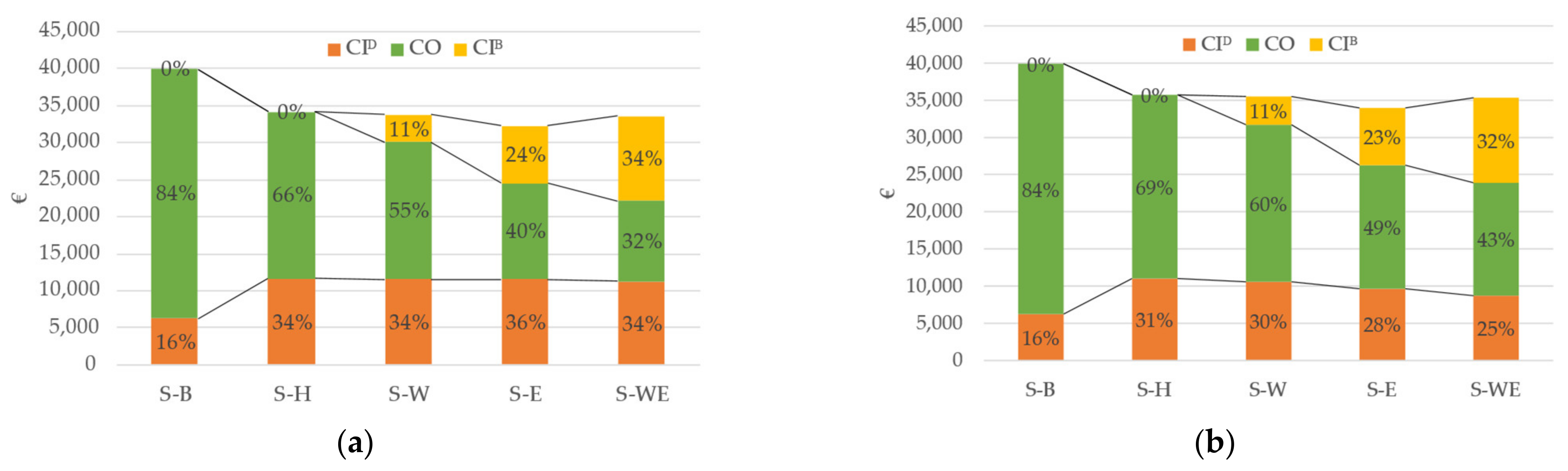
The resulting total cost is given by the sum of the operating cost ($CO$), the total investment cost for devices ($C{I}^D$), and the present value of yearly payment for retrofit intervention ($C{I}^B$). The economic results of the considered scenarios are reported in Table 7. This clearly shows that the remuneration on shared electricity leads to cheaper solutions for each considered scenario.

The values in Table 7 can be observed in Figure 5, which illustrates the results of the scenarios with (Figure 5a) and without (Figure 5b) remuneration. Although S-B shows the lowest $C{I}^D$, its operating cost is considerably higher than all other cases, thus resulting in the most expensive scenario. The $C{I}^D$ is nearly constant across all other cases, with slightly lower values when no remuneration is given due to the smaller area of the PV system installed. As might be expected, operating cost reduction can be achieved by investing in refurbishment interventions. Moreover, when shared electricity is remunerated, operating costs can be further reduced. Although S-WE guarantees the lowest operating costs, the corresponding $C{I}^B$ makes the overall solution more expensive than that of S-E. Therefore, the solution of S-E with remuneration represents the overall best.

6.2. Long-Term Economic Evaluation

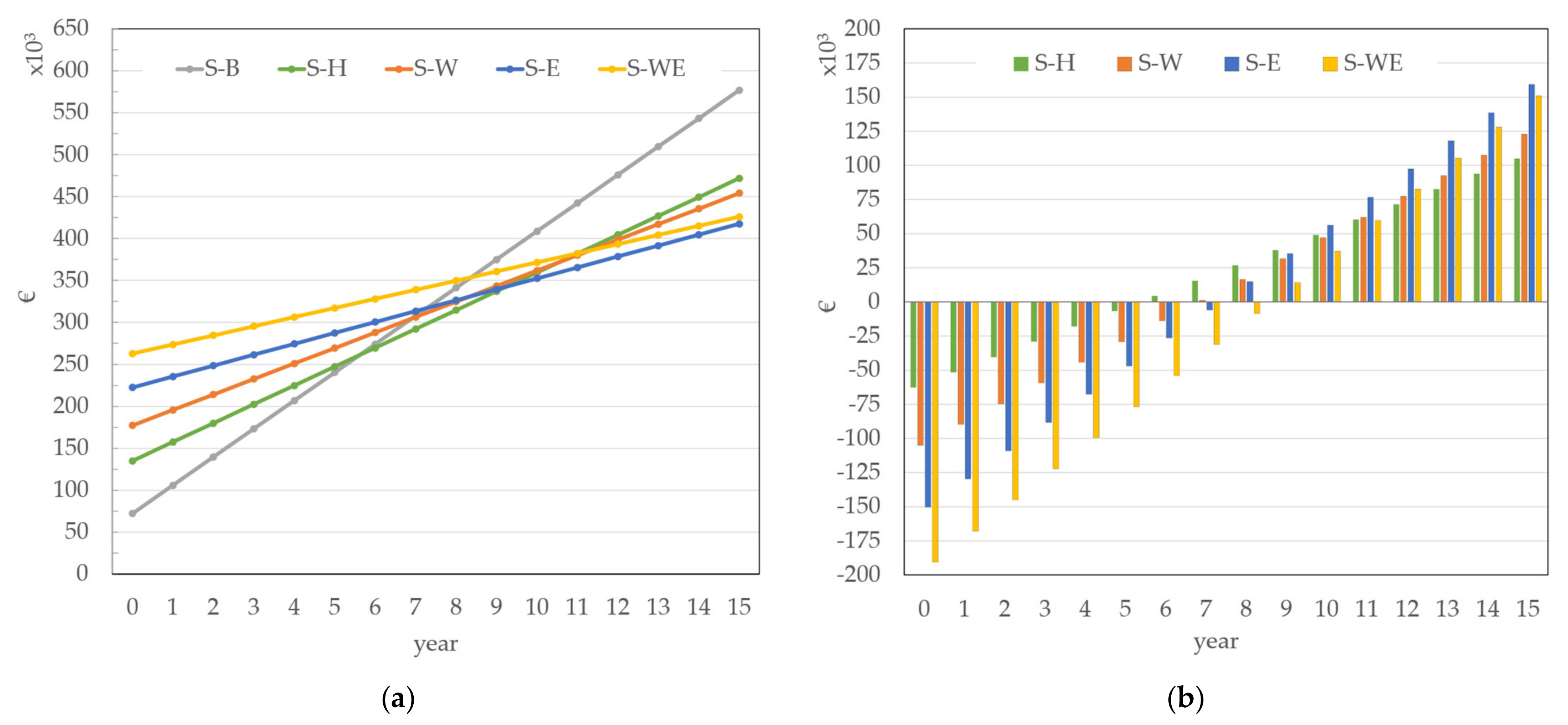
To assess the most convenient investment scenario in a long-term perspective, an economic evaluation is carried out considering only solutions with remuneration on shared electricity. The following assumptions are made: (i) 15 years time horizon, which is the shortest device lifetime among all devices included in Table 6; (ii) investments costs are distributed over the time horizon since year 0 with a fixed interest rate $r=4$%; (iii) operating costs are paid at the end of each year with no interest rate.

Because the lifetime of most devices exceeds 15 years, the present value of the whole equipment system within the considered time horizon is calculated as the sum of the first 15 yearly payments of each device, $\overline{C{I}^D}$. Similarly, retrofit interventions have 25 year payback periods; therefore, the present value of the payments made within the considered time horizon is evaluated as the sum of the first 15 yearly payments, $\overline{C{I}^B}$. The overall optimized cost of each scenario, $Cos{t}_{15}$, is computed as the sum of total investments, $\overline{C{I}^{tot}},$ and 15 times the $CO$.

The results shown in

Table 8. Present values of investment and operation results.

Scenario	$\overline{\mathit{C}{\mathit{I}}^{\mathit{D}}}$ $\left(€\right)$	$\overline{\mathit{C}{\mathit{I}}^{\mathit{B}}}$ $\left(€\right)$	$\overline{\mathit{C}{\mathit{I}}^{\mathit{t}\mathit{o}\mathit{t}}}$ $\left(€\right)$	$\mathit{C}\mathit{O}$ $\left(€/year\right)$	$\mathit{C}\mathit{o}\mathit{s}{\mathit{t}}_{\mathbf{15}}$ $\left(€\right)$
S-B	72,132	0	72,132	33,649	576,868
S-H	134,861	0	134,861	22,461	471,783
S-W	133,738	43,381	177,118	18,460	454,011
S-E	133,188	89,180	222,368	13,011	417,536
S-WE	130,188	132,561	262,749	10,878	425,917

are used to assess the progressive cost profiles of each scenario, Figure 6a, and the progressive saving profiles of each scenario compared with the benchmark scenario S-B, Figure 6b. Within the considered time horizon, S-E results in the most convenient scenario, i.e., the scenario with the overall lowest cost ($Cos{t}_{{15}_{,}\mathrm{S}-\mathrm{E}}=417,536 €$). In particular, S-E allows 159,331 € cost savings compared to S-B after 15 years. It is worth noticing that, by not choosing S-B, savings can be achieved within a time span directly related to the investment costs. The additional investment in S-H compared with S-B would be matched in 5 years, while for S-WE, it would be matched in 9 years.

6.3. Operation Analysis of the Best Scenario

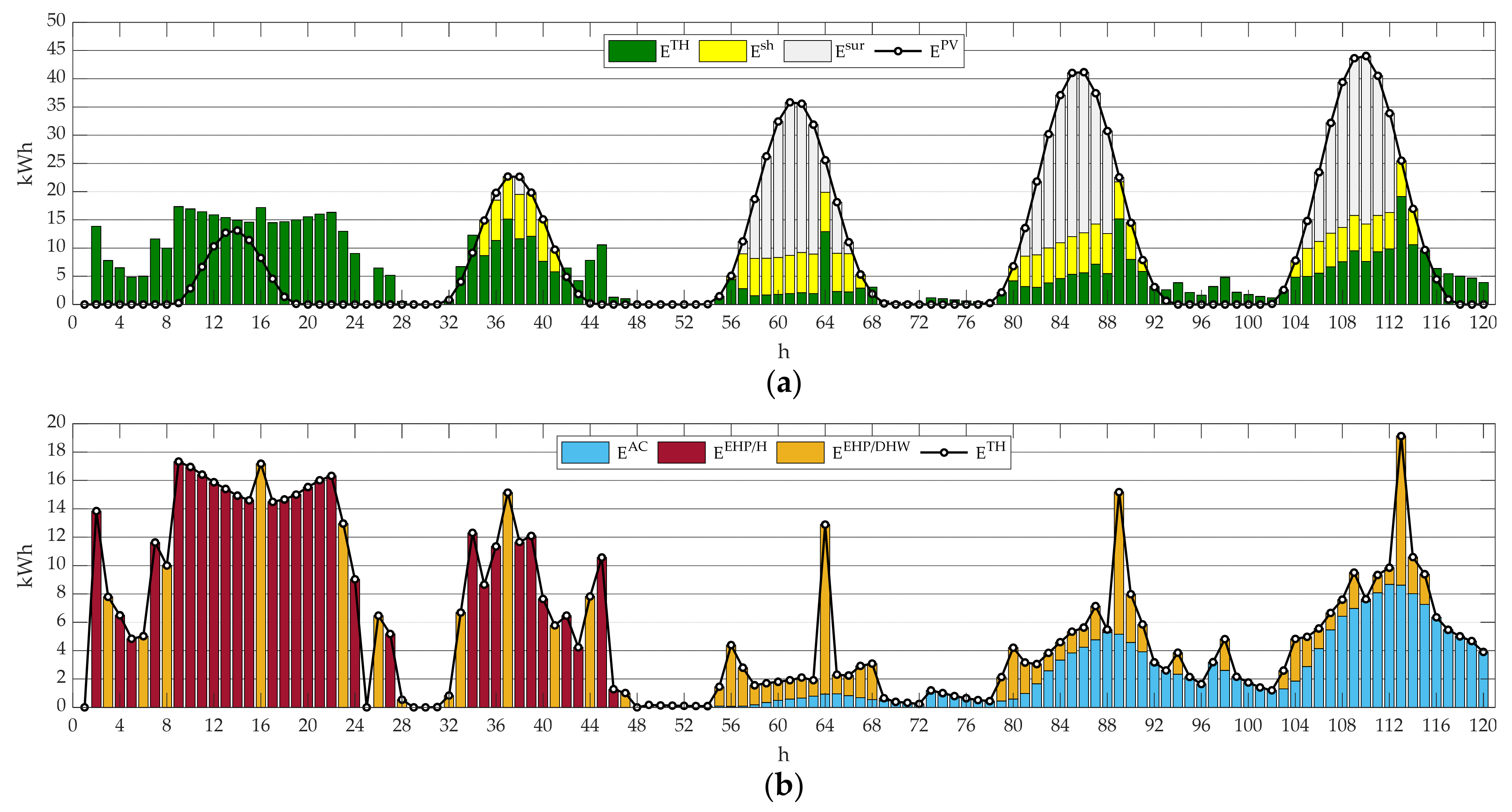
This section presents the results about the optimal operation of the economically best investment scenario, S-E. As shown in Figure 7a, PV generation cannot be shared on the first reference day, which represents very cold days with low solar radiation. This is due to high EHP consumption for space heating, as can be seen in Figure 7b. In all other reference days, PV generation exceeds $E^{TH}$, hence allowing to share electricity and eventually sell the surplus to the main grid. It is worth noticing that, thanks to the considered pricing scheme, $E^{PV}$ is distributed according to the following convenience order: $E^{TH}$, $E^{sh}$, $E^{sur}$. The optimizer recognizes that supplying shared electricity to the domestic load is more convenient than buying electricity from the distribution network at the retail price. Furthermore, this strongly encourages the optimizer to maximize the PV area on the roof, in accordance with the results in Table 6.

From Figure 7b, the composition of $E^{TH}$ can be appreciated. Although, in this paper, the management of the cooling load does not offer any flexibility, the $E^{TH}$ profile is optimized by optimally scheduling the power demand of the EHP. During cold days, the EHP is mostly used for the heating service, while DHW production occurs intermittently during the day. On milder days, the EHP operates exclusively for the DHW service, with a moderate consumption during most of the day and a significant consumption peak during sunny hours. While working at its maximum capacity from 09:00 to 22:00, the EHP consumption decreases in the central hours of the day due to the outdoor temperature rise, increasing its COP. At 16:00, the EHP consumption deviates due to the lower COP of the DHW system, which distributes DHW at a higher temperature compared to the heating system.

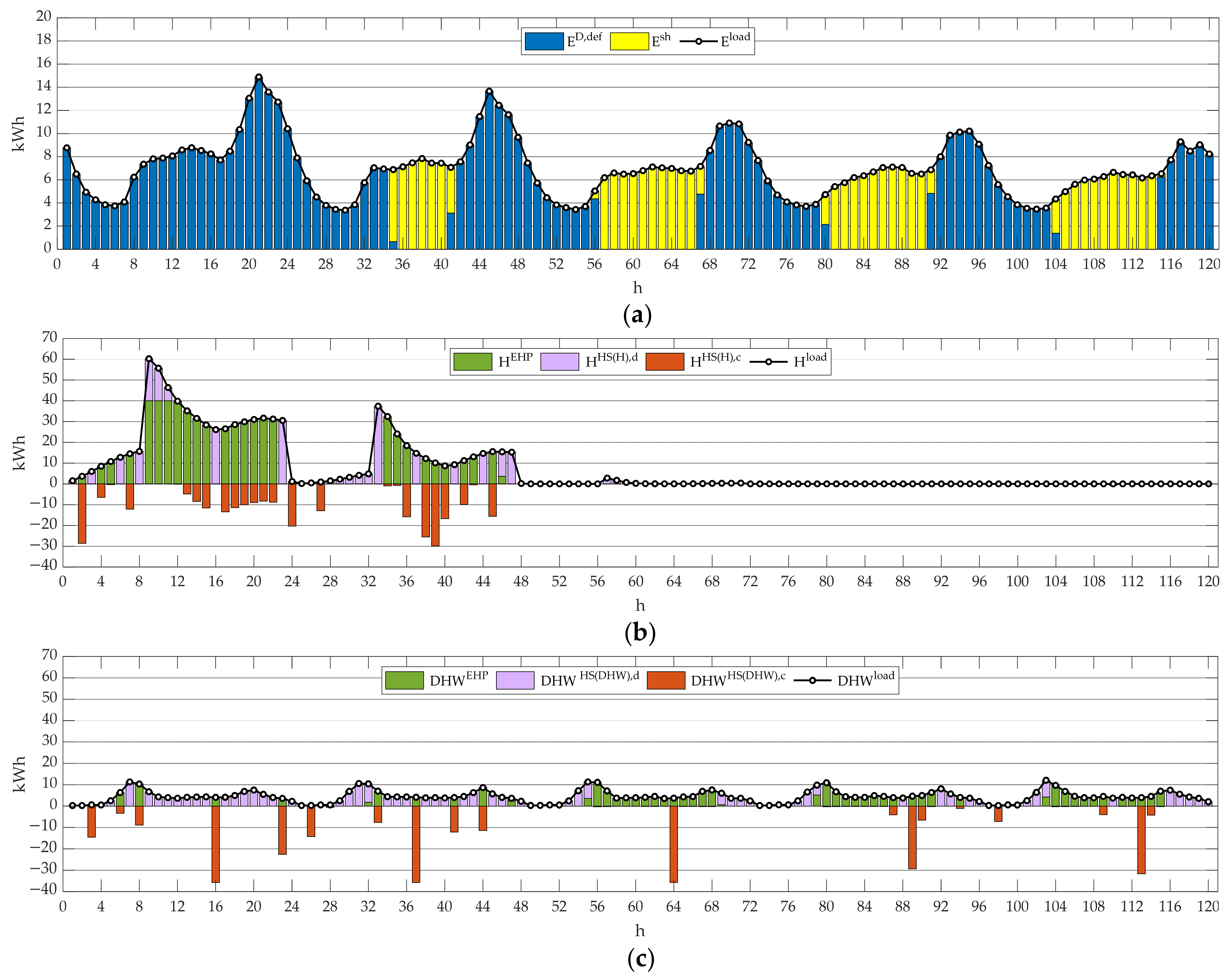
The electrical and the thermal end-use profiles are illustrated in Figure 8. In Figure 8a, the electrical load is supplied by the electricity coming from the grid and the PV-shared electricity. The supply of both heating and DHW load is secured by the EHP thermal output and by the thermal energy provided by TESs. When the EHP generation exceeds the demand, the surplus energy is used to charge the TESs. On the other hand, when the EHP generation falls below the demand, TESs discharge, matching thermal loads. During cold periods, the heating load in Figure 8b is met using mostly EHP generation while also taking advantage of the TES(H) discharge to cover its peak consumption. During these days, TES(DHW) in Figure 8c is dispatched to cover most of the DHW demand thanks to its discharged contribution while charging occasionally during the day. In warmer days, the DHW load is generally satisfied by EHP generation during sunny hours and by discharging the TES(DHW) during night-time.

6.4. Environmental Evaluation

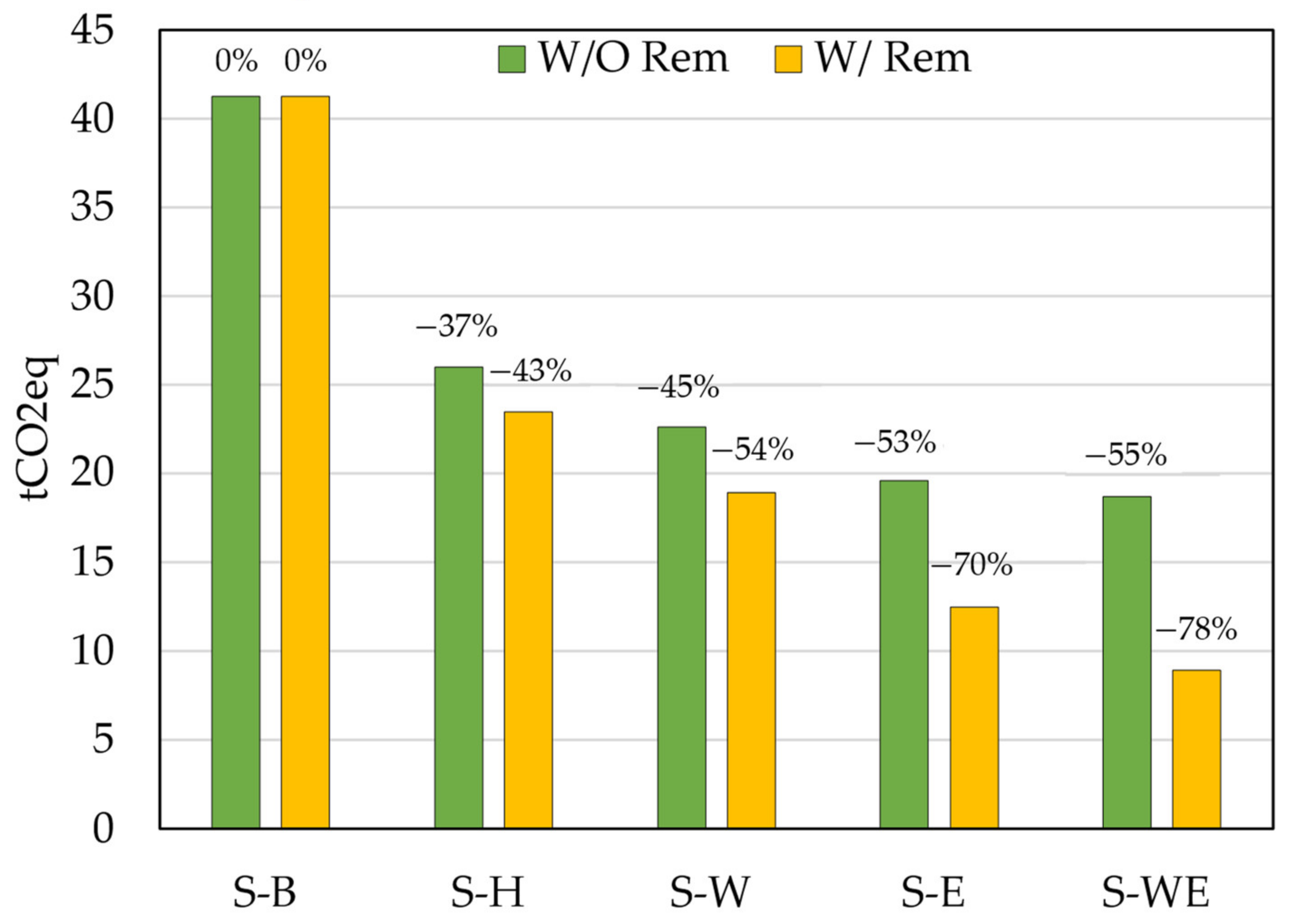
Lastly, simulation results are used to assess the environmental benefit of the considered EC and the influence of the electricity sharing incentive. Annual tons of CO₂ equivalent emissions (${\mathrm{tCO}}_2\mathrm{eq}$) are associated with the amount of net energy imported from the electrical and the gas distribution networks. For the electricity case, the net amount of imported energy is given by the difference between purchased and sold electricity. The conversion from energy to ${\mathrm{CO}}_2\mathrm{eq}$ is calculated based on: (i) emission index of Italian national generation used for electric loads ${\gamma }^e=281.4{\mathrm{gCO}}_2\mathrm{eq}/{\mathrm{kWh}}_{\mathrm{e}}$; (ii) natural gas emission index ${\gamma }^{th,gas}=201.0{\mathrm{gCO}}_2\mathrm{eq}/{\mathrm{kWh}}_{\mathrm{th}}$. As it can be seen from

Table 9. Net imported energy and corresponding CO₂eq emissions.

Scenario	Electrical Energy$\left(kW{h}_e\right)$	Thermal Energy$\left(kW{h}_{th}\right)$	Electrical Emissions ($tC{O}_{2}e{q}_e)$	Thermal Emissions ($tC{O}_{2}e{q}_{th})$	Total Emissions$\left(tC{O}_{2}e{q}_{tot}\right)$
S-B	70,398	106,702	19.81	21.44	41.25
S-H	56,715	37,265	15.96	7.49	23.45
S-W	56,278	15,269	15.84	3.07	18.91
S-E	44,312	0	12.47	0	12.47
S-WE	31,710	0	8.92	0	8.92

, emissions fall steadily with the increase of building efficiency. As might be expected, S-WE is the overall best environmental scenario, allowing a 78% emission reduction compared to S-B.

The same procedure is repeated when no remuneration is given, and the results can be observed in Figure 9.

7. Discussion

Simulation results confirm that investing in higher refurbishment interventions leads to progressively lower operating costs. Because equipment renovation costs remain approximately constant through all scenarios, the overall best economic solution can be identified based on the operating cost reduction achieved by the corresponding refurbishment investment. In this regard, the benchmark scenario S-B features the most expensive $CO$, thus resulting in it being the least convenient solution in a long-term perspective. Although the hybrid scenario S-H requires almost twice the investment of S-B, the corresponding lower $CO$ leads to an 18% reduction of $Cos{t}_{15}$. Results also prove that investing in windows replacement offers low margins for $CO$ reduction. This makes windows and envelope intervention in S-WE slightly less convenient than S-E, hence proving the envelope-only intervention to be the most convenient investment. In detail, S-WE and S-E allow 26% and 28% reduction of $Cos{t}_{15}$ compared to S-B, respectively.

Shared electricity policies have a great impact on the optimal sizing of the EC, helping to reduce the overall cost of all investment scenarios. Indeed, remuneration incentives promote further investments in PV installation, thus pushing toward higher rates of domestic electric consumption to be locally supplied. In addition, shared electricity remuneration greatly influences the environmental impact of the EC. As can be seen from Figure 9, when shared electricity is not remunerated, emissions fall at a significantly lower rate. This is mainly due to the inferior penetration of PV generation compared to solutions with remuneration. As an example, while in the case of S-WE with remuneration 382.4 m² of PV are installed, S-WE without remuneration can only benefit from 193.6 m² of PV. Therefore, shared electricity policies prove to have a twofold purpose—overall investment cost reduction and CO₂eq emissions curtailment.

8. Conclusions

In this paper, an optimal planning and operation strategy is proposed to evaluate investments for ECs under current shared electricity policies. The SMM approach is employed to model a general EC as a multi-energy EH with electric, space heating, DHW, and cooling demands. According to different refurbishment interventions, the thermal energy needs of a real multi-family building are estimated using TRNSYS software. Five investment scenarios ware evaluated based on different refurbishment interventions and different real market-available devices to be installed.

Results demonstrate that investing in building thermal efficiency leads to lower operating costs. Moreover, by reducing the building thermal needs, progressive electrification of thermal loads becomes more economically viable. This encourages end-users to take advantage of both EHP performances and local PV generation. However, as the paper demonstrates, higher intervention on building efficiency does not necessarily guarantee the overall most convenient investment, as some retrofit investments may not be compensated by corresponding operating cost reduction. For the considered case study, envelope substitution proves to be more convenient than windows replacement, allowing 28% cost reduction compared to the benchmark scenario S-B in a long-term perspective. Besides, although the combined intervention on both envelope and windows allows the lowest operating cost, the associated overall cost is higher than investing in the envelope-only substitution in both short and long-term perspectives. In conclusion, results also demonstrate that policies on shared electricity remuneration strongly encourage investments in demand electrification and local renewable installation (PV). This allows higher RES penetration into the system and further reduces both overall costs and CO₂eq emissions.

References

- Abergel, T.; Dean, B.; Dulac, J.; Hamilton, I. 2018 Global Status Report—Towards a Zero-Emission, Efficient and Resilient Buildings and Construction Sector; International Energy Agency (IEA): Paris, France, 2018; ISBN 978-92-807-3729-5. [Google Scholar]
- Kavvadias, K.; Jiménez-Navarro, J.P.; Thomassen, G.; Europäische Kommission. Gemeinsame Forschungsstelle Decarbonising the EU Heating Sector Integration of the Power and Heating Sector. 2019. Available online: https://ec.europa.eu/jrc/en/publication/decarbonising-eu-heating-sector-integration-power-and-heating-sector (accessed on 7 January 2021).
- Savaresi, A. The Paris Agreement: A New Beginning? J. Energy Nat. Resour. Law 2016, 34, 16–26. [Google Scholar] [CrossRef] [Green Version]
- Directive (EU) 2018/844 of the European Parliament and of the Council of Amending Directive 2010/31/EU on the Energy Performance of Buildings and Directive 2012/27/EU on Energy Efficiency (Text with EEA Relevance). 30 May 2018.
- Barton, J.; Huang, S.; Infield, D.; Leach, M.; Ogunkunle, D.; Torriti, J.; Thomson, M. The Evolution of Electricity Demand and the Role for Demand Side Participation, in Buildings and Transport. Spec. Sect. Transit. Pathw. Low Carbon Econ. 2013, 52, 85–102. [Google Scholar] [CrossRef] [Green Version]
- Pierro, M.; Perez, R.; Perez, M.; Moser, D.; Cornaro, C. Italian Protocol for Massive Solar Integration: Imbalance Mitigation Strategies. Renew. Energy 2020, 153, 725–739. [Google Scholar] [CrossRef]
- Jensen, S.Ø.; Marszal-Pomianowska, A.; Lollini, R.; Pasut, W.; Knotzer, A.; Engelmann, P.; Stafford, A.; Reynders, G. IEA EBC Annex 67 Energy Flexible Buildings. Energy Build. 2017, 155, 25–34. [Google Scholar] [CrossRef] [Green Version]
- Le Dréau, J.; Heiselberg, P. Energy Flexibility of Residential Buildings Using Short Term Heat Storage in the Thermal Mass. Energy 2016, 111, 991–1002. [Google Scholar] [CrossRef]
- Vivian, J.; Chiodarelli, U.; Emmi, G.; Zarrella, A. A Sensitivity Analysis on the Heating and Cooling Energy Flexibility of Residential Buildings. Sustain. Cities Soc. 2020, 52, 101815. [Google Scholar] [CrossRef]
- Directive, E.U. 2001 of the European Parliament and of the Council on the Promotion of the Use of Energy from Renewable Sources. Off. J. Eur. Union 2018, 2018, 209. [Google Scholar]
- Moroni, S.; Alberti, V.; Antoniucci, V.; Bisello, A. Energy Communities in the Transition to a Low-Carbon Future: A Taxonomical Approach and Some Policy Dilemmas. J. Env. Manag. 2019, 236, 45–53. [Google Scholar] [CrossRef]
- Caramizaru, A.; Uihlein, A. Energy Communities: An Overview of Energy and Social Innovation; Publications Office of the European Union: Bruxelles, Belgium, 2020; ISBN 92-76-10713-4. [Google Scholar]
- Roberts, J.; Frieden, D.; d’Herbemont, S.; Energy Community Definitions. Deliverable Developed Under the Scope of the COMPILE Project: Integrating Community Power in Energy Islands (Report of the European Project H2020-824424). 2019. Available online: https://www.compile-project.eu/wp-content/uploads/Explanatory-note-on-energy-community-definitions.pdf (accessed on 14 January 2021).
- Fina, B.; Auer, H.; Friedl, W. Profitability of PV Sharing in Energy Communities: Use Cases for Different Settlement Patterns. Energy 2019, 189, 116148. [Google Scholar] [CrossRef]
- Borge-Diez, D. Energy Services Fundamentals and Financing; Elsevier: Amsterdam, The Netherlands, 2020; ISBN 978-0-12-820592-1. [Google Scholar]
- Geidl, M.; Koeppel, G.; Favre-Perrod, P.; Klockl, B.; Andersson, G.; Frohlich, K. Energy Hubs for the Future. IEEE Power Energy Mag. 2007, 5, 24–30. [Google Scholar] [CrossRef]
- Frangopoulos, C.A. Optimal Synthesis and Operation of Thermal Systems by the Thermoeconomic Functional Approach. J. Eng. Gas. Turbines Power 1992, 114, 707–714. [Google Scholar] [CrossRef]
- Lazzaretto, A.; Manente, G.; Toffolo, A. SYNTHSEP: A General Methodology for the Synthesis of Energy System Configurations beyond Superstructures. Energy 2018, 147, 924–949. [Google Scholar] [CrossRef]
- Fiaschi, D.; Manfrida, G.; Petela, K.; Talluri, L. Thermo-Electric Energy Storage with Solar Heat Integration: Exergy and Exergo-Economic Analysis. Energies 2019, 12, 648. [Google Scholar] [CrossRef] [Green Version]
- Mancarella, P. MES (Multi-Energy Systems): An Overview of Concepts and Evaluation Models. Energy 2014, 65, 1–17. [Google Scholar] [CrossRef]
- Ma, T.; Wu, J.; Hao, L. Energy Flow Modeling and Optimal Operation Analysis of the Micro Energy Grid Based on Energy Hub. Energy Convers. Manag. 2017, 133, 292–306. [Google Scholar] [CrossRef]
- Urbanucci, L.; D’Ettorre, F.; Testi, D. A Comprehensive Methodology for the Integrated Optimal Sizing and Operation of Cogeneration Systems with Thermal Energy Storage. Energies 2019, 12, 875. [Google Scholar] [CrossRef] [Green Version]
- Maroufmashat, A.; Khavas, S.S.; Bakhteeyar, H. Design and Operation of A Multicarrier Energy System Based On Multi Objective Optimization Approach. Int. J. Environ. Ecol. Geol. Mar. Eng. 2014, 8. [Google Scholar] [CrossRef]
- Tzortzis, G.J.; Frangopoulos, C.A. Dynamic Optimization of Synthesis, Design and Operation of Marine Energy Systems. Proc. Inst. Mech. Eng. Part. M J. Eng. Marit. Environ. 2019, 233, 454–473. [Google Scholar] [CrossRef]
- Martinez Cesena, E.A.; Mancarella, P. Energy Systems Integration in Smart Districts: Robust Optimisation of Multi-Energy Flows in Integrated Electricity, Heat and Gas Networks. IEEE Trans. Smart Grid 2019, 10, 1122–1131. [Google Scholar] [CrossRef]
- Morvaj, B.; Evins, R.; Carmeliet, J. Optimising Urban Energy Systems: Simultaneous System Sizing, Operation and District Heating Network Layout. Energy 2016, 116, 619–636. [Google Scholar] [CrossRef]
- Qi, F.; Wen, F.; Liu, X.; Salam, A. A Residential Energy Hub Model with a Concentrating Solar Power Plant and Electric Vehicles. Energies 2017, 10, 1159. [Google Scholar] [CrossRef] [Green Version]
- Rech, S.; Casarin, S.; Silva, C.S.; Lazzaretto, A. University Campus and Surrounding Residential Complexes as Energy-Hub: A MILP Optimization Approach for a Smart Exchange of Solar Energy. Energies 2020, 13, 2919. [Google Scholar] [CrossRef]
- Wu, R.; Mavromatidis, G.; Orehounig, K.; Carmeliet, J. Multiobjective Optimisation of Energy Systems and Building Envelope Retrofit in a Residential Community. Appl. Energy 2017, 190, 634–649. [Google Scholar] [CrossRef]
- Ghorab, M. Energy Hubs Optimization for Smart Energy Network System to Minimize Economic and Environmental Impact at Canadian Community. Appl. Therm. Eng. 2019, 151, 214–230. [Google Scholar] [CrossRef]
- Manservigi, L.; Cattozzo, M.; Spina, P.R.; Venturini, M.; Bahlawan, H. Optimal Management of the Energy Flows of Interconnected Residential Users. Energies 2020, 13, 1507. [Google Scholar] [CrossRef] [Green Version]
- Huang, P.; Lovati, M.; Zhang, X.; Bales, C.; Hallbeck, S.; Becker, A.; Bergqvist, H.; Hedberg, J.; Maturi, L. Transforming a Residential Building Cluster into Electricity Prosumers in Sweden: Optimal Design of a Coupled PV-Heat Pump-Thermal Storage-Electric Vehicle System. Appl. Energy 2019, 255, 113864. [Google Scholar] [CrossRef]
- Vian, A.; Bignucolo, F.; Cagnano, A. Effects of Environmental Conditions on the Optimal Sizing and Operation of an Energy Hub. In Proceedings of the 2020 IEEE International Conference on Environment and Electrical Engineering and 2020 IEEE Industrial and Commercial Power Systems Europe (EEEIC/I&CPS Europe), Madrid, Spain, 9–12 June 2020; pp. 1–6. [Google Scholar]
- Huang, W.; Zhang, N.; Wang, Y.; Capuder, T.; Kuzle, I.; Kang, C. Matrix Modeling of Energy Hub with Variable Energy Efficiencies. Int. J. Electr. Power Energy Syst. 2020, 119, 105876. [Google Scholar] [CrossRef] [Green Version]
- Wang, Y.; Zhang, N.; Zhuo, Z.; Kang, C.; Kirschen, D. Mixed-Integer Linear Programming-Based Optimal Configuration Planning for Energy Hub: Starting from Scratch. Appl. Energy 2018, 210, 1141–1150. [Google Scholar] [CrossRef]
- Wang, Y.; Zhang, N.; Kang, C.; Kirschen, D.S.; Yang, J.; Xia, Q. Standardized Matrix Modeling of Multiple Energy Systems. IEEE Trans. Smart Grid 2019, 10, 257–270. [Google Scholar] [CrossRef]
- European Committee for Standardization EN 15450: 2007 Heating Systems in Buildings—Design of Heat Pump Heating Systems.
- European Committee for Standardization EN 14511-2:2013 Air Conditioners, Liquid Chilling Packages and Heat Pumps with Electrically Driven Compressors for Space Heating and Cooling; Test Conditions.
- Ricerca Sistema Energetico (RSE) Gli schemi di Autoconsumo Collettivo e le Comunità dell’Energia. 2020.
- Sibilio, S.; D’Agostino, A.; Fatigati, M.; Citterio, M. Valutazione Dei Consumi Nell’edilizia Esistente e Benchmark Mediante Codici Semplificati: Analisi Di Edifici Residenziali. Report ricerca di sistema elettrico. ENEA. 2009. [Google Scholar]
- Progetti-MICENE-EERG. Available online: http://www.eerg.it/index.php?p=Progetti_-_MICENE (accessed on 5 January 2021).
- Sidler, O. Project EURECO Demand Side Management—End–Use Metering Campaign in 400 Households of the European Community—Assessment of the Potential Electricity Savings—SAVE Programme; ENERTECH: Félines/Rimandoule, France, 2002. [Google Scholar]
- U.S Department of Energy (DOE). Energy Efficiency and Renewable Energy, EnergyPlus Weather Data 2003. Available online: https://energyplus.net/weather (accessed on 20 January 2021).
- Solar Energy Laboratory. TRNSYS 17 Reference Manual; University of Wisconsin-Madison: Madison, WI, USA, 2012. [Google Scholar]
- Jordan, U.; Vajen, K.; Kassel, U. DHWcalc: Program To Generate Domestic Hot Water Profiles With Statistical Means For User Defined Conditions. In Proceedings of the 2005 ISES Solar World Congress, Orlando, FL, USA, 8–12 August 2005. [Google Scholar]
- Lofberg, J. YALMIP: A Toolbox for Modeling and Optimization in MATLAB. In Proceedings of the 2004 IEEE International Conference on Robotics and Automation (IEEE Cat. No. 04CH37508), Taipei, Taiwan, 2–4 September 2004; pp. 284–289. [Google Scholar]
- Gurobi—The Fastest Solver. Available online: https://www.gurobi.com/ (accessed on 4 January 2021).
Figure 1.
Multi-sizing implementation: (a) initial layout; (b) upgraded layout.
Figure 2.
Initial topologic layout of the considered energy community (EC).
Figure 3.
Building street view and floor plan of the first and the second floor.
Figure 4.
Outdoor temperature dependency of thermal devices: (a) condensing gas-fired boiler efficiency; (b) coefficient of performance of an air-to-water electric heat pump.
Figure 5.
Optimal investments and operation results: (a) with incentives; (b) without incentives.
Figure 6.
The 15 year projection economic analysis of: (a) cumulative costs; (b) cumulative savings compared to S-B.
Figure 7.
Simulation results: (a) distribution of PV generation among the supply of communal loads, shared, and surplus electricity; (b) dispatch of thermal communal units.
Figure 8.
Energy end-use profiles: (a) electrical load; (b) heating load; (c) DHW load.
Figure 9.
Tons of CO2eq emissions for scenarios without and with incentives on shared electricity. Percentage values indicate the emission percentage reductions compared with S-B.