A Residential Energy Hub Model with a Concentrating Solar Power Plant and Electric Vehicles

Abstract

Renewable energy generation and electric vehicles (EVs) have attracted much attention in the past decade due to increasingly serious environmental problems as well as less and less fossil energy reserves. Moreover, the forms of energy utilization are changing with the development of information technology and energy technology. The term “energy hub” has been introduced to represent an entity with the capability of energy production, conversion and storage. A residential quarter energy-hub-optimization model including a concentrating solar power (CSP) unit is proposed in this work, with solar energy and electricity as its inputs to supply thermal and electrical demands, and the operating objective is to minimize the involved operation costs. The optimization model is a mixed integer linear programming (MILP) problem. Demand side management (DSM) is next implemented by modeling shiftable electrical loads such as EVs and washers, as well as flexible thermal loads such as hot water. Finally, the developed optimization model is solved with the commercial CPLEX solver based on the YALMIP/MATLAB toolbox, and sample examples are provided for demonstrating the features of the proposed method.

1. Introduction

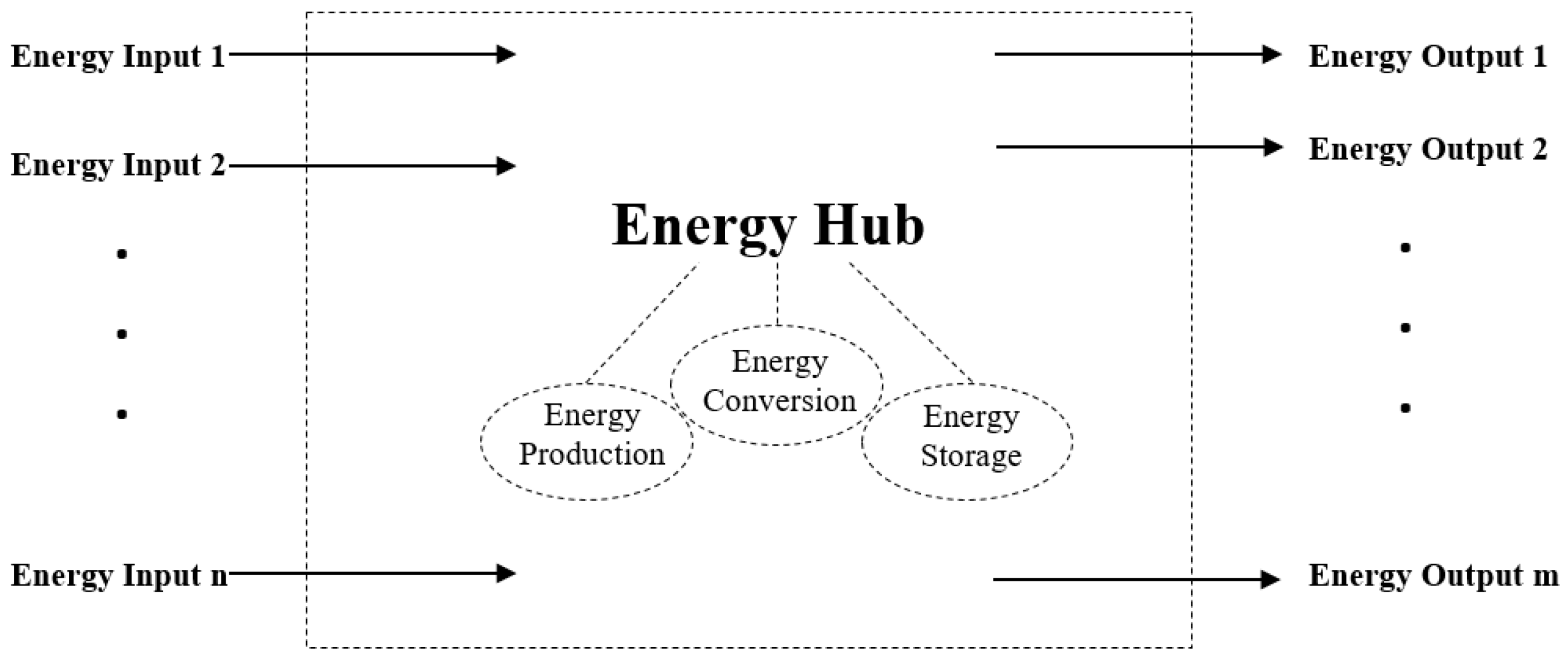
The technical basis and organizational structure of the energy industry are gradually changing due to less and less reserves of fossil fuels and increasingly serious environmental problems [1,2,3]. More efficient, sustainable and safer utilization modes of energy are gaining much attention. The conception of the “energy internet” was first proposed in [4]. A new energy utilization system, which is a combination of new energy technologies and information technology, was introduced and named “energy internet”. As one of the important parts of the energy internet, the term “energy hub” was first proposed in [5], and defined as a virtual entity consisting of energy production, conversion and storage functions.

An energy hub represents an interface between different energy infrastructures and loads [6]. From a systematic point of view, each hub can own many different energy carriers as inputs and outputs, as described in Figure 1. Over the past few years, the operating and planning problems of energy hubs have been addressed by many researchers. Besides the electricity from a power grid, natural gas is widely used as the other energy input in these studies due to the recently developed power-to-gas (P2G) and combined heat and power (CHP) technologies [7,8,9,10,11,12]. In [13] a framework is developed to optimally design and size interconnected energy hubs, and the physical constraints of the natural gas and electricity networks as well as environmental issues are considered. An optimal expansion planning model for energy hubs is proposed in [14], which is used for the optimal selection of transmission lines and CHP units. A bi-level optimization methodology for the optimal operation of energy hubs and energy networks is presented in [15]. There are many advantages of natural gas as the input to energy hubs, but it will still produce carbon emissions and the cost of natural gas is relatively high (0.56 $/m³ in Beijing, China). The development of concentrating solar power (CSP) provides a new way of thinking for the operation of energy hubs.

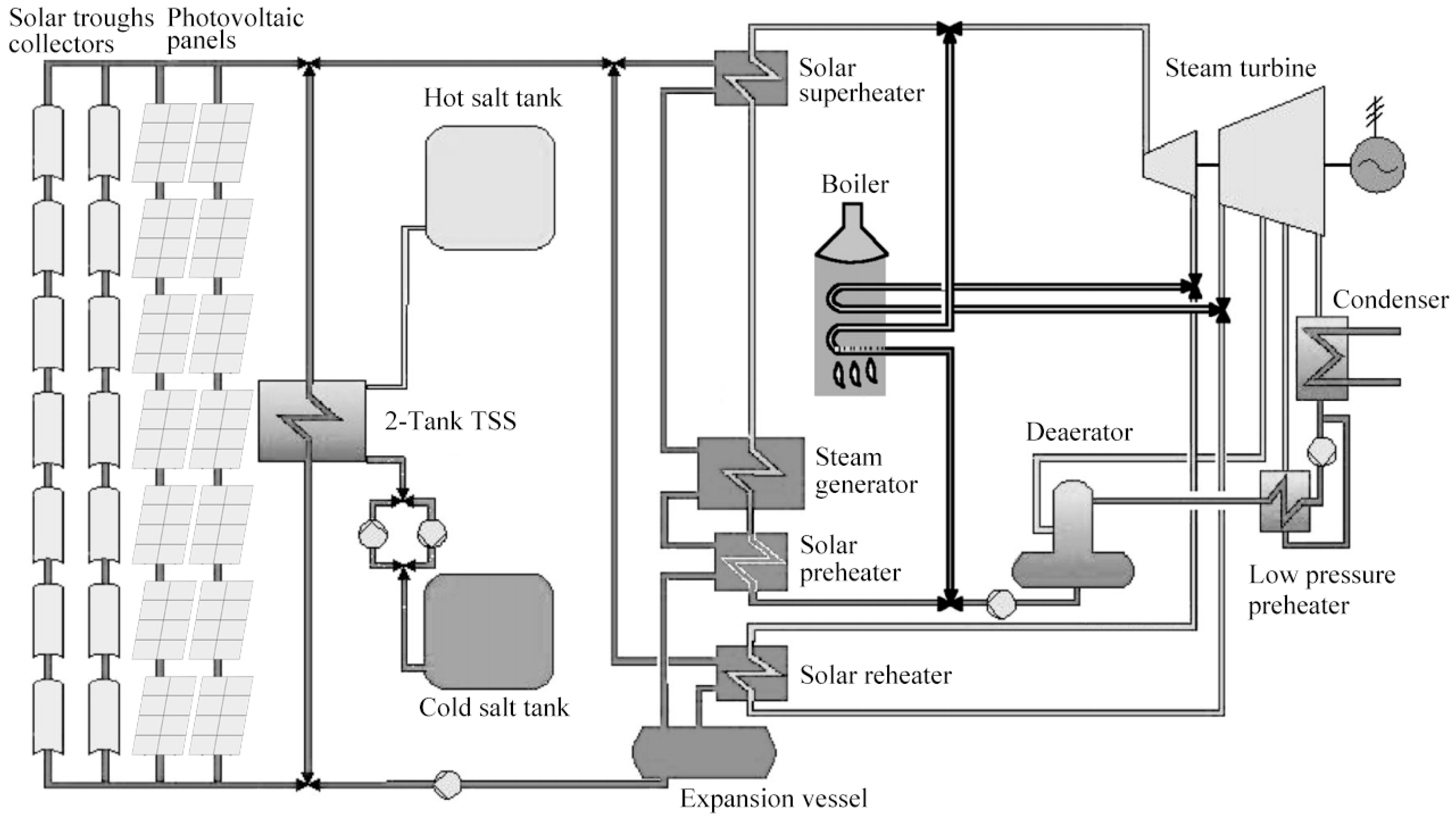
Same as photovoltaic (PV) generation, CSP units use solar energy as the primary energy source, and there is almost no carbon emission problem [16]. The difference is that the thermal energy of sunlight is utilized in CSP units to generate electricity, and the output characteristics are similar to those of conventional steam turbines, which are adjustable and have very good performance in the power ramp rate. In addition, an advantage of CSP over many renewables is that it is usually equipped with a thermal storage system (TSS), which allows 15-hour continuous full-load power generation in the absence of sunlight or other extreme cases [17]. The medium materials in a TSS are usually molten salt, with high efficiency and low cost [18].

The structure of a CSP plant is broadly described in Figure 2 [19], and consists of solar fields, a heat transfer fluid/steam generation system, a Rankine steam turbine/generator cycle, and the TSS. In this work, the solar fields are designed in a hybrid solution combining the trough collectors and panels for improving system performance during low solar radiation periods [20,21,22]. CSP plants use heat transfer fluid (HTF), mostly heat transfer oil in the existing CSP plants, to absorb radiant energy in a solar receiver. The use of molten salts and phase changing material as HTFs can effectively improve the plant energy efficiency [23,24]. In solar fields, the lower temperature oil is heated to almost 400 °C, and the collected solar energy is exchanged to the steam generator, which can produce superheated steam (10.4 MPa, 370 °C). The superheated steam is then fed to a conventional reheat steam turbine/generator to produce electricity. This heat absorbed by HTF can be used immediately to generate power or stored in the TSS for later use for power generation in off-sun hours [25].

In the past few decades there has been a spurt in research reporting interesting results on the choice of working fluids for organic Rankine cycle-based power generation [26,27,28,29]. However, the integration of a solar field with supercritical CO₂ Brayton power cycles can achieve a high level of thermal efficiency due to the high solar concentration ratio associated with solar central receiver systems [30]. When CO₂ is operated beyond its critical point (T = 304.1 K, P = 7.37 MPa), it is called supercritical CO₂ [31]. The integration of the solar field with supercritical CO₂ Brayton power cycles in CSP plants was studied in [32,33], and the applicability and efficiency were proved.

According to the estimation of the US Department of Energy, the power generation cost of a CSP plant will be as low to 0.06 $/kWh in 2020 [34]. Previous research into CSP is mainly from the perspective of its electricity generation performance, but the utilization of its thermal energy has not yet been widely addressed. Combined heat and power generation projects of CSP plants have already been carried out in Gansu Province and Tibet Province, both in western China.

Thanks to its excellent characteristics, together with large-scale TSS, CSP will play a more important role in the development of the energy internet. Thus, a new operation mode for residential energy hubs with a CSP unit inside is proposed in this paper. Solar energy and electricity from the grid are used as the energy inputs, and the residential electrical and thermal demands are satisfied. Moreover, the demand side management is considered by modeling some of the family active loads. Then, a mixed integer linear programming (MILP) model is presented with the objective of minimizing the operation cost. Finally, the proposed optimization model is solved by the commercial CPLEX solver based on the YALMIP toolbox in MATLAB, and sample examples are provided in order to demonstrate the essential features of the proposed method.

The rest of this paper is organized as follows: the components of the proposed energy hub are described in Section 2. Mathematical models of the hub as well as some of the active loads are developed in Section 3. Case studies and simulation results are discussed in Section 4. Finally, conclusions are given in Section 5.

2. The Proposed Energy Hub

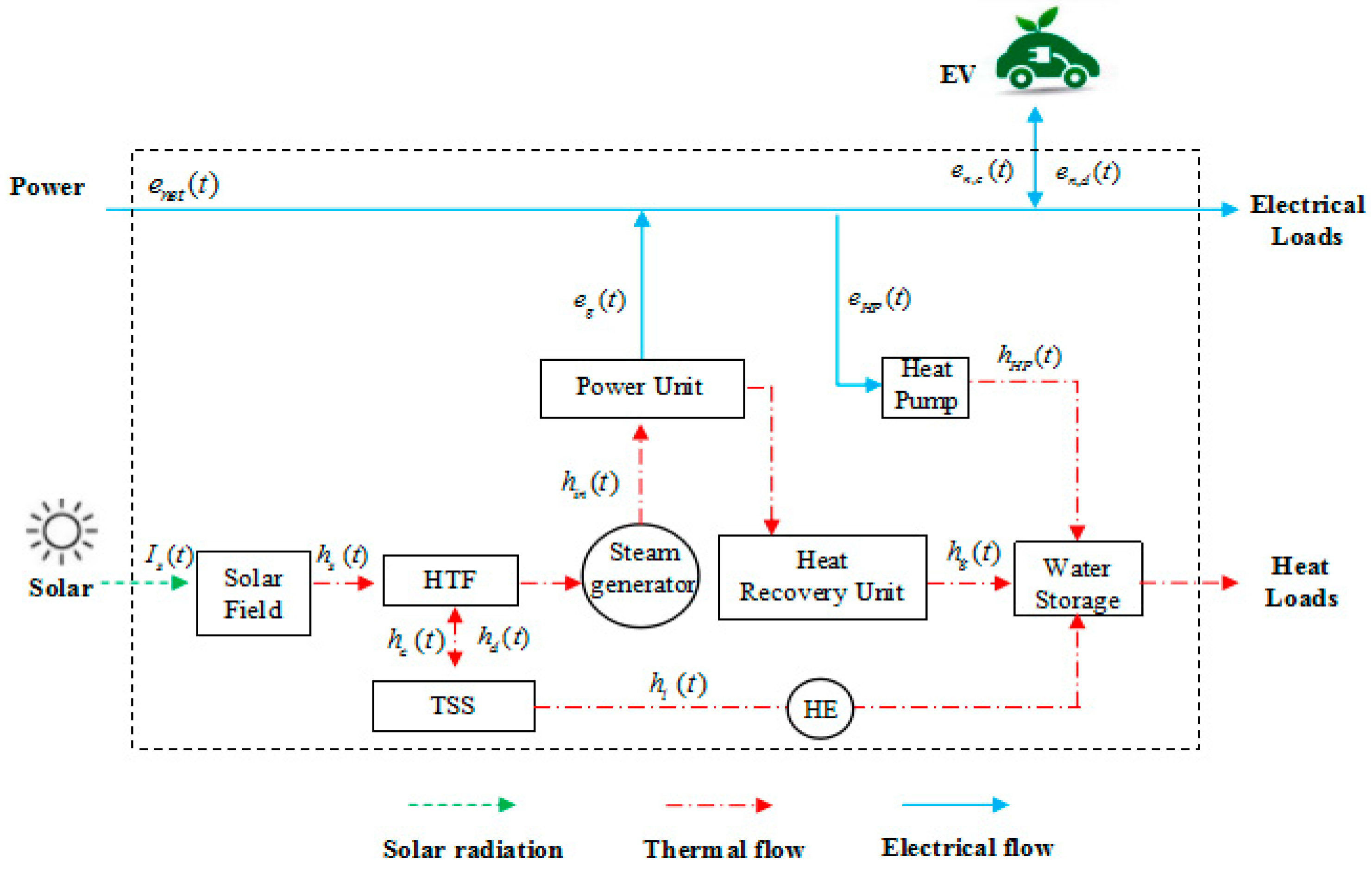
The proposed energy hub is mainly composed of the CSP unit, heat recovery unit, heat pump and water storage tank, as shown in Figure 3. Solar radiation and electricity from the main grid are used as inputs into the energy hub, and electricity demands and thermal demands are supplied through a series of energy conversion devices.

The electrical demands of users can be satisfied by the power from the grid as well as the CSP plant. However, the use of the thermal energy of the CSP plant has almost been neglected in the existing research. Similar to the CHP unit, the waste heat from the power generation unit can be utilized by adding a heat recovery unit [35]. Moreover, the thermal energy in the TSS can supply thermal demands directly for users as well, through the heat exchanger (HE).

The heat pump is driven by electrical energy [36], and attains low-level heat from air, water and soil, and supplies high-level heat to residential users. The heating efficiency ratio (thermal output/electrical input) is in the range of 3.0–4.0 when the ambient temperature is above 0 °C. Thus, the coordination of the heat pump and the heat recovery unit as well as TSS can provide a stable heat supply for users.

3. Problem Formulation

In this section, the proposed energy hub and detailed electrical and thermal loads are formulated mathematically.

3.1. Objective Function

The optimal operation model is formulated from an economic perspective [37,38,39], with the objective of minimizing the costs associated with the power generation of the CSP unit and the electricity purchased from the power network during the day. It is worth noting that the electricity can be sold back to the network when the power generated from the energy hub is redundant, and e_net(t) takes a negative value in this case. The objective function is expressed as:

$$\min {\displaystyle \sum _{t=1}^T\left[e_{net}(t)p_{net}(t)\Delta t+e_g(t)p_g(t)\Delta t\right]}$$

(1)

where e_net(t) and e_g(t) represent the power exchanged with the power network concerned and the output of a CSP unit at time t, respectively; and p_net(t) and p_g(t) represent the corresponding costs, respectively.

As it can be seen from (1), it is assumed that the price of purchasing/selling electricity from/to the main grid is always the same for each time interval, and the power generation cost of the CSP unit is simplified as a piecewise linear function.

3.2. Load Modeling

Demand side management is implemented by utilizing shiftable electrical loads and flexible thermal loads.

3.2.1. Electrical Load Modeling

(1) EV modeling. The charging load of electric vehicles (EVs) is shiftable. It is interruptible and can be dispatched flexibly in smart grid environment. Moreover, EVs can also be used as distributed energy storage devices. The energy stored in EVs can be transmitted back to the power network concerned, the so-called vehicle-to-grid (V2G) function. The constraints of EVs can be formulated as follows ($\forall n\in N_{EV}$):

$$e_{n,c}^{}(t)=x_{n,c}^{}(t)E_c^{}$$

(2)

$$e_{n,d}^{}(t)=x_{n,d}^{}(t)E_d^{}$$

(3)

$$x_{n,c}^{}(t)+x_{n,d}^{}(t)\le 1$$

(4)

$$S_{n,a}=S_n(t_{n,a})$$

(5)

$$S_{n,tg}\le S_n(t_{n,l})\le 1$$

(6)

$$S_n^{}(t)=S_n(t-1)+{\mu }_c^{EV}\frac{e_{n,c}^{}(t)}{b_n}\Delta t-\frac{e_{n,d}^{}(t)}{{\mu }_d^{EV}}\frac{1}{b_n}\Delta t$$

(7)

where e_n,c(t) and e_n,d(t) represent the charging and discharging power of an EV n at time t, respectively; x_n,c(t) and x_n,d(t) are the binary decision variables respectively used to represent the charging and discharging status of EV n at time t; E_c and E_d represent the rated charging and discharging power of an EV, respectively; S_n(t) represents the state of charge (SOC) of an EV n at time t; S_n,a and S_n,tg represent the SOC of an EV n at the arrival time t_n,a and the target SOC of an EV n at the departure time t_n,l, respectively; ${\mu }_c^{EV}$ and ${\mu }_d^{EV}$ respectively represent the charging and discharging efficiencies of EVs; and b_n represents the battery capacity of EV n.

Equations (2)–(4) represent the constraints of the charging and discharging behaviors of EVs. Equations (5) and (6) represent the SOC constraints of EVs at the arrival and departure time, respectively. The time-varying SOC of EVs is formulated as Equation (7).

(2) Washer. Some household appliances, such as washers, can be scheduled based on the electricity price variations, without causing significant discomfort to users. Suppose that smart meters [40] with a bidirectional communication capacity are installed in each house, so that the washers in each house can be dispatched based on the price signal. Moreover, the schedulable time interval T_op is defined in order to not have a big influence on the comfort level of customers [41]. The operational constraints of washers are expressed as ($\forall i\in N_w$):

$$u_i(t)-v_i(t)=x_i(t)-x_i(t-1),\forall t\in T_{op}$$

(8)

$$u_i(t)+v_i(t)\le 1$$

(9)

$${\displaystyle \sum _{t\in T_{op}}{x}_i(t)}=M_i$$

(10)

$${\displaystyle \sum _{k=t-U_i+1}^t{u}_i(k)\le x_i}(t),\forall t\in T_{op}$$

(11)

$${\displaystyle \sum _{t\notin T_{op}}{x}_i(t)}=0$$

(12)

where u_i(t), v_i(t) and x_i(t) are the binary decision variables used to represent the startup, shut down and on/off status of washer i at time t, respectively; and M_i and U_i represent the minimum operating time and minimum startup time of washer i.

Equations (8) and (9) represent the constraints of the operation status of washers. The minimum operation time for finishing a task and the minimum startup time are expressed by Equations (10) and (11), respectively.

(3) Total electrical loads. The electrical loads of the system consist of the rigid demands, which are nonshiftable and shiftable loads. Thus the electrical loads at time t can be formulated as:

$$l_e(t)=l_e^R(t)+{\displaystyle \sum _{N_w}{x}_i}(t)E_w+{\displaystyle \sum _{N_{EV}}{e}_{n,c}(t)}-{\displaystyle \sum _{N_{EV}}{e}_{n,d}}(t)$$

(13)

where l_e(t) represents the total electrical load at time t; $l_e^R(t)$ represents the rigid (nonshiftable) electrical demand at time t; and E_w represents the rated power of a washer.

3.2.2. Flexible Thermal Load

The thermal load is modeled within the context of the desired hot water temperature. Suppose that the water storage tank is always full, and this means that the volume of injected cold water is always the same as the consumed hot water at each time interval. According to the temperature-dependent model of thermal loads, presented in [42], the mathematical model of hot water is expressed by Equation (14). Moreover, regarding flexible thermal load modeling, the acceptable temperature range is defined by Equation (15).

$${\theta }_w(t+1)={\theta }_w(t)-\frac{{\theta }_w(t)-{\theta }_{cold}}{V}{V}_{cold}(t)+\frac{1}{\rho \cdot V\cdot C}{h}_w(t)\Delta t$$

(14)

$${\theta }_w^{\min }\le {\theta }_w(t)\le {\theta }_w^{\max }$$

(15)

$$l_h(t)=h_w(t)$$

(16)

where ${\theta }_w(t)$ represents the water temperature in the water storage tank at time t; ${\theta }_w^{\max }$ and ${\theta }_w^{\min }$ represent the maximum and minimum temperatures of water, respectively; ${\theta }_{cold}$ represents the temperature of cold water; V and V_cold(t) represent the volume of the storage tank and the volume of the injecting cold water at time t, respectively; ρ and C represent the density and the specific heat capacity of water, respectively; h_w(t) represents the heating power of the water storage tank at time t; and l_h(t) represents the total thermal load at time t.

3.3. Constraints

3.3.1. Electrical Constraints

$$e_{net}(t)+e_g(t)=e_{HP}(t)+l_e(t)$$

(17)

$$e_g(t)={\mu }_e{h}_{in}(t)$$

(18)

$$0\le e_g(t)\le E_g^{\max }$$

(19)

$$e_{net}(t)\le E_{net}^{\max }$$

(20)

where e_HP(t) represents the electrical input of the heat pump at time t; h_in(t) represents the thermal power input of a CSP unit at time t; ${\mu }_e$ represents the conversion efficiency from thermal power to electric power in a CSP unit [43]; $E_g^{\max }$ and $E_{net}^{\max }$ represent the maximum power output of a CSP unit and the maximum transmission power of the line, respectively.

The electrical power balance is expressed by Equation (17). The electrical output of a CSP unit is determined by Equation (18). The output limits of a CSP unit and transmission power constraints from the network are expressed by Equations (19) and (20).

3.3.2. Thermal Constraints

$$h_{HP}(t)+h_g(t)+{\mu }_{HE}{h}_l(t)=l_h(t)$$

(21)

$$h_s(t)+h_d(t)=h_{in}(t)+h_c(t)$$

(22)

$$h_s^{}(t)={\mu }_s{A}_s{I}_s(t)$$

(23)

$$h_g(t)={\mu }_h{h}_{in}(t)$$

(24)

$$h_{HP}(t)={\mu }_{HP}{e}_{HP}(t)$$

(25)

where h_HP(t) and h_g(t) represent the thermal power outputs of the heat pump and the CSP unit at time t, respectively; h_l(t) represents the thermal demand supplied by the TSS at time t; h_c(t) and h_d(t) respectively represent the injected and drawn heat from the TSS at time t; h_s(t) represents the thermal power from the solar field at time t; I_s(t) represents the solar radiation intensity at time t; and A_s represents the area of the PV array; ${\mu }_{HE}$, ${\mu }_s$, ${\mu }_h$ and ${\mu }_{HP}$ are the heat exchanger efficiency, photo-thermal conversion efficiency, thermal efficiency of a CSP unit and heating efficiency ratio of the heat pump, respectively.

Equation (21) represents the demand–supply balance of thermal power. Equation (22) represents the thermal power conservation of a CSP unit. Solar radiation power is determined by Equation (23), and the thermal output of a CSP unit and heat pump are expressed by Equations (24) and (25).

3.3.3. TSS Constraints

The TSS constraints are specially expressed in this section because TSS is relatively complex and plays an important role in the operation of the system.

$$W_h(t)=W_h(t-1)+{\mu }_c^{TSS}{h}_c^{}(t)\Delta t-\frac{h_d^{}(t)}{{\mu }_d^{TSS}}\Delta t-h_l(t)\Delta t-W_h^{loss}(t)$$

(26)

$$W_h^{loss}(t)=\gamma W_h(t)$$

(27)

$$W_h^{\min }\le W_h(t)\le W_h^{\max }$$

(28)

$$W_h^{\max }={\rho }^{FLH}\frac{E_g^{\max }}{{\mu }_e}$$

(29)

$$0\le h_c^{}(t)\le x_c^h(t)H_c^{\max }$$

(30)

$$0\le h_d^{}(t)\le x_d^h(t)H_d^{\max }$$

(31)

$$x_c^h(t)+x_d^h(t)\le 1$$

(32)

$${\displaystyle \sum _{t=1}^T\left[{\mu }_c^{TSS}{h}_c^{}(t)\Delta t-\frac{h_d^{}(t)}{{\mu }_d^{TSS}}\Delta t-h_l(t)\Delta t-W_h^{loss}(t)\right]}=0$$

(33)

where W_h(t) represents the thermal energy stored in TSS at time t; ${\mu }_c^{TSS}$ and ${\mu }_d^{TSS}$ respectively represent the thermal charging and discharging efficiencies of TSS at time t; $W_h^{loss}(t)$ represents the energy loss of TSS at time t; γ is the heat loss coefficient; $W_h^{\max }$ and $W_h^{\min }$ represent the maximum and minimum capacity limits of TSS, respectively; ρ^FLH represents the full-load hours of a CSP unit; $x_c^h(t)$ and $x_d^h(t)$ are the binary decision variables respectively used to represent the injecting and drawing status of TSS at time t; and $H_c^{\max }$ and $H_d^{\max }$ respectively represent the maximum thermal charging and discharging power of TSS.

Equation (26) represents the thermal energy conservation of TSS. Equation (27) represents the heat loss. The capacity limitation is represented by Equation (28). The maximum capacity is determined by the maximum output of a CSP unit and a full-load hour (FLH) in extreme weather conditions, which is expressed by Equation (29). The charging and discharging of thermal power constraints are represented by Equations (30)–(32). Equation (33) represents that the total amount of injected thermal energies are equal to those of the drawn energies in a dispatching cycle, guaranteeing the consistency of the energy in TSS at the beginning of each cycle.

3.4. Solving Method

The proposed cost-minimizing model of the energy hub is a mixed integer linear planning (MILP) problem. CPLEX is a mature commercial solver, and the proposed model is solved by a CPLEX solver based on the YALMIP/MATLAB toolbox.

4. Case Studies

4.1. Parameter Setting

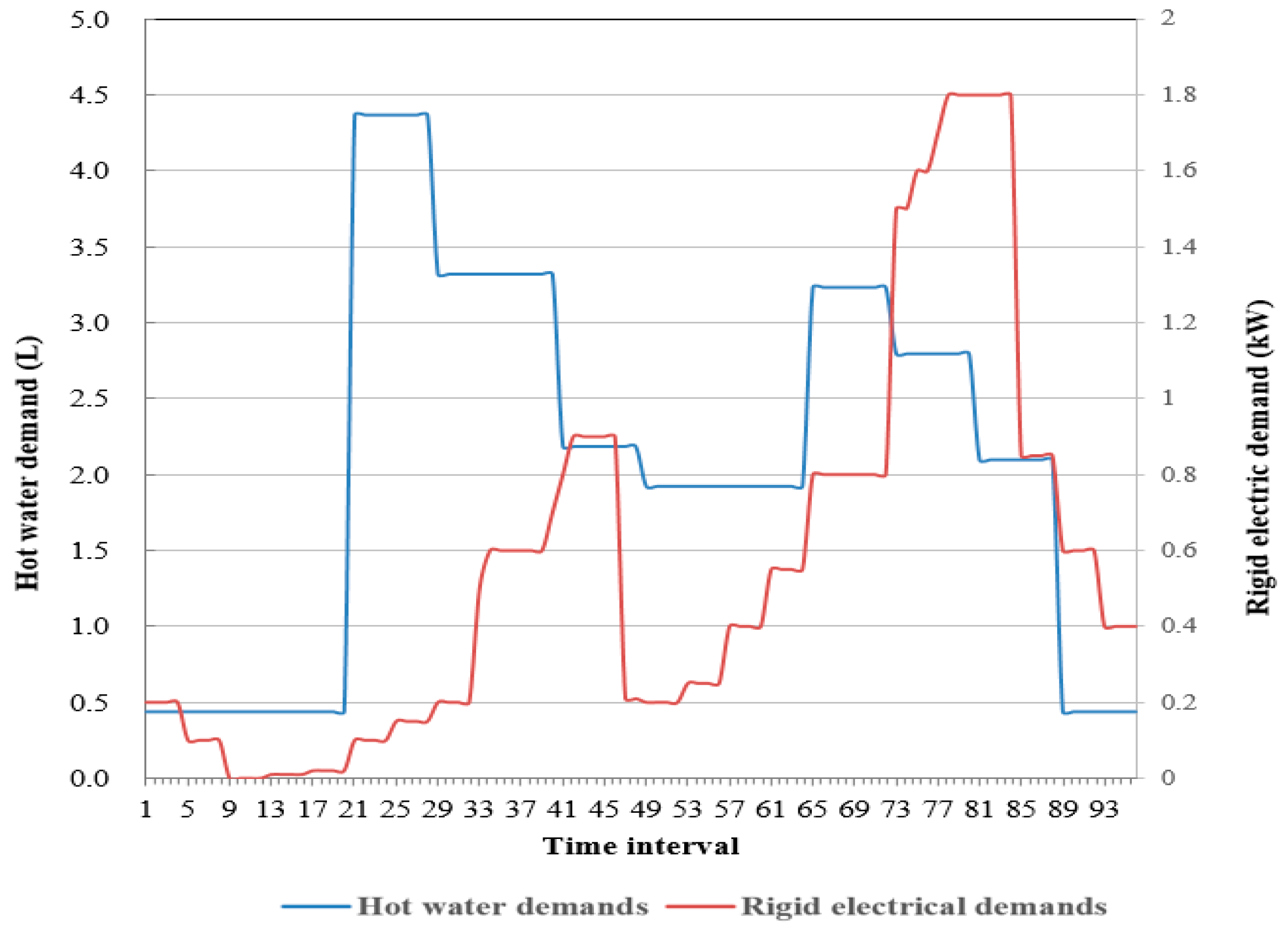
The proposed model was conducted on a residential quarter energy hub with 3000 households. A CSP power plant with a capacity of 5 MW-e was employed. The hot water demands and nonshiftable electrical demands of each household are shown in Figure 4 [44]. Suppose that each family has a washer, and the number of EVs is 1500. The arrival and departure time of the EVs follows the probability density distributions described by Equations (34) and (35) [45]. S_n,a represent random numbers distributed evenly between 10–30%. A day is divided into 96 periods in the case studies with 15 min for each time interval. It was assumed that the parameters remain unchanged in each time interval. Thus, the parameter values for this time interval can be described by the parameter values at the beginning of the period. The time-of-use (TOU) electricity prices are shown in

Table 1. Time-of-use (TOU) electricity prices.

Time	TOU	Price ($/kWh)
7:00 a.m.–8:15 a.m.	Mid-peak	0.102
8:30 a.m.–10:15 a.m.	Sub-peak	0.164
10:30 a.m.–11:30 a.m.	On-peak	0.174
11:45 a.m.–5:45 p.m.	Mid-peak	0.102
6:00 p.m.–6:45 p.m.	Sub-peak	0.164
7:00 p.m.–8:45 p.m.	On-peak	0.174
9:00 p.m.–10:45 p.m.	Sub-peak	0.164
11:00 p.m.–6:45 a.m.	Off-peak	0.041

, while other parameter assumptions are shown in

Table 2. Parameter assumption.

Parameter		Value
Rated charging and discharging power of EVs (kW)	Ec, Ed	3, 3
Rated power of a washer (kW)	Ew	0.5
Target SOC of EV n	Sn,tg	0.85
Heat loss coefficient	γ	0.01
Full-load hour (h)	ρFLH	15
Battery capacity of EV n (kWh)	bn	20
Minimum operating time of washer i (h)	Mi,	1
Minimum startup time of washer i (h)	Ui	0.25
Charging and discharging efficiencies of EVs	${\mu }_c^{EV}$,${\mu }_d^{EV}$	0.95, 0.95
Maximum and minimum temperature of the water (°C)	${\theta }_w^{\max }$,${\theta }_w^{\min }$	80, 60
Temperature of the cold water (°C)	${\theta }_{cold}$	10
Maximum power output of a CSP unit (MW)	$E_g^{\max }$	5
Maximum transmission power of the line (MW)	$E_{net}^{\max }$	2
Conversion efficiency from thermal power to electric power in a CSP unit	${\mu }_e$	0.35
Thermal efficiency of a CSP unit	${\mu }_h$	0.5
Heat exchanger efficiency	${\mu }_{HE}$	0.7
Heating efficiency ratio of the heat pump	${\mu }_{HP}$	3
Minimum capacity limit of TSS (MWh)	$W_h^{\min }$	100
Maximum thermal charging and discharging power of TSS (MW)	$H_c^{\max }$,$H_d^{\max }$	2, 2
Thermal charging and discharging efficiencies of TSS	${\mu }_c^{TSS}$,${\mu }_d^{TSS}$	0.98, 0.98

.

The variables to be optimized include the operating status of the flexible loads (e.g., EVs, washers and hot water), power exchanged with the main grid, the output of heat pumps, and the charging/discharging power of the TSS.

$$f_a(x)=\{\begin{array}{l}\frac{1}{\sqrt{2\pi }{\sigma }_a}{\mathrm{e}}^{[-\frac{{(x+24-{\mu }_a)}^2}{2{\sigma }_a{}^2}]},0\text{<}x\le {\mu }_a-12\\ \\ \frac{1}{\sqrt{2\pi }{\sigma }_a}{\mathrm{e}}^{[-\frac{{(x-{\mu }_a)}^2}{2{\sigma }_a{}^2}]},{\mu }_a-12\text{<}x\le 24\end{array}$$

(34)

where, μ_a = 17.47, σ_a = 3.41.

$$f_l(x)=\{\begin{array}{l}\frac{1}{\sqrt{2\pi }{\sigma }_l}{\mathrm{e}}^{[-\frac{{(x-{\mu }_l)}^2}{2{\sigma }_l{}^2}]},0\text{<}x\le {\mu }_l+12\\ \\ \frac{1}{\sqrt{2\pi }{\sigma }_l}{\mathrm{e}}^{[-\frac{{(x-24-{\mu }_l)}^2}{2{\sigma }_l{}^2}]},{\mu }_l+12\text{<}x\le 24\end{array}$$

(35)

where, μ_l = 8.92, σ_l = 3.24.

4.2. Simulation and Results

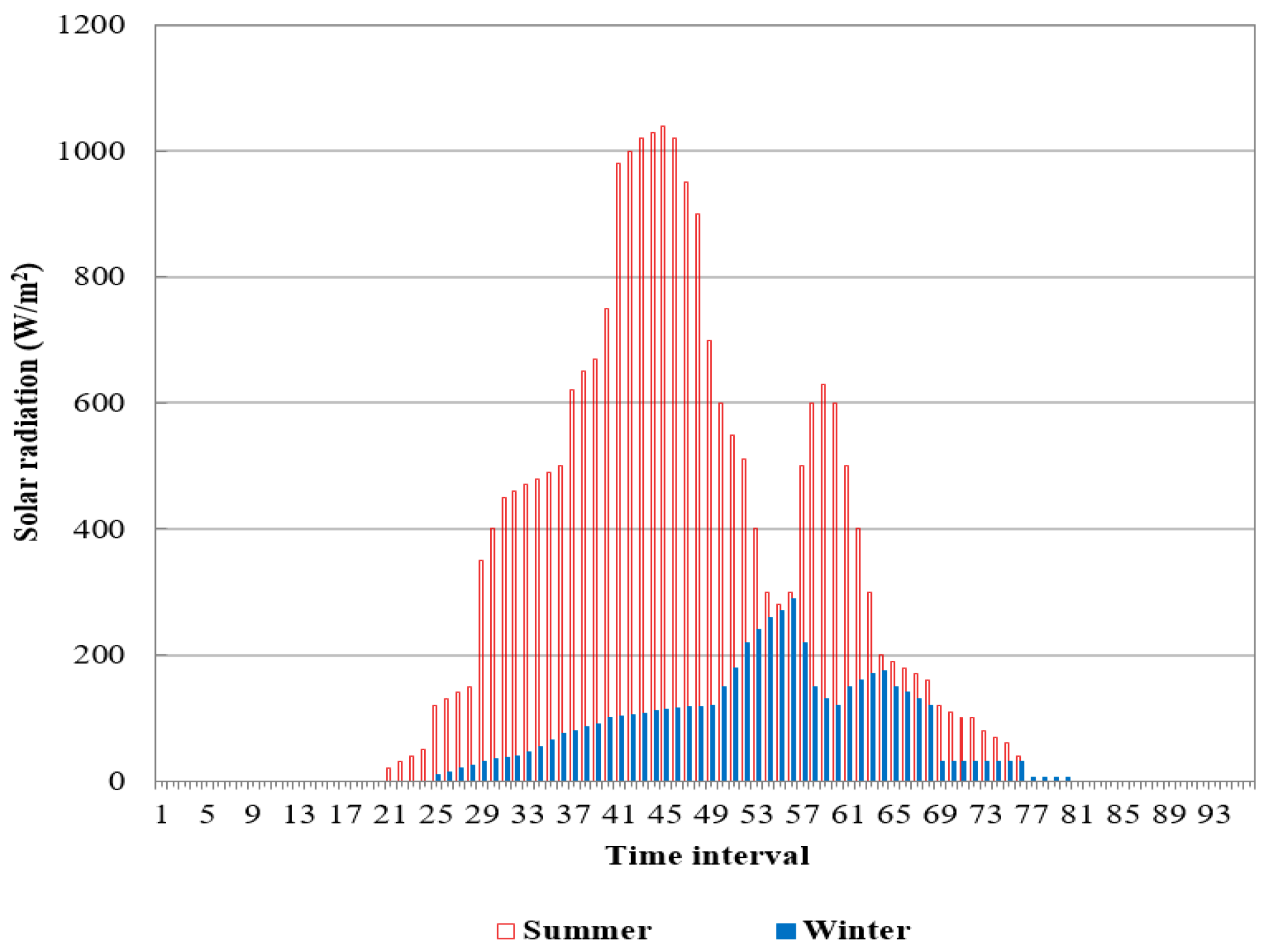
The CPLEX solver based on the YALMIP toolbox in MATLAB was employed to solve the proposed MILP model for typical summer and winter days. The solar irradiance data for a typical day in summer and in winter are shown in Figure 5, which were measured at the Center for Sustainable Energy Systems at the Australian National University [46]. The total operation costs of the energy hub were $3212.07 and $5003.48 for a typical summer day and a typical winter day according to the results, respectively. The analysis and comparison of the summer and winter cases will be presented in this section.

4.2.1. Typical Summer Day

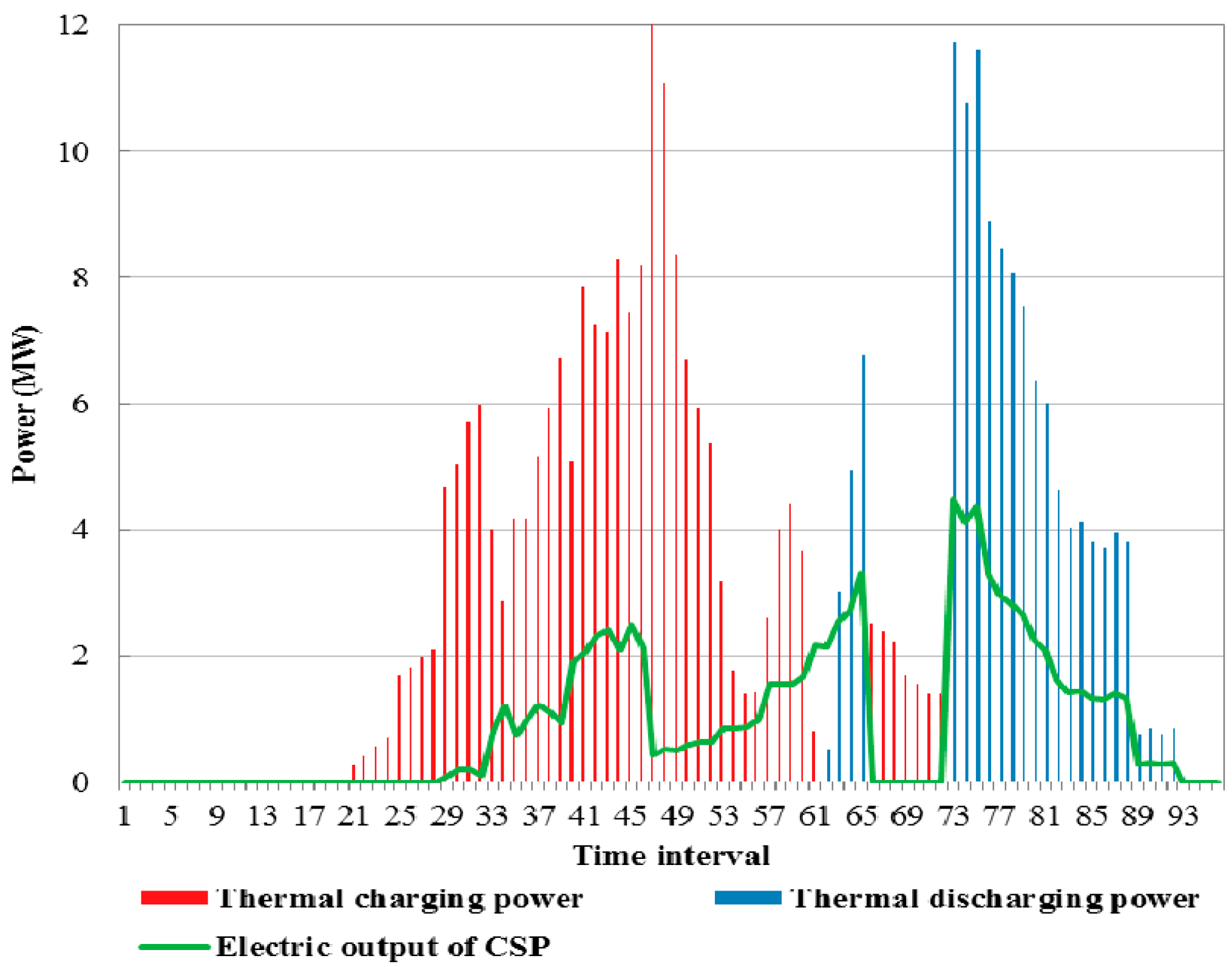
The thermal charging and discharging status of the TSS and the power generation of a CSP unit are depicted in Figure 6. The output of the CSP reached the peak in the time interval t ∈ [73, 76], during which the conventional electrical load was also close to the maximum. The optimization module responded to the change of price automatically during the day and acted in a way that mitigated the load level as much as possible during the peak-load hours with on-peak prices. Moreover, the CSP had continuous output in the time interval t ∈ [77, 92], during which the solar radiation intensity was 0 or close to 0, due to the presence of the TSS.

Figure 7 illustrates the charging and discharging power of EVs and the operation of washers. EVs discharge on a large scale in t ∈ [34, 46] and [73, 92] periods, which are the peak-price periods for electricity. In these periods, EVs discharge to satisfy the electrical demands, thus reducing the cost of electricity purchased from the power network. The charging power of EVs and working time of washers are concentrated in t ∈ [1, 28], [49, 72], and [93, 96] periods, during which the electricity prices are lower, i.e., $0.041 and $0.102, respectively. Meanwhile, as known from the rigid demand curve, the centralized discharging time of EVs is also in the peak-load periods. Thus, the introduction of shiftable loads can not only reduce the operation costs, but also plays an important load-shifting role in the system.

The heating power of water storage tanks and the hot water temperature curves are shown in Figure 8. As shown in the curves, the thermal output reaches the day’s peak in the t ∈ [73, 84] period, during which the stored water is constantly heated. The temperature reaches its maximum in the t ∈ [85, 92] period. After that, since the cost of CSP generation is greater than the electricity price, the electrical output (as well as the thermal output) of CSP is controlled to be as little as possible. The thermal energy in the TSS is utilized cooperatively to maintain the temperature of the hot water through the heat exchanger.

4.2.2. Typical Winter Day

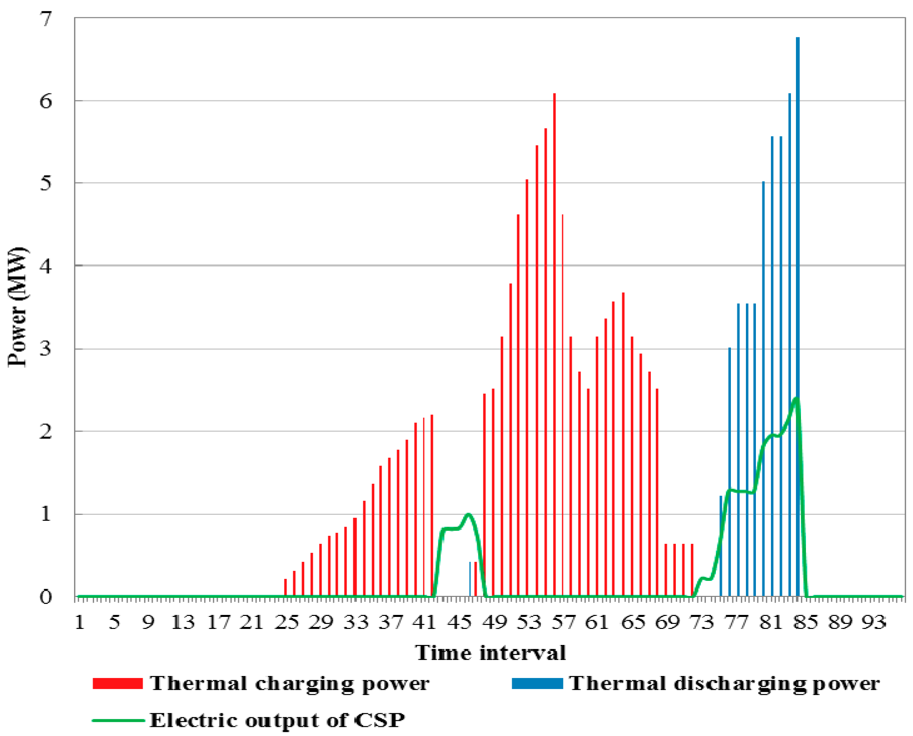
The thermal charging and discharging status of the TSS and the power generation of the CSP unit on a typical winter day are shown in Figure 9. The output of the CSP unit only rose in t ∈ [41, 47] and [73, 84] periods. The output of the CSP unit was significantly reduced due to the decrease of solar radiation intensity compared with a summer day, but still concentrated in the peak load periods. Meanwhile, the cost of the energy hub was increased obviously on winter days due to the reduced CSP output.

There is no significant difference in the behaviors of the shiftable electrical loads compared to the summer case, so they are no longer described in detail in this section. Their excellent performance, however, cannot be ignored.

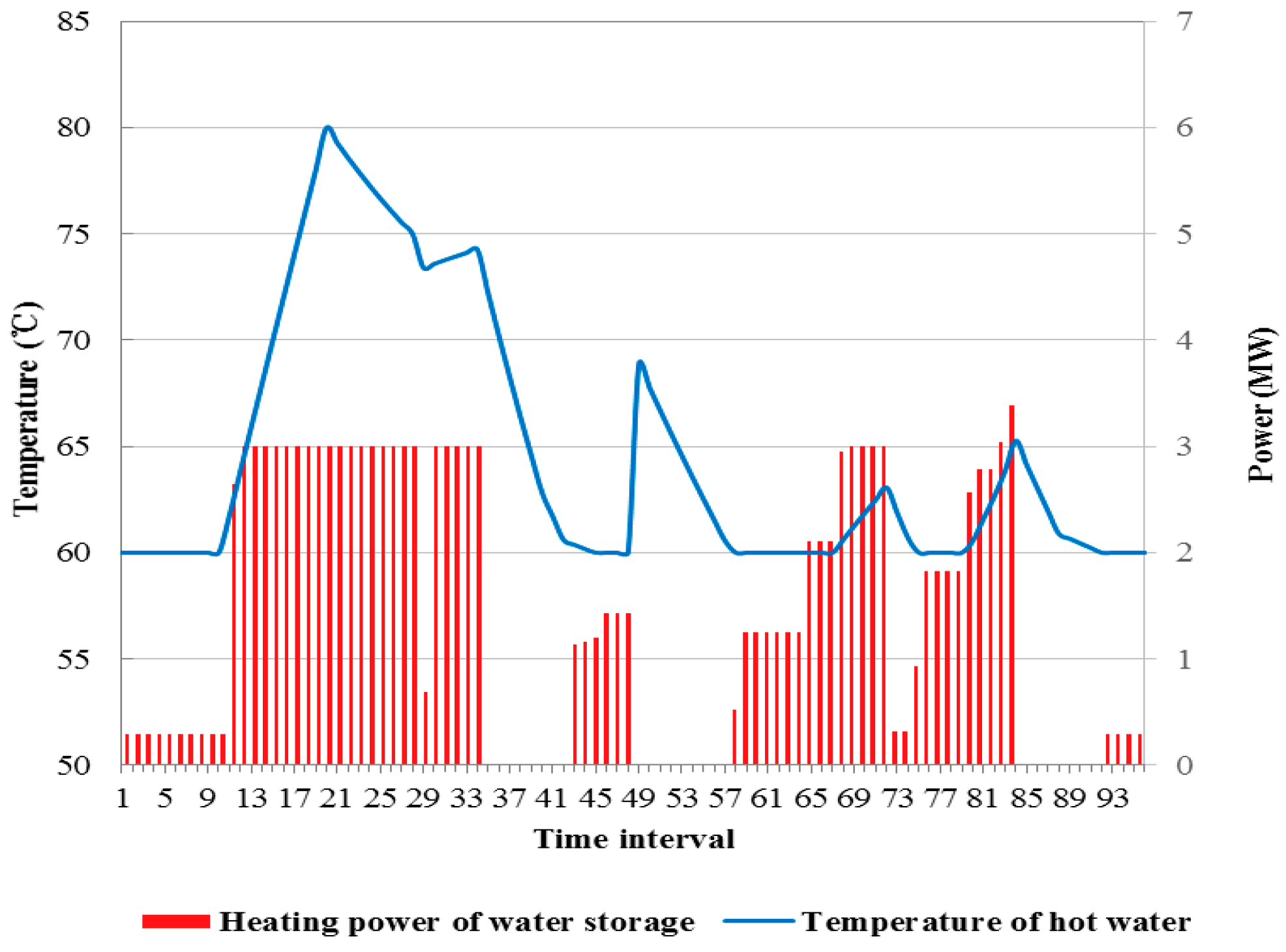
The heating power of the water storage tank and the hot water temperature curves for a typical winter day are shown in Figure 10. The thermal output was reduced due to the decrease of corresponding electrical output, so the temperature of hot water was only maintained at the pre-set minimum level most of the time. It is worth mentioning that the energy purchased from the grid were 36.16 MWh and 62.29 MWh in the summer and winter cases, respectively. Besides the reduction of CSP output, the increase of power consumption of HP, which was used to satisfy the heat demands, caused the larger amount of purchased electricity in winter. That is also an important factor in the increase of costs on a typical winter day.

Table 3. Changes of operation costs with various numbers of EVs.

Number of EVs	Cost ($)
750	5201.89
1500	5003.48
2250	4927.72

shows the changes in the operation costs of the system with the variation of EV numbers. It can be seen that the costs decrease with an increase in the numbers of EVs. The excellent cost-reduction performance of EVs for the proposed system is further demonstrated.

5. Conclusions

In this paper, a residential quarter energy hub model with a CSP unit was presented. Solar energy and electricity from the main power grid served as the inputs into the system to provide electrical and thermal loads for residential users. The demand side management was implemented by utilizing shiftable electrical loads and flexible thermal loads. Based on the proposed architecture, an MILP optimization model with the objective of minimizing the operation cost was developed, and then solved by a YALMIP/CPLEX solver. Case studies were carried out, and it was shown by simulations that the proposed model exhibits good performance in cost saving and load shifting.

The following issues will be investigated in future research efforts:

(a)

Integration strategies for biomass boilers with a CSP for backing up CSP production on winter days;

(b)

Integration strategies of CSP with wind power for enhancing the capability of accommodating wind power in the context of the emerging energy internet;

(c)

In-depth ambient temperature sensing analysis in power units for improving the overall working performance of CSP.

References

- Lorincz, J.; Bule, I.; Milutin, K. Performance analyses of renewable and fuel power supply systems for different base station sites. Energies 2014, 7, 7816–7846. [Google Scholar] [CrossRef]
- Guo, Y.; Liu, W.; Wen, F.; Salam, A.; Mao, J.; Li, L. Bidding strategy for aggregators of electric vehicles in day-ahead electricity markets. Energies 2017, 10, 144. [Google Scholar] [CrossRef]
- Yao, W.; Chung, C.Y.; Wen, F.; Qin, M.; Xue, Y. Scenario-based comprehensive expansion planning for distribution systems considering integration of plug-in electric vehicles. IEEE Trans. Power Syst. 2015, 31, 317–328. [Google Scholar] [CrossRef]
- Rifkin, J. The third industrial revolution: How lateral power is transforming energy, the economy, and the world. Survival 2011, 2, 67–68. [Google Scholar] [CrossRef]
- Krause, T.; Andersson, G.; Frohlich, K.; Vaccaro, A. Multiple-Energy carriers: Modeling of production, delivery, and consumption. Proc. IEEE 2011, 99, 15–27. [Google Scholar] [CrossRef]
- Geidl, M.; Koeppel, G.; Favre-Perrod, P.; Klockl, B.; Anderssoon, G.; Frohlich, K. Energy hubs for the future. IEEE Power Energy Mag. 2007, 5, 24–26. [Google Scholar] [CrossRef]
- Clegg, S.; Mancarella, P. Integrated modeling and assessment of the operational impact of power-to-gas (P2G) on electrical and gas transmission network. IEEE Trans. Sustain. Energy 2015, 6, 1234–1244. [Google Scholar] [CrossRef]
- Martinez-Mares, A.; Fuerte-Esquivel, C.R. A unified gas and power flow analysis in natural gas and electricity coupled networks. IEEE Trans. Power Syst. 2012, 27, 2156–2166. [Google Scholar] [CrossRef]
- Li, T.; Eremia, M.; Shahidehpour, M. Interdependency of natural gas network and power system security. IEEE Trans. Power Syst. 2008, 23, 1817–1824. [Google Scholar] [CrossRef]
- Shahidehpour, M.; Fu, Y.; Wiedman, T. Impact of natural gas infrastructure on electric power systems. Proc. IEEE 2005, 93, 1042–1056. [Google Scholar] [CrossRef]
- Li, Z.; Wu, W.C.; Shahidehpour, M.; Wang, J.H.; Zhang, B.M. Combined heat and power dispatch considering pipeline energy storage of district heating network. IEEE Trans. Sustain. Energy 2016, 7, 12–22. [Google Scholar] [CrossRef]
- Mukherjee, U.; Maroufmashat, A.; Narayan, A.; Elkamel, A.; Fowler, M. A stochastic programming approach for the planning and operation of a power to gas energy hub with multiple energy recovery pathways. Energies 2017, 10, 868. [Google Scholar] [CrossRef]
- Salimi, M.; Ghasemi, H.; Adelpour, M.; Vaez, S. Optimal planning of energy hubs in interconnected energy systems: A case study for natural gas and electricity. IET Gener. Transm. Distrib. 2015, 9, 695–707. [Google Scholar] [CrossRef]
- Zhang, X.; Shahidehpour, M.; Alabdulwahab, A.; Abusorrah, A. Optimal expansion planning of energy hub with multiple energy infrastructures. IEEE Trans. Smart Grid 2015, 6, 2302–2311. [Google Scholar] [CrossRef]
- Deng, S.; Wu, L.L.; Wei, F.; Wu, Q.H.; Jing, Z.X.; Zhou, X.X.; Li, M.S. Optimal operation of energy hubs in an integrated energy network considering multiple energy carriers. In Proceedings of the IEEE Innovative Smart Grid Technologies-Asia (ISGT-Asia), Melbourne, Australia, 28 November–1 December 2016. [Google Scholar]
- Desideri, U.; Campana, P.E. Analysis and comparison between a concentrating solar and a photovoltaic power plant. Appl. Energy 2014, 113, 422–433. [Google Scholar] [CrossRef]
- Usaola, J. Operation of concentrating solar power plants with storage in spot electricity markets. IET Renew. Power Gener. 2012, 6, 59–66. [Google Scholar] [CrossRef]
- Sioshansi, R.; Denholm, P. The value of concentrating solar power and thermal energy storage. IEEE Trans. Sustain. Energy 2010, 1, 173–183. [Google Scholar] [CrossRef]
- Price, H.; Lupfert, E.; Kearney, D. Advances in parabolic trough solar power technology. J. Sol. Energy Eng. 2012, 124, 109–125. [Google Scholar] [CrossRef]
- Madaeni, S.H.; Sioshansi, R.; Denholm, P. Estimating the capacity value of concentrating solar power plants: A case study of the Southwestern United States. IEEE Trans. Power Syst. 2012, 27, 1116–1124. [Google Scholar] [CrossRef]
- Madaeni, S.H.; Sioshansi, R.; Denholm, P. Estimating the capacity value of concentrating solar power plants with thermal energy storage: A case study of the Southwestern United States. IEEE Trans. Power Syst. 2013, 28, 1205–1215. [Google Scholar] [CrossRef]
- Domínguez, R.; Conejo, A.J.; Carrión, M. Operation of a fully renewable electric energy system with CSP plants. Appl. Energy 2014, 119, 417–430. [Google Scholar] [CrossRef]
- National Renewable Energy Laboratory (NREL). Summary Report for Concentrating Solar Power Thermal Storage Workshop: New Concepts and Materials for Thermal Energy Storage and Heat-Transfer Fluids. Available online: http://www.nrel.gov/docs/fy11osti/52134.pdf (accessed on 10 June 2017).
- Hartl, R.; Fleischmann, M.; Gschwind, R.M.; Winter, M.; Gores, H.J. A liquid inorganic electrolyte showing an unusually high lithium ion transference number: A concentrated solution of LiAlCl4 in sulfur dioxide. Energies 2013, 6, 4448–4464. [Google Scholar] [CrossRef]
- Lopes, M.L.; Johnson, N.G.; Miller, J.E.; Stechel, E.B. Concentrating solar power systems with advanced thermal energy storage for emerging markets. In Proceedings of the IEEE Global Humanitarian Technology Conference, Seattle, WA, USA, 13–16 October 2016; pp. 444–450. [Google Scholar]
- Garg, P.; Kumar, P.; Srinivasan, K. Supercritical carbon dioxide Brayton cycle for concentrated solar power. J. Supercrit. Fluid. 2013, 76, 54–60. [Google Scholar] [CrossRef]
- Papadopoulos, A.I.; Stijepovic, M.; Linke, P. On the systematic design and selection of optimal working fluids for organic Rankine cycles. Appl. Thermal Eng. 2010, 30, 760–769. [Google Scholar] [CrossRef]
- Rayegan, R.; Tao, Y.X. A procedure to select working fluids for solar organic Rankine cycles (ORCs). Renew. Energy 2011, 36, 659–670. [Google Scholar] [CrossRef]
- Angelino, G.; Paliano, P.C.D. Multicomponent working fluids for organic Rankine cycles (ORCs). Energy 1998, 23, 449–463. [Google Scholar] [CrossRef]
- Ho, C.K.; Iverson, B.D. Review of high-temperature central receiver designs for concentrating solar power. Renew. Sustain. Energy Rev. 2014, 29, 835–846. [Google Scholar] [CrossRef]
- Al-Sulaiman, F.A.; Atif, M. Performance comparison of different supercritical carbon dioxide Brayton cycles integrated with a solar power tower. Energy 2015, 82, 61–71. [Google Scholar] [CrossRef]
- Chacartegui, R.; Escalona, J.M.M.D.; Sánchez, D.; Monje, B.; Sánchez, T. Alternative cycles based on carbon dioxide for central receiver solar power plants. Appl. Thermal Eng. 2011, 31, 872–879. [Google Scholar] [CrossRef]
- Atif, M.; Al-Sulaiman, F.A. Performance analysis of supercritical CO2 Brayton cycles integrated with solar central receiver system. In Proceedings of the 2014 5th International Renew Energy Congress, Hammamet, Tunisia, 25–27 March 2014; pp. 1–6. [Google Scholar]
- National Renewable Energy Laboratory (NREL). On the Path to Sunshot: Advancing Concentrating Solar Power Technology, Performance, and Dispatchability. Available online: http://www.nrel.gov/docs/fy16osti/65688.pdf (accessed on 10 June 2017).
- Brahman, F.; Honarmand, M.; Jadid, S. Optimal electrical and thermal energy management of a residential energy hub, integrating demand response and energy storage system. Energy Build. 2015, 90, 65–75. [Google Scholar] [CrossRef]
- Guo, Y.H.; Hu, B.; Wan, L.Y.; Xie, K.G.; Yang, H.J.; Shen, Y.M. Optimal economic short-term scheduling of CHP microgrid incorporating heat pump. Autom. Electr. Power Syst. 2015, 39, 16–22. [Google Scholar]
- Hussain, A.; Bui, V.H.; Kim, H.M.; Im, Y.H.; Lee, J. Optimal energy management of combined cooling, heat and power in different demand type buildings considering seasonal demand variations. Energies 2017, 10, 789. [Google Scholar] [CrossRef]
- Liu, Y.; Gao, S.; Zhao, X.; Zhang, C.; Zhang, N.Y. Coordinated operation and control of combined electricity and natural gas systems with thermal storage. Energies 2017, 10, 917. [Google Scholar] [CrossRef]
- Macedo, L.H.; Franco, J.F.; Rider, M.J.; Romero, R. Optimal operation of distribution networks considering energy storage devices. IEEE Trans. Smart Grid 2015, 6, 2825–2836. [Google Scholar] [CrossRef]
- Han, D.M.; Lim, J.H. Smart home energy management system using IEEE 802.15.4 and zigbee. IEEE Trans. Consum. Electron. 2010, 56, 1403–1410. [Google Scholar] [CrossRef]
- Bozchalui, M.C.; Hashmi, S.A.; Hassen, H.; Canizares, C.A. Optimal operation of residential energy hubs in smart grids. IEEE Trans. Smart Grid 2012, 3, 1755–1766. [Google Scholar] [CrossRef]
- Tasdighi, M.; Ghasemi, H.; Rahimi-kian, A. Residential microgrid scheduling based on smart meters data and temperature dependent thermal load modeling. IEEE Trans. Smart Grid 2014, 5, 349–357. [Google Scholar] [CrossRef]
- He, G.; Chen, Q.; Kang, C.; Xia, Q. Optimal offering strategy for concentrating solar power plants in joint energy, reserve and regulation markets. IEEE Trans. Sustain. Energy 2016, 7, 1245–1254. [Google Scholar] [CrossRef]
- Zhang, H.; Wen, F.; Zhang, C.; Meng, J.; Lin, G.; Dang, S. Optimal optimization model of home energy hubs considering comfort level of customers. Autom. Electr. Power Syst. 2016, 40, 32–39. [Google Scholar]
- Yao, W.F.; Zhao, J.H.; Wen, F.S.; Xue, Y.S. A hierarchical decomposition approach for coordinated dispatch of plug-in electric vehicles. IEEE Trans. Power Syst. 2013, 28, 2768–2778. [Google Scholar] [CrossRef]
- Tushar, W.; Yuen, C.; Huang, S.S.; Smith, D.B.; Poor, H.V. Cost minimization of charging stations with photovoltaics: An approach with EV classification. IEEE Trans. Intell. Transp. Syst. 2015, 17, 156–169. [Google Scholar] [CrossRef]
Figure 1.
An illustrative energy hub.
Figure 2.
The overall structure of a concentrating solar power (CSP) plant.
Figure 3.
The proposed residential quarter energy hub model.
Figure 4.
Daily hot water demands and rigid electrical demands for a single residential consumer.
Figure 5.
The solar radiation curves.
Figure 6.
Thermal charging/discharging power and the electrical output of a CSP unit on a typical summer day.
Figure 7.
Shiftable electrical loads on a typical summer day.
Figure 8.
Heating power of the water storage tank and the temperature of hot water on a typical summer day.
Figure 9.
Thermal charging/discharging power and the electrical output of a CSP unit on a typical winter day.
Figure 10.
Heating power of the water storage tank and the temperature of hot water on a typical winter day.