Microgrid-Level Energy Management Approach Based on Short-Term Forecasting of Wind Speed and Solar Irradiance


Computer Engineering Department, College of Computer and Information Sciences, King Saud University, Riyadh 11543, Saudi Arabia
*
Author to whom correspondence should be addressed.
Energies 2019, 12(8), 1487; https://doi.org/10.3390/en12081487
Submission received: 15 January 2019
/
Revised: 8 April 2019
/
Accepted: 11 April 2019
/
Published: 19 April 2019
(This article belongs to the Special Issue Ensemble Forecasting Applied to Power Systems)
Abstract
:Background: The Distributed Energy Resources (DERs) are beneficial in reducing the electricity bills of the end customers in a smart community by enabling them to generate electricity for their own use. In the past, various studies have shown that owing to a lack of awareness and connectivity, end customers cannot fully exploit the benefits of DERs. However, with the tremendous progress in communication technologies, the Internet of Things (IoT), Big Data (BD), machine learning, and deep learning, the potential benefits of DERs can be fully achieved, although a significant issue in forecasting the generated renewable energy is the intermittent nature of these energy resources. The machine learning and deep learning models can be trained using BD gathered over a long period of time to solve this problem. The trained models can be used to predict the generated energy through green energy resources by accurately forecasting the wind speed and solar irradiance. Methods: We propose an efficient approach for microgrid-level energy management in a smart community based on the integration of DERs and the forecasting wind speed and solar irradiance using a deep learning model. A smart community that consists of several smart homes and a microgrid is considered. In addition to the possibility of obtaining energy from the main grid, the microgrid is equipped with DERs in the form of wind turbines and photovoltaic (PV) cells. In this work, we consider several machine learning models as well as persistence and smart persistence models for forecasting of the short-term wind speed and solar irradiance. We then choose the best model as a baseline and compare its performance with our proposed multiheaded convolutional neural network model. Results: Using the data of San Francisco, New York, and Los Vegas from the National Solar Radiation Database (NSRDB) of the National Renewable Energy Laboratory (NREL) as a case study, the results show that our proposed model performed significantly better than the baseline model in forecasting the wind speed and solar irradiance. The results show that for the wind speed prediction, we obtained 44.94%, 46.12%, and 2.25% error reductions in root mean square error (RMSE), mean absolute error (MAE), and symmetric mean absolute percentage error (sMAPE), respectively. In the case of solar irradiance prediction, we obtained 7.68%, 54.29%, and 0.14% error reductions in RMSE, mean bias error (MBE), and sMAPE, respectively. We evaluate the effectiveness of the proposed model on different time horizons and different climates. The results indicate that for wind speed forecast, different climates do not have a significant impact on the performance of the proposed model. However, for solar irradiance forecast, we obtained different error reductions for different climates. This discrepancy is certainly due to the cloud formation processes, which are very different for different sites with different climates. Moreover, a detailed analysis of the generation estimation and electricity bill reduction indicates that the proposed framework will help the smart community to achieve an annual reduction of up to 38% in electricity bills by integrating DERs into the microgrid. Conclusions: The simulation results indicate that our proposed framework is appropriate for approximating the energy generated through DERs and for reducing the electricity bills of a smart community. The proposed framework is not only suitable for different time horizons (up to 4 h ahead) but for different climates.
1. Introduction
The ongoing depletion of fossil fuels, the changing weather, and ecological pollution are some reasons for incorporating DERs into existing power systems. Many advanced countries in the world have directives for energy-providing companies to escalate their energy production from renewable energy sources. In this regard, the government of California established its Renewable Portfolio Standard (RPS) program. In this program, the government signed a bill with utilities to increase the renewable energy production from 20% in 2010 to 33% in 2020 [1].
Table 1 below shows the list of abbreviations used in this paper.
The energy generation from the DERs is intermittent in nature as it is dependent on naturally varying climate factors, such as wind speed, solar irradiance, and air temperature [2]. These atmospheric variations result in significant changes in the energy generated through DERs, which in turn leads to uncertainty. Consequently, precise and accurate prediction models are crucial for forecasting the generated energy through DERs. These models will be helpful in forecasting the generated energy through DERs, which will be available to the microgrids of smart communities. This will not only help in fulfilling energy requirements but also assist in decreasing energy costs and ensuring the adequate comfort of users in the smart community.
Owing to the intermittent nature of renewable energy resources, the development of a precise and accurate model has become an important factor for increasing the dissemination of DERs in existing power systems. Accurate forecasting of the energy generated through DERs not only helps in the incorporation of renewable energy into power systems but also guarantees good trading performance of renewable energy in the global market [3]. Nevertheless, the forecasting accuracy is heavily dependent on the atmospheric circumstances of the geographical location [4]. Thus, it becomes even more challenging.
There are two main classes of prediction models for forecasting the wind speed and solar irradiance: physical (numerical) models and machine learning (data-driven) models. The main purpose of these models is to forecast wind speed and solar irradiance for a specific location at a selected future time frame. The data-driven models are largely founded on time-series analyses [5]. Their computational complexity is lower than that of the physical models, and they are suitable for short-term prediction. On the other hand, the physical models are based on mathematical equations for relating the dynamics and the physics of the atmosphere, which influences radiation from the sun [1,3,6]. Physical models are usually used for long-term and medium-term forecasting. Consequently, in this work, we selected data-driven models for short-term forecasting owing to their lower complexity and good prediction accuracy.
In the past, traditional statistical approaches have been extensively explored for time-series analyses. Recently, machine learning and deep learning approaches have gained much attention from the research community. Artificial Neural Networks (ANNs) possess exceptional nonlinear mapping and robust generality abilities; thus, these networks can be applied to wind and solar energy forecasting [7]. However, ANN-based models easily fall into local minima and show poor generalization. Moreover, they are well known to over-fit and they have slow convergence rates [8]. In the literature, several other models have been applied, including the Extreme Learning Machine Neural Network (ELMNN) [9], Generalized Regression Neural Network (GRNN) [10], and Support Vector Machine (SVM) [11]. The performance of ELMNN heavily depends on the activation function. If the activation function is not selected appropriately it would result in the generalization degradation phenomenon [12]. Moreover, it is not suitable for applications that require deep extraction of features as it cannot encode more than one layer of abstraction. The main disadvantage of GRNN models is their size and huge computational time [13]. The SVM algorithms have some limitations, such as optimal choice of kernel, computational complexity of the model, and large memory space requirement [14].
Recently, researchers who are applying machine learning models as a core forecasting model have advanced their research with other methods, including weather categorizations [15], parameter or feature selection [16,17,18], and decorrelation [19]. Some other researchers used hybrid models to enhance the prediction precision. However, the long training time based on increased computational complexity of such models is an issue that needs consideration from the researchers. In a previous study [20], the authors explored an approach for predicting one-day-ahead PV power using neural networks and time-series analysis. The authors in another study [21] implemented and evaluated an optimized prediction model that was based on ANNs and a genetic algorithm (GA). The authors in yet another study [22] explored four architectures (Adaptive Neuro Fuzzy Inference System (ANFIS), Multilayer Perceptron (MLP), GRNN, and Nonlinear Autoregressive Recurrent Exogenous Neural Network (NARX)) for enhancing the prediction precision. They proposed hybrid wavelet-ANN models for solar forecasting at a specific site. However, the model was not tested at different geographical locations to assess the wider potential. Moreover, very limited set of features were used to train the model.
Currently, the convolutional neural network (CNN)-based model is one of the most successful models in deep learning and has been broadly adopted in different applications, including image recognition and classification, object detection, and tracking. However, CNN models have not been extensively explored in time-series analysis. The rapid progress in the computational power of hardware in the last decade has enabled CNN-based models to deeply penetrate various fields. The authors in a previous study [23] proposed a CNN model for interpreting weather data by considering the temporal and spatial associations between the independent parameters for producing local forecasts. They compared the performances of various architectures and stated that the purpose of their exploration was to show that CNN-based models can learn certain patterns of meteorological parameters and relate them to rainfall events. The authors in a previous study [24] also applied a CNN-based model for precipitation prediction.
The authors in a previous study [25] developed a hybrid model by combining long short term memory (LSTM) and CNN models for the prediction of extreme rainfall. The weather parameter was applied as an input to the CNN model, and the outputs of the CNN model were presented as inputs to the LSTM model. In this developed model, the researchers considered the LSTM and CNN models as independent steps. Atmospheric variables, including pressure and temperature, were used as input data. The authors in a previous study [26] developed a framework for the accurate forecasting of short-term wind speed. Their framework was based on hybrid nonlinear/linear models and empirical mode decomposition (EMD). They applied EMD to decompose the wind speed data into residuals and intrinsic mode functions (IMFs). They studied different linear and nonlinear models, including CNN, to analyze the residuals and the IMFs. Among all the hybrid models, EMD-ARMIA-RF performed well for ten-min-ahead forecasting. However, none of the hybrid models performed well 1 h ahead.
In the literature, an approach called benchmarking is mostly used for comparison with the newly developed algorithm [8,27]. The best existing machine learning techniques are selected and evaluated to select the baseline model. The selected baseline model is then used to compare the performance of the newly developed technique. In a previous study [28], authors compared their proposed model for short-term wind speed forecasting with commonly used machine learning algorithms, such as SVM, random forest (RF), and decision tree (DT). We have selected well-known machine learning models, including k-nearest neighbors (KNN), gradient boosting, extra tree regressor, and random forest regressor, for short-term forecasting of wind speed. The best model among them is selected as a baseline model for comparing and evaluating the performance of the proposed model.
Each of the selected machine learning models has its own limitations. For example, KNN algorithm is very sensitive to outliers, as it chose neighbors based on distance criteria. Moreover, it is computationally extensive when the dataset is very large. Gradient boosting models are sensitive to overfitting if the data is noisy. Also, they are harder to tune than other models. One of the weaknesses of random forest and extra tree models when used for regression problems is that the model cannot predict beyond the range in the training data.
Various studies confirm that physical models, such as NWP, are best suited for forecasting more than 4 h to several days [28,29,30,31,32,33,34,35]. These techniques are weak at handling smaller scale phenomenon and are not suitable for short-term forecast horizons [29]. Machine learning methods give the best results for forecast horizons of up to 6 h [30]. The choice of model depends on the forecast horizon. The NWP models generally outperform machine learning models over longer horizons. However, for short-term horizons the time series models have more power [34]. At the intra-hour forecast horizon, NWP is extremely expensive and not practical, especially for the renewable energy sector [36].
In a previous study [37], the authors used smart persistence model as a baseline for the deterministic forecast. In fact, California Independent System Operator (CAISO) uses persistence method in its renewable energy forecasting and dispatching [38]. This method is highly effective in short term prediction, i.e., 1 h ahead. It is often used as a comparison with other advanced methods [39]. In the irradiance forecasting community, numerous works have been devoted recently to the development of models that generate deterministic or point forecasts [34,40,41,42,43,44,45]. In this work, as we are dealing with short-term forecasting of solar irradiance, we have considered the persistence model and smart persistence model for comparison purposes.
We studied the trends of adaptation of the renewable energy resources in various states of the United States of America (USA). We found that California has made effective policies for the integration of renewable energy resources. In California in 2017, 32% of the electricity was acquired from renewable energy sources, due to which it seems to be well on track to meet its renewable energy targets of 33% and 50% for 2020 and 2030, respectively [46]. Based on the planned effective and concrete policies of the government of California, we have selected San Francisco from the NSRDB of the NREL as a case study in our analysis. The NSRDB uses a physics-based modeling approach, in which the solar radiation data for the entire United States is gridded into segments of 4 km × 4 km using geostationary satellites. The temporal resolution of the data is 30 min [47]. The NSRDB’s physics-based, gridded data collection approach is called the Physical Solar Model (PSM). More details about the PSM can be found in a previous study [48].
This paper proposes a multiheaded convolutional neural network (MH-CNN) model for the short-term forecasting of solar irradiance and wind speed to approximate the energy generated through solar panels and wind turbines, respectively. We consider several machine learning models, as well as persistence and smart persistence models for forecasting the short-term solar irradiance and wind speed. We then choose the best model as a baseline and compare its performance with our proposed MH-CNN model. The comparison is based on evaluation metrics, including the root mean square error (RMSE), mean absolute error (MAE), and symmetric mean absolute percentage error (sMAPE). Using the NSRDB of the NREL data of San Francisco as a case study, the results show that our proposed model outperforms all other models in forecasting the wind speed and solar irradiance. The obtained results indicate that our proposed framework for microgrid-level energy management is appropriate for approximating the renewable energy and for reducing the electricity bills of a smart community. The main contributions of our work are as follows:
- We formulated a solar irradiance and wind speed prediction problem for approximating the generated energy through solar panels and wind turbines.
- We evaluated the performance of various machine learning models, as well as persistence and smart persistence models, for selecting a baseline model.
- We proposed an MH-CNN model for the short-term forecasting of solar irradiance and wind speed.
- We evaluated the effectiveness of proposed model on different time horizons (up to 4 h).
- We evaluated the effectiveness of proposed model on different climates.
- We proposed a framework for microgrid-level energy management for reducing the electricity bills of a smart community.
The remainder of the paper is organized as follows. The related work from the literature is reviewed and presented in Section 2. The proposed framework is elaborated in Section 3. A performance evaluation of the various considered models is provided in Section 4. Results and discussions are provided in Section 5. The contributions of the paper are discussed in Section 6.
2. Related Work
Researchers from academia and industry have explored methods and technologies for tackling the problems of global energy crises. In this part of the manuscript, we present recent research work on global energy crises and explored solutions. The future Smart Grid (SG) will be composed of the latest technologies and will significantly improve the existing power grids. The possibility of two-way information flow and interoperability between smart homes provides a chance to optimize the power consumption of the end users and simultaneously improve the operation of the SG [49,50,51,52]. The increasing diffusion of renewable energy in power systems has given rise to the concept of microgrids, which will probably play a substantial role in the development of SGs [53,54]. It is anticipated that the network of microgrids will result in the formation of an SG [54]. The microgrid is composed of DERs, power loads, and Energy Storage Systems (ESS) [55,56].
Typically, DERs, such as wind turbines and solar panels, are among the useful energy resources for solving energy shortfalls. These resources also help in decreasing the effects of carbon emissions in the modern world. By incorporating DERs in power systems, consumers will be able to achieve their power requirements by generating green energy, which in turn will lead to electricity bill reductions. In the last decade, many researchers focused their efforts on solving the challenges of DERs—their integration into the SG, intermittent nature, the optimal power flow, etc. One of the important issues with the energy generated through DERs is the intermittent nature of these power-generating sources. Many researchers have dedicated their efforts to mitigating these issues [57,58]. The development of an accurate prediction model for forecasting the wind energy and solar energy is desirable. However, the generated energy from DERs is heavily reliant on the accuracy of the weather prediction model.
The accuracy of the weather prediction model is reliant on different atmospheric phenomena, such as pressure, temperature, wind speed, and humidity. The enormously random variations of weather conditions lead to difficulties in the accuracy of the prediction [58]. Fortunately, different parameters of the weather can be predicted with significant accuracy by developing any of the latest models, including the ANN, Deep Neural Network (DNN), and LSTM [59,60,61].
The authors investigated the integration of DERs in power systems in a previous study [62]. They suggested dealing with the uncertainty of DERs by virtualization, and validated their method by performing real-time experiments. The authors in another study [63] investigated a prediction model for approximating the quantity of solar energy generation. Their prediction model was composed of a wavelet transform and a neural network. They used RMSE and MAE to evaluate their developed model. A comparison of their obtained results with existing promising results proved that their developed model achieved good performance.
Recently, in a previous study [64], we proposed a short-term load prediction technique based on support vector quantile regression. In this study, we compared three kernel functions: Gaussian kernel, linear kernel, and polynomial kernel. The predicted precision of the power load was approximated using data sets from Singapore. We achieved better results compared to those from Support Vector Regression and the Firefly Algorithm. Power systems in today’s world are being transformed into distributed energy resources. The integration of DERs in existing power systems leads to energy management problems because these energy resources produce power in nondeterministic manners. The well-known “duck curve” problem arises in the off-peak hours because of the overgeneration from DERs that causes generator units to be underloaded [65]. The underloading of a generator impacts the individual components of a power system and the overall system performance because of the mismatch between generation and demand.
Recently, in a previous study [66], we considered the radial structure of a distribution grid and applied commonly used configuration topology for the integration of DERs and ESSs in power systems. Furthermore, we addressed a multilevel Multi Agent System (MAS) optimization framework for the co-scheduling of demand and supply resources. The MAS structure permits Plug-and-Play (PnP) capabilities and flexible control of DERs for load balancing. During both off-peak and peak hours, the PnP algorithm deactivates or activates the ESS to rectify demand and supply mismatches. The ESS stocks the excess energy from DERs and uses it to meet the energy demand at a later time. Our main objective has been to reduce electricity bills without compromising user comfort during peak hours. Our simulation results proved that our developed MAS helped in balancing the load while maintaining adequate user comfort.
In the current work, our aim is to develop an MH-CNN model for the short-term forecasting of wind speed and solar irradiance. The forecasted wind speed and solar irradiance will be used for approximating the generated power through wind turbines and solar panels. We performed extensive simulations to prove the improved performance of the proposed strategy. Moreover, we proposed a framework for microgrid-level energy management for reducing the electricity bills of the smart community.
3. Proposed System Model
In this section, the proposed system model is explained. It is always beneficial to reduce the electricity bill of the users without affecting their comfort. Integrating DERs in the power system helps to reduce electricity bills, increase user comfort, and fulfill energy requirements. Sometimes the total electricity generated by DERs during off-peak hours exceeds the demand of the consumer, which results in a generation-demand imbalance. The consequence of a generation-demand imbalance is the basis of the “duck curve” problem [65]. Temporarily, excessive electricity generation from DERs lessens the power load on the grid generators. In this situation, the excess power generated by the DERs may be harmful to the generator and motors. Thus, there is a need to develop efficient machine and deep learning models to accurately predict short-term renewable energy generation. Based on these models, efficient energy management frameworks need to be explored.
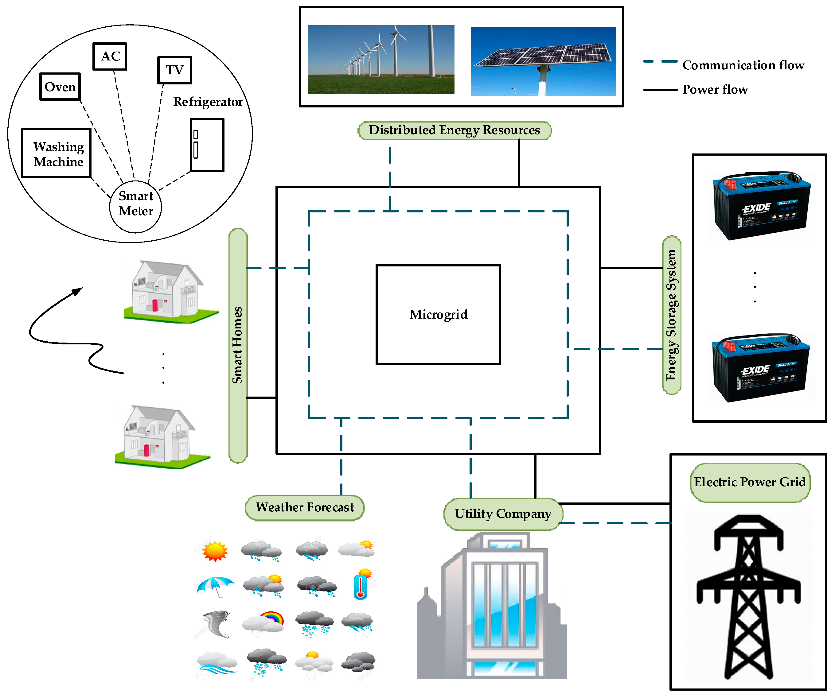
The proposed microgrid-level energy management framework is presented in Figure 1, where a smart meter, ESS, and DERs are integrated. As shown in Figure 1, an ESS is integrated in the proposed system to mitigate the influence of the duck curve problem, which we recently targeted in a previous study [66]. The smart meters are used for two-way communication in addition to many other advanced features. The DERs in the form of wind turbines and solar panels are used to generate the renewable energy to ensure the required user comfort and to reduce electricity bills. The ESSs are used for storing the excess generated energy at any time. This excess energy can then be used at a later time. In addition to DERs, the microgrid has access to power from the main grid, as the nature of the DER is intermittent and may produce very low energy on certain days and at certain times.
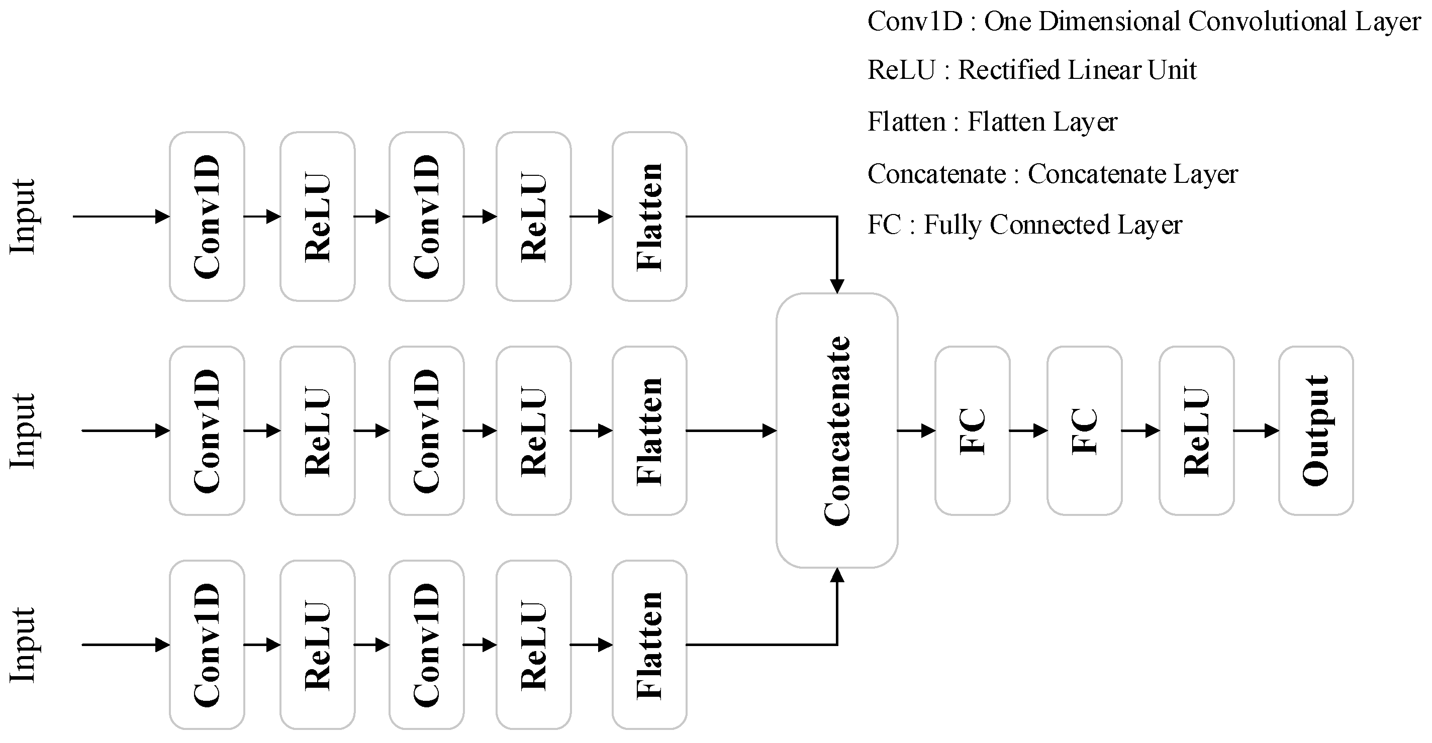
The architecture of the proposed MH-CNN model is shown in Figure 2. We used the same model for the short-term forecasting of both wind speed and solar irradiance. Meteorological parameters, such as temperature, pressure, and wind speed, as well as cyclic parameters, such as season, month, day of the year, and hour over the past day, are passed to both the wind speed and solar irradiance forecasting models. Moreover, we incorporate the past day’s lag of wind speed and solar irradiance as lag features in the wind speed and solar irradiance forecasting models, respectively. The data preparation steps are presented in Figure 3.
The same input is passed to three 1D CNNs. Each CNN has the same filter size but different kernel sizes. All three sub-CNN models extract features by looking at the input data from different aspects owing to the different kernel sizes. For our model, we used a Rectified Linear Unit (ReLU) as an activation function, as it does not encounter the gradient vanishing problem and performed best in the case study data. The CNN part consists of two 1D convolution layers. In the second convolution layer, we halved the filter size and doubled the kernel size to reduce the dimensionality and enhance the feature selection domain, respectively. The output of the second convolution layer (after applying the ReLU activation function) for each sub-CNN model is flattened and concatenated as a single feature vector. The feature vector then goes through the fully connected architecture and the ReLU activation function to produce the output, as shown in Figure 2.
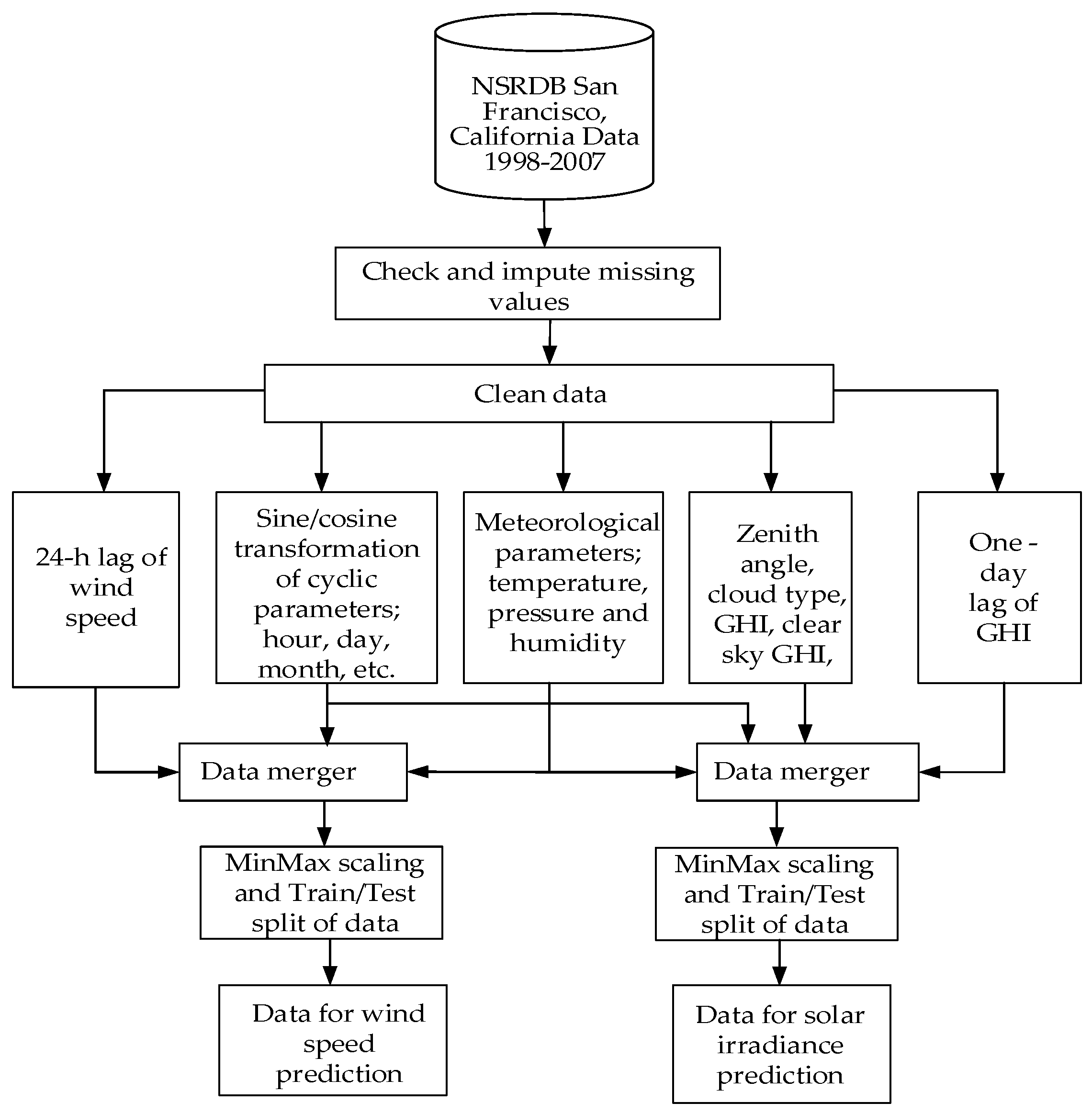
The data preprocessing steps are shown in Figure 3. Initially, the missing values are determined and are replaced with the values from the same time on the previous day. If the value from the same time of the previous day is also missing, then the missing data is imputed by using the value of the same time of the last previous day with available data. Then, further processing is performed on the clean data in three different ways. The sine and cosine transformations of cyclic parameters, such as hour of day, day of the year, month of the year, season of the year, and wind direction, are determined. We used binary encoding to encode the categorical feature named “cloud type”. This feature was obtained by the NREL from the pathfinder atmospheres extended (PATMOS-X) model. Meteorological parameters, including temperature, pressure, and wind speed, are separated. The one-day time lags of the wind speed and solar irradiance are arranged as separate features for the wind speed and solar irradiance models, respectively. These features are merged, and then normalization is performed, i.e., the range of each input vector is restricted to (0, 1). The scaled data are then separated into train and test data sets for training and evaluating the proposed model, respectively.
3.1. Convolutional Neural Networks
In this section, we describe the layers associated with the implementation of our forecasting model, including 1-D convolution, ReLU, dropout, and fully-connected layers.
3.1.1. The 1-D convolution
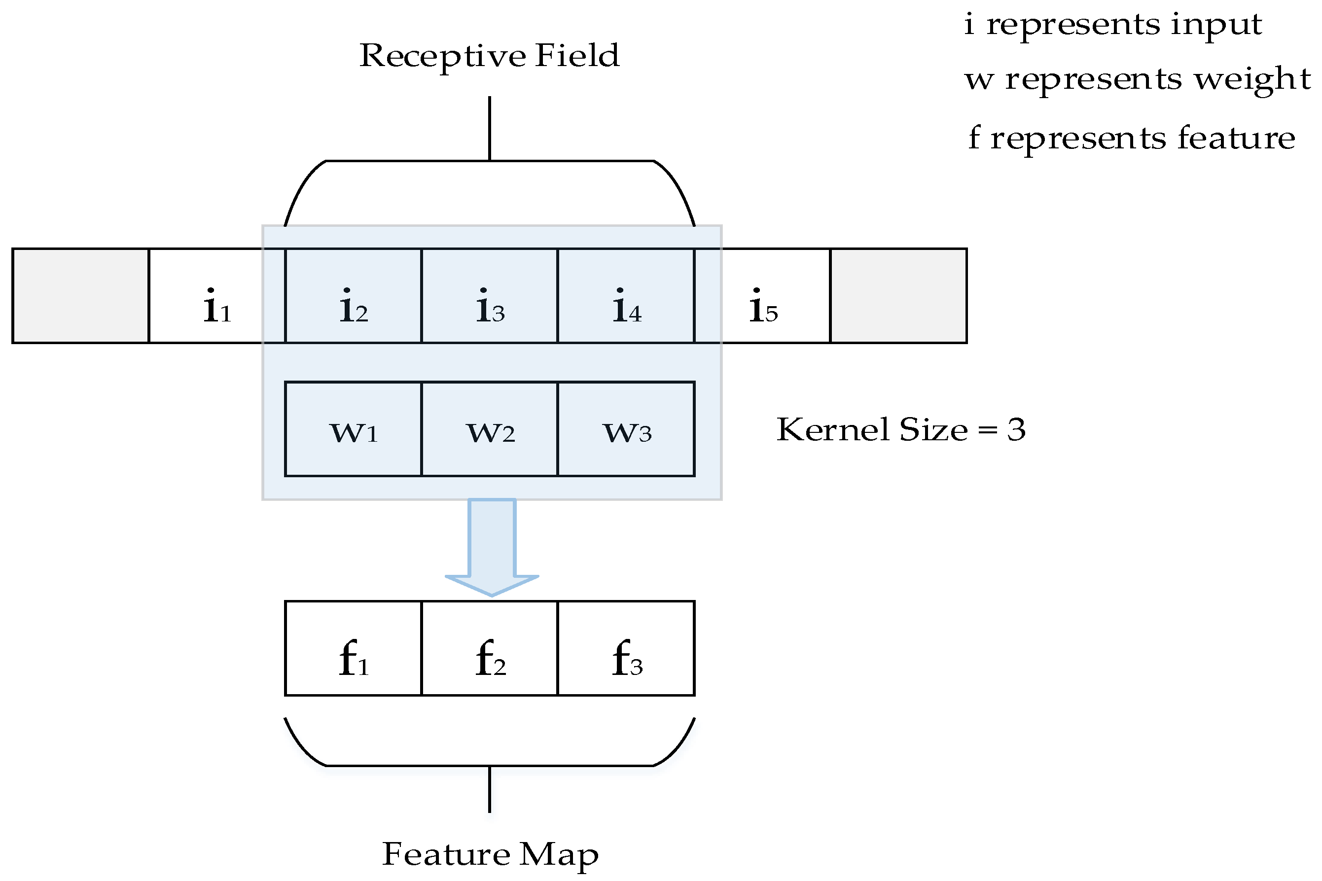
The convolutional layer is the most important building block of any CNN. This layer is regarded as a set of learnable filters that consists of many convolution operations. The parameters of every convolution operation are optimized by a back propagation algorithm. Each filter in a specific convolution layer has the same receptive field. An example of 1D convolution is shown in Figure 4. The weights associated with kernel size of 3 are {w1, w2, w3}. These weights are shared by the input layer {i1, i2, i3, i4, i5}. The feature map will be obtained by the convolution between the weights and inputs. In this example, the feature f2 is obtained by f2 = w1 × i2 + w2 × i3 + w3 × i4.
3.1.2. ReLU
The activation functions are used to enhance the ability of models to learn complex structures. ReLU has been widely adopted by various researchers to make the network more trainable. It works by thresholding values at 0, i.e., f (z) = max (0, z).
3.1.3. Dropout
The dropout technology provides an easy way to overcome the overfitting problem while designing the deep learning model. This method involves the random selection of neurons and disabling them during training. The output values of these randomly disabled neurons are zero.
3.1.4. Fully-Connected Layer
The fully connected layer exhibits the nonlinear mapping from the input to the output, by using bias and an activation function. These layers are usually applied towards the end of the network. We use the flatten layer after the convolution layers, as this layer expects 1-D data.
3.2. Proposed Model
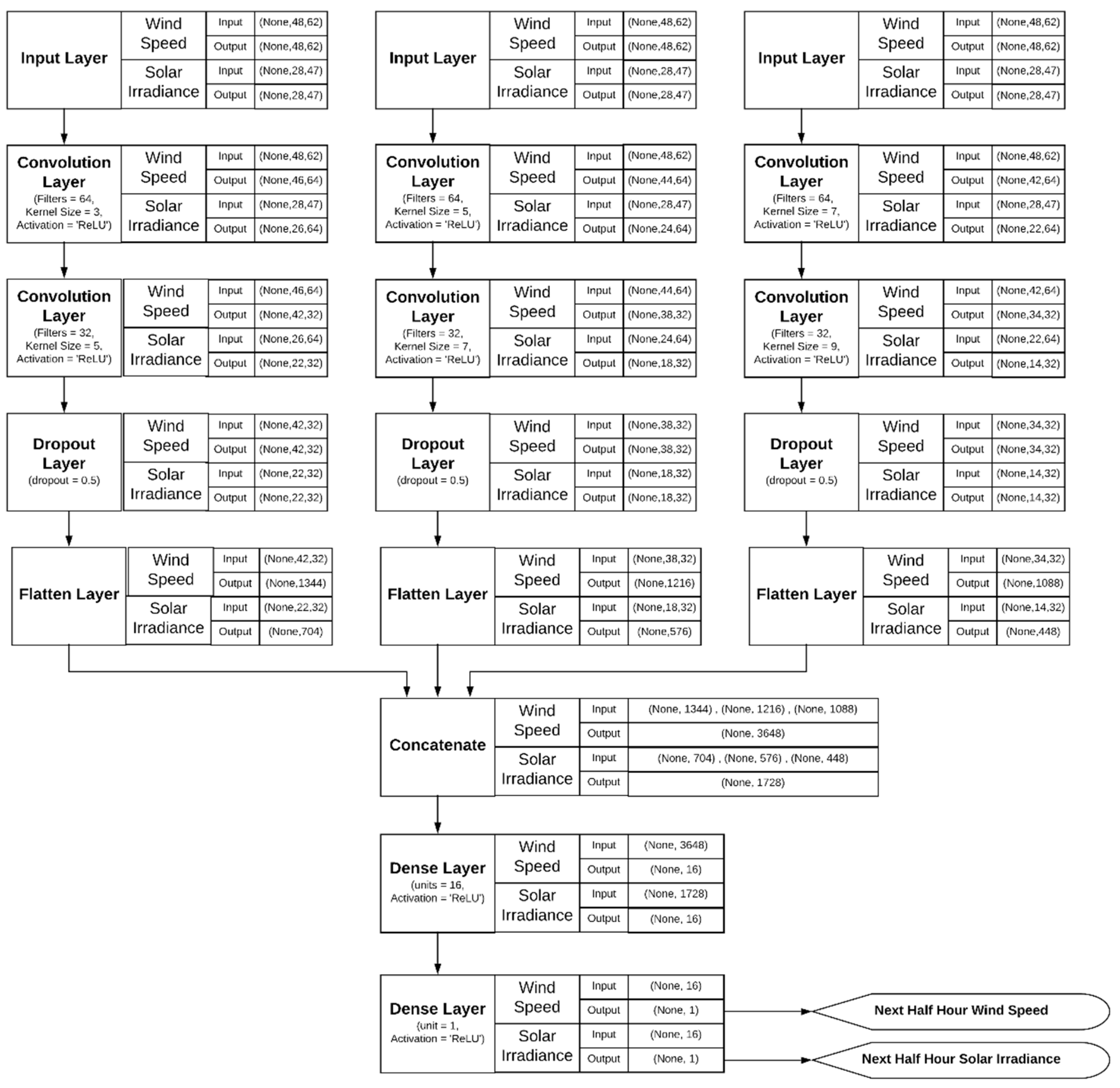
The details of our proposed MH-CNN model are shown in Figure 5. The number of features for wind speed and solar irradiance short-term forecasting are 62 and 47, respectively. For wind speed forecasting, there are 48 instances per day, as the data are recorded every 30 min. However, for solar irradiance forecasting, we considered the data from 5:30 to 19:00; hence, there are 28 instances per day. We used 64 filters in the first convolution layer with kernel sizes of 3, 5, and 7 for each head of the MH-CNN. Similarly, we used 32 filters in the second convolution layer with kernel sizes of 5, 7, and 9. We used a dropout value of 0.5 before applying the flattening layer. After concatenating all of the features into a single feature vector, a fully connected layer was applied with 16 neurons and the ReLU as a nonlinear activation function. The parameter settings of the proposed model are listed in Table 2. The prediction of both wind speed and solar irradiance concerns half-hour-ahead prognosis. The proposed model forecasts the next half hour value using the values of the previous day as inputs.
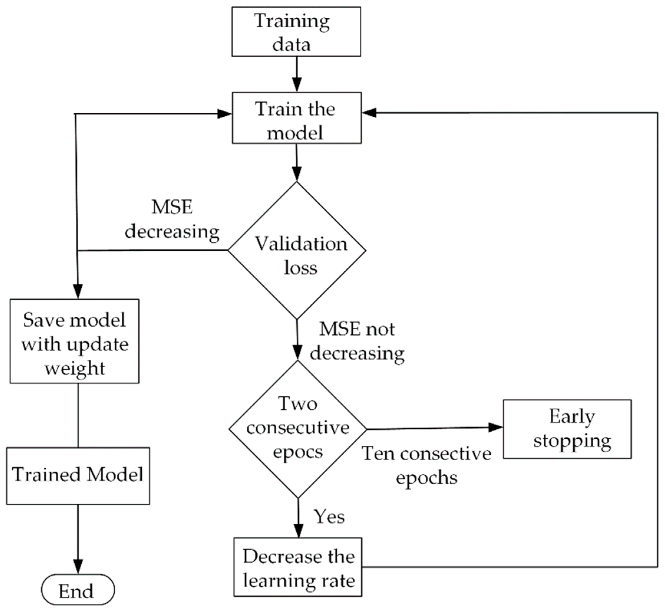
The training flow of the proposed model is shown in Figure 6. The training data are split into 90% training data and 10% validation data. The validation loss is based on the Mean Square Error (MSE) value. If the validation loss does not decrease for two consecutive epochs, then the learning rate is reduced by a factor of 0.85. The minimum value of the learning rate is set to be 1 × 10⁻⁶. If the validation loss is decreasing, then the model is saved with the updated weights. To avoid overfitting of the model during the training process, if the validation loss is not decreasing for 10 consecutive epochs, then early stopping callback is applied, and the last-saved best model is loaded for forecasting and performance evaluation. Otherwise, the training process continues until the maximal number of epochs is completed.
The performance of the trained model is evaluated based on various metrics, including RMSE, MAE, and MBE. The mathematical calculation methods of these performance matrices with their equations are shown in Equations (1) to (3).
where am is the actual value, and pm is the predicted value. The RMSE, MAE, and MBE represents model prediction error in units of the target variable. The RMSE gives a relatively high weightage to the outliers compared to MAE, as the residual is squared before averaging. The MAE is a linear score where all the individual differences are weighted equally. The MBE indicates the degree to which the observations are “over” or “under” forecasted by the prediction model. The smaller RMSE, MAE, and MBE denote the good performance of a forecasting model. MAPE is another standard metric for evaluating the performance of forecasting algorithms. Problems in its use can occur when am is zero or very small. As an alternative, we used sMAPE, as shown in Equation (4):
4. Performance Evaluation of Proposed Model
In this study, weather data from 1998 to 2007 for San Francisco, California, are used. The data were retrieved from the NSRDB of the NREL [67]. The first nine years of data are used to train the model, and the data for the last year (2007) are used to test the performance of the trained model.
4.1. Short-Term Forecasting Analysis of Wind Speed
We selected KNN, gradient boosting, extra tree regressor, and random forest regressor as our machine learning models. The input to all these models is the complete set of features mentioned in Figure 3. We used the default values of the parameters for our baseline model comparison. We used MSE as the loss function for all machine learning models in this study.
We also considered the persistence model for the short-term forecasting of wind speed. The persistence model assumes that wind data at a certain future time (the next half hour, in our case) will be the same as when the forecast was made. In this study, for the persistence model, we assumed that the wind data in the next half hour will be the same as that of the current time.
For our baseline model comparison, the parameters of various machine learning algorithms are taken from a previous study [8] and shown in Table 3.
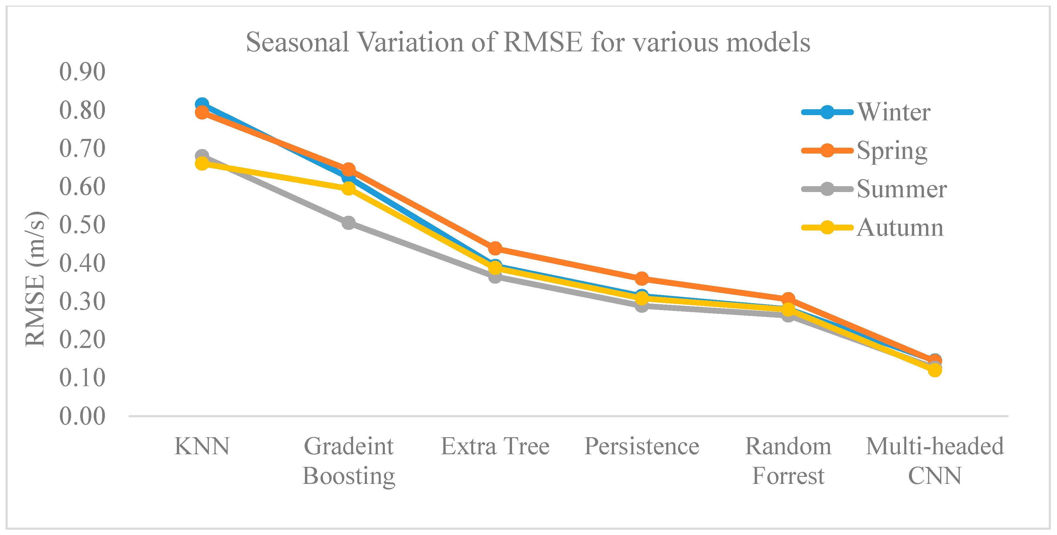
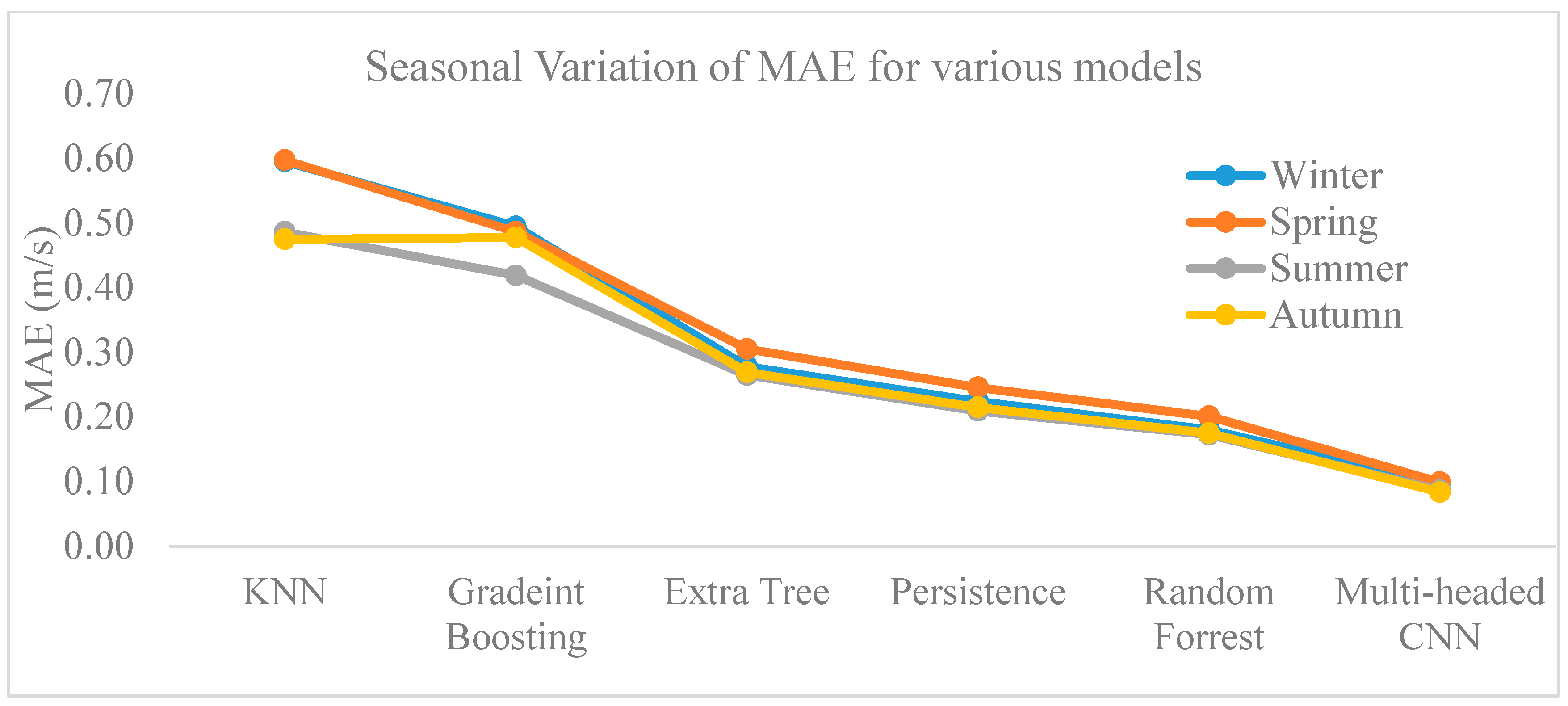
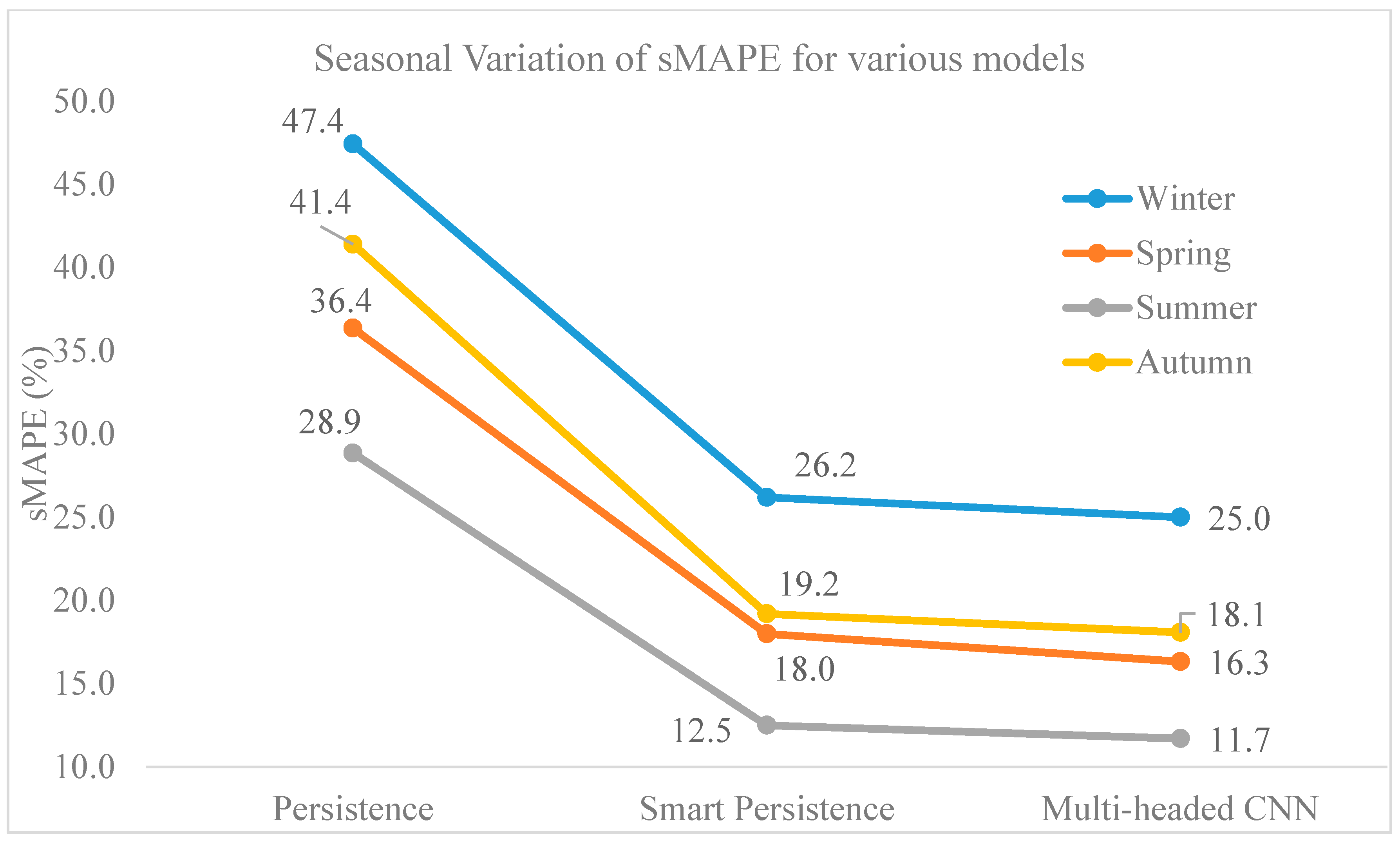
All trained machine learning models were evaluated on the same test data. We selected three standard evaluation metrics for comparing the performance of these models: RMSE, MAE, and sMAPE. Based on the test data set of one year, i.e., 2007, the seasonal average values (three-months-average values of RMSE, MAE, and sMAPE, with spring season defined as March, April, and May) are calculated. The seasonal variation of RMSE, MAE, and sMAPE are shown in Figure 7, Figure 8 and Figure 9, respectively. It is clear from these figures that the random forest method outperforms the persistence model, and therefore serves as the baseline model. The RMSE, MAE, and sMAPE of our proposed model are the lowest among the evaluated models.
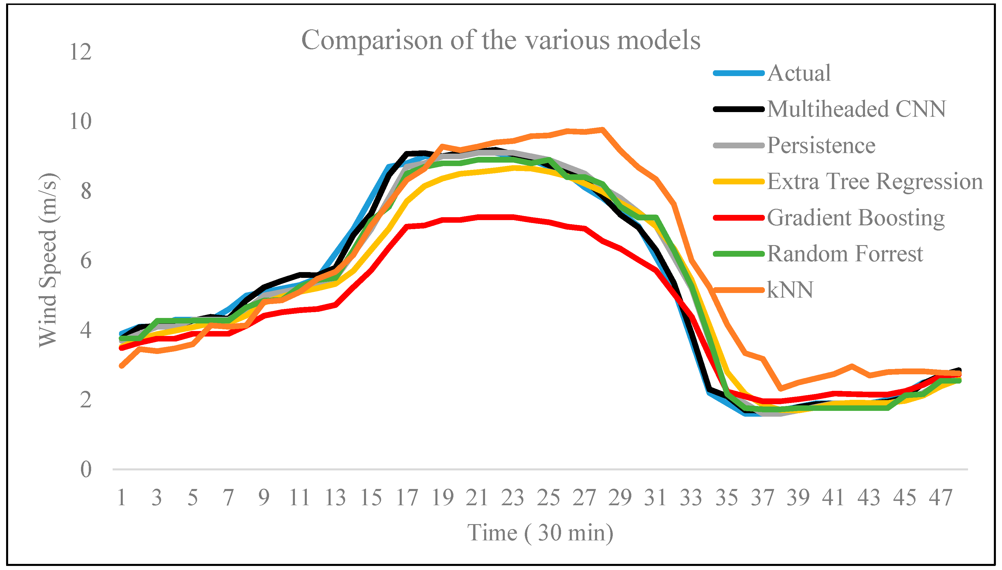
We have selected a random day from the test data to demonstrate the comparison of various machine learning models with the proposed model. Detailed comparison results of the wind speed prediction for all of the evaluated models are presented in Figure 10. The bold blue line represents the actual wind speed, whereas the bold black line represents the forecast by the proposed model. A careful analysis of this figure reveals that the forecast results of the KNN and gradient boosting algorithms barely coincide with the actual wind speed. The wind speed predicted by our proposed model is quite close to the actual wind speed. The forecasting ability of the proposed model is also verified in this experiment. The independent axis in this figure shows 48 values because of the 30 min sampling interval of the measured data.
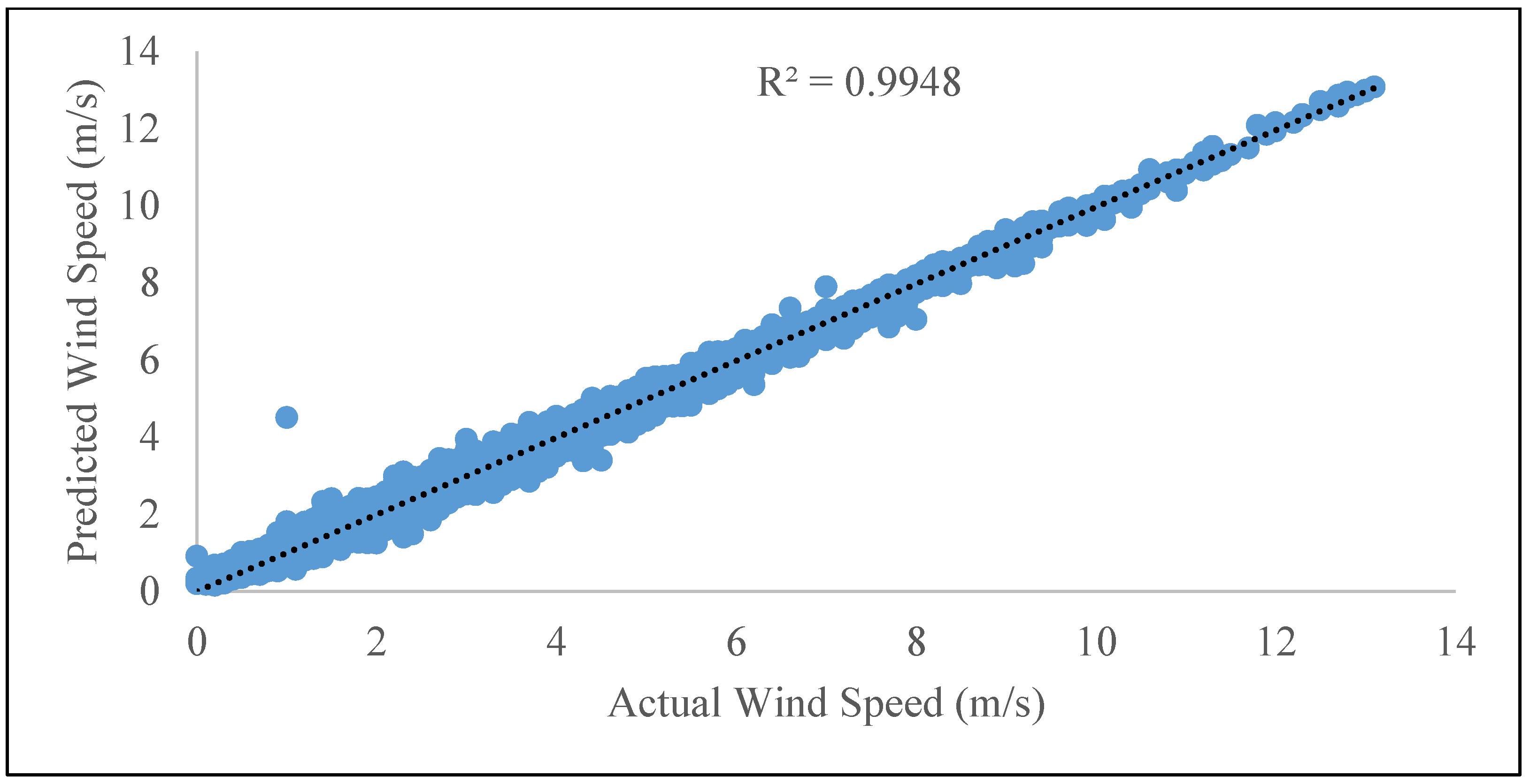
In Figure 11, a scatter plot of the predicted and actual wind speed values for the complete test data is presented. The coefficient of determination value is 0.9948, which confirms the strong, positive, linear association between the predicted and actual wind speeds. Furthermore, the coefficient of determination shows that the proposed model is able to explain 99.48% of the variation of the actual data. This indicates the very good forecasting ability of the proposed model.
Previous results (Figure 7, Figure 8 and Figure 9) showed the evaluation performance of various models for seasonal trends. Furthermore, we evaluated the performance of the selected models on the complete test data. These results are listed in Table 4 and Table 5.
Table 4 shows a comparison of the various models on the basis of the evaluation metrics for the selection of a baseline model. The results indicate that the KNN and gradient boosting algorithms perform poorly on the complete test data. Usually, it is difficult to outperform the persistence model for short-term forecasting. We can see that the random forest method outperformed the persistence model. Therefore, we selected random forest as a baseline model for comparison with our proposed model.
The comparison of our proposed model with the baseline model is presented in Table 5. It is clear from this table that the proposed MH-CNN model resulted in much lower (better) evaluation metrics than the baseline model. The percentages of error reductions achieved by the proposed model for RMSE, MAE, and sMAPE are 44.94, 46.12, and 2.25, respectively.
4.2. Short-Term Forecasting Analysis of Solar Irradiance
In solar irradiance forecasting, the persistence model usually serves as a baseline model for short-term forecasting. A simple persistence model [36] is shown in Equation (5):
where GHI(t) is the current global horizontal irradiance (GHI) at the surface. (The terms “solar irradiance” and “GHI” are used interchangeably throughout the manuscript.)
We selected another model with which to compare our proposed model: a variant of the persistence model, called the smart persistence model [36]. It is defined as
where kt(t) is the clear-sky index correction factor, defined as
Based on the test data of solar irradiance for the year 2007, Figure 12 and Figure 13 show the seasonal average variations for the persistence, smart persistence, and proposed models in terms of RMSE and sMAPE, respectively. It is clear from these figures that RMSE and sMAPE of our proposed model are lower than those of the persistence and smart persistence models. This shows that our proposed model is suitable for the short-term forecasting of solar irradiance.
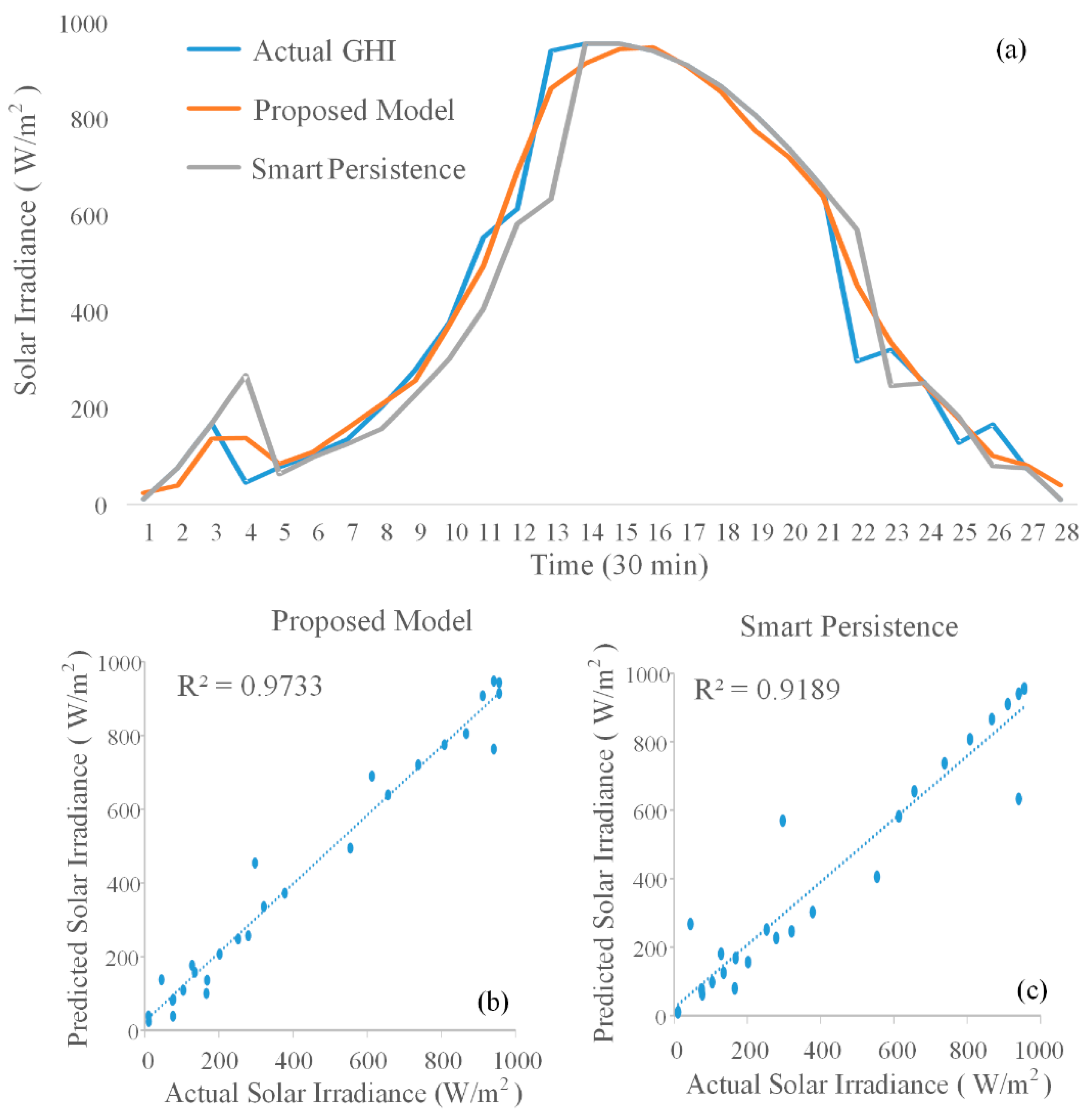
A comparison of the actual GHI and predicted solar irradiance using the proposed model and the smart persistence model is shown in Figure 14a. We selected a random day from the test data to demonstrate the comparison of the smart persistence model with the proposed model. The prediction accuracies of the proposed model and smart persistent model are shown in Figure 14b and Figure 14c, respectively. The coefficient of determination of the proposed model is reasonably high compared to that of the smart persistence model, which shows that our proposed model can be successfully applied to predict the solar irradiance. Later, we used the predicted solar irradiance to approximate the generated solar energy.
A comparison of the persistence and smart persistence models for the selection of the best model is presented in Table 6. As seen from the results, the smart persistence model is best as a baseline model for comparison with the proposed model.
A comparison of the proposed model with the smart persistence model is presented in Table 7. It is clear from the results of this table that the proposed model produced better results than the smart persistence model. We achieved 7.68%, 54.29%, and 0.14% error reductions in the RMSE, MBE, and sMAPE, respectively.
5. Results and Discussions
In this section, we evaluated the effectiveness of the proposed model for different forecasting horizons and different climates. Then, we performed a comprehensive bill reduction analysis by estimating the generated power from renewable resources using the data of San Francisco as a case study.
5.1. Evaluation of Proposed Model for Different Time Horizons
In the previous section, we explored the effectiveness of the proposed model for a single-step forecast, i.e., predicting the observation at the next time stamp. To illustrate the effectiveness of the proposed model for multi-step forecasting, i.e., different time horizons, we considered the same data used in Section 4. The output of the proposed model was reshaped according to the forecasting time horizon. For example, when the time horizon was set to 4 h ahead, then the model was evaluated such that for each instance of test data, the model will predict the next eight values in one-shot.
Table 8 shows the seasonal RMSE variation of the proposed model for wind speed and solar irradiance forecasting of different time horizons.
5.2. Evaluation of Proposed Model for Different Climates
In Section 4, we tested the proposed model on San Francisco (Latitude: 37.77, Longitude: −122.42), which has a warm summer Mediterranean climate. In order to demonstrate the effectiveness of the proposed model in a different climate, we selected New York (Latitude: 40.73, Longitude: −74.02), which has a humid subtropical climate, and Las Vegas (Latitude: 33.61, Longitude: −114.58), which has a hot desert climate. In this experiment, data from 1998 to 2007 for New York and Las Vegas is used. The data were retrieved from the NSRDB of the NREL [67]. We prepared the training and test data according to Figure 3 for both sites. The first nine years of data (1998–2006) was used to train the model and the last one year of data (2007) was used to test the performance of the trained model.
To fairly compare the RMSE across different sites, normalized root mean square error (nRMSE) is computed as,
where is the mean of the actual values. Table 9 shows the seasonal variation of the proposed model for short-term forecasting of wind speed and solar irradiance for different climates.
As seen in the table, for each season, there is a small discrepancy between the wind speed nRMSE of various sites with different climates. This result indicates that our proposed model is capable of forecasting the short-term wind speed for different climates during various seasons with high accuracy.
For short-term forecasting of solar irradiance, there is an almost 9% difference between the best predictor (summer season) for San Francisco and New York. This discrepancy is certainly due to the cloud formation processes, which are very different in these two sites. The two sites experience different sky conditions during the year. Sites such as San Francisco and Las Vegas exhibit stable sky conditions during the summer. However, New York witnesses occasional thunderstorms with heavy rain in summer, and tornadoes are not uncommon.
There is an almost 5.6% difference between the worst predictor (winter season) of San Francisco and New York. In San Francisco and New York, the sky is mostly cloudy, around 55% and 53% of the time in winter, respectively. The proposed model performance is worst in winter, since the sky coverage is highly variable. In Las Vegas, there is a significant seasonal variation in the cloud coverage over the course of the year. For a hot desert climate, such as Las Vegas, the seasonal performance of the model is reasonably suitable for solar irradiance forecasting.
The result of the solar irradiance forecast indicates that the proposed model is well-suited for a hot desert climate, as well as a Mediterranean climate. Moreover, it can also be used for a humid subtropical climate.
5.3. Generation Estimation and Bill Reduction Analysis: San Francisco as a Case Study
We considered a smart community consisting of 80 homes as the consumers of the electricity. For simulation purposes, it was assumed that the smart community has a microgrid that is equipped with wind turbines and solar panels, in addition to having access to the power from the main grid. At any time, the energy generated by the wind turbine and solar panels is provided to the users through the microgrid, and the excess generated energy is stored in the ESS for later use. In addition, the deficit energy at any time is purchased from the commercial grid to satisfy the energy demands of the users in the smart community.
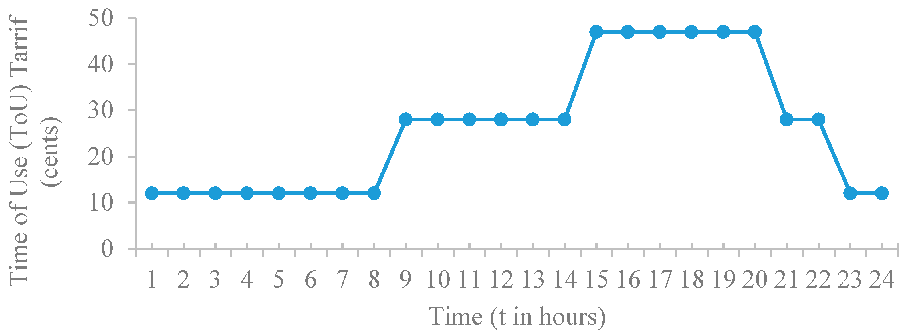
In this work, a Time of Use (ToU) pricing model is applied to determine the price of the consumed electricity [68], which is shown in Figure 15. A 24-h time period is considered and is denoted by T. This is divided into 1-h subintervals indicated by t.
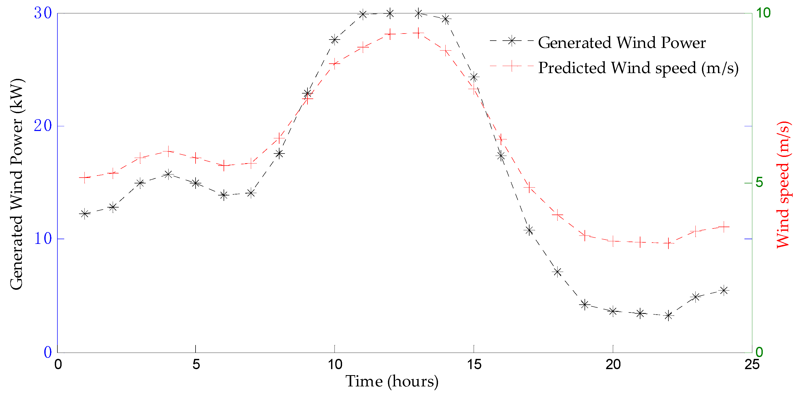
For a randomly selected day, the proposed model is applied to predict the wind speed for 24 h. The predicted wind speed is then used to approximate the generated wind energy based on Equation (8), which we also used in our recent work [69]. The predicted wind speed and generated wind power are presented in Figure 16. It is clear from the figure that with an increase in the wind speed, the power generated by the wind turbine also increases. The power generation of the wind turbine is approximated by implementing Equation (8) in MATLAB. For simulation purposes, we used a single wind turbine of 30 kW [70]. As shown in the figure, when the wind speed is equal to, or greater than, the rated wind speed of the selected wind turbine, the output power is the maximum attainable, which is the rated maximum power.
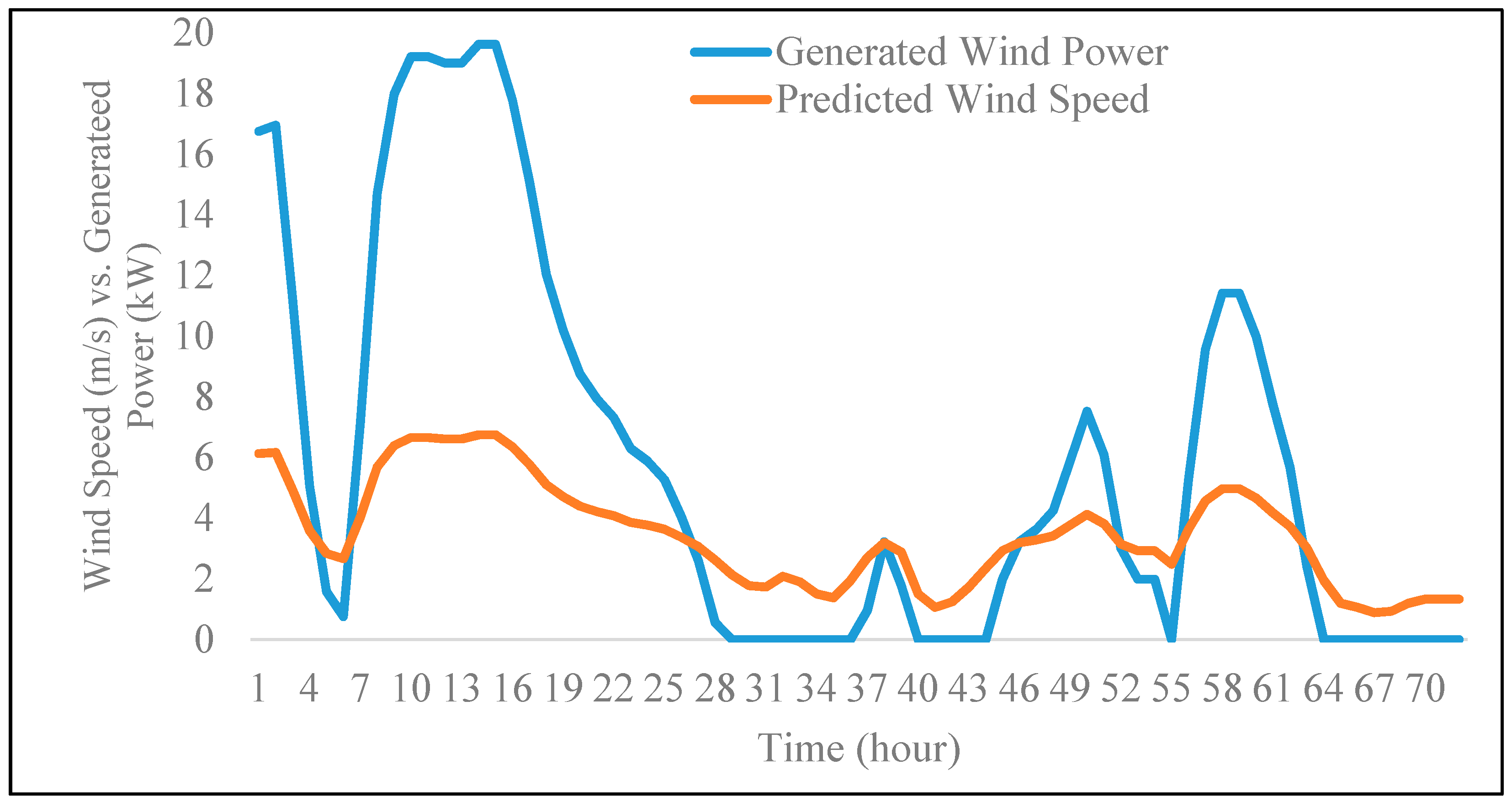
The predicted half-hour wind speed for three days and the associated generated wind power are shown in Figure 17. The fluctuations in the predicted wind speed at different times during the 72-h period are evident from the figure. As shown, when the wind speed is lower than the cut-in speed of the wind turbine, the generated power is zero.
In Equation (9), the power generated by the wind turbine is represented by Ptwt, and Cp is the power coefficient. It also depends on air density ρ, area swept by rotor blades A, and wind speed Vtwt. The wind turbine triggers are based on the cut-in and cut-out speeds. The association between the output power and the wind speed of the wind turbine is based on Equation (10) from a previous study [71]. In Equation (10), Pout is the output power, PR is the rated power, Vtwt is the wind speed at time t, Vci is the cut-in wind speed, and Vco is the cut-out wind speed. The technical specifications of the selected wind turbine are shown in Table 10.
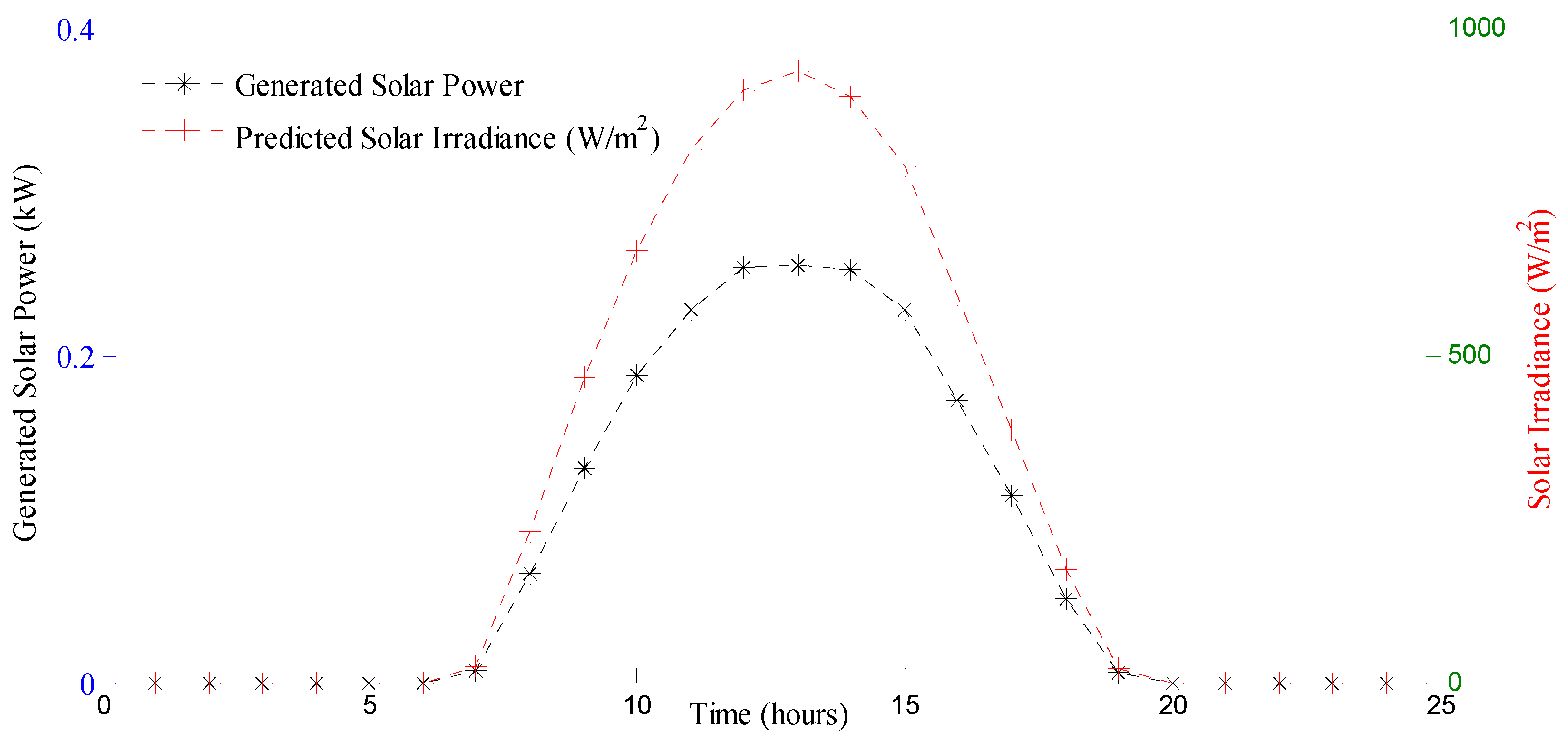
Figure 18 reveals the association between the power generated by the solar panel and the solar irradiance. We can observe that with an increase in the solar irradiance, the power generated by the solar panel also increases. The solar panel temperature data are taken from a previous study [72]. The solar irradiance is predicted using our proposed model. The power generation by the solar panel is approximated by implementing Equation (11) from our previous work [69] in MATLAB.
In Equation (11), the hourly generated power from the solar panel is represented by PtPV. The area and efficiency of the solar panel are represented by APV and ηPV, respectively. The solar irradiance is represented by Irr, and the hourly temperature of the solar panel is represented by Tt. In our simulations, we considered two solar panels per house, each at 300 W.
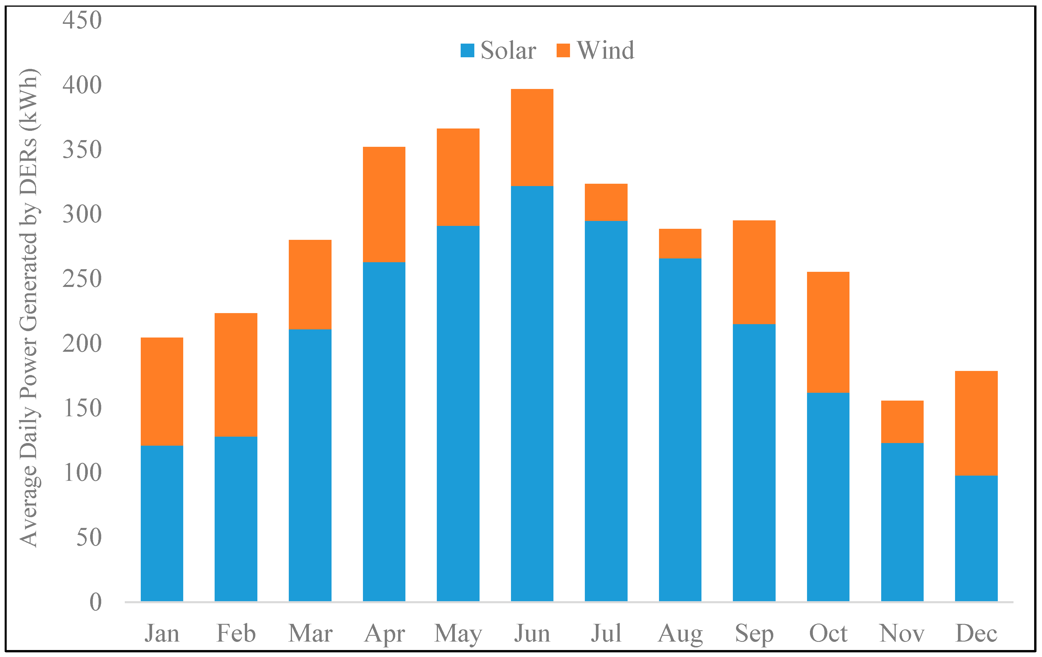
The proportions of the average daily power generated by the wind turbine and solar panels in each month of the year 2007 are presented in Figure 19. It is evident from the figure that the power generated by the solar panels varies predictably across the seasons, as expected. The month of June has the highest recorded average daily power generation using solar panels. The average daily power generated by the wind turbine is lowest in August and saw its best month in February.
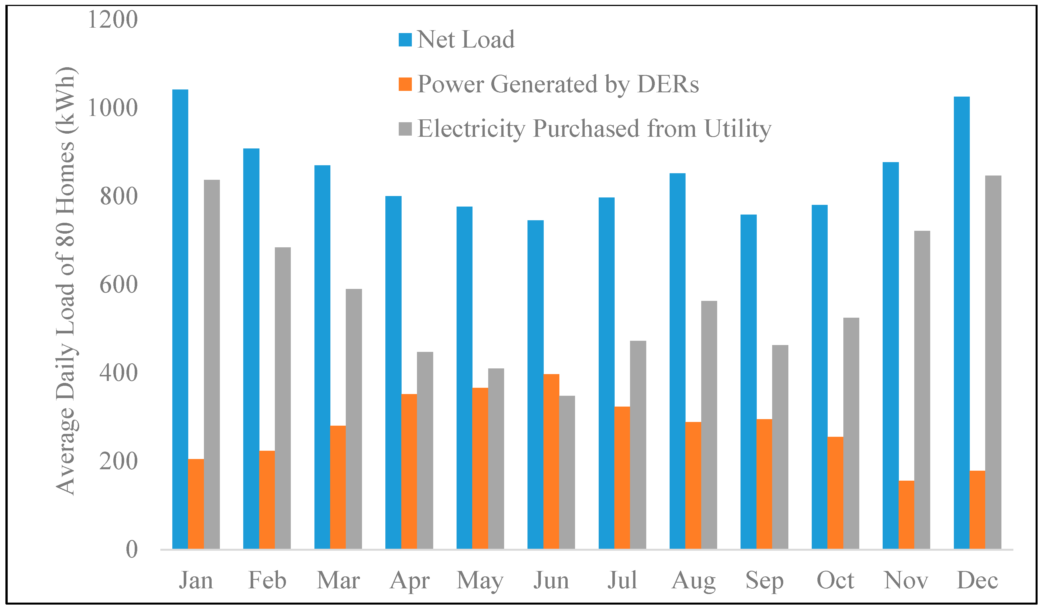
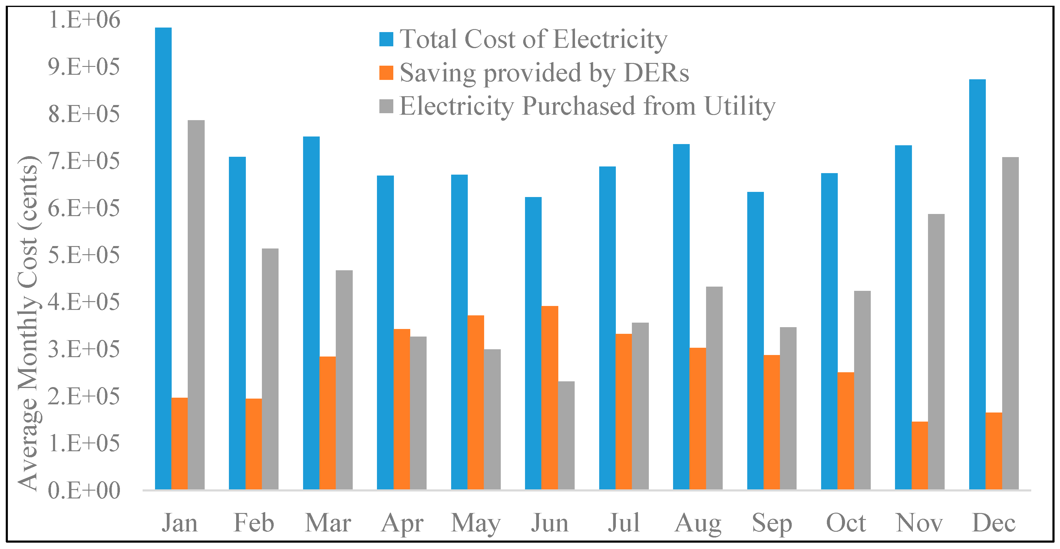
The net power load, power generated by DERs, and electricity purchased from the utility are shown in Figure 20. We took the average monthly electricity usage (net load) of households in San Francisco, California, from a previous study [73]. In this figure, we can observe that the total power generated by DERs is high during the months of May and June. This resulted in lower electricity costs when purchased from the utility. Various components of the average monthly cost of electricity for 80 homes are shown in Figure 21. As shown in the figure, savings are at a maximum in the month of June and at a minimum in the month of January.
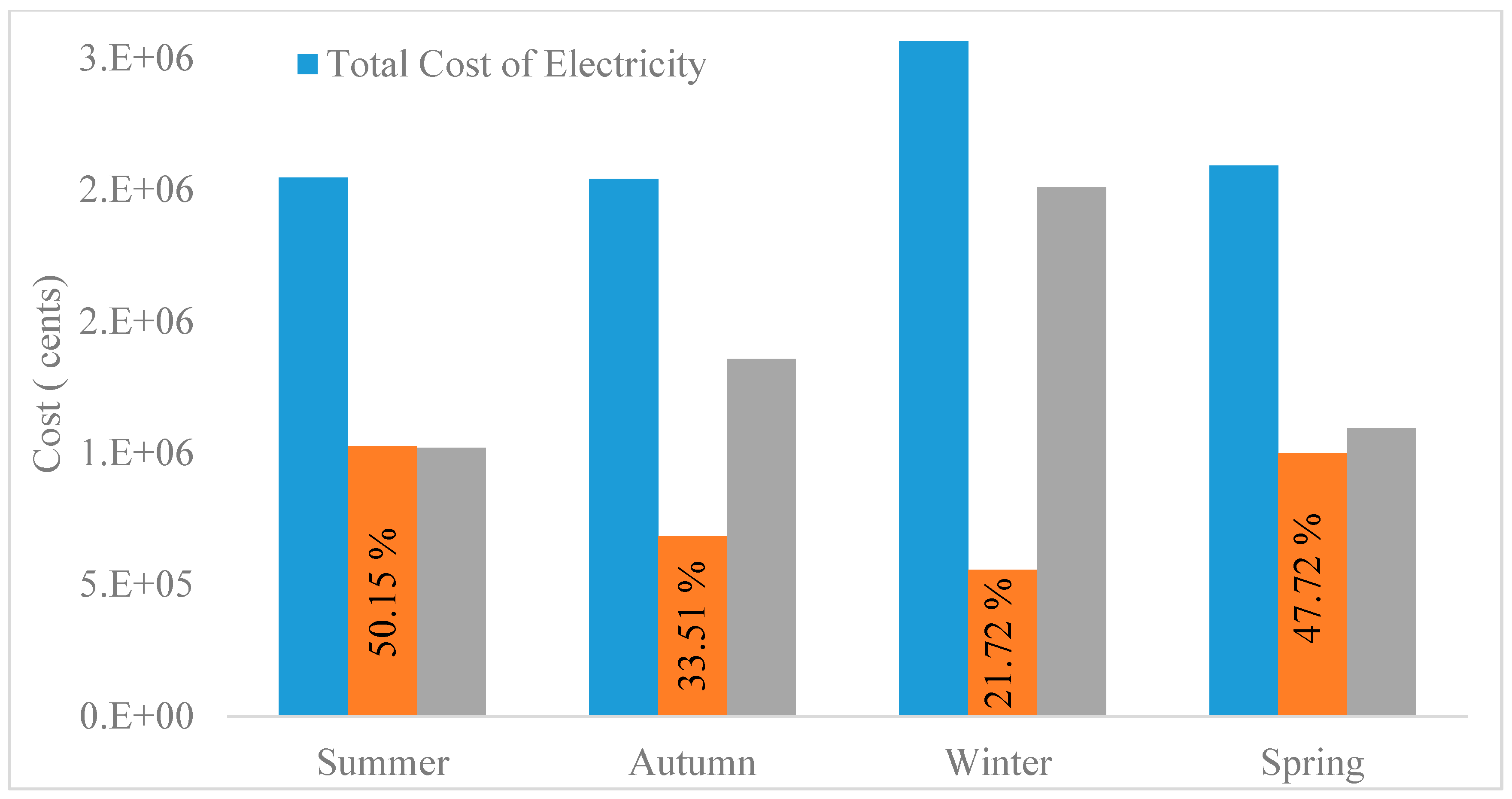
It can be observed from Figure 22 that the contribution of DERs during the winter season is not very significant. However, in the remaining seasons, significant relief is provided by the DERs in terms of bill reduction. Based on the numerical calculations of the bar graphs in Figure 22, it can be concluded that the proposed framework will help the smart community to achieve an annual reduction of up to 38% in their electricity bills by installing DERs.
6. Conclusions
DERs are valuable in decreasing consumers’ electricity bills by enabling them to generate their own green energy. However, the intermittent nature of DERs is a significant issue in accurately forecasting the amount of generated energy through these renewable energy resources. In this work, we proposed and evaluated an efficient approach to energy management in a smart community based on the integration of DERs. Sometimes, the energy generated through DERs is greater than the energy demand of the consumers, which results in a demand and generation mismatch.
The demand and generation mismatch leads to the well-known “duck curve” problem. We applied a machine learning model to accurately predict the generated energy through DERs. We considered a smart community consisting of 80 smart homes. The smart community has access to electric power through a microgrid that is equipped with DERs in the form of wind turbines and photovoltaic systems, in addition to having access to power from the main grid.
The simulation results indicated that our proposed framework is appropriate for approximating the energy generated through DERs and for reducing the electricity bills of the smart community. We evaluated the performance of several machine learning models for selecting a baseline model. Then, we evaluated the performance of our proposed model and compared it with the baseline model.
For the case of wind speed prediction, we obtained 44.94%, 46.12%, and 2.25% error reductions in the evaluation metrics of RMSE, MAE, and sMAPE, respectively. In the case of solar irradiance prediction, we obtained 7.6%, 54.3%, and 0.14% error reductions in the evaluation metrics of RMSE, MBE, and sMAPE, respectively.
We further evaluated the effectiveness of the proposed model in different climates and for different time horizons. The results conclude that the proposed model is not only suitable for short-term forecasting of wind speed and solar irradiance for different time horizons (up to four hours) but for different climates as well.
Author Contributions
Conceptualization, M.A., S.I.H. and K.A.; Methodology, M.A., S.I.H. and K.A.; Validation, S.I.H. and K.A.; Formal analysis, S.I.H. and K.A.; Investigation, M.A., S.I.H. and K.A.; Data curation, S.I.H. and K.A; Writing—original draft, K.A., M.A., and S.I.H.; Writing—review & editing, M.A., S.I.H. and K.A.; Project administration, M.A.; Funding acquisition, K.A.
Funding
The authors extend their appreciation to the Deanship of Scientific Research at King Saud University for funding this work through research group NO (RG-1438-034).
Conflicts of Interest
The authors declare no conflicts of interest.
References
- Commission Final Report: Integrated Energy Policy Report 2004 Update Publication #100-04-006CM. Available online: https://www.energy.ca.gov/2004_policy_update/ (accessed on 14 April 2019).
- Engeland, K.; Borga, M.; Creutin, J.-D.; François, B.; Ramos, M.-H.; Vidal, J.-P. Space-time variability of climate variables and intermittent renewable electricity production—A review. Renew. Sustain. Energy Rev. 2017, 79, 600–617. [Google Scholar] [CrossRef]
- Martin, L.; Zarzalejo, L.; Polo, J.; Navarro, A.; Marchante, R.; Cony, M. Prediction of global solar irradiance based on time series analysis: Application to solar thermal power plants energy production planning. Sol. Energy 2010, 84, 1772–1781. [Google Scholar] [CrossRef]
- Falayi, E.; Adepitan, J.; Rabiu, A. Empirical models for the correlation of global solar radiation with meteorological data for Iseyin, Nigeria. Phys. Sci. 2008, 3, 210–216. [Google Scholar]
- Paolik, C.; Voyant, C.; Muselli, M.; Nivet, M. Solar radiation forecasting using ad-hoc time series preprocessing and neural networks. In Proceedings of the 5th International Conference on Emerging Intelligent Computing Technology and Applications, Ulsan, Korea, 16–19 September 2009; pp. 898–907. [Google Scholar]
- Paulescu, M.; Paulescu, E.; Gravila, P.; Badescu, V. Modeling solar radiation at the earth surface. In Weather Modeling and Forecasting of PV Systems Operation; Springer: Berlin, Germany, 2012. [Google Scholar]
- Liu, L.; Liu, D.; Sun, Q.; Li, H.; Wennersten, R. Forecasting power output of photovoltaic system using a BP network method. Energy Procedia 2017, 142, 780–786. [Google Scholar] [CrossRef]
- Bouktif, S.; Fiaz, A.; Ouni, A.; Serhani, M.A. Optimal deep learning LSTM model for electric load forecasting using feature selection and genetic algorithm: Comparison with machine learning approaches. Energies 2018, 11, 1636. [Google Scholar] [CrossRef]
- Hossain, M.; Mekhilef, S.; Danesh, M.; Olatomiwa, L.; Shamshirband, S. Application of extreme learning machine for short term output power forecasting of three grid-connected PV systems. J. Clean. Prod. 2017, 167, 395–405. [Google Scholar] [CrossRef]
- Bendu, H.; Deepak, B.B.V.L.; Murugan, S. Multi-objective optimization of ethanol fuelled HCCI engine performance using hybrid GRNN–PSO. Appl. Energy 2017, 187, 601–611. [Google Scholar] [CrossRef]
- Deo, R.C.; Wen, X.; QiA, F. Wavelet-coupled support vector machine model for forecasting global incident solar radiation using limited meteorological dataset. Appl. Energy 2016, 168, 568–593. [Google Scholar] [CrossRef]
- Lin, S.; Liu, X.; Fang, J.; Xu, Z. Is extreme learning machine feasible? A theoretical assessment (Part II). IEEE Trans. Neural Netw. Learn. Syst. 2015, 26, 21–34. [Google Scholar] [CrossRef] [PubMed]
- Mareček, J. Usage of Generalized Regression Neural Networks in Determination of the Enterprise’s Future Sales Plan. Littera Scr. 2016, 3, 32–41. [Google Scholar]
- Bhavsar, H.; Panchal, M.H. A Review on Support Vector Machine for Data Classification. Int. J. Adv. Res. Comput. Eng. Technol. 2012, 1, 185–189. [Google Scholar]
- Shireen, T.; Shao, C.; Wang, H.; Li, J.; Zhang, X.; Li, M. Iterative multi-task learning for time-series modeling of solar panel PV outputs. Appl. Energy 2018, 21, 654–662. [Google Scholar] [CrossRef]
- Wang, F.; Zhen, Z.; Mi, Z.; Sun, H.; Su, S.; Yang, G. Solar irradiance feature extraction and support vector machines based weather status pattern recognition model for short-term photovoltaic power forecasting. Energy Build. 2015, 86, 427–438. [Google Scholar] [CrossRef]
- Ramsami, P.; Oree, V. A hybrid method for forecasting the energy output of photovoltaic systems. Energy Convers. Manag. 2015, 95, 406–413. [Google Scholar] [CrossRef]
- Xiea, J.; Lib, H.; Maa, Z.; Sunc, Q.; Wallinb, F.; Sid, Z.; Gu, J. Analysis of key factors in heat demand prediction with neural networks. Energy Procedia 2017, 105, 2965–2970. [Google Scholar] [CrossRef]
- Ma, Z.; Hue, J.H.; Leijon, A.; Tan, Z.H.; Yang, Z.; Guo, J. Decorrelation of neutral vector variables: Theory and applications. IEEE Trans. Neural Netw. 2016, 29, 129–143. [Google Scholar] [CrossRef]
- Cococcioni, M.; D’Andrea, E.; Lazzerini, B. Twenty-four-hour-ahead forecasting of energy production in solar PV systems. In Proceedings of the IEEE International Conference on Intelligent Systems Design and Applications, Cordoba, Spain, 22–24 November 2011; pp. 1276–1281. [Google Scholar]
- Chu, Y.; Urquhart, B.; Gohari, S.M.I.; Pedro, H.T.C.; Kleissl, J.; Coimbra, C.F.M. Short-term reforecasting of power output from a 48 MW solar PV plant. Sol. Energy 2015, 112, 68–77. [Google Scholar] [CrossRef]
- Hussain, S.; AlAlili, A. Hybrid solar radiation modelling approach using wavelet multiresolution analysis and artificial neural networks. Appl. Energy 2017, 208, 540–550. [Google Scholar] [CrossRef]
- Larraondo, P.R.; Inza, I.; Lozano, J.A. Automating weather forecasts based on convolutional networks. In Proceedings of the ICML Workshop on Deep Structured Prediction, PMLR 70, Sydney, Australia, 11 August 2017. [Google Scholar]
- Zhuang, W.Y.; Ding, W. Long-lead prediction of extreme precipitation cluster via a spatio-temporal convolutional neural network. In Proceedings of the 6th International Workshop on Climate Informatics: CI 2016, Boulder, CO, USA, 22–23 September 2016. [Google Scholar]
- Sulagna Gope, P.M.; Sarkar, S. Prediction of extreme rainfall using hybrid convolutional-long short term memory networks. In Proceedings of the 6th International Workshop on Climate Informatics, Boulder, CO, USA, 22–23 September 2016. [Google Scholar]
- Han, Q.; Wu, H.; Hu, T.; Chu, F. Short-term wind speed forecasting based on signal decomposing algorithm and hybrid linear/nonlinear models. Energies 2018, 11, 2976. [Google Scholar] [CrossRef]
- Rabanal, A.; Ulazia, A.; Ibarra-Berastegi, G.; Sáenz, J.; Elosegui, U. MIDAS: A Benchmarking Multi-Criteria Method for the Identification of Defective Anemometers in Wind Farms. Energies 2019, 12, 28. [Google Scholar] [CrossRef]
- Huang, C.-J.; Kuo, P.-H. A Short-Term Wind Speed Forecasting Model by Using Artificial Neural Networks with Stochastic Optimization for Renewable Energy Systems. Energies 2018, 11, 2777. [Google Scholar] [CrossRef]
- Ssekulima, E.B.; Anwar, M.B.; Al Hinai, A.; El Moursi, M.S. Wind speed and solar irradiance forecasting techniques for enhanced renewable energy integration with the grid: A review. IET Renew. Power Gener. 2016, 7, 885–989. [Google Scholar] [CrossRef]
- Yahyaoui, I. Forecasting of Intermittent Solar Energy Resource, Advances in Renewable Energies and Power Technologies, 1st ed.; Volume 1: Solar and Wind Energies; Elsevier Science: Amsterdam, The Netherlands, 2018; Chapter 3; pp. 78–114. [Google Scholar]
- Coimbra Carlos, F.M.; Kleissl, J.; Marquez, R. Overview of Solar-Forecasting Methods and a Metric for Accuracy Evaluation. In Solar Energy Forecasting and Resource Assessment; Elsevier Academic Press: Amsterdam, The Netherlands, 2013; Chapter 8; pp. 171–194. [Google Scholar]
- Zhang, J.; Florita, A.; Hodge, B.-M.; Lu, S.; Hamann, H.F.; Banunarayanan, V.; Brockway, A.M. A suite of metrics for assessing the performance of solar power forecasting. Sol. Energy 2015, 111, 157–175. [Google Scholar] [CrossRef] [Green Version]
- Tuohy, A.; Zack, J.; Haupt, S.E.; Sharp, J.; Ahlstrom, M.; Dise, S.; Grimit, E.; Mohrlen, C.; Lange, M.; Casado, M.G.; et al. Solar Forecasting: Methods, Challenges, and Performance. IEEE Power Energy Mag. 2015, 13, 50–59. [Google Scholar] [CrossRef]
- Reikard, G.; Hansen, C. Forecasting solar irradiance at short horizons: Frequency and time domain models. Renew. Energy 2019, 135, 1270–1290. [Google Scholar] [CrossRef]
- Kleissl, J. Current State of the Art in Solar Forecasting; Technical Report; California Institute for Energy and Environment: Berkeley, CA, USA, 2010. [Google Scholar]
- Kumler, A.; Xie, Y.; Zhang, Y. A New Approach for Short-Term Solar Radiation Forecasting Using the Estimation of Cloud Fraction and Cloud Albedo; NREL/TP-5D00-72290; National Renewable Energy Laboratory (NREL): Golden, CO, USA, 2018.
- Pedro Hugo, T.C.; Coimbra Carlos, F.M.; David, M.; Lauret, P. Assessment of machine learning techniques for deterministic and probabilistic intra-hour solar forecasts. Renew. Energy 2018, 123, 191–203. [Google Scholar] [CrossRef]
- Ma, J.; Makarov, Y.V.; Loutan, C.; Xie, Z. Impact of wind and solar generation on the California ISO’s intra-hour balancing needs. In Proceedings of the 2011 IEEE Power and Energy Society General Meeting, San Diego, CA, USA, 24–29 July 2011. [Google Scholar]
- Huang, R.; Huang, T.; Gadh, R. Solar Generation Prediction using the ARMA Model in a Laboratory-level Micro-grid. In Proceedings of the 2012 IEEE Third International Conference on Smart Grid Communications, Tainan, Taiwan, 5–8 November 2012; pp. 528–533. [Google Scholar]
- Bouzgou, H.; Gueymard, C.A. Fast short-term global solar irradiance forecasting with wrapper mutual information. Renew. Energy 2019, 133, 1055–1065. [Google Scholar] [CrossRef]
- Benali, L.; Notton, G.; Fouilloy, A.; Voyant, C.; Dizene, R. Solar radiation forecasting using artificial neural network and random forest methods: Application to normal beam, horizontal diffuse and global components. Renew. Energy 2019, 132, 871–884. [Google Scholar] [CrossRef]
- Crisosto, C.; Hofmann, M.; Mubarak, R.; Seckmeyer, G. One-Hour Prediction of the Global Solar Irradiance from All-Sky Images Using Artificial Neural Networks. Energies 2018, 11, 2906. [Google Scholar] [CrossRef]
- Lago, J.; De Brabandere, K.; De Ridder, F.; De Schutter, B. Short-term forecasting of solar irradiance without local telemetry: A generalized model using satellite data. Sol. Energy 2018, 173, 566–577. [Google Scholar] [CrossRef]
- Jadidi, A.; Menezes, R.; De Souza, N.; Lima, A.C.D. A Hybrid GA-MLPNN Model for One-Hour-Ahead Forecasting of the Global Horizontal Irradiance in Elizabeth City, North Carolina. Energies 2018, 11, 2641. [Google Scholar] [CrossRef]
- Alfadda, A.; Rahman, S.; Pipattanasomporn, M. Solar irradiance forecast using aerosols measurements: A data driven approach. Sol. Energy 2018, 170, 924–939. [Google Scholar] [CrossRef]
- California Energy Commission Report: Toward a Clean Energy Future. Publication # CEC-100-2018-001-V1. Available online: https://www.energy.ca.gov/2018publications/CEC-100-2018-001/. (accessed on 14 April 2019).
- NSRD from NREL. Available online: https://nsrdb.nrel.gov/current-version (accessed on 10 March 2019).
- Sengupta, M.; Xie, Y.; Lopez, A.; Habte, A.; Maclaurin, G.; Shelby, J. The National Solar Radiation Data Base (NSRDB). Renew. Sustain. Energy Rev. 2018, 89, 51–60. [Google Scholar] [CrossRef]
- Aslam, S.; Iqbal, Z.; Javaid, N.; Khan, Z.A.; Aurangzeb, K.; Haider, S.I. Towards efficient energy management of smart buildings exploiting heuristic optimization with real time and critical peak pricing schemes. Energies 2017, 12, 2065. [Google Scholar] [CrossRef]
- Mohsenian-Rad, A.-H.; Wong, V.W.S.; Jatskevich, J.; Schober, R.; Leon-Garcia, A. Autonomous demand-side management based on game-theoretic energy consumption scheduling for the future smart grid. IEEE Trans. Smart Grid 2010, 1, 320–331. [Google Scholar] [CrossRef]
- Niyato, D.; Xiao, L.; Wang, P. Machine-to-machine communications for home energy management system in smart grid. IEEE Commun. Mag. 2011, 49, 53–59. [Google Scholar] [CrossRef]
- Lidula, N.; Rajapakse, A.D. Microgrids research: A review of experimental microgrids and test systems. Renew. Sustain. Energy Rev. 2011, 15, 186–202. [Google Scholar] [CrossRef]
- Mehrizi-Sani, A.; Iravani, R. Potential-function based control of a microgrid in islanded and grid-connected modes. IEEE Trans. Power Syst. 2010, 25, 1883–1891. [Google Scholar] [CrossRef]
- Farhangi, H. The path of the smart grid. IEEE Power Energy Mag. 2010, 8, 18–28. [Google Scholar] [CrossRef]
- Lasseter, R.H.; Akhil, A.; Marnay, C.; Stephens, J.; Dagle, J.; Guttromson, R.; Meliopoulous, A.; Yinger, R.; Eto, J. The CERTS Microgrid Concept: White Paper on Integration of Distributed Energy Resources. California Energy Commission, Office of Power Technologies, U.S. Department of Energy; LBNL-50829. Available online: http://certs.lbl.gov (accessed on 14 April 2019).
- Lasseter, R.H.; Paigi, P. Microgrid: A conceptual solution. In Proceedings of the IEEE Power Electronics Specialists Conference (PESC 2004), Aachen, Germany, 20–25 June 2004. [Google Scholar]
- Maffei, A.; Srinivasan, S.; Castillejo, P.; Martínez, J.F.; Iannelli, L.; Bjerkan, E.; Glielmo, L. A semantic-middleware-supported receding horizon optimal power flow in energy grids. IEEE Trans. Ind. Inform. 2018, 14, 35–46. [Google Scholar] [CrossRef]
- Athraa, A.K.; Izzri, A.W.N.; Ishak, A.; Jasronita, J.; Ahmed, A. Advanced wind speed prediction model based on a combination of Weibull distribution and an artificial neural network. Energies 2017, 10, 1744. [Google Scholar] [CrossRef]
- Pusat, S.; Akkoyunlu, M.T. Effect of time horizon on wind speed prediction with ANN. J. Therm. Eng. 2018, 4, 1770–1779. [Google Scholar] [CrossRef]
- Liu, J.N.K.; Hu, Y.; He, Y.; Chan, P.W.; Lai, L. Deep neural network modeling for big data weather forecasting. In Information Granularity, Big Data, and Computational Intelligence: Studies in Big Data; Springer: Berlin, Germany, 2014; Volume 8, pp. 389–408. [Google Scholar]
- Gensler, A.; Henze, J.; Sick, B.; Raabe, N. Deep Learning for solar power forecasting: An approach using auto encoder and LSTM neural networks. In Proceedings of the IEEE International Conference on Systems, Man, and Cybernetics (SMC), Budapest, Hungary, 9–12 October 2016; pp. 2858–2865. [Google Scholar]
- Hasan, M.S.; Kouki, Y.; Ledoux, T.; Pazat, J.-L. Exploiting renewable sources: When green SLA becomes a possible reality in cloud computing. IEEE Trans. Cloud Comput. 2017, 5, 249–262. [Google Scholar] [CrossRef]
- Chaudhary, P.; Rizwan, M. Energy management supporting high penetration of solar photovoltaic generation for smart grid using solar forecasts and pumped hydro storage system. Renew. Energy 2018, 118, 928–946. [Google Scholar] [CrossRef]
- Khan, M.; Javaid, N.; Javaid, S.; Aurangzeb, K. Kernel based support vector quantile regression for real-time data analysis. In Proceedings of the International Conference on Innovation and Intelligence for Informatics, Computing, and Technologies, Zallaq, Bahrain, 18–20 November 2018. accepted for publication. [Google Scholar]
- Denholm, P.; O’Connell, M.; Brinkman, G.; Jorgenson, J. Overgeneration from solar energy in California: A Field Guide to the Duck Chart; NREL/TP-6A20-65023; National Renewable Energy Laboratory (NREL): Golden, CO, USA, 2015; pp. 1–46.
- Rehman, O.U.; Khan, S.A.; Malik, M.; Javaid, N.; Javaid, S.; Aurangzeb, K. Optimal scheduling of distributed energy resources for load balancing and user comfort management in smart grid. In Proceedings of the International Conference on Innovation and Intelligence for Informatics, Computing, and Technologies, Zallaq, Bahrain, 18–20 November 2018. accepted for publication. [Google Scholar]
- Weather Data. Available online: https://maps.nrel.gov/nsrdb-viewer/ (accessed on 31 December 2018).
- Time of Use Tariff of California. Available online: https://www.sce.com/residential/rates/Time-Of-Use-Residential-Rate-Plans (accessed on 2 December 2018).
- Khalid, A.; Aslam, S.; Aurangzeb, K.; Haider, S.I.; Ashraf, M.; Javaid, N. An efficient energy management approach using fog-as-a-service for sharing economy in a smart grid. Energies 2018, 11, 3500. [Google Scholar] [CrossRef]
- Details of Selected Wind Turbine. Available online: https://en.wind-turbine-models.com/turbines/1864-aeolos-aeolos-h-30kw (accessed on 28 February 2019).
- Billinton, R.; Bai, G. Generating capacity adequacy associated with wind energy. IEEE Trans. Energy Convers. 2004, 1, 641–646. [Google Scholar] [CrossRef]
- Solar Panel Temperature Data. Available online: https://pvwatts.nrel.gov/pvwatts.php (accessed on 2 December 2018).
- Average Monthly Electricity Usage of San Francisco, California, Household. Available online: https://energycenter.org/equinox/dashboard/residential-electricity-consumption (accessed on 13 January 2019).
Figure 1.
Framework for microgrid-level energy management.

Figure 2.
Proposed MH-CNN model.

Figure 3.
Preprocessing steps for cleaning and separating data into train test sets.

Figure 4.
Example of 1-D convolution operation.

Figure 5.
Structure of proposed MH-CNN model.

Figure 6.
Training flow of proposed model.

Figure 7.
Seasonal variation of RMSE for forecasting wind speed.

Figure 8.
Seasonal variation of MAE for forecasting wind speed.

Figure 9.
Seasonal variation of sMAPE for forecasting wind speed.

Figure 10.
Comparison of wind speed prediction for various models.

Figure 11.
Actual vs. predicted wind speed for test data.

Figure 12.
Seasonal variation of RMSE for forecasting solar irradiance.

Figure 13.
Seasonal variation of sMAPE for forecasting solar irradiance.

Figure 14.
(a) Comparison of actual GHI and predicted solar irradiance by smart persistence and proposed model, (b) prediction accuracy of proposed model, and (c) prediction accuracy of smart persistence.
Figure 14.
(a) Comparison of actual GHI and predicted solar irradiance by smart persistence and proposed model, (b) prediction accuracy of proposed model, and (c) prediction accuracy of smart persistence.

Figure 15.
Applied Time of Use (ToU) electricity tariff [68].
Figure 15.
Applied Time of Use (ToU) electricity tariff [68].

Figure 16.
Predicted wind speed and approximated wind power.

Figure 17.
Predicted wind speed for three days and associated power generated by wind turbine.

Figure 18.
Predicted solar irradiance and power generated by solar panel.

Figure 19.
Average daily power generated by solar and wind methods.

Figure 20.
Average daily power generated by DERs and net load.

Figure 21.
Average monthly cost of electricity for 80 homes and savings provided by DERs.

Figure 22.
Seasonal cost savings provided by DERs.


Table 1.
List of Abbreviations.
| Abbreviation | Full Form |
|---|---|
| DER | Distributed Energy Resources |
| IoT | Internet of Things |
| BD | Big Data |
| NSRDB | National Solar Radiation Database |
| NREL | National Renewable Energy Laboratory |
| RMSE | Root Mean Square Error |
| MAE | Mean Absolute Error |
| sMAPE | Symmetric Mean Absolute Percentage Error |
| MBE | Mean Bias Error |
| RPS | Renewable Portfolio Standard |
| ANN | Artificial Neural Network |
| ELMNN | Extreme Learning Machine Neural Network |
| GRNN | Generalized Regression Neural Network |
| SVM | Support Vector Machine |
| GA | Genetic Algorithm |
| ANFIS | Adaptive Neuro Fuzzy Inference System |
| MLP | Multilayer Perceptron |
| NARX | Nonlinear Autoregressive Recurrent Exogenous Neural Network |
| CNN | Convolutional Neural Network |
| LSTM | Long Short Term Memory |
| EMD | Empirical Mode Decomposition |
| IMF | Intrinsic Mode Function |
| RF | Random Forrest |
| DT | Decision Tree |
| KNN | K-nearest Neighbors |
| NWP | Numerical Weather Prediction |
| CAISO | California Independent System Operator |
| USA | United States of America |
| PSM | Physical Solar Model |
| MH-CNN | Multiheaded Convolutional Neural Network |
| SG | Smart Grid |
| ESS | Energy Storage Systems |
| DNN | Deep Neural Network |
| MAS | Multi Agent System |
| PnP | Plug-and-Play |
| ReLU | Rectified Linear Unit |
| MSE | Mean Square Error |
| nRMSE | Normalized Root Mean Square Error |
| TuO | Time of Use |
Table 2.
Parameter settings of proposed MH-CNN model.
| Parameter | Setting |
|---|---|
| Optimizer | Adam |
| Training Stop Strategy | Early Stopping Criteria |
| Loss Function | Mean Square Error (MSE) |
| Learning Rate | {0.0001} |
| Batch size | {128} |
| Epoch | {200} |
Table 3.
Parameters of various machine learning algorithms [8].
Table 3.
Parameters of various machine learning algorithms [8].
| No. | Model | Parameters |
|---|---|---|
| 1 | KNN | No. of neighbors, n = 5; weight function = uniform; distance metric = Euclidian |
| 2 | Gradient Boosting | No. of estimators = 100; Maximum depth = 75; minimum samples split = 4; minimum sample leaf = 4, |
| 3 | Extra Tree | No. of trees = 100; maximum depth of tree = 100; min samples split = 4; min sample leaf = 4 |
| 4 | Random Forrest | No. of trees = 125; maximum depth of tree = 100; min samples split = 4; min sample leaf = 4 |
Table 4.
Comparison of various models based on test data.
| Model | RMSE (m/s) | MAE (m/s) | sMAPE (%) | R2 |
|---|---|---|---|---|
| Persistence | 0.2819 | 0.1820 | 8.41 | 0.9772 |
| k-Nearest Neighbor | 0.7373 | 0.5385 | 23.71 | 0.8406 |
| Random Forest | 0.2432 | 0.1702 | 7.17 | 0.9809 |
| Gradient Boosting | 0.5924 | 0.4694 | 22.01 | 0.8976 |
| Extra Tree | 0.3959 | 0.2792 | 13.28 | 0.9527 |
Table 5.
Comparison of baseline model with proposed model.
| Model | RMSE (m/s) | MAE (m/s) | sMAPE (%) |
|---|---|---|---|
| Random Forest | 0.2432 | 0.1702 | 7.17 |
| Proposed Model | 0.1339 | 0.0917 | 4.92 |
| Error Reduction (%) | 44.94 | 46.12 | 2.25 |
Table 6.
Comparison of persistence and smart persistence models based on test data.
| Model | RMSE (W/m2) | MBE (W/m2) | sMAPE (%) | R2 |
|---|---|---|---|---|
| Persistence | 83.21 | 0.00 | 38.52 | 0.9308 |
| Smart Persistence | 59.22 | 3.85 | 18.08 | 0.9648 |
Table 7.
Comparison of proposed and smart persistence models based on test data.
| Model | RMSE (W/m2) | MBE (W/m2) | sMAPE (%) |
|---|---|---|---|
| Smart Persistence | 59.22 | 3.85 | 18.08 |
| Proposed Model | 54.67 | 1.76 | 17.94 |
| Error Reduction (%) | 7.68 | 54.29 | 0.14 |
Table 8.
Effectiveness of proposed model in different time horizons.
| Season | Wind Speed RMSE (m/s) | Solar Irradiance RMSE (W/m2) | ||||
|---|---|---|---|---|---|---|
| Half Hour Ahead | 1 h Ahead | 4 h Ahead | Half Hour Ahead | 1 h Ahead | 4 h Ahead | |
| Summer | 0.13 | 0.21 | 0.50 | 58.81 | 65.40 | 90.22 |
| Autumn | 0.12 | 0.22 | 0.41 | 52.77 | 60.66 | 85.72 |
| Winter | 0.15 | 0.24 | 0.48 | 46.49 | 53.65 | 72.45 |
| Spring | 0.14 | 0.24 | 0.58 | 59.60 | 66.80 | 87.87 |
Table 9.
Effectiveness of proposed model in different climates.
| Season | Wind Speed nRMSE | Solar Irradiance nRMSE | ||||
|---|---|---|---|---|---|---|
| San Francisco | New York | Las Vegas | San Francisco | New York | Las Vegas | |
| Summer | 0.055 | 0.035 | 0.0416 | 0.1060 | 0.1903 | 0.0918 |
| Autumn | 0.046 | 0.029 | 0.0531 | 0.1427 | 0.1950 | 0.0750 |
| Winter | 0.049 | 0.032 | 0.0430 | 0.1691 | 0.2251 | 0.1181 |
| Spring | 0.049 | 0.040 | 0.0489 | 0.1234 | 0.2167 | 0.0903 |
Table 10.
Technical specifications of the selected wind turbine.
| Item | Symbol | Description/Value |
|---|---|---|
| Turbine Model | - | Aeolos-H 30kW |
| Rotor Diameter (m) | - | 15.6 |
| Rated Power (kW) | PR | 30.0 |
| Cut-in Wind Speed (m/s) | Vci | 2.5 |
| Rated Wind Speed (m/s) | VR | 9.0 |
| Cut-out Wind Speed (m/s) | Vco | 25.0 |
© 2019 by the authors. Licensee MDPI, Basel, Switzerland. This article is an open access article distributed under the terms and conditions of the Creative Commons Attribution (CC BY) license (http://creativecommons.org/licenses/by/4.0/).
Share and Cite
MDPI and ACS Style
Alhussein, M.; Haider, S.I.; Aurangzeb, K. Microgrid-Level Energy Management Approach Based on Short-Term Forecasting of Wind Speed and Solar Irradiance. Energies 2019, 12, 1487. https://doi.org/10.3390/en12081487
AMA Style
Alhussein M, Haider SI, Aurangzeb K. Microgrid-Level Energy Management Approach Based on Short-Term Forecasting of Wind Speed and Solar Irradiance. Energies. 2019; 12(8):1487. https://doi.org/10.3390/en12081487
Chicago/Turabian StyleAlhussein, Musaed, Syed Irtaza Haider, and Khursheed Aurangzeb. 2019. "Microgrid-Level Energy Management Approach Based on Short-Term Forecasting of Wind Speed and Solar Irradiance" Energies 12, no. 8: 1487. https://doi.org/10.3390/en12081487
Note that from the first issue of 2016, this journal uses article numbers instead of page numbers. See further details here.