Article

A Hybrid GA–MLPNN Model for One-Hour-Ahead Forecasting of the Global Horizontal Irradiance in Elizabeth City, North Carolina

by
Aydin Jadidi
*,
Raimundo Menezes
,
Nilmar De Souza
and
Antonio Cezar De Castro Lima
Department of Electrical Engineering, Polytechnic School, Federal University of Bahia, 40210-630 Salvador, Brazil
*
Author to whom correspondence should be addressed.
Energies 2018, 11(10), 2641; https://doi.org/10.3390/en11102641
Submission received: 4 August 2018 / Revised: 27 August 2018 / Accepted: 3 September 2018 / Published: 2 October 2018

Abstract

:
The use of photovoltaics is still considered to be challenging because of certain reliability issues and high dependence on the global horizontal irradiance (GHI). GHI forecasting has a wide application from grid safety to supply–demand balance and economic load dispatching. Given a data set, a multi-layer perceptron neural network (MLPNN) is a strong tool for solving the forecasting problems. Furthermore, noise detection and feature selection in a data set with numerous variables including meteorological parameters and previous values of GHI are of crucial importance to obtain the desired results. This paper employs density-based spatial clustering of applications with noise (DBSCAN) and non-dominated sorting genetic algorithm II (NSGA II) algorithms for noise detection and feature selection, respectively. Tuning the neural network is another important issue that includes choosing the hidden layer size and activation functions between the layers of the network. Previous studies have utilized a combination of different parameters based on trial and error, which seems to be inefficient in terms of accurate selection of the desired features and also tuning of the neural network. In this research, two different methods—namely, particle swarm optimization (PSO) algorithm and genetic algorithm (GA)—are utilized in order to tune the MLPNN, and the results of one-hour-ahead forecasting of the GHI are subsequently compared. The methodology is validated using the hourly data for Elizabeth City located in North Carolina, USA, and the results demonstrated a better performance of GA in comparison with PSO. The GA-tuned MLPNN reported a normalized root mean square error (nRMSE) of 0.0458 and a normalized mean absolute error (nMAE) of 0.0238.

1. Introduction

Photovoltaic (PV) solar systems have become very popular due to the fact that they have seen a surge in efficiency and a decrease in price. Energy demand is increasing rapidly due to rapid population growth and industrialization. Conventional sources of energy such as fossil fuels cause environmental problems such as CO 2 emission and other environmental issues. This has been subject to international agreements such as the Conference of Parties 21 (COP21) aiming to invest in renewable energy technologies and reduce the emission of greenhouse gases [1].
However, connecting the energy produced by PV arrays to the power grid is challenging because of high variation in solar irradiance levels. Solar irradiance data is an essential factor to design a solar energy system [2], and a shortage of irradiance data has led to a downturn in the use of solar energy [3]. Another issue that should be highlighted is the need for accurate forecasting models to decrease the uncertainty in power generation levels, balance energy generation and consumption, and make solar energy a more reliable source.
In order to tackle these issues, Chiteka and Enweremadu [4] used a feed-forward neural network with a back-propagation training algorithm. Meteorological data of humidity, pressure, clearness index, and average temperature as well as geographical data of latitude and longitude were used to forecast the global horizontal irradiance (GHI) in Zimbabwe. Data were collected from different locations. A trial and error approach was utilized to determine the inputs, hidden layer size, and transfer function. The results indicated that temperature, humidity, and clearness index had a more significant effect on the forecasting results and a root mean square error (RMSE) of 0.223 kWh / m 2 / day and a mean absolute error (MAE) of 0.17 kWh / m 2 / day were the results of the proposed model.
Khosravi et al. [5] forecasted hourly solar radiation in Abu Musa Island, Iran by using two different approaches. The first approach used local time, temperature, pressure, wind speed, and relative humidity as input variables, and the second approach realized forecasting by time series prediction, utilizing previous values of the solar radiance. After comparing different machine learning algorithms, support vector regression (SVR) and multi-layer feed-forward neural network (MLFFNN) were found to generate better results for the first approach and adaptive neuro-fuzzy interface system (ANFIS), SVR, and MLFFNN for the second one in terms of the correlation coefficient (R). However, the study does not discuss the possibility of the utilizing all meteorological and previous values of solar radiance as input variables of the machine learning techniques.
In another study, a radial basis function (RBF) and multi-layer perceptron (MLP) were proposed by Hejase et al. [6] for the prediction of the GHI in the United Arab Emirates. Different network architectures and different input sets were tested in order to find the best combination of inputs and the best network tuning. The best results were obtained using maximum temperature, mean daily wind speed, sunshine hours, and main daily relative humidity as inputs, and the MLP model demonstrated a better performance in comparison with the RBF model. The research reached a mean bias error (MBE) value of −0.0003 kWh / m 2 using the MLP model.
In another study conducted by Renno et al. [7], the power generated by a residential building’s PV system was predicted. An artificial neural network model for prediction of the direct normal irradiance (DNI) and global radiation (GR) was developed using meteorological data of longitude, mean temperature, sunshine duration, total precipitation, daylight hours, and declination angle. Various input combinations as well as different hidden layer sizes and numbers of hidden layers were tested to find the best topology for the network. The study resulted in an RMSE value of 160.3 Wh / m 2 for the GI and 17.7 W / m 2 for the DNI.
Gutierrez-Corea et al. [8] investigated the effect of using meteorological data from neighboring stations for forecasting short-term solar irradiance. The study used different network architectures and input parameters to obtain the inputs and tune the network. The results indicated that using data from neighboring meteorological stations up to 55 km as a reference radius increases forecasting accuracy in terms of forecasting until 3 h ahead.
Mellit and Pavan [9] used artificial neural networks for forecasting of the GHI up to 24 h ahead, where the mean daily solar irradiance and air temperatures were the considered inputs. Different numbers of neurons in the hidden layer were tested with several distributions of data for training and testing data sets. The data were collected from Trieste, Italy.
An artificial neural network (ANN) model was proposed by Amrouche and Pivert [10] for forecasting of the daily GHI. The data set was provided by the US National Oceanic and Atmospheric Administration (NOAA) for two locations, namely Le Bourget du Lac (45°38′44″ N, 05°51′33″ E) and Cadarache (43°42′28″ N, 05°46′31″ E). The article addresses the problem of choosing a suitable MLP architecture and activation function. The data base was divided to sunny and cloudy days and the results demonstrated higher correlation coefficient for sunny days than cloudy days. The results of the mentioned articles have proved the efficiency of ANNs in forecasting applications.
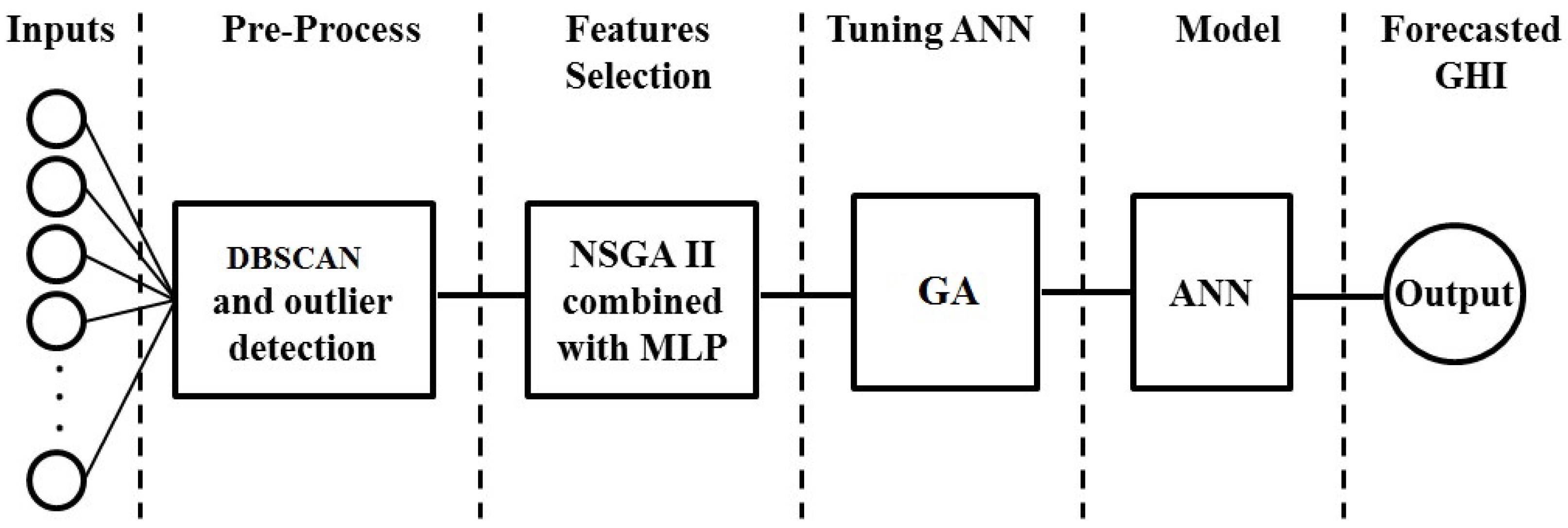
None of the articles mentioned above present a robust method for tuning the ANN and selecting the input parameters. Despite utilizing different machine learning algorithms in previous studies, there is no clear strategy for developing an algorithm which does not need an operator in all steps of the process. The aim of the present study was to develop an algorithm that takes the raw data and generates the results. While in previous studies, different hidden layer sizes, transfer functions, and numerous combinations of input parameters must be tested, in current research the whole process is automatic and has no need of human interference. This research used an MLP as the main algorithm and the parameters to be used as the inputs of the MLP were selected by the non-dominant sorted genetic algorithm II (NSGA II). Meanwhile, the MLP was tuned by a genetic algorithm (GA).
The rest of the paper is organized as follows: Section 2 describes the methodology, including the location from which data were collected and a brief explanation of the whole process. Section 3 describes the employed machine learning algorithms. The results are presented and discussed in Section 4. Finally, Section 5 summarizes the conclusions of the present study.

2. Methodology

2.1. Case Study

In this research, hourly meteorological raw data from 19 November 2010 to 18 November 2014 provided by the National Renewable Energies Laboratory (NREL) [11] for Elizabeth City (36°17′44″ N, 76°13′30″ W), North Carolina, USA, were used. A GHI map of the United States is given in Figure 1.
Measured hourly meteorological parameters include average roof temperature (ART), average roof wind chill temperature (ARWCT), average roof dew point temperature (ARDPT), average roof relative humidity (ARRH), average average wind speed (AAWS), average peak wind speed (APWS), average station pressure (ASP), average zenith angel (AZA), average azimuth angel (AAA), average airmass (AA), ACR data logger temperature (ACRT) and global horizontal irradiance (GHI). More information about the measuring instrument and station is given in [13]. Nine different delays of the GHI were defined as the probable inputs, and a new data table was created using parameters mentioned earlier and the defined delays of the GHI. Since the biggest defined delay was the measured value of 2 years ago, the target of the forecasting was GHI between 19 November 2012 and 18 November 2014. A figure of the measured values of the GHI from 19 November 2010 to 18 November 2014 was generated and is shown in Figure 2.

2.2. Proposed Algorithm

An MLPNN was utilized in order to obtain the forecasting results. The whole process is a hybrid algorithm which consists of density-based spatial clustering of applications with noise (DBSCAN) for removing noise and NSGA II for selecting the input parameters. Tuning of the MLPNN was conducted by GA. In both NSGA II and GA, the cost function is a multi-layer perceptron. The delays of the GHI for obtaining the future values follow Equation (1):
x ( k + h ) = f [ x ( k ) , x ( k 1 ) , x ( k 2 ) , , x ( k n ) ] ,
where k is the kth measured value and h is the forecasting horizon for the previous values of the x by function f, and n represents the maximum number of delays. The steps of the process for generating the forecasted value for the desired forecasting horizon are demonstrated in Figure 3 and described in Section 3 and Section 4.

3. Data Pre-Processing

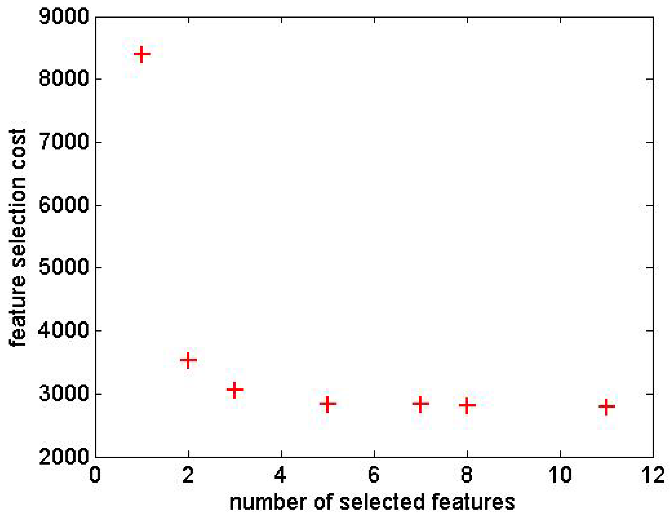
Collected raw data must be pre-processed and prepared to be used as the input of the MLPNN. The first step is anomaly detection. Some of the raw data might be of no use due to extraordinary climate changes or failure of the measuring equipment, and these data need to be eliminated. The employed anomaly detection technique for this study was DBSCAN. Following the detection and elimination of the anomalies (outliers), feature selection is considered to be the next step. Having used all the measured parameters as the inputs of the network, one may still not be successful in terms of accurate forecasting, and some of the parameters might not be useful. Furthermore, in the presence of computational restrictions, the suitable parameters must be selected to guarantee the accuracy of the forecasting. Therefore, the nature of the problem is a multi-objective optimization in which the primary objectives are higher accuracy and fewer input parameters. To help resolve this issue, one approach is the use of meta-heuristic algorithms such as particle swarm optimization (PSO), genetic algorithm (GA), ant colony optimization (ACO), etc. For each number of the parameters, the aforementioned algorithms randomly select the parameters by associating 0 or 1 to each one of them, then the process is repeated to the point of a stopping criterion. Another faster and more accurate approach is the use of multi-objective optimization algorithms. Considering that we are facing a multiple-criteria decision making problem, this study employed an NSGA II algorithm, which is recognized as one of the most widespread multi-objective optimization algorithms.

3.1. DBSCAN

Clustering is the practice of classifying similar objects together based on their similarities. The similarity might be limited to distance. Lloyd’s algorithm, mostly known as k-means, is a good example of this approach, where k is the number of clusters. Lloyd’s algorithm assumes that the best clusters are found by minimizing intra-cluster variance and maximizing the inter-cluster variance [14]. However, using distance-based algorithms does not necessarily guarantee the success of the clustering, particularly for high-dimensional data, where density-based clustering methods lead to better results. DBSCAN was introduced by Ester et al. [15], and is one the most effective density-based clustering algorithms. It is able to discover any number of clusters with different sizes and arbitrary shapes. DBSCAN assigns the points to the same cluster if they are density-reachable from one another. This algorithm has three inputs: set of points, neighborhood value (N), and minimum number of points in neighborhood (density).
DBSCAN starts by labeling the points as core, border, or noise points. The point with minimum points in its neighborhood is called a core point. The non-core point with at least one core point in its neighborhood is a border point, and all other points are noise points (outliers) and lie alone in low-density regions. The next step is assigning core and border points to clusters until all points are assigned to a cluster. It is important to note that DBSCAN is sensitive to neighborhood parameters. Choosing a small neighborhood value results in many points labeled as noise, and choosing a high value merges the dense clusters. Examples for core, border, and noise points are shown in Figure 4.
In the present research, the codes of the DBSCAN were developed in Matlab so as to detect and remove the data with noise from the data set. A previous study for anomaly detection based on DBSCAN can be found in [16], and more details and codes of the algorithm are given in [15].

3.2. NSGA II

The NSGA II algorithm was introduced by Deb et al. in 2002 [17] as an improved version of the NSGA [18]. It was utilized to solve various multi-objective optimization problems, including input selection [19]. NSGA II is a population-based algorithm and initializes with a random population. Then, population is sorted based on the value of the cost function in non-dominant order in each front, where individuals in the first front ( F 1 ) are non-dominant by other individuals, and the second front ( F 2 ) contains dominated individuals in the population in each iteration.
The GA operators of selection, crossover, and mutation are the next steps of the algorithm. The selection is a binary tournament selection, and is based on the crowding distance and cost value. Higher crowding distance demonstrates higher population diversity. Offspring is created by crossover and mutation operators, and the best N individuals of the offspring population are selected and sorted in non-dominant order. NSGA II depends on parameters like population size, number of iterations, crossover probability, and mutation probability. Some indications to set these parameters are given in [20].
The algorithm for the non-dominated sort is given in Algorithm 1, where p, P, and Q are the individuals, parent vector, and the offspring vector, respectively. S p contains the individuals dominated by p, n p is the number of individuals that dominate p, and i is the number of the ith front.
The procedure for calculating the crowding distance is shown in Algorithm 2. As seen in Algorithm 2, the boundaries have infinite distance and m is the number of the mth objective function of the ith individual in I. The selection is based on the calculated crowding distance, and after applying crossover and mutation operators, the final step is recombination and selection. To ensure the elitism, the next generation is the combination of the best individuals from the parent vector and offspring vector. The process subsequently repeats to generate the individuals of the next generations, and stops when the stopping criteria is satisfied.
Algorithm 1 Non-dominated sort
  • for each ρ ϵ P do
  •      S ρ = ϕ
  •      n ρ = 0
  •     for each q ϵ P do
  •         if ρ < q then
  •             S p = S p { q }
  •         else(q < ρ )
  •             n p = n p + 1
  •         end if
  •         if n ρ = 0 then
  •             ρ r a n k = 1
  •             F 1 = F 1 { ρ }
  •         end if
  •     end for
  • end for
  • i = 1
  • while F 1 ϕ do
  •     Q = ϕ
  •     for each ρ ϵ F i do
  •         for each q ϵ S ρ do
  •             n q = n q 1
  •            if n q = 0 then
  •                 q r a n k = i+1
  •                Q = Q ϵ { q }
  •            end if
  •         end for
  •     end for
  •     i = i + 1
  •      F i = Q
  • end while
Algorithm 2 Crowding distance
H
  • l = I
  • for each i, set I [ i ] d i s t a n c e = 0 do
  •     for each objective m do
  •         I = Sort { I , m }
  •          I [ 1 ] d i s t a n c e = I [ l ] d i s t a n c e =
  •         for i = 2 to (l-1) do
  •             I [ i ] d i s t a n c e = I [ i ] d i s t a n c e + ( I [ i + 1 ] . m I [ i 1 ] . m ) / ( f m m a x f m m i n )
  •         end for
  •     end for
  • end for

4. MLPNN

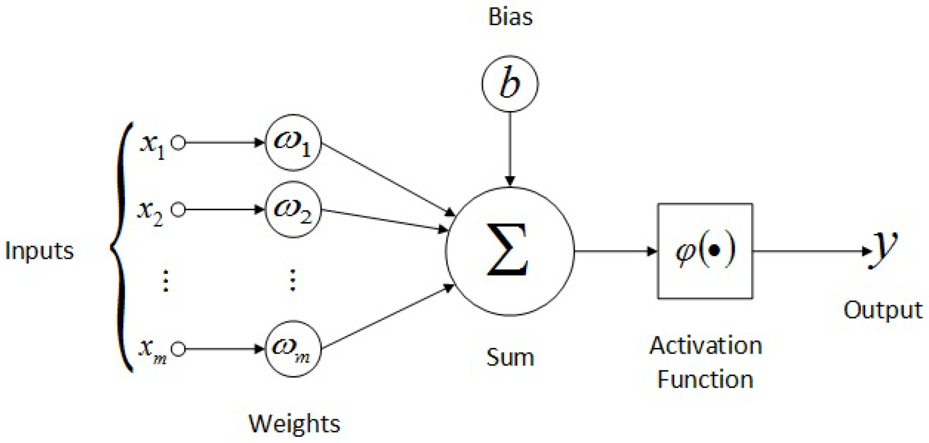
As mentioned above, this work employed multi-layer perceptron neural network (MLPNN) to forecast the GHI. An MLP consists of an input layer, at least one hidden layer, and an output layer. Each layer contains processing units (neurons) that perform operations on their input data and send it to the following layers. The number of neurons in input layer is equal to the number of the input variables. In this work, the output layer has one neuron because of the only one desired output (i.e., forecasted GHI). The major challenge lies in choosing the proper number of the neurons in the hidden layer. Furthermore, it must be considered that each input is first multiplied by the corresponding weight parameter and the resulting product is added to a bias to produce a weighted sum [21]. The resulted weighted sum of each neuron passes through a neuron activation function (i.e., transfer function) to produce the final output of the neuron. The most common activation functions are provided in Table 1, and the structure of an artificial neuron is shown in Figure 5.
The process of the adaptation of the weights is known as the training stage. There are several training algorithms, each applied to different neural network models, and the main difference among them is how the weights are adjusted. The present study utilized supervised learning with the back-propagation training algorithm, which iteratively reduces the difference between the obtained and desired output using a minimum error as reference. In this method, the weights are adjusted between the layers by means of the back-propagation of the error found in each iteration.
The tuning discussed in this work, which is realized by the GA and PSO algorithm, consists of choosing the proper hidden layer size and the proper activation function.

4.1. PSO

PSO was developed by James Kennedy and Russell Eberhart in 1995 [22] and was inspired by the flocking and schooling patterns of birds. It is recognized as a powerful population-based algorithm for optimization. The algorithm is initialized by random particles, and the initial population creates the swarm as presented in Equation (2):
X = x 1 , x 2 , , x N .
Unlike algorithms such as GA, PSO does not use selection, and all particles can share information about the search space. Each particle moves in an D-dimensional space and contains a position and a velocity. The position of each particle is described in Equation (3):
x i = [ x i 1 x i 2 x i 3 x i D ] .
Velocity controls the exploration, and cannot exceed the maximum allowed speed ( v m a x ( j ) ). Maximum velocity controls the exploration. Low values result in local exploration, whereas higher values of the maximum velocity cause global exploration. Velocity is adjusted using Equation (4):
v i j = v i j ( t + 1 ) , if v i j ( t + 1 ) < v m a x ( j ) , v m a x ( j ) otherwise .
Equations (5) and (6) are used to determine the minimum and maximum velocity to the solution:
v m a x , j = δ ( x m a x , j x m i n , j ) ,
v m i n , j = δ ( x m i n , j x m a x , j ) .
x m a x , j and x m i n , j are the minimum and maximum positions of the particle in the jth dimension, and δ is a constant between 0 and 1.
The particles keep a record of the position of its best performance. Meanwhile, the best value obtained by all particles is stored as the global best. All particles can share information about the search space, and each particle calculates its velocity based on its best performance and the global best. By using this velocity, the particles update their position at each iteration, which is calculated by Equation (7):
V i ( t + 1 ) = w × V i t + c 1 ( p i x i t ) R 1 + c 2 ( g x i t ) R 2 ,
where w is the inertial weight, p 1 is the personal best, and g is the global best. t and t + 1 indicate two successive iterations of the algorithm, and v i is the vector of velocity components of the ith particle. c 1 and c 2 are constant values. Some approaches to set w, c 1 , and c 2 are discussed in [23].
The trajectory of particles towards the optimal solution is defined as Equation (8):
x i ( t + 1 ) = x i ( t ) + v i ( t + 1 ) .

4.2. GA

GA is a meta-heuristic algorithm inspired by evolution of chromosomes and natural selection. It was introduced by John Holland in 1960 [24], and has been found to demonstrate good performance in solving non-linear optimization problems. GA is originally a binary coded algorithm, and it can be used for solving continuous space problems by applying some modifications to its operators [25]. The GA used in this research is a continuous GA. It starts with an initial population, and after assigning a fitness value for each chromosome, new chromosomes (offspring) are created from the previous chromosomes (parents), which have better fitness values. Selection of the parents can be done by many techniques, such as roulette-wheel selection, tournament selection, and elitist selection. In the next step, genetic operations of mutation and crossover are applied to the selected chromosomes to generate the offspring. Crossover is the process of dividing two randomly selected chromosomes with the best fitness value and exchanging them to produce new offspring. Various crossover approaches for continuous GA are given in [26,
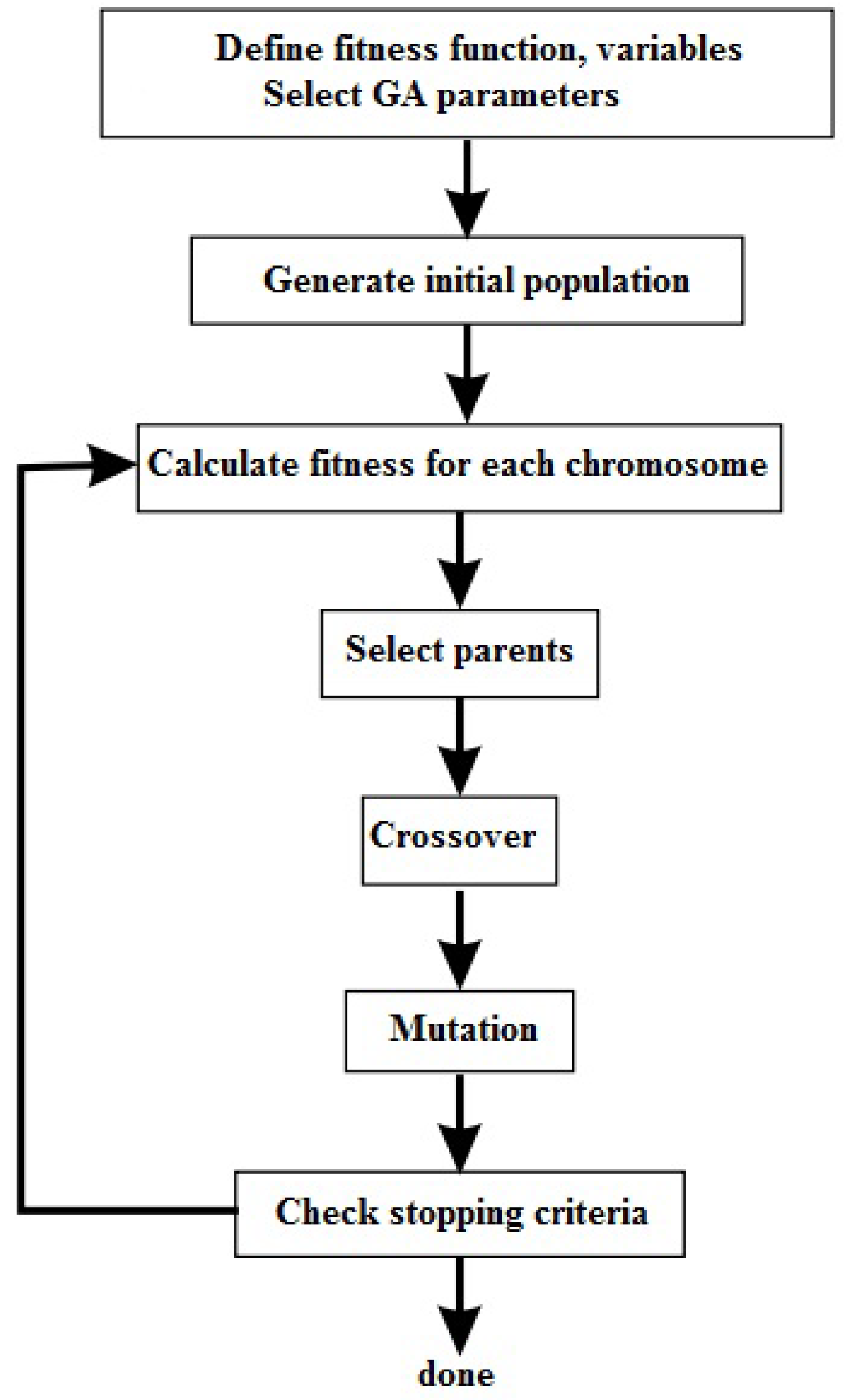
27]. Mutation is randomly changing a part of a selected chromosome based on the defined mutation rate, which causes a random change in exploring the solution space. Without mutation, GA converges rapidly and this causes a tendency to converge to a local optimum.
Finally, the generated new population (chromosomes) passes through evaluation and calculation of the fitness value. These steps repeat in each iteration until a termination criterion is satisfied. A flowchart of the continuous GA is shown in Figure 6.

5. Results and Discussion

5.1. Outlier Detection

The measured data for each variable were checked to detect the noise (outliers) using the DBSCAN algorithm. Once the outliers were detected, they were subsequently removed from the dataset. Since the noise has a negative effect on forecasting accuracy, this process is of vital importance so as to detect and remove the noise in order to obtain more precise forecasting results. Forecasting performance before and after noise reduction is presented in Table 2. It must be noted that the reported values in Table 2 and all other tables related to the results are for the test data set. In addition, before tuning the network, the number of neurons in the hidden layer and transfer functions were set to 20 and hyperbolic tangent sigmoid, respectively.

5.2. Feature Selection

All measured meteorological data together with defined previous values of the GHI were fed to the NSGA II algorithm as the inputs. The cost function of the algorithm is an ANN and the fitness of the algorithm is the combination of the mean squared error (MSE) of the testing and training data sets of the ANN. Five different fitnesses (cost function) with different weights for testing and training data sets were tested. Furthermore, to avoid the effect of the probable unsuccessful runs, an upper bound was defined for the MSE values of the cost function. RMSE, normalized RMSE (nRMSE), and R related to each test in presented in Table 3. The reported results were related to the solution with the best RMSE in each case, and in order to gain robust results, the fitness was set to be the mean of five runs. Maximum number of iterations, population size, crossover probability, and mutation probability were set to 50, 50, 0.7, and 0.4, respectively. As can be seen, the cost function with relative weight of the 0.5 for the test data set and 0.5 for the train data set was found to generate better results.
The Pareto front of the NSGA II related to the chosen cost function is shown in Figure 7. As discussed in Section 3, despite algorithms like PSO, GA, ACO, etc. that generate only one solution, all seven members of the Pareto front of the NSGA II were the solutions of the problem.
To select the proper solution to work, the computational power, cost, and desired quality of the forecasting must be taken into account. If forecasting accuracy is of top priority, the solution with better nRMSE and nMAE must be employed. Otherwise, other generated solutions might be considered. Selected inputs related to the generated solutions are presented in Table 4.
As seen in Table 4, the first previous value of the GHI (GHI-1) was selected in all solutions, and it demonstrates the importance of this variable in the forecasting process. Table 5 demonstrates the forecasting results for each member of the Pareto front (solution) generated by NSGA II.

5.3. MLPNN Tuning

The algorithm used in this paper is a continuous GA, which was designed to solve continuous space problems. Therefore, some adaptations were necessary to employ this algorithm for tuning purposes. The algorithm is supposed to choose the size of the hidden layer (an upper bound of 20 was defined for the current work) as well as two transfer functions for the network. As observed, the current problem is not of continuous type, so in order to tackle this, numbers 1 to 20 were associated with hidden layer size and numbers 1 to 3 were associated with the purelin (linear), logsig (logistic sigmoid), and tansig (hyperbolic tangent sigmoid) transfer functions, respectively. The individuals generated by GA and the positions of the particles of the PSO algorithm in each iteration were rounded, and the product which was a number between 1 and 20 for the hidden layer size was used to determine the number of neurons, and numbers between 1 and 3 for determining the transfer functions. The fitness of each iteration was calculated by an MLPNN. As in feature selection, fitness was set to be the mean of five runs and an upper bound of MSE was defined to reduce the effect of the unsuccessful runs in the results. We utilized the ability of GA to generate solutions and the ability of the PSO algorithm to explore the solution space. GA was found to have a better performance in comparison with PSO. The values for the parameters of the PSO and GA are given in Table 6.
The variation of the fitness in each iteration of GA and PSO is shown in Figure 8.
The network tuning results obtained by GA and PSO algorithms are presented in Table 7.

5.4. Forecasting Results

As the final steps, the tuned MLPNN was fed by selected features. The final results for each network tuned by GA and PSO algorithms are given in Table 8. As seen in table, proper tuning of the MLPNN resulted in a reduction of error in terms of all indicators of the RMSE, nRMSE, MAE, nMAE, and R. In all steps of using the MLPNN, 70% of the data were used for training and 30% of the data were used as validation and testing data.
The outputs of GA–MLPNN and PSO–MLPNN for a study region of 24 h is shown in Figure 9. The same study regions of the 4 days and 1 week are presented in Figure 10 and Figure 11, respectively, and as can be seen, outputs of the both networks were very close to the measured values of the GHI. However, the neural network tuned by GA demonstrated better results.

6. Conclusions

Switching to renewable energy is unavoidable due to various problems caused by generating energy with fossil fuels and nuclear power plants. Among renewable sources, solar energy makes it possible to generate energy with different methods. PV solar energy is one of the methods which is currently of great importance due to its clean and environmentally friendly characteristics as well as decreasing PV cell prices. However, there is still much ongoing research aiming to overcome the challenges caused by PV systems. The current study is dedicated to developing a methodology to make the forecasting of the GHI more reliable. By using the developed methodology, there is no need to adapt new data sets to the currently existing algorithms or to tune the neural network by a trial and error approach. Since the the developed methodology employs an input selection algorithm, it generates results with any given data set containing different variables. Once the inputs are selected and the neural network is trained and tuned, the algorithm is ready to use without any computational complexities.
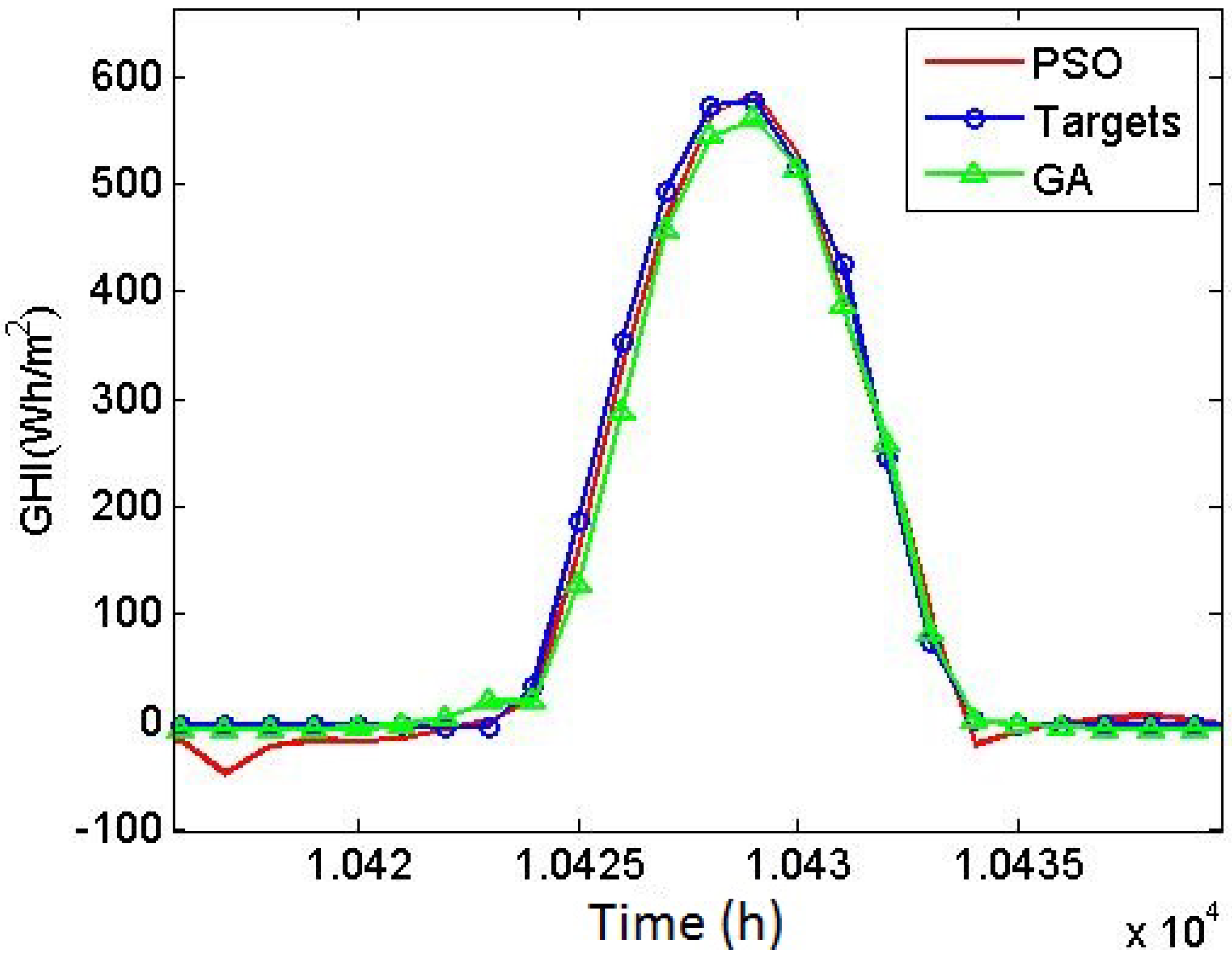
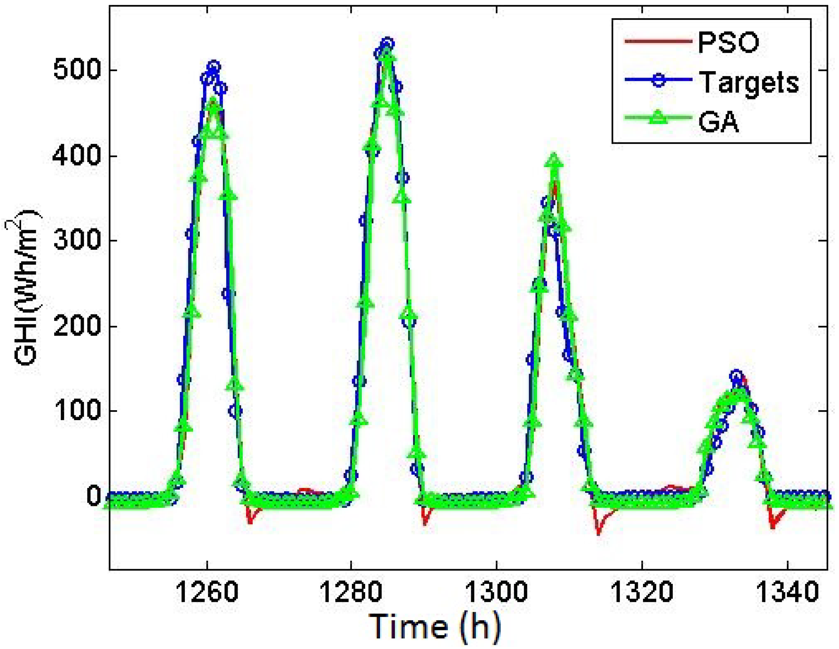
In this paper, a combination of different machine learning techniques were used to forecast the GHI. Anomalies were detected and removed by DBSCAN, and features were selected by NSGA II. A multi-layer perceptron neural network was employed to forecast the hourly GHI, and the tuning of the network was realized by GA, which demonstrated good performance in generating solutions in the explored solution space. This study proves the better performance of the GA over PSO algorithm in terms of the tuning of neural networks.
The uniqueness of this approach lies in employing NSGA II for selecting the inputs of the MLPNN and adapting GA for tuning of the neural network. In previous studies that employed artificial neural networks, there are no specific approaches for addressing these issues.
The validity of the developed model was tested using the data set for Elizabeth City, North Carolina, USA, and the error rates constantly reduced in each stage of applying the methodology. Using this specific data set, the study achieved an nRMSE value of 0.0458, an nMAE value of 0.0238, and a correlation coefficient of 0.9884.

Author Contributions

A.J. was responsible for developing the methodology, analyzing data, and generating results. R.M. and N.d.S. edited and re-wrote the manuscript drafts and participated in generating results. A.C.d.C.L. supervised the research, corrected, and approved the submitted manuscript.

Funding

This research has been funded by the Coordination for the Improvement of Higher Education Personnel (CAPES).

Conflicts of Interest

The authors declare no conflict of interest.

Abbreviations

ACOAnt Colony Optimization
ANFISAdaptive Neuro-Fuzzy Inference System
ANNArtificial Neural Network
DBSCANDensity-Based Spatial Clustering for Applications with Noise
DNIDirect Normal Irradiance
GAGenetic Algorithm
GHIGlobal Horizontal Irradiance
MAEMean Absolute Error
MBEMean Bias Error
MLPNNMulti-Layer Perceptron Neural Network
MSEMean Squared Error
NSGA IINon-Dominated Sorting Genetic Algorithm II
PSOParticle Swarm Optimization
PVPhotovoltaic
RCorrelation Coefficient
RBFRadial Basis Function
RMSERoot Mean Square Error
SVRSupport Vector Regression

Appendix A

The indicators of root mean squared error (RMSE), normalized root mean squared error (nRMSE), mean absolute error (MAE), normalized mean absolute error (nRMSE) and correlation coefficient (R) were used for evaluations of the model. The following equations describe these indicators:
R M S E = 1 n i = 1 n ( x i y i ) 2
n R M S E = R M S E x m a x x m i n
M A E = 1 n i = 1 n x i y i
n M A E = M A E x m a x x m i n
R = i = 1 n ( x i x ¯ ) ( y i y ¯ ) i = 1 n ( x i x ¯ ) 2 i = 1 n ( y i y ¯ ) 2
where, x i and x i ¯ are the measured value and mean of the measured value for the GHI and y i and y i ¯ are the forecasted value and mean of the forecasted value for the GHI respectively.

References

  1. Rajgor, G. Greater acceleration of renewables required to meet COP21 goal. Renew. Energy Focus 2016, 17, 175–177. [Google Scholar] [CrossRef]
  2. Qazi, A.; Fayaz, H.; Wadi, A.; Raj, R.G.; Rahim, N.; Khan, W.A. The artificial neural network for solar radiation prediction and designing solar systems: A systematic literature review. J. Clean. Prod. 2015, 104, 1–12. [Google Scholar] [CrossRef]
  3. Wang, Z.; Wang, F.; Su, S. Solar Irradiance Short-Term Prediction Model Based on BP Neural Network. Energy Procedia 2011, 12, 488–494. [Google Scholar] [CrossRef]
  4. Chiteka, K.; Enweremadu, C. Prediction of global horizontal solar irradiance in Zimbabwe using artificial neural networks. J. Clean. Prod. 2016, 135, 701–711. [Google Scholar] [CrossRef]
  5. Khosravi, A.; Koury, R.; Machado, L.; Pabon, J. Prediction of hourly solar radiation in Abu Musa Island using machine learning algorithms. J. Clean. Prod. 2018, 176, 63–75. [Google Scholar] [CrossRef]
  6. Hejase, H.A.; Al-Shamisi, M.H.; Assi, A.H. Modeling of global horizontal irradiance in the United Arab Emirates with artificial neural networks. Energy 2014, 77, 542–552. [Google Scholar] [CrossRef]
  7. Renno, C.; Petito, F.; Gatto, A. {ANN} model for predicting the direct normal irradiance and the global radiation for a solar application to a residential building. J. Clean. Prod. 2016, 135, 1298–1316. [Google Scholar] [CrossRef]
  8. Gutierrez-Corea, F.V.; Manso-Callejo, M.A.; Moreno-Regidor, M.P.; Manrique-Sancho, M.T. Forecasting short-term solar irradiance based on artificial neural networks and data from neighboring meteorological stations. Sol. Energy 2016, 134, 119–131. [Google Scholar] [CrossRef]
  9. Mellit, A.; Pavan, A.M. A 24-h forecast of solar irradiance using artificial neural network: Application for performance prediction of a grid-connected {PV} plant at Trieste, Italy. Sol. Energy 2010, 84, 807–821. [Google Scholar] [CrossRef]
  10. Amrouche, B.; Pivert, X.L. Artificial neural network based daily local forecasting for global solar radiation. Appl. Energy 2014, 130, 333–341. [Google Scholar] [CrossRef]
  11. National Renewable Energy Laboratory (NREL) Home Page. Available online: http://www.nrel.gov/ (accessed on 4 April 2017).
  12. Solar Resource Map © 2018 Solargis. (1200×872). Under License (CC BY SA 4.0) http://creativecommons.org/licenses/by-sa/4.0/ Available online: https://solargis.com/maps-and-gis-data/download/usa (accessed on 4 July 2018).
  13. Elizabeth City State University. Available online: https://midcdmz.nrel.gov/apps/go2url.pl?site=EC (accessed on 4 April 2017).
  14. Arbelaitz, O.; Gurrutxaga, I.; Muguerza, J.; Pérez, J.M.; Perona, I. An extensive comparative study of cluster validity indices. Pattern Recognit. 2013, 46, 243–256. [Google Scholar] [CrossRef]
  15. Ester, M.; Kriegel, H.P.; Sander, J.; Xu, X. A Density-Based Algorithm for Discovering Clusters in Large Spatial Databases with Noise. In Proceedings of the Second International Conference on Knowledge Discovery and Data Mining (KDD-96), Portland, OR, USA, 2–4 August 1996. [Google Scholar]
  16. Celik, M.; Dadaşer-Celik, F.; Dokuz, A.S. Anomaly detection in temperature data using DBSCAN algorithm. In Proceedings of the 2011 International Symposium on Innovations in Intelligent Systems and Applications, Istanbul, Turkey, 15–18 June 2011; pp. 91–95. [Google Scholar] [CrossRef]
  17. Deb, K.; Pratap, A.; Agarwal, S.; Meyarivan, T. A fast and elitist multiobjective genetic algorithm: NSGA-II. IEEE Trans. Evolut. Comput. 2002, 6, 182–197. [Google Scholar] [CrossRef] [Green Version]
  18. Srinivas, N.; Deb, K. Muiltiobjective Optimization Using Nondominated Sorting in Genetic Algorithms. Evolut. Comput. 1994, 2, 221–248. [Google Scholar] [CrossRef] [Green Version]
  19. Anemangely, M.; Ramezanzadeh, A.; Tokhmechi, B. Shear wave travel time estimation from petrophysical logs using ANFIS-PSO algorithm: A case study from Ab-Teymour Oilfield. J. Nat. Gas Sci. Eng. 2017, 38, 373–387. [Google Scholar] [CrossRef]
  20. Li, H.; Zhang, Q. Multiobjective Optimization Problems With Complicated Pareto Sets, MOEA/D and NSGA-II. IEEE Trans. Evolut. Comput. 2009, 13, 284–302. [Google Scholar] [CrossRef]
  21. Farajzadeh, J.; Fard, A.F.; Lotfi, S. Modeling of monthly rainfall and runoff of Urmia lake basin using “feed-forward neural network” and “time series analysis” model. Water Res. Ind. 2014, 7–8, 38–48. [Google Scholar] [CrossRef]
  22. Kennedy, J.; Eberhart, R.C. Particle swarm optimization. In Proceedings of the 1995 IEEE International Conference on Neural Networks, Perth, WA, Australia, 27 November–1 December 1995; pp. 1942–1948. [Google Scholar]
  23. Rini, D.P.; Shamsuddin, S.M.; Yuhaniz, S.S. Particle Swarm Optimization: Technique, System and Challenges. Int. J. Comput. Appl. 2011, 14, 19–27. [Google Scholar] [CrossRef]
  24. Holland, J.H. Adaptation in Natural and Artificial Systems; University of Michigan Press: Ann Arbor, MI, USA, 1975. [Google Scholar]
  25. Chelouah, R.; Siarry, P. A Continuous Genetic Algorithm Designed for the Global Optimization of Multimodal Functions. J. Heuristics 2000, 6, 191–213. [Google Scholar] [CrossRef]
  26. Adewuya, A.A. New Methods in Genetic Search with Real-Valued Chromosomes. Master’s Thesis, Department of Mechanical Engineering, Massachusetts Institute of Technology, Cambridge, MA, USA, 1996. [Google Scholar]
  27. Michalewicz, Z. Genetic Algorithms + Data Structures = Evolution Programs; Springer: Berlin/Heidelberg, Germany, 1994. [Google Scholar]
Figure 1. GHI map of the United States [12].
Energies 11 02641 g001
Figure 2. Measured values of global horizontal irradiance (GHI) in Elizabeth City, North Carolina, USA from 19 November 2010 to 18 November 2014.
Energies 11 02641 g002
Figure 3. Description of the proposed algorithm. ANN: artificial neural network; DBSCAN: density-based spatial clustering of applications with noise; GA: genetic algorithm; NSGA II: non-dominant sorted genetic algorithm II.
Energies 11 02641 g003
Figure 4. Example for core, border, and noise points (MinPts = 4).
Energies 11 02641 g004
Figure 5. Structure of an artificial neuron.
Energies 11 02641 g005
Figure 6. Flowchart of the continuous GA.
Energies 11 02641 g006
Figure 7. Pareto front of NSGA II.
Energies 11 02641 g007
Figure 8. Fitness in each iteration of GA and PSO.
Energies 11 02641 g008
Figure 9. Forecasting results for the region of 24 h.
Energies 11 02641 g009
Figure 10. Forecasting results for a 4-day period.
Energies 11 02641 g010
Figure 11. Forecasting results for a 1-week period.
Energies 11 02641 g011
Table 1. The most common activation functions.
DescriptionEquation
Linear ϕ ( z ) = z
Logistic sigmoid ϕ ( z ) = 1 1 + e z
Hyperbolic tangent sigmoid ϕ ( z ) = e z + e z e z + e z
Table 2. Results with raw data and data after outlier detection.
Dataset RMSE Ts ( Wh / m 2 ) nRMSE Ts MAE Ts ( Wh / m 2 ) nMAE Ts R Ts
Raw data59.06970.056832.53030.03130.9741
Data without noise55.00390.052927.74680.02670.9765
Table 3. RMSE, nRMSE, and R related to the tested cost functions.
Cost Function RMSE Ts ( Wh / m 2 ) nRMSE Ts R Ts
0.2( MSE Tr ) + 0.8( MSE Ts )54.82960.05270.9775
0.4( MSE Tr ) + 0.6( MSE Ts )52.68340.05060.9782
0.5( MSE Tr ) + 0.5( MSE Ts )50.38650.04840.9807
0.6( MSE Tr ) + 0.4( MSE Ts )53.29560.05120.9782
0.8( MSE Tr ) + 0.2( MSE Ts )54.52590.05240.9779
Table 4. Selected inputs related to the solutions generated by NSGA II.
SolutionSelected Inputs
11 Features(GHI-1), (GHI-3), ARWCT, ARDPT, ARRH, AAWS, APWS, AZA, AAA, AA, ACRT
8 Features(GHI-1), ARWCT, ARRH, APWS, AZA, AAA, AA, ACRT
7 Features(GHI-1), ARWCT, ARRH, APWS, AZA, AAA, ACRT
5 Features(GHI-1), ARRH, AZA, AAA, ACRT
3 Features(GHI-1), AZA, AAA
2 Features(GHI-1), AAA
1 Feature(GHI-1)
Table 5. Forecasting error for the each member of the Pareto front generated by NSGA II.
Dataset RMSE Ts ( Wh / m 2 ) nRMSE Ts MAE Ts ( Wh / m 2 ) nMAE Ts R Ts
11 Features50.38650.048425.61410.02460.9807
8 Features51.35360.049425.41140.02440.977
7 Features51.36940.049427.57490.02650.9769
5 Features54.56320.052526.96510.02590.9735
3 Features55.46230.053326.29730.02530.9735
2 Features56.2770.054129.28820.02810.972
1 Feature94.73650.091157.50430.05530.9215
Table 6. Values for the parameters of particle swarm optimization (PSO) and GA.
PSO ParametersGA Parameters
C1 = 1.4962pCrossover = 0.7
C2 = 1.4962pMutation= 0.2
w = 0.7298nMutation = 10
MaxIt = 50MaxIt = 50
nPop = 50nPop = 50
Table 7. Network tuning results obtained by GA and PSO algorithms.
Tuning AlgorithmHidden Layer SizeTransfer Function 1Transfer Function 2
PSO12tansigpurelin
GA15tansigtansig
Table 8. Results after tuning the ANN.
Dataset RMSE Ts ( Wh / m 2 ) nRMSE Ts MAE Ts ( Wh / m 2 ) nMAE Ts R Ts
Tuned by PSO47.94140.0461326.2890.02520.9786
Tuned by GA47.69550.045824.77720.02380.9884

