Formulation of the Phasors of Apparent Harmonic Power: Application to Non-Sinusoidal Three-Phase Power Systems
by
 , ,
, ,
Pedro A. Blasco
1 ,
,
Rafael Montoya-Mira
1,
José M. Diez
1,*,
Rafael Montoya
1 and
Miguel J. Reig
2 1
Departamento de Ingeniería Eléctrica, Universitat Politècnica de València, Plaza Ferrandiz y Carbonell s/n, 03801 Alcoy, Spain
2
Departamento de Ingeniería Mecánica y Materiales, Universitat Politècnica de València, Plaza Ferrandiz y Carbonell s/n, 03801 Alcoy, Spain
*
Author to whom correspondence should be addressed.
Energies 2018, 11(7), 1888; https://doi.org/10.3390/en11071888
Submission received: 27 June 2018
/
Revised: 12 July 2018
/
Accepted: 16 July 2018
/
Published: 19 July 2018
(This article belongs to the Section F: Electrical Engineering)
Abstract
:In this work, the expression of the phasor of apparent power of harmonic distortion is formulated in the time domain. Applying this phasor along with the phasor of apparent unbalance power allows us to obtain a new set of phasors that include all of the inefficient power components appearing in the transfer of energy in non-linear and unbalanced systems. In this manner, a new model of inefficient power in electrical systems is developed. For each voltage harmonic of order ‘m’ and current harmonic of order ‘n’, a phasor of harmonic apparent power is obtained. Accuracy in the determination of the total apparent power of a system depends on the number of harmonics considered. Each phasor of apparent harmonic power is formed from six mutually orthogonal parameters or components that are calculated from the harmonic voltages at the nodes of the network and the circulating harmonic currents. To demonstrate the validity of the proposed formulation, a four-wire non-linear system formed by two nodes is assessed.
1. Introduction
In addition to useful power for the transfer of energy (or active power), the power generated by a three-phase electrical system includes non-useful components that must be taken into account in the analysis of energy transfer [1]. Phase differences between voltage and current result in reactive power [2], and an unbalanced three-phase electrical system produces a so-called power of unbalance [3]. In addition, such electrical systems are designed to work with voltages and sinusoidal currents, and the use of non-linear loads and/or variants over time distorts the voltage and current waveforms, resulting in the creation of harmonic components. The analysis of the generation and propagation of harmonic components through an electrical system is called harmonic power flow analysis [4].
These types of non-useful power can be critically detrimental to an electrical system through their effects on the operation of protection and measuring equipment, which can result in unexpected opening and erroneous measurement [5,6]. In addition, increased currents can enhance power losses in transmission lines [7] and in motors can cause winding overheating; loss of thermal insulation, copper and iron; reduction in the motor torque; decrease in performance, etc. [8]. In generators, non-useful components can hinder automatic synchronization with the network, and in neutral conductors they produce dangerous overheating because they add harmonic currents of the third-order (or integer multiples thereof). The physical significance of non-useful power components has been widely discussed in the scientific literature [9,10,11,12].
Non-linear loads are increasingly used in general applications, including switch mode power supplies, motors and variable speed drives, photocopiers, personal computers, laser printers, fax machines, battery chargers, etc. There is also currently a high amount of government support for the development of power generation using photovoltaic technology. Solar plants are considered to be an important source of harmonics as a result of the power electronics technology used in the electricity generation process [13,14,15]. The non-linear loads and solar energy sourcing has therefore increased the overall harmonic power present in electrical systems.
Harmonic power has also been widely discussed in the literature [16,17,18], with most recent studies focusing on the development of active filters to mitigate the effects of harmonic components [19,20,21,22,23,24]. Other research focuses on the development of techniques to assess and differentiate the harmonic contribution of customers and networks [25,26]. In these contributions, the harmonic power of the system is not evaluated phasorially. Currently, electrical power expressions developed in IEEE Std. 1459–2010 [10], obtained in the time domain, are accepted as valid, although approaches in the frequency domain are also possible [27]. Under the time-domain standard, harmonic current and voltage distortion rates (THDi and THDv, respectively) are established as proportions of the fundamental components and are expressed as percentages of the respective components.
In 2016, the authors of this paper defined the unbalance power phasor [28] and developed an equivalent circuit for the analysis of unbalance power in three-wire electrical systems [29]. The unbalance power and apparent power phasors of the positive sequence can be combined to produce the apparent power phasor of an unbalanced linear electrical system; this phasor has a modulus equivalent to that obtained by Buchholz [30] and IEEE Std. 1459–2010 [10].
This paper extends the method used in the formulation of the unbalance power phasor [28] to non-linear systems for calculating the harmonic distortion power. This application to non-linear power systems is not immediate. In this case, there are voltage and current harmonics of the same order, as well as of a different order. This gives rise to different harmonic powers, depending on the harmonic order of voltage and current that is considered. In this work, these powers are formulated phasorially.
The main advantage of the proposed method is that it allows analysis by phasor components. This allows us to obtain a new set of phasors that encompasses all balanced, unbalanced, sinusoidal or non-sinusoidal inefficient power components appearing in the transfer of energy in an electrical system in an approach that maintains all of the advantages of the phasor formulation.
The difference compared to the methods listed in the literature, mainly the IEEE Std. 1459–2010 [9], is that it only determines the harmonic powers in absolute values. This value matches with the module of the phasor proposed in this work. Moreover, another added advantage, presented by the phasor of apparent harmonic power, is that it allows us to know the contribution of each load to each of the mentioned harmonic powers at any point in the network.
The proposed procedure is not intended to replace the procedure established in IEEE Std. 1459-2010 but instead represents a new approach to understanding the inefficient power in an electrical system from a time-domain-based perspective.
The rest of this paper is organized as follows. In Section 2, the production of instantaneous power in non-linear systems is reviewed. In Section 3, the phasor of apparent harmonic power is formulated for a three-phase system with balanced voltages and non-linear loads. In Section 4, the apparent harmonic power phasor for a three-phase system with unbalanced voltages and non-linear loads is analyzed. In Section 5, the total apparent power of an electrical system and its modulus are analyzed. To aid in the understanding of the proposed calculation method and its application, Section 6 examines a case involving a system with unbalanced voltages and non-linear loads.
2. Review of Instantaneous Power in a Non-Sinusoidal System
The voltage and instantaneous current in a non-sinusoidal single-phase system are given by the following equations:
where
- m is the harmonic order of the voltage and n is the harmonic order of the current.
- and are, respectively, the voltage and current constant terms. In alternating-current power systems, these values are generally very small and, therefore, will not be considered further in this work.
- and are the root mean square (RMS) values for the harmonic voltage and harmonic current of orders m and n, respectively.
- and are the phase angle harmonic voltage and phase angle harmonic current of orders m and n, respectively.
The instantaneous power is given by the following equation:
where the first term, , is the instantaneous active power, which is decomposed into three instantaneous components:
Here, is the fundamental instantaneous active power, which is calculated as
This expression has two terms: the fundamental active power , and the oscillating component . The first term is equal to the average value of and determines the active power caused by the fundamental harmonics of voltage and current. The second term, which has an average value of zero, is always present when net energy is transferred to the load; however, it does not cause power loss in the conductors.
The second term in (4), , is the harmonic instantaneous active power of order h for h ≠ 1, and is calculated as
This term is caused by harmonic voltages of order h and harmonic currents of order h, that is, for harmonics of equal voltage and current, and has a value of zero for a linear electrical system.
The first term in (6) represents the sum of the harmonic active power components . The sum is equal to the average value of and the sum of and is the total active power of a non-sinusoidal electrical system. The second term of (6) represents the sum of oscillating harmonic components of amplitude and a frequency of 2h. The average value of the second term is zero, and the term does not correspond to power loss in the conductors.
The third term in (4), , is the harmonic instantaneous active power, which is caused by the harmonic voltage of order m and the harmonic current of order n, where m ≠ n. This term is calculated as
The average value of is zero.
The second term in (3), , is the instantaneous reactive power, which is also decomposed into three instantaneous components:
where
- is the fundamental instantaneous reactive power, which is calculated from (9).
- is harmonic instantaneous reactive power of order h ≠ 1, which is calculated from (10). This power component is caused by the harmonic voltage and harmonic current of orders h and h, respectively.
- is harmonic instantaneous reactive power, which is caused by the harmonic voltage of order m and the harmonic current of order n, where m ≠ n. This power is calculated from (11).
In a non-sinusoidal three-phase system, the instantaneous power and its components are expressed by the following equation:
For each of the phases (a, b and c), the instantaneous active power and the instantaneous reactive power are calculated from (4)–(7) and (8)–(11), respectively.
3. Harmonic Power in a Non-Linear Three-Phase Power System with Non-Sinusoidal Balanced Voltages
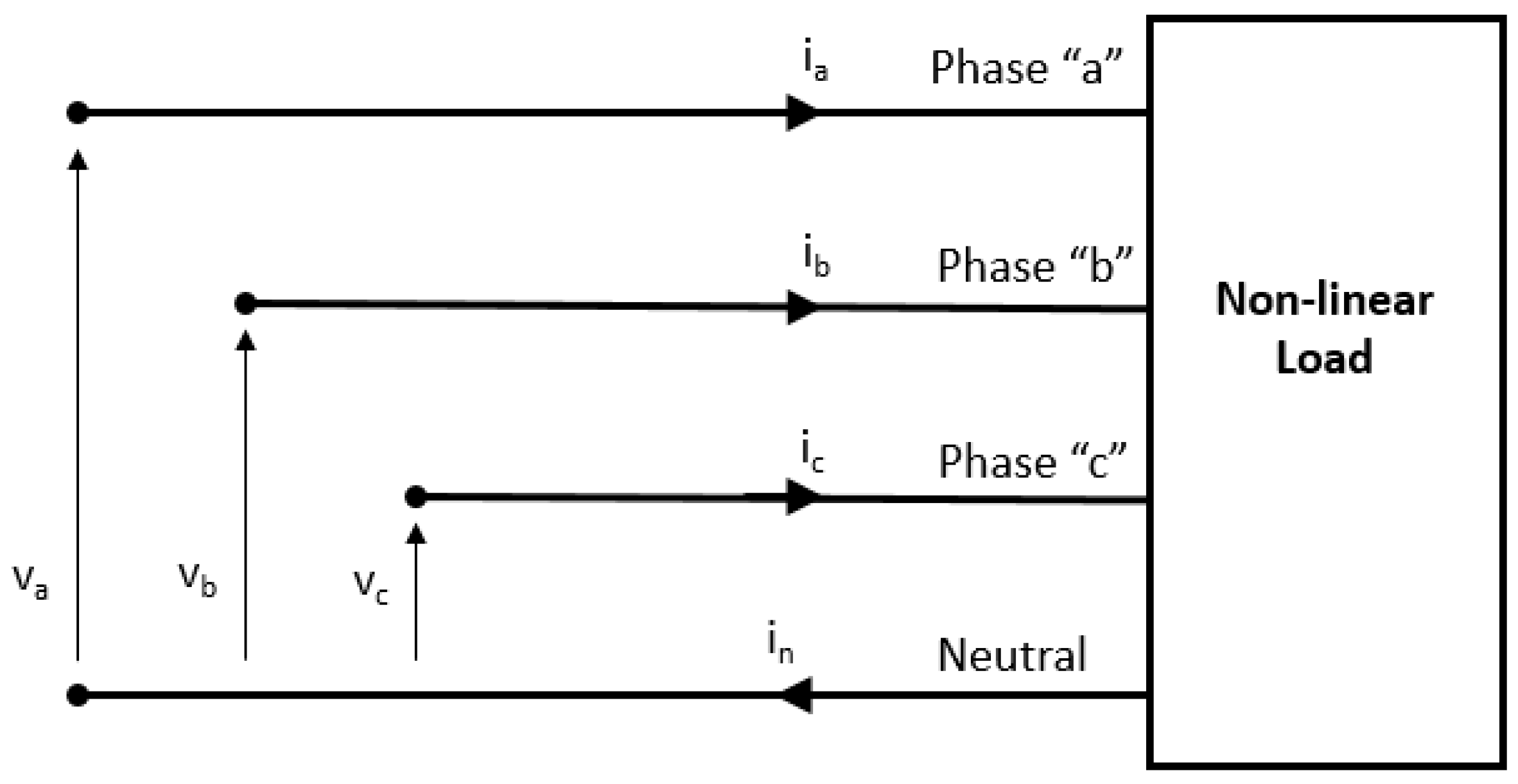
Figure 1 shows a non-linear load that is connected to an electrical system with non-sinusoidal balanced voltages.
where
where , and are line-to-neutral harmonic voltages of order m and , and are harmonic currents of order n.
These voltages can be expressed in terms of the following symmetrical components:
Similarly, the symmetric current components are
where
- and are the RMS values for the positive-sequence harmonic voltage and current of orders m and n, respectively.
- and are the RMS values for the negative-sequence harmonic voltage and current of orders m and n, respectively.
- and are the RMS values for the zero-sequence harmonic voltage and current of orders m and n, respectively.
- , and are, respectively, the angles of positive-, negative- and zero-sequence of the harmonic voltage of order m.
- , and are, respectively, the angles of positive-, negative- and zero-sequence of the harmonic current of order n.
As the voltages are balanced, the negative and zero-sequence voltages ( and ) become zero. The positive-sequence voltages for each phase (a, b and c) are determined as follows:
where .
Similarly, the phase-specific positive-, negative- and zero-sequence currents are
Under these conditions, the instantaneous power of the system is given by
where
Here,
- is the instantaneous power caused by positive-sequence voltages and currents.
- is the instantaneous power caused by positive-sequence voltages and negative-sequence currents.
- is the instantaneous power caused by positive-sequence voltages and zero-sequence currents.
Expressions of instantaneous power for voltage and current harmonics of order m and n, respectively, can then be obtained as
where
- is the angle between the positive-sequence harmonic voltage of order m and the positive-sequence harmonic current of order n.
- is the angle between the positive-sequence harmonic voltage of order m and the negative-sequence harmonic current of order n.
- is the angle between the positive-sequence harmonic voltage of order m and the zero-sequence harmonic current of order n.
Equation (23) can be decomposed into the following two terms:
where and are, respectively, the positive-sequence active power and the positive-sequence reactive power for a harmonic voltage of order m and a harmonic current of order n.
3.1. Harmonic Parameters , , and
A three-phase four-wire star-connected system with a single-phase load in the A-phase with balances and sinusoidal voltages will satisfy the following conditions:
Substituting these equalities into (24) and (25) produces the following expression:
If we proceed in this manner in connecting the load to Phase B and then to Phase C, applying the superposition theorem results in the following expression:
which can be decomposed into , , and as follows:
where
These instantaneous parameters are sinusoidal waveforms with zero average value and RMS values given by:
3.2. Phasor of Harmonic Apparent Power
For each harmonic voltage of order m ≠ 1 and harmonic current of order n ≠ 1, the phasor of harmonic apparent power can be defined as:
where
- , , and are the unit vectors associated with parameters , , and , respectively (see (35)–(38)).
- and are the unit vectors associated with the positive-sequence active power and the positive-sequence reactive power (see (26) and (27)).
As these unit vectors are all mutually orthogonal, the moduli of harmonic apparent power for a harmonic voltage of order m and harmonic current of order n is given by:
For m = n = 1, the phasor of fundamental apparent power is obtained as:
This expression is the same as that defined in [22]. In this phasor, the positive-sequence active and reactive power components, as well as the unbalanced power caused by unbalanced currents, are all included.
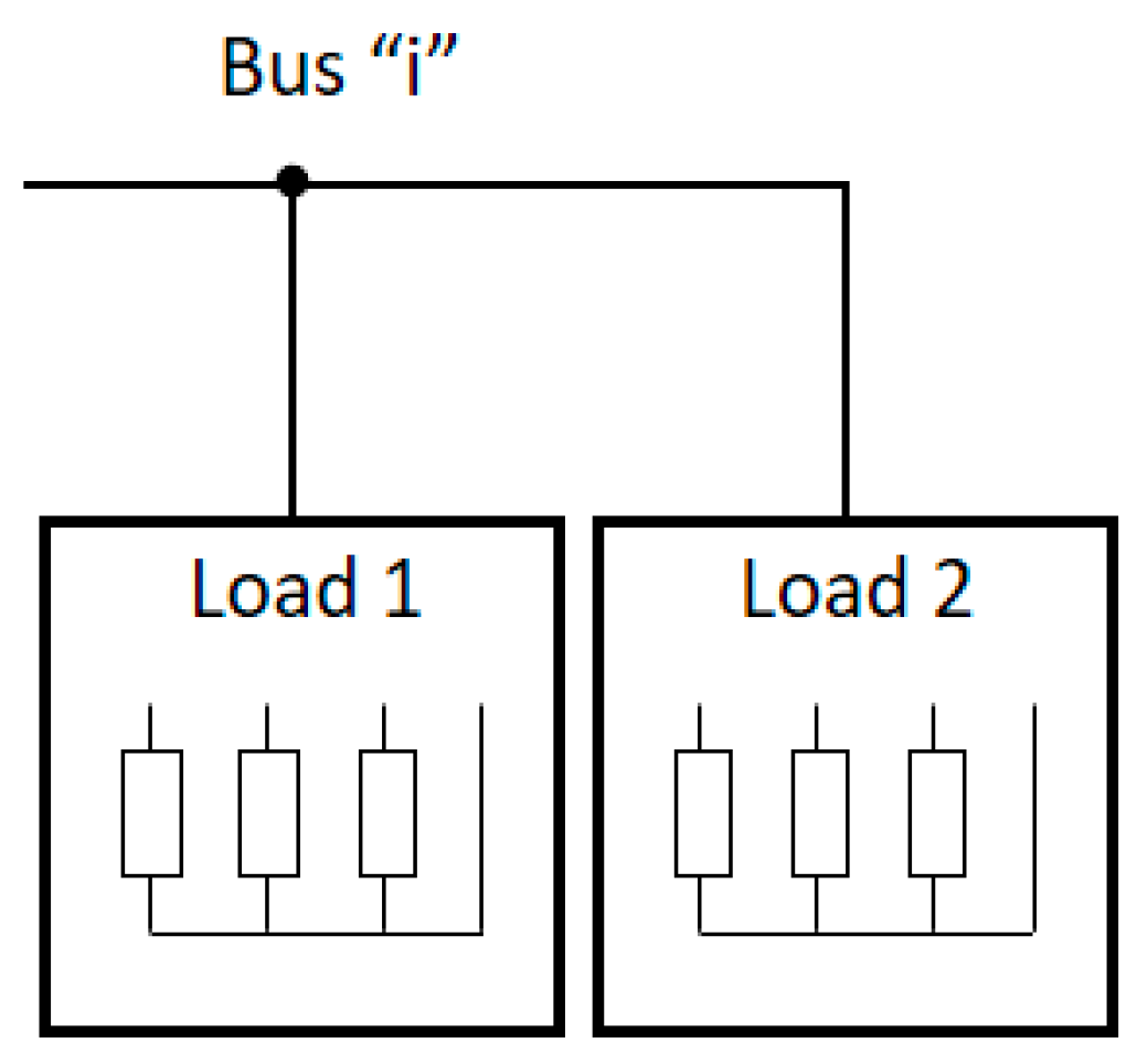
3.3. Application of on a Bus with Loads Connected in Parallel
Figure 2 shows two non-linear three-phase loads in a star configuration in which they are connected to bus ‘i’ of an electric power system.
Under these conditions, for a harmonic voltage of order m and harmonic current of order n, the phasor of harmonic apparent power in bus ‘i’ is given by the sum of the individual phasors of each load connected to the bus:
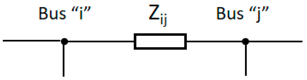
3.4. Application of between Two Buses in a System
Under these conditions, for a harmonic voltage of order m and harmonic current of order n the phasor of harmonic apparent power in the power line between the two buses is determined by subtracting the phasor in bus ‘j’ from that in bus ‘i’:
4. Harmonic Power in a Non-Linear Three-Phase Power System with Non-Sinusoidal Unbalanced Voltages
In Section 3, we assumed that the voltages were non-sinusoidal but balanced in each of the phases. In a real three-phase non-linear system, the voltages are normally both non-sinusoidal and unbalanced; in this case, the expression of the apparent power module defined by Buchholz in Reference [24] can be extended for voltage and current harmonics of order m and n, respectively, to obtain:
Substituting the voltage unbalance factors of order m, and , into (44) produces the following expression:
where and is referred to as the global harmonic voltage unbalance factor of order m. The expression under the second square root in (45) corresponds to the phasor magnitude apparent harmonic power defined in (39); this suggests that the modulus of the apparent power for a harmonic voltage of order m and a harmonic current of order n at any point of the system must be corrected and multiplied by as follows:
5. Total Harmonic Apparent Power and Total Apparent Power
In any node of a non-linear system, the number of harmonics of voltage and current that are considered will determine the number of phasors of harmonic apparent power. As these phasors are all mutually orthogonal, they do not sum arithmetically. In any node, the module of total harmonic apparent power is calculated from either of the following two expressions:
These values coincide with those obtained in IEEE Std. 1459-2010 [9] and by Buchholz [24]. Equation (47) or (48) can be alternatively expressed as a function of the fundamental harmonic of voltage and current (m = n = 1) in either of the two following manners:
where
The values and are, respectively, the rates of harmonic distortion of the currents and voltages of the three-phase system. Symmetrical components are determined by:
In terms of phase components, they are determined by:
At any point in the system, the module of total apparent power is given by:
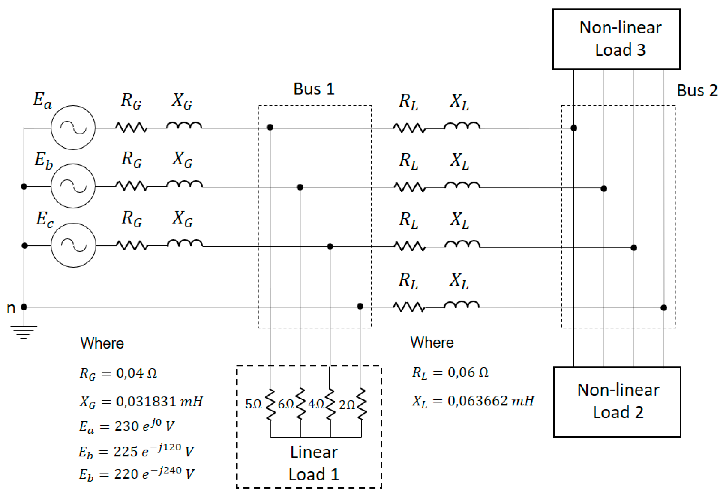
6. Practical Application
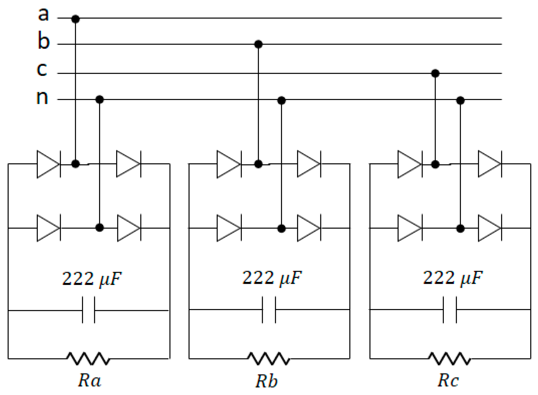
In this section, a practical case study for checking all of the concepts discussed in the previous sections is developed. Figure 4 shows a four-wire, two-bus electrical system with two unbalanced three-phase non-linear loads and an unbalanced three-phase linear load. All of the loads are modelled at a constant impedance. To simulate loads 2 and 3, we use single-phase full-wave rectifiers (see Figure 5). The values of Ra, Rb and Rc for loads 2 and 3 are listed in Table 1.
Using the ‘PSPICE’ analysis software (version 9.2), the harmonic line-to-neutral voltages in the buses (1 and 2) and harmonic currents circulating in the loads are obtained. These magnitudes are displayed in Table 2, Table 3 and Table 4. The harmonic currents supplied by the generator and the circulating currents along the line between buses 1 and 2 are easily deduced from the load currents. Here, we consider only harmonics 1, 3, 5 and 7 of voltage and current.
Table 5, Table 6, Table 7, Table 8, Table 9 and Table 10 list the results obtained using the equations formulated in the preceding sections, where:
- the values of and are calculated from (26), (27) and those of , , and are calculated from (35)–(38). The ‘line 1–2’ results in Table 10 are calculated from the difference between the corresponding node 1 and 2 values.
- the values of are calculated from (40).
Table 11 compares the following total apparent power values: (positive-sequence fundamental apparent power), which is calculated from and ; . (fundamental apparent power), which is calculated from (45); (total harmonic apparent power), which is calculated from (47); and (total apparent power), which is calculated from (55). These values are calculated from (48) and are the same as those obtained using IEEE Std. 1459–2010.
7. Conclusions
In a power system, there are several inefficient power components within the energy balance, and reducing or eliminating them requires that they be properly quantified. Three-phase sinusoidal systems are exclusively affected by fundamental voltage and current components, with imbalances in their magnitudes at fundamental frequencies leading to the appearance of unbalance power. This power component was analyzed by the authors in a previous work [22] through the application of the unbalance power phasor. In non-sinusoidal systems, the voltages and currents contain harmonic components other than the fundamental component that generate a harmonic power component that is also inefficient.
In this study, the authors extended the method they applied in analyzing unbalance power to the analysis of harmonic power by formulating the phasor of apparent harmonic power for the voltage harmonic of order ‘m’ and current harmonic of order ‘n’. The number of phasors depends on the number of voltage and current harmonics considered, and phasors of voltage and current harmonics of the same and different orders are considered. Each phasor of apparent harmonic power is formed from six parameters or components that are mutually orthogonal; these components are calculated from the harmonic voltages at the nodes of the network and from the circulating harmonic currents. For a node with several loads connected in parallel, the components of each resultant phasor are calculated as the arithmetic sum of the individual components of the loads. For nodes connected in serial, the components are calculated through arithmetic subtraction of the components. An expression of the modules of the total harmonic power and total apparent power at any point was also proposed. The results of these formulations were shown to coincide with those obtained using IEEE Std. 1459–2010.
The proposed set of phasors of harmonic power can be used in conjunction with the phasor of unbalance power to analyze all of the inefficient power components appearing in the transfer of energy in an electrical system, regardless of whether they are balanced or unbalanced or sinusoidal or non-sinusoidal. To validate the applicability of the proposed expressions and improve our understanding of them, we undertook practical case studies of four-wire systems with two nodes, unbalanced voltages and loads, and non-linear loads.
Author Contributions
Conceptualization, P.A.B., R.M. and J.M.D.; Methodology, P.A.B., R.M.-M., J.M.D. and R.M.; Validation, P.A.B., R.M.-M. and R.M.; Formal Analysis, P.A.B. and R.M.-M.; Investigation, P.A.B., R.M.-M., J.M.D. and R.M.; Resources, P.A.B. and R.M.-M.; Data Curation, P.A.B. and R.M.-M.; Writing—Original Draft Preparation, J.M.D. and R.M.; Writing—Review & Editing, R.M.-M., J.M.D. and R.M.; Visualization, P.A.B. and R.M.-M.; Supervision, J.M.D., R.M. and M.J.R.; Project Administration, J.M.D.
Funding
This work is supported by the Spanish Ministry of Economy and Competitiveness (MINECO) and the European Regional Development Fund (ERDF) under Grant ENE2015-64087-C2-2R.
Conflicts of Interest
The authors declare no conflict of interest.
References
- Emanuel, A.E. On the definition of power factor and apparent power in unbalanced polyphase circuits with sinusoidal voltage and currents. IEEE Trans. Power Deliv. 1993, 8, 841–852. [Google Scholar] [CrossRef]
- Jeon, S.J. Definitions of apparent power and power factor in a power system having transmission lines with unequal resistances. IEEE Trans. Power Deliv. 2005, 20, 1806–1811. [Google Scholar] [CrossRef]
- Jouane, A.V.; Banerjee, B. Assessment of voltage unbalance. IEEE Trans. Power Deliv. 2001, 16, 782–790. [Google Scholar] [CrossRef]
- Semlyen, A.; Acha, E.; Arrillaga, J. Newton-Type algorithms for the harmonic phasor analysis of nonlinear power circuits in periodical steady state with special reference to magnetic nonlinearities. IEEE Trans. Power Deliv. 1998, 3, 1090–1098. [Google Scholar] [CrossRef]
- Kersting, W.H. Causes and effects of unbalanced voltages serving an induction motor. IEEE Trans. Ind. Appl. 2001, 37, 165–170. [Google Scholar] [CrossRef]
- Wannous, K.; Toman, P. Evaluation of Harmonics Impact on Digital Relays. Energies 2018, 11, 893. [Google Scholar] [CrossRef]
- Viswanadha, G.K.; Bijwe, P.R. Efficient reconfiguration of balanced and unbalanced distribution systems for loss minimization. IET Gener. Transm. Distrib. 2008, 2, 7–12. [Google Scholar] [CrossRef]
- Pillay, P.; Manyage, M. Loss of life in induction machines operating with unbalanced supplies. IEEE Trans. Energy Convers. 2006, 21, 813–822. [Google Scholar] [CrossRef] [Green Version]
- Angarita, M.L.; Ramos, G.A. Power calculations in nonlinear and unbalanced conditions according to IEEE Std. 1459–2010. In Proceedings of the Power Electronics and Power Quality Applications (PEPQA), Bogota, Colombia, 6–7 July 2013; pp. 1–7. [Google Scholar] [CrossRef]
- IEEE Standards Association. IEEE Standard Definitions for the Measurement of Electric Power Quantities under Sinusoidal, Nonsinusoidal, Balanced, or Unbalanced Conditions, IEEE Std. 1459–2010; IEEE Standards Association: New York, NY, USA, 19 March 2010; pp. 1–50. [Google Scholar]
- Willems, J.L. Reflections on apparent power and power factor in non-sinusoidal and polyphase situations. IEEE Trans. Power Deliv. 2004, 19, 835–840. [Google Scholar] [CrossRef]
- Emanuel, A.E. Apparent powers definitions for three-phase systems. IEEE Trans. Power Deliv. 1999, 14, 767–772. [Google Scholar] [CrossRef]
- Chicco, G.; Schlabbach, J.; Spertino, F. Characterisation and assessment of the harmonic emission of grid-connected photovoltaic systems. In Proceedings of the 2005 IEEE Russia Power Tech, St. Petersburg, Russia, 27–30 June 2005; pp. 1–7. [Google Scholar] [CrossRef]
- Tan, Y.T.; Kirschen, D.S.; Jenkins, N. A model of PV generation suitable for stability analysis. IEEE Trans. Energy Convers. 2004, 19, 748–755. [Google Scholar] [CrossRef]
- Orchi, T.F.; Mahmud, M.A.; Oo, A.M.T. Generalized dynamical modeling of multiple photovoltaic units in a grid-connected system for analyzing dynamic interactions. Energies 2018, 11, 296. [Google Scholar] [CrossRef]
- Jayatunga, U.; Perera, S.; Ciufo, P.; Agalgaonkar, A.P. Deterministic methodologies for the quantification of voltage unbalance propagation in radial and interconnected networks. IET Gener. Transm. Distrib. 2015, 9, 1069–1076. [Google Scholar] [CrossRef] [Green Version]
- Bucci, G.; Ciancetta, F.; Fiorucci, E.; Ometto, A. Survey about classical and innovative definitions of the power quantities under nonsinusoidal conditions. Int. J. Emerg. Electr. Power Syst. 2017, 18, 1–16. [Google Scholar] [CrossRef]
- Barkas, D.A.; Psomopoulos, C.S.; Ioannidis, G.C.; Kaminaris, S.D.; Malatestas, P. Experimental and theoretical investigation of harmonic distortion in high voltage 3-phase transformers. In Proceedings of the MedPower 2014, Athens, Greece, 2–5 November 2014; pp. 1–8. [Google Scholar] [CrossRef]
- Marcos, B.K.; Cursino, B.J.; Lima, A.M.N. Shaping control strategies for active power filters. IET Power Electron. 2018, 11, 175–181. [Google Scholar] [CrossRef]
- Limongi, L.R.; Bradaschia, F.; de Oliveira Lima, C.H.; Cavalcanti, M.C. Reactive Power and Current Harmonic Control Using a Dual Hybrid Power Filter for Unbalanced Non-Linear Loads. Energies 2018, 11, 1392. [Google Scholar] [CrossRef]
- Xu, J.; Gu, X.; Liang, C.; Bai, Z.; Kubis, A. Harmonic suppression analysis of a harmonic filtering distribution transformer with integrated inductors based on field–circuit coupling simulation. IET Gener. Transm. Distrib. 2018, 12, 615–623. [Google Scholar] [CrossRef]
- Abdel Aleem, S.H.E.; Ibrahim, A.M.; Zobaa, A.F. Harmonic assessment-based adjusted current total harmonic distortion. J. Eng. 2016, 2016, 64–72. [Google Scholar] [CrossRef] [Green Version]
- Badr, M.; Maarouf, M.; Basyouni, M.M.; Ahmed, S.A. Reducing harmonic distortion and correcting power factor in distribution systems. In Proceedings of the 22nd International Conference and Exhibition on Electricity Distribution (CIRED 2013), Stockholm, Sweden, 10–13 June 2013; pp. 1–4. [Google Scholar] [CrossRef]
- Carvajal, W.; Ordoñez, G.; Moreno, A.L.; Duarte, C.A. Simulation of electric systems with non-linear and time-variant loads. Ingeniare Rev. Chilena Ing. 2011, 19, 76–92. [Google Scholar] [CrossRef]
- Sezgin, E.; Göl, M.; Salor, Ö. State-estimation-based determination of harmonic current contributions of iron and steel plants supplied from PCC. IEEE Trans. Ind. Appl. 2016, 52, 2654–2663. [Google Scholar] [CrossRef]
- Zebardast, A.; Mokhtari, H. Technique for online tracking of a utility harmonic impedance using by synchronising the measured samples. IET Gener. Transm. Distrib. 2016, 10, 1240–1247. [Google Scholar] [CrossRef]
- Ahmed, E.E.; Xu, W. Assessment of harmonic distortion level considering the interaction between distributed three-phase harmonic sources and power grid. IET Gener. Transm. Distrib. 2007, 1, 506–515. [Google Scholar] [CrossRef]
- Diez, J.M.; Blasco, P.A.; Montoya, R. Formulation of phasor unbalance power: Application to sinusoidal power systems. IET Gener. Transm. Distrib. 2016, 10, 4178–4186. [Google Scholar] [CrossRef]
- Montoya-Mira, R.; Diez, J.M.; Blasco, P.A.; Montoya, R. Equivalent circuit and calculation of unbalanced power in three-wire three-phase linear networks. IET Gener. Transm. Distrib. 2018, 12, 1466–1473. [Google Scholar] [CrossRef]
- Buchholz, F. Die drehstrom-scheinleistung bei ungleichmassiger belastung der drei zweige. Licht und Kraft 1922, 2, 9–11. [Google Scholar]
Figure 1.
Three-phase electrical system with non-linear load.

Figure 2.
Two parallel non-linear loads connected to a system bus.

Figure 3.
Two system buses linked by a power line.

Figure 4.
Three-phase electrical system with non-linear loads.

Figure 5.
Single-phase full-wave rectifier (loads 2 and 3).


Table 1.
Load 2 and 3 values (see Figure 5).
Table 1.
Load 2 and 3 values (see Figure 5).
| Resistance | Load 2 | Load 3 |
|---|---|---|
| Ra (Ω) | 7 | 5 |
| Rb (Ω) | 12 | 15 |
| Rc (Ω) | 20 | 25 |
Table 2.
Harmonic line-to-neutral voltage.
| Bus | Order | Vam (V) | Vbm (V) | Vcm (V) | |||
|---|---|---|---|---|---|---|---|
| m | Modulus | Angle | Modulus | Angle | Modulus | Angle | |
| Bus 1 | 1 | 227.5 | −0.086 | 223.0 | −120.1 | 217.6 | 119.9 |
| 3 | 0.261 | −137.4 | 0.188 | −127.1 | 0.14 | −121.1 | |
| 5 | 0.196 | −137.0 | 0.143 | −11.27 | 0.099 | 114.0 | |
| 7 | 0.174 | −137.6 | 0.126 | 108.2 | 0.085 | −5.423 | |
| Bus 2 | 1 | 226.4 | −0.109 | 222.2 | −120.1 | 217.0 | 119.9 |
| 3 | 0.704 | −131.9 | 0.521 | −122.4 | 0.376 | −115.9 | |
| 5 | 0.555 | −131.5 | 0.411 | −5.450 | 0.278 | 120.2 | |
| 7 | 0.507 | −133.0 | 0.375 | 112.0 | 0.248 | −1.351 | |
Table 3.
Harmonic currents in each phase and positive-sequence harmonic currents.
| Load | Order | Ian (A) | Ibn (A) | Icn (A) | In+ (A) | ||||
|---|---|---|---|---|---|---|---|---|---|
| n | Modulus | Angle | Modulus | Angle | Modulus | Angle | Modulus | Angle | |
| L1 | 1 | 45.59 | −3.68 | 39.1 | −118.5 | 51.51 | 121.4 | 45.36 | −0.271 |
| 3 | 0.032 | −143.2 | 0.013 | −124.8 | 0.01 | −98.12 | 0.008 | −144.7 | |
| 5 | 0.036 | −137.2 | 0.025 | −8.218 | 0.025 | 103.4 | 0.005 | −144.9 | |
| 7 | 0.033 | −138.8 | 0.208 | 102.1 | 0.024 | −3.652 | 0.088 | −136.7 | |
| L2 | 1 | 9.174 | −13.12 | 6.168 | −137.2 | 4.647 | 98.81 | 6.652 | −16.25 |
| 3 | 2.850 | 3.895 | 1.928 | 12.58 | 1.472 | 20.61 | 0.436 | 7.065 | |
| 5 | 1.679 | −9.547 | 1.113 | 117.2 | 0.823 | −116.6 | 0.266 | −41.31 | |
| 7 | 1.183 | −19.32 | 0.78 | −133.0 | 0.573 | 113.0 | 0.842 | −14.59 | |
| L3 | 1 | 7.435 | −15.47 | 5.363 | −139.5 | 4.197 | 96.69 | 5.656 | −18.68 |
| 3 | 2.297 | 7.58 | 1.678 | 15.97 | 1.337 | 23.77 | 0.312 | 8.613 | |
| 5 | 1.342 | −7.51 | 0.954 | 119.1 | 0.733 | −114.6 | 0.192 | −43.64 | |
| 7 | 0.946 | −18.04 | 0.667 | −131.8 | 0.509 | 114.3 | 0.704 | −13.12 | |
Table 4.
Harmonic line-to-neutral voltage in sequence components and voltages unbalance factors.
| Bus | Order | Vm+ (V) | Vm− (V) | Vm0 (V) | δm− | δm0 | |||
|---|---|---|---|---|---|---|---|---|---|
| m | Modulus | Angle | Modulus | Angle | Modulus | Angle | |||
| Bus 1 | 1 | 222.7 | −0.10 | 2.872 | 33.21 | 2.852 | −32.8 | 0.013 | 0.013 |
| 3 | 0.035 | −133.2 | 0.042 | −177.5 | 0.195 | −130.2 | 1.185 | 5.525 | |
| 5 | 0.030 | −174.9 | 0.145 | −132.6 | 0.028 | −121.0 | 4.778 | 0.910 | |
| 7 | 0.128 | −133.0 | 0.026 | −121.3 | 0.028 | −176.3 | 0.202 | 0.218 | |
| Bus 2 | 1 | 221.87 | −0.10 | 2.712 | 33.21 | 2.725 | −33.82 | 0.012 | 0.012 |
| 3 | 0.095 | −124.4 | 0.113 | −174.1 | 0.53 | −125.1 | 1.192 | 5.607 | |
| 5 | 0.088 | −171.1 | 0.413 | −126.9 | 0.079 | −114.6 | 4.692 | 0.894 | |
| 7 | 0.376 | −128.8 | 0.075 | −114.5 | 0.08 | −173.0 | 0.201 | 0.214 | |
Table 5.
Results in Bus 1.
| Harmonic | (VA) | (VA) | (VA) | (VA) | (W) | (VAr) | (VA) | ||
|---|---|---|---|---|---|---|---|---|---|
| m | n | ||||||||
| 1 | 1 | −2115.82 | −2638.24 | −138.238 | −1463.141 | 38,155.5 | 2534.16 | 0.018 | 38,423.27 |
| 1 | 3 | −2057.60 | −583.353 | 1460.40 | 188.710 | 490.788 | −64.749 | 0.018 | 2643.823 |
| 1 | 5 | −1240.00 | −70.671 | −820.267 | −79.911 | 223.934 | 207.223 | 0.018 | 1521.736 |
| 1 | 7 | −261.988 | −52.893 | −84.365 | −128.994 | 960.705 | 287.299 | 0.018 | 1049.309 |
| 3 | 1 | 0.297 | −0.080 | 0.423 | 0.263 | −3.843 | −4.702 | 5.650 | 35.010 |
| 3 | 3 | −0.123 | −0.237 | 0.233 | 0.211 | −0.061 | −0.050 | 5.650 | 2.409 |
| 3 | 5 | 0.094 | −0.132 | 0.147 | −0.091 | 0.000 | −0.048 | 5.650 | 1.387 |
| 3 | 7 | 0.003 | −0.014 | 0.043 | −0.018 | −0.071 | −0.143 | 5.650 | 0.956 |
| 5 | 1 | 0.330 | 0.306 | 0.027 | 0.224 | −5.158 | −0.817 | 4.864 | 26.051 |
| 5 | 3 | 0.289 | 0.009 | −0.202 | 0.037 | −0.068 | 0.003 | 4.864 | 1.793 |
| 5 | 5 | 0.168 | −0.011 | 0.114 | 0.006 | −0.028 | −0.031 | 4.864 | 1.032 |
| 5 | 7 | 0.032 | −0.012 | 0.016 | 0.018 | −0.127 | −0.051 | 4.864 | 0.711 |
| 7 | 1 | 1.072 | −0.291 | 1.535 | 0.947 | −13.864 | −17.045 | 0.297 | 23.027 |
| 7 | 3 | −0.449 | −0.854 | 0.849 | 0.757 | −0.219 | −0.181 | 0.297 | 1.584 |
| 7 | 5 | 0.339 | −0.477 | 0.530 | −0.330 | 0.000 | −0.175 | 0.297 | 0.912 |
| 7 | 7 | 0.011 | 0.049 | 0.156 | −0.067 | −0.255 | −0.517 | 0.297 | 0.629 |
Table 6.
Results in Bus 2.
| Harmonic | (VA) | (VA) | (VA) | (VA) | (W) | (VAr) | (VA) | ||
|---|---|---|---|---|---|---|---|---|---|
| m | n | ||||||||
| 1 | 1 | −2052.78 | 742.814 | −72.357 | −181.155 | 7821.842 | 2430.956 | 0.017 | 8480.335 |
| 1 | 3 | −2058.52 | −587.648 | 1456.722 | 195.425 | 493.339 | −67.699 | 0.017 | 2644.456 |
| 1 | 5 | −1246.02 | −61.539 | −825.547 | −69.403 | 225.739 | 204.571 | 0.017 | 1528.464 |
| 1 | 7 | −242.657 | −91.012 | −51.341 | −146.629 | 999.69 | 245.924 | 0.017 | 1073.082 |
| 3 | 1 | −0.299 | −0.343 | 0.611 | −0.54 | −1.02 | −3.337 | 5.732 | 21.022 |
| 3 | 3 | −0.552 | −0.387 | 0.835 | 0.27 | −0.142 | −0.157 | 5.732 | 6.555 |
| 3 | 5 | 0.184 | −0.367 | 0.359 | −0.331 | 0.018 | −0.129 | 5.732 | 3.789 |
| 3 | 7 | −0.006 | −0.005 | 0.096 | −0.085 | −0.153 | −0.411 | 5.732 | 2.66 |
| 5 | 1 | 0.666 | −0.518 | 0.132 | 0.166 | −2.916 | −1.439 | 4.777 | 16.426 |
| 5 | 3 | 0.822 | −0.12 | −0.562 | 0.236 | −0.198 | −0.004 | 4.777 | 5.122 |
| 5 | 5 | 0.484 | −0.078 | 0.336 | 0.001 | −0.076 | −0.094 | 4.777 | 2.961 |
| 5 | 7 | 0.072 | −0.057 | 0.047 | 0.061 | −0.377 | −0.158 | 4.777 | 2.078 |
| 7 | 1 | −1.096 | −1.735 | 2.602 | −1.667 | −5.063 | −12.905 | 0.293 | 14.954 |
| 7 | 3 | −1.804 | −2.092 | 2.959 | 1.712 | −0.611 | −0.58 | 0.293 | 4.663 |
| 7 | 5 | 0.86 | −1.449 | 1.505 | −1.149 | 0.031 | −0.515 | 0.293 | 2.695 |
| 7 | 7 | −0.042 | −0.055 | 0.426 | −0.274 | −0.733 | −1.581 | 0.293 | 1.892 |
Table 7.
Results in load 1.
| Harmonic | (VA) | (VA) | (VA) | (VA) | (W) | (VAr) | (VA) | ||
|---|---|---|---|---|---|---|---|---|---|
| m | n | ||||||||
| 1 | 1 | −55.554 | −3384.39 | −65.46 | −1281.05 | 30,304.59 | 93.023 | 0.018 | 30,525.2 |
| 1 | 3 | 8.837 | 5.75 | −1.922 | −6.779 | −4.413 | 3.137 | 0.018 | 13.791 |
| 1 | 5 | 10.703 | −9.126 | 8.391 | −10.302 | −2.625 | 1.853 | 0.018 | 19.617 |
| 1 | 7 | −18.464 | 38.519 | −32.779 | 18.204 | −42.707 | 40.317 | 0.018 | 81.743 |
| 3 | 1 | 0.383 | 0.117 | 0.171 | 0.375 | −3.275 | −3.527 | 5.65 | 27.813 |
| 3 | 3 | 0 | 0.002 | 0 | −0.001 | 0.001 | 0 | 5.65 | 0.013 |
| 3 | 5 | 0 | 0.002 | 0 | 0.002 | 0 | 0 | 5.65 | 0.018 |
| 3 | 7 | 0.008 | −0.005 | 0 | 0.001 | 0.009 | 0.001 | 5.65 | 0.074 |
| 5 | 1 | 0.075 | 0.455 | −0.001 | 0.178 | −4.12 | −0.388 | 4.864 | 20.696 |
| 5 | 3 | −0.001 | −0.001 | 0 | 0.001 | 0.001 | 0 | 4.864 | 0.009 |
| 5 | 5 | −0.001 | 0.001 | −0.001 | 0.001 | 0 | 0 | 4.864 | 0.013 |
| 5 | 7 | 0.004 | 0.005 | 0.004 | −0.003 | 0.006 | −0.005 | 4.864 | 0.055 |
| 7 | 1 | 1.386 | 0.418 | 0.624 | 1.357 | −11.819 | −12.786 | 0.297 | 18.293 |
| 7 | 3 | −0.001 | 0.006 | −0.001 | −0.003 | 0.003 | 0.001 | 0.297 | 0.008 |
| 7 | 5 | 0.001 | 0.008 | 0 | 0.007 | 0.002 | 0 | 0.297 | 0.012 |
| 7 | 7 | 0.028 | −0.017 | 0.001 | 0.003 | 0.034 | 0.002 | 0.297 | 0.049 |
Table 8.
Results in load 2.
| Harmonic | (VA) | (VA) | (VA) | (VA) | (W) | (VAr) | (VA) | ||
|---|---|---|---|---|---|---|---|---|---|
| m | n | ||||||||
| 1 | 1 | −1200.93 | 419.477 | −38.06 | −101.712 | 4253.073 | 1231.714 | 0.017 | 4608.92 |
| 1 | 3 | −1133.33 | −294.699 | 779.618 | 70.706 | 288.081 | −36.232 | 0.017 | 1438.41 |
| 1 | 5 | −685.076 | −42.472 | −440.704 | −48.682 | 133.342 | 116.764 | 0.017 | 836.27 |
| 1 | 7 | −142.086 | −51.436 | −28.3 | −84.158 | 542.853 | 140.298 | 0.017 | 587.532 |
| 3 | 1 | −0.174 | −0.203 | 0.359 | −0.31 | −0.586 | −1.793 | 5.732 | 11.425 |
| 3 | 3 | −0.298 | −0.202 | 0.462 | 0.131 | −0.082 | −0.093 | 5.732 | 3.566 |
| 3 | 5 | 0.1 | −0.198 | 0.202 | −0.177 | 0.009 | −0.075 | 5.732 | 2.073 |
| 3 | 7 | −0.004 | −0.003 | 0.056 | −0.049 | −0.081 | −0.225 | 5.732 | 1.456 |
| 5 | 1 | 0.392 | −0.298 | 0.074 | 0.096 | −1.591 | −0.747 | 4.777 | 8.927 |
| 5 | 3 | 0.448 | −0.075 | −0.295 | 0.141 | −0.115 | −0.004 | 4.777 | 2.786 |
| 5 | 5 | 0.266 | −0.04 | 0.181 | 0.006 | −0.045 | −0.054 | 4.777 | 1.62 |
| 5 | 7 | 0.042 | −0.033 | 0.027 | 0.035 | −0.204 | −0.089 | 4.777 | 1.138 |
| 7 | 1 | −0.632 | −1.023 | 1.523 | −0.95 | −2.872 | −6.922 | 0.293 | 8.127 |
| 7 | 3 | −0.983 | −1.104 | 1.653 | 0.874 | −0.353 | −0.342 | 0.293 | 2.536 |
| 7 | 5 | 0.468 | −0.782 | 0.8438 | −0.6093 | 0.0132 | −0.2997 | 0.293 | 1.47 |
| 7 | 7 | −0.025 | −0.034 | 0.2487 | −0.156 | −0.3889 | −0.8656 | 0.293 | 1.04 |
Table 9.
Results in load 3.
| Harmonic | (VA) | (VA) | (VA) | (VA) | (W) | (VAr) | (VA) | ||
|---|---|---|---|---|---|---|---|---|---|
| m | n | ||||||||
| 1 | 1 | −851.848 | 323.337 | −34.297 | −79.444 | 3568.768 | 1199.2412 | 0.017 | 3875.11 |
| 1 | 3 | −925.192 | −292.949 | 677.104 | 124.719 | 205.258 | −31.467 | 0.017 | 1208.05 |
| 1 | 5 | −560.943 | −19.067 | −384.842 | −20.720 | 92.3965 | 87.8068 | 0.017 | 692.781 |
| 1 | 7 | −100.571 | −39.576 | −23.041 | −62.471 | 456.837 | 105.625 | 0.017 | 485.841 |
| 3 | 1 | −0.125 | −0.140 | 0.252 | −0.230 | −0.4337 | −1.5443 | 5.732 | 9.606 |
| 3 | 3 | −0.254 | −0.186 | 0.373 | 0.139 | −0.0603 | −0.0647 | 5.732 | 2.995 |
| 3 | 5 | 0.084 | −0.170 | 0.157 | −0.154 | 0.0088 | −0.0536 | 5.732 | 1.717 |
| 3 | 7 | −0.002 | −0.001 | 0.040 | −0.037 | −0.0724 | −0.1862 | 5.732 | 1.204 |
| 5 | 1 | 0.274 | −0.220 | 0.058 | 0.070 | −1.3247 | −0.6917 | 4.777 | 7.506 |
| 5 | 3 | 0.375 | −0.045 | −0.267 | 0.096 | −0.0824 | −0.0004 | 4.777 | 2.340 |
| 5 | 5 | 0.218 | −0.038 | 0.156 | −0.005 | −0.0308 | −0.0402 | 4.777 | 1.342 |
| 5 | 7 | 0.029 | −0.024 | 0.020 | 0.026 | −0.1726 | −0.07 | 4.777 | 0.941 |
| 7 | 1 | −0.095 | −0.067 | 0.161 | −0.233 | −0.2011 | −1.2414 | 0.293 | 6.531 |
| 7 | 3 | −0.230 | −0.062 | 0.318 | 0.015 | −0.0413 | −0.056 | 0.293 | 2.036 |
| 7 | 5 | 0.050 | −0.133 | 0.109 | −0.140 | 0.0116 | −0.0410 | 0.293 | 1.168 |
| 7 | 7 | 0.002 | 0.002 | 0.024 | −0.035 | −0.0399 | −0.1515 | 0.293 | 0.819 |
Table 10.
Results in line 1–2 (Bus 1–Bus 2).
| Harmonic | (VA) | (VA) | (VA) | (VA) | (W) | (VAr) | (VA) | ||
|---|---|---|---|---|---|---|---|---|---|
| m | n | ||||||||
| 1 | 1 | −7.467 | 3.324 | −0.44 | −0.928 | 29.051 | 10.185 | 0.252 | 32.861 |
| 1 | 3 | −7.882 | −1.45 | 5.569 | 0.058 | 1.862 | −0.188 | 0.252 | 10.247 |
| 1 | 5 | −4.683 | −0.007 | −3.115 | −0.206 | 0.82 | 0.799 | 0.252 | 5.923 |
| 1 | 7 | −0.865 | −0.398 | −0.246 | −0.567 | 3.722 | 1.058 | 0.252 | 4.158 |
| 3 | 1 | 0.188 | 0.15 | −0.334 | 0.424 | 0.452 | 2.162 | 5.739 | 13.318 |
| 3 | 3 | 0.393 | 0.128 | −0.564 | −0.037 | 0.081 | 0.107 | 5.739 | 4.153 |
| 3 | 5 | −0.095 | 0.232 | −0.208 | 0.239 | −0.019 | 0.08 | 5.739 | 2.4 |
| 3 | 7 | −0.002 | −0.002 | −0.05 | 0.064 | 0.073 | 0.268 | 5.739 | 1.685 |
| 5 | 1 | −0.408 | 0.366 | −0.107 | −0.117 | 1.878 | 1.009 | 4.742 | 10.699 |
| 5 | 3 | −0.526 | 0.128 | 0.353 | −0.199 | 0.129 | 0.007 | 4.742 | 3.336 |
| 5 | 5 | −0.313 | 0.065 | −0.223 | 0.004 | 0.048 | 0.063 | 4.742 | 1.928 |
| 5 | 7 | −0.043 | 0.04 | −0.035 | −0.039 | 0.243 | 0.112 | 4.742 | 1.354 |
| 7 | 1 | 0.762 | 1.025 | −1.671 | 1.259 | 3.018 | 8.647 | 0.291 | 9.875 |
| 7 | 3 | 1.33 | 1.209 | −2.082 | −0.929 | 0.389 | 0.398 | 0.291 | 3.079 |
| 7 | 5 | −0.525 | 0.962 | −0.971 | 0.813 | −0.034 | 0.339 | 0.291 | 1.78 |
| 7 | 7 | 0.022 | 0.024 | −0.268 | 0.203 | 0.444 | 1.062 | 0.291 | 1.25 |
Table 11.
Summary of apparent power components.
| ID | ||||
|---|---|---|---|---|
| Bus 1 | 38,239.55 | 38,423.268 | 3328.831 | 38,567.196 |
| Bus 2 | 8190.894 | 8480.335 | 3339.87 | 9114.319 |
| Load 1 | 30,304.737 | 30,525.191 | 95.775 | 30,525.341 |
| Load 2 | 4427.839 | 4608.918 | 1820.784 | 4955.54 |
| Load 3 | 3764.875 | 3875.109 | 1521.095 | 4162.956 |
| Line 1–2 | 30.785 | 32.861 | 26.84 | 42.429 |
© 2018 by the authors. Licensee MDPI, Basel, Switzerland. This article is an open access article distributed under the terms and conditions of the Creative Commons Attribution (CC BY) license (http://creativecommons.org/licenses/by/4.0/).
Share and Cite
MDPI and ACS Style
Blasco, P.A.; Montoya-Mira, R.; Diez, J.M.; Montoya, R.; Reig, M.J. Formulation of the Phasors of Apparent Harmonic Power: Application to Non-Sinusoidal Three-Phase Power Systems. Energies 2018, 11, 1888. https://doi.org/10.3390/en11071888
AMA Style
Blasco PA, Montoya-Mira R, Diez JM, Montoya R, Reig MJ. Formulation of the Phasors of Apparent Harmonic Power: Application to Non-Sinusoidal Three-Phase Power Systems. Energies. 2018; 11(7):1888. https://doi.org/10.3390/en11071888
Chicago/Turabian StyleBlasco, Pedro A., Rafael Montoya-Mira, José M. Diez, Rafael Montoya, and Miguel J. Reig. 2018. "Formulation of the Phasors of Apparent Harmonic Power: Application to Non-Sinusoidal Three-Phase Power Systems" Energies 11, no. 7: 1888. https://doi.org/10.3390/en11071888
Note that from the first issue of 2016, this journal uses article numbers instead of page numbers. See further details here.