Adaptive Control Method of Sensorless Permanent Magnet Synchronous Motor Based on Super-Twisting Sliding Mode Algorithm

Abstract

To solve the problem of the sensorless control method of a permanent magnet synchronous motor, based on the study of a mathematical model for a permanent magnet synchronous motor and model adaptation theory, a reference model equation and adjustable model equation are derived according to the stator current equation. The correctness of the selected linear compensator matrix is strictly proved. Then, Popov’s super-stability theory is used to derive the speed adaptive law and prove its asymptotic stability. Based on the voltage closed-loop feedback MTPA weak magnetic control strategy, a simulation model of a MRAS control system based on stator current is built and combined with the principle of MRAS. Aiming to investigate the problem that the PI adaptive law in the traditional MRAS algorithm is not robust, super-twisting sliding mode control is introduced to replace the PI adaptive law. The observer based on STSM−MRAS is designed. The simulation model of the MRAS control system based on the super-twisting sliding mode is established. Under certain working conditions, the STSM−MRAS algorithm and the traditional MRAS algorithm are simulated and compared. The results show that the STSM−MRAS algorithm can improve the steady-state performance and robustness of a sensorless control system.

1. Introduction

Permanent magnet synchronous machines (PMSM) are widely used in various industries due to their high power density and reliable performance [1]. Especially in the field of new energy [2,3], PMSMs are widely used because of their low environmental pollution [4]. PMSMs are more stable than DC motors in performance and are more efficient than asynchronous motors [5]. Therefore, in order to improve the performance of PMSMs, more advanced control technologies should be adopted [6]. The model reference adaptive system (MRAS) takes the motor body as the reference model, the stator current equation is taken as an adjustable model, and the estimated speed is taken as an adjustable parameter [7]. The parameters such as the estimated speed can be obtained by calculating the difference between the actual parameters and the estimated parameters, and then inputting the error into the PI regulator [8,9]. However, because the traditional MRAS algorithm is not robust, when the motor load is disturbed, the estimation accuracy of the MRAS algorithm will be affected [10]. Therefore, the sliding mode control is introduced to replace the PI adaptive law in the MRAS algorithm [11,12], which improves its robustness [13,14].

In [15], a novel switching linear feedback sliding mode controller (SLF-SMC) design method is proposed. Simulation and implementation studies under different operating conditions, such as speed range and inertia variation, show that the dynamic performance of sensorless field orientation control (SFOC) with MRAS-SMC is higher than that with MRAS-PI. In [16], two types of speed, torque and flux estimators are introduced. A sliding mode observer (SMO) and a model reference adaptive system (MRAS) type estimator are applied to sensorless direct torque control of a space vector modulation algorithm (DTC-SVM) driven by an induction motor (IM). This solves the problem of obtaining motor parameters without sensors. In [17], a new predictive model reference adaptive system (MRAS) velocity estimator is proposed. This eliminates the proportional integral (PI) controller used in the adaptive mechanism of the traditional MRAS estimator. In [18], a novel predictive MRAS rotor velocity estimator for sensorless IM drive is proposed. Compared with the traditional PI controller, this estimator improves the algorithm and reduces the computation.

This paper first studies the principle and basic structure of MRAS. The reference model equation and adjustable model equation are derived according to the stator current equation [19,20,21,22]. Based on Popov’s super-stability theory, a speed adaptive law is designed and its asymptotic stability is proved. The simulation experiments under different working conditions were carried out on the Matlab/Simulink platform. The feasibility and accuracy of the MRAS algorithm are verified [23]. In order to solve the problem that the PI adaptive law in the traditional MRAS algorithm is not robust [24], super-twisting sliding mode control is introduced to replace the PI adaptive law [25]. The super-twisting sliding mode MRAS observer is designed and its stability is analyzed. Under certain working conditions, the super-twisting sliding mode MRAS algorithm and the traditional MRAS algorithm are simulated and compared [26].

2. Mathematical Model of PMSM

The stator voltage equation of PMSM in the two-phase rotating coordinate system is [27]:

$$\{\begin{array}{l}{u}_d=R{i}_d+L_d\frac{\mathrm{d}}{\mathrm{d}t}{i}_d-{\omega }_e{L}_q{i}_q\\ u_q=R{i}_q+L_q\frac{\mathrm{d}}{\mathrm{d}t}{i}_q+{\omega }_e\left(L_d{i}_d+{\psi }_f\right)\end{array}$$

(1)

$u_d$ and $u_q$ are the direct and quadrature components of space voltage vector. $i_d$ and $i_q$ are the direct and quadrature components of space current vector. ${\psi }_d$ and ${\psi }_q$ are the direct and quadrature components of space flux vector. $R$ is the phase resistance of the stator winding and ${\omega }_e$ is the electrical angular velocity.

The direct axis and cross axis components of the flux are [28]:

$$\{\begin{array}{l}{\psi }_d=L_d{i}_d+{\psi }_f\\ {\psi }_q=L_q{i}_q\end{array}$$

(2)

$L_d$ and $L_q$ are direct axis and quadrature axis synchronization inductors; ${\psi }_f$ is the magnetic field of the fundamental wave excited by the permanent magnet. The voltage equivalent circuit in the synchronous rotating coordinate system d-q can be obtained [29], as shown in Figure 1.

The electromagnetic torque equation and the motion equation under the synchronous rotating coordinate system d-q are:

$$T_e=\frac{3}{2}{p}_{\mathrm{n}}{i}_q\left[i_d\left(L_d-L_q\right)+{\psi }_f\right]$$

(3)

$$\frac{J}{p_{\mathrm{n}}}\frac{\mathrm{d}}{\mathrm{d}t}{\omega }_e=T_e-T_{\mathrm{L}}-\frac{B}{p_{\mathrm{n}}}{\omega }_e$$

(4)

3. MRAS Based on Stator Current

The identification idea of MRAS is to take the parameters to be identified as adjustable parameters [30]. The expression containing parameters to be identified is regarded as the adjustable model, and the expression without unknown parameters is regarded as the reference model. We want the physical meaning of x and $\widehat{x}$ to be the same. Subtract $\widehat{x}$ from x to get the generalized error e. The suitable adaptive law is designed to adjust the parameters to be identified in the tunable model, so that the generalized error e can approach zero. In this way, the output of the system is asymptotically stable, and the accurate identification of system parameters is finally realized. The parallel type MRAS is widely used, and the parallel type structure is selected as the research object in this paper. Figure 2 shows the structure diagram of the parallel type.

3.1. Reference Model and Adjustable Model

For the PMSM, the current equation in the synchronous rotating coordinate system is [31]:

$$\{\begin{array}{l}\frac{\mathrm{d}}{\mathrm{d}t}{i}_d=-\frac{R}{L_{\mathrm{d}}}{i}_d+{\omega }_e\frac{L_q}{L_d}{i}_q+\frac{1}{L_d}{u}_d\\ \frac{\mathrm{d}}{\mathrm{d}t}{i}_q=-\frac{R}{L_q}{i}_q-{\omega }_e\frac{L_d}{L_q}{i}_d-\frac{{\psi }_f}{L_q}{\omega }_e+\frac{1}{L_q}{u}_q\end{array}$$

(5)

To obtain the adjustable model, change the above formula to:

$$\{\begin{array}{l}\frac{\mathrm{d}}{\mathrm{d}t}(i_d+\frac{{\psi }_f}{L_d})=-\frac{R}{L_d}(i_d+\frac{{\psi }_f}{L_d})+{\omega }_e\frac{L_q}{L_d}{i}_q+\frac{1}{L_d}(u_d+\frac{R}{L_d}{\psi }_f)\\ \frac{\mathrm{d}}{\mathrm{d}t}{i}_q=-\frac{R}{L_q}{i}_q-{\omega }_e\frac{L_d}{L_q}(i_d+\frac{{\psi }_f}{L_d})+\frac{1}{L_q}{u}_q\end{array}$$

(6)

$$\{\begin{array}{l}{i^{\prime }}_d=i_d+\frac{{\psi }_f}{L_d}\\ {i^{\prime }}_q=i_q\\ {u^{\prime }}_d=u_d+\frac{R}{L_d}{\psi }_f\\ {u^{\prime }}_q=u_q\end{array}$$

(7)

Equation (7) is written as a space state expression of the form:

$$\frac{\mathrm{d}}{\mathrm{d}t}{i}^{\prime }=A{i}^{\prime }+B{u}^{\prime }$$

(8)

$$i^{\prime }=\left[\begin{array}{c}{i^{\prime }}_d\\ {i^{\prime }}_q\end{array}\right],u^{\prime }=\left[\begin{array}{c}{u^{\prime }}_d\\ {u^{\prime }}_q\end{array}\right],A=\left[\begin{array}{cc}-\frac{R}{L_d}& {\omega }_e\frac{L_q}{L_d}\\ -{\omega }_e\frac{L_d}{L_q}& -\frac{R}{L_q}\end{array}\right],B=\left[\begin{array}{cc}\frac{1}{L_d}& 0\\ 0& \frac{1}{L_q}\end{array}\right]$$

When (8) is expressed as an estimated value, we can obtain:

$$\frac{\mathrm{d}}{\mathrm{d}t}\widehat{i^{\prime }}=\widehat{A}\widehat{i^{\prime }}+B{u}^{\prime }$$

(9)

$$\widehat{i^{\prime }}=\left[\begin{array}{c}{\widehat{i^{\prime }}}_d\\ {\widehat{i^{\prime }}}_q\end{array}\right],\widehat{A}=\left[\begin{array}{cc}-\frac{R}{L_d}& {\widehat{\omega }}_e\frac{L_q}{L_d}\\ -{\widehat{\omega }}_e\frac{L_d}{L_q}& -\frac{R}{L_q}\end{array}\right]$$

Since matrix $A$ and $\widehat{A}$ contains rotor speed information, Equation (9) can be used as an adjustable model, Equation (5) as a reference model, and ω_e as an adjustable parameter.

3.2. Design of Reference Adaptive Law

By defining the generalized error $e=i^{\prime }-\widehat{i^{\prime }}$ and subtracting Equations (8) and (9), we can get:

$$\frac{\mathrm{d}}{\mathrm{d}t}\left[\begin{array}{c}{e}_d\\ e_q\end{array}\right]=\left[\begin{array}{cc}-\frac{R}{L_d}& {\omega }_e\frac{L_q}{L_d}\\ -{\omega }_e\frac{L_d}{L_q}& -\frac{R}{L_q}\end{array}\right]\left[\begin{array}{c}{e}_d\\ e_q\end{array}\right]-J({\widehat{\omega }}_e-{\omega }_e)\left[\begin{array}{c}{\widehat{i^{\prime }}}_d\\ {\widehat{i^{\prime }}}_q\end{array}\right]$$

(10)

$$e_d={i^{\prime }}_d-{\widehat{i^{\prime }}}_d,e_q={i^{\prime }}_q-{\widehat{i^{\prime }}}_q,J=\left[\begin{array}{cc}0& \frac{L_q}{L_d}\\ -\frac{L_d}{L_q}& 0\end{array}\right]$$

$$\frac{\mathrm{d}}{\mathrm{d}t}e=Ae-W$$

(11)

Equation (11) can be written as an equation of state:

$$\{\begin{array}{c}\dot{e}=Ae-W\\ V=Ce\end{array}$$

(12)

Figure 3 shows a standard feedback system obtained according to Equation (12). In the figure, the matrix C is a linear compensator, and the forward channel in the dashed box in the upper half is a linear time-invariant system. Since the relationship between output V and feedback W cannot be completely determined, it can be represented by a nonlinear time-varying feedback channel [32], as shown in the dashed box at the bottom of Figure 3.

According to Popov’s super-stability theory, the following two conditions must be met to make the system asymptotically stable [33]:

1.

Transfer function matrix $G(s)=C{(sI-A)}^{-1}$ of linear time-invariant forward channel is strictly positive real matrix;

2.

The nonlinear time-varying feedback channel satisfies Popov’s integral inequality and ${\gamma }_0^2$ is any finite positive number.

$$\eta (0,t_1)={\displaystyle {\int }_0^{t_1}{V}^{\mathrm{T}}W\mathrm{d}t\ge }-{\gamma }_0^2\begin{array}{cc}& (\forall t_1\ge 0)\end{array}$$

(13)

$$\{\begin{array}{c}\dot{x}(t)=Ax(t)+Bu(t)\\ y(t)=Cx(t)+Du(t)\end{array}$$

(14)

According to the positive real lemma, the necessary and sufficient condition for the transfer function matrix A of the state equation of linear time-invariant system to be $G(s)=D+C{(sI-A)}^{-1}B$ strictly positive real matrix is the existence of symmetric positive definite matrix P and real matrix K, L, positive real number $\lambda$, or symmetric positive definite matrix Q which satisfies the condition:

$$\{\begin{array}{c}\dot{x}(t)=Ax(t)+Bu(t)\\ y(t)=Cx(t)+Du(t)\end{array}$$

(15)

Since B = I and D = 0, Equation (15) can be reduced to:

$$\{\begin{array}{l}PA+A^{\mathrm{T}}P=-Q\\ P=C\end{array}$$

(16)

Firstly, C is taken as the identity matrix. According to Equation (16), matrix P and matrix A are equal and symmetric positive definite matrices. Then, matrix A and matrix P are substituted into Equation (16) to obtain:

$$Q=-(PA+A^{\mathrm{T}}P)=\left[\begin{array}{cc}2\frac{R}{L_d}& {\omega }_e(\frac{L_d}{L_q}-\frac{L_q}{L_d})\\ {\omega }_e(\frac{L_d}{L_q}-\frac{L_q}{L_d})& 2\frac{R}{L_q}\end{array}\right]$$

(17)

Therefore, the first order major subequation of matrix Q is $2\frac{R}{L_d}>0$, and the second order major subequation of matrix Q is:

$$\begin{array}{ll}\left|Q\right|& =\frac{4R^2}{L_d{L}_q}-{\omega }_e^2{\left(\frac{L_d^2-L_q^2}{L_d{L}_q}\right)}^2\\ & =\left(\frac{2R}{\sqrt{L_d{L}_q}}+{\omega }_e\frac{\left|L_d^2-L_q^2\right|}{L_d{L}_q}\right)\left(\frac{2R}{\sqrt{L_d{L}_q}}-{\omega }_e\frac{\left|L_d^2-L_q^2\right|}{L_d{L}_q}\right)\end{array}$$

(18)

For Equation (18), since the built-in permanent magnet synchronous motor is used in this paper, it is necessary to let:

$$\frac{2R}{\sqrt{L_d{L}_q}}-{\omega }_{\mathrm{e}}\frac{L_q^2-L_d^2}{L_d{L}_q}>0$$

(19)

According to Equation (19), the positivity of matrix Q is related to the inductance components L_d and L_q of the d-q axis and the electrical angular velocity ω_e. Therefore, the matrix G(s) cannot always be guaranteed to be a strictly positive real matrix, so it is necessary to select matrix C again.

$$C=\left[\begin{array}{cc}\frac{L_d}{L_q}& 0\\ 0& \frac{L_q}{L_d}\end{array}\right]$$

(20)

Equation (16), P = C, is also a symmetric positive definite matrix. By substituting matrix A and the new matrix P into Equation (16), we can get:

$$Q=-(PA+A^{\mathrm{T}}P)=\left[\begin{array}{cc}2\frac{R}{L_q}& 0\\ 0& 2\frac{R}{L_d}\end{array}\right]$$

(21)

Clearly Q is a symmetric positive definite matrix. Therefore, for the built-in PMSM, when the linear compensator matrix C is chosen as Equation (20), the transfer function matrix G(s) of the linear time-invariant forward channel is a strictly positive real matrix.

The adaptive law in the nonlinear time-varying feedback channel must be designed such that the nonlinear feedback channel satisfies inequality (13). Substituting V = Ce and W into Equation (13), we can get:

$$\eta (0,t_1)={\displaystyle {\int }_0^{t_1}{e}^{\mathrm{T}}CJ({\widehat{\omega }}_e-{\omega }_e)\widehat{i^{\prime }}\mathrm{d}t\ge }-{\gamma }_0^2,\begin{array}{cc}& \forall t_1\ge 0\end{array}$$

(22)

According to the proportional integral form of the model reference adaptive system, ${\widehat{\omega }}_e$ is expressed as:

$${\widehat{\omega }}_e={\displaystyle {\int }_0^t{F}_1(v,t,\tau )\mathrm{d}\tau }+F_2(v,t)+{\widehat{\omega }}_e(0)$$

(23)

where ${\widehat{\omega }}_e(0)$ is the initial value of the estimated rotational speed. Substituting Equation (23) into Equation (22):

$$\eta (0,t_1)={\eta }_1(0,t_1)+{\eta }_2(0,t_1)$$

(24)

To make $\eta (0,t_1)\ge -{\gamma }_0^2$, you can separate them:

$${\eta }_1(0,t_1)={\displaystyle {\int }_0^{t_1}\left[{\displaystyle {\int }_0^t{F}_1(v,t,\tau )\mathrm{d}\tau }+{\widehat{\omega }}_e(0)-{\omega }_e\right]e^{\mathrm{T}}CJ\widehat{i^{\prime }}\mathrm{d}t}\ge -{\gamma }_1^2$$

(25)

$${\eta }_2(0,t_1)={\displaystyle {\int }_0^{t_1}{F}_2(v,t)e^{\mathrm{T}}CJ\widehat{i^{\prime }}\mathrm{d}t}\ge -{\gamma }_2^2$$

(26)

where ${\gamma }_1^2$ and ${\gamma }_2^2$ are any finite positive numbers. For inequality (25), construct a function f(t) that satisfies:

$$\{\begin{array}{l}{K}_{\mathrm{i}}f(t)={\displaystyle {\int }_0^t{F}_1(v,t,\tau )\mathrm{d}\tau }+{\widehat{\omega }}_e(0)-{\omega }_e\\ \frac{\mathrm{d}f(t)}{\mathrm{d}t}=e^{\mathrm{T}}CJ\widehat{i^{\prime }}\end{array}$$

(27)

Substituting Equation (27) into Equation (25), we can get:

$$\begin{array}{c}{\eta }_1(0,t_1)={\displaystyle {\int }_0^{t_1}\frac{\mathrm{d}f(t)}{\mathrm{d}t}}{K}_{\mathrm{i}}f(t)\mathrm{d}t=\frac{K_{\mathrm{i}}}{2}\left[f^2(t)-f^2(0)\right]\\ \ge -\frac{1}{2}{K}_{\mathrm{i}}{f}^2(0)\ge -{\gamma }_1^2\end{array}$$

(28)

Take the derivative of the first expression in Equation (27), and then according to the second equation in Equation (27), we can obtain:

$$F_1(v,t,\tau )=K_{\mathrm{i}}{e}^{\mathrm{T}}CJ\widehat{i^{\prime }}\begin{array}{cc}& (K_{\mathrm{i}}>0\end{array})$$

(29)

If the integrand function in Equation (26) is positive, then the inequality must be true, so take:

$$F_2(v,t)=K_{\mathrm{p}}{e}^{\mathrm{T}}CJ\widehat{i^{\prime }}\begin{array}{cc}& (K_{\mathrm{p}}>0)\end{array}$$

(30)

Substituting Equation (30) into Equation (26), it can be obtained:

$${\eta }_2(0,t_1)={\displaystyle {\int }_0^{t_1}{K}_{\mathrm{p}}{(e^{\mathrm{T}}CJ\widehat{i^{\prime }})}^2\mathrm{d}t}\ge 0\ge -{\gamma }_2^2$$

(31)

So $\eta (0,t_1)\ge -{\gamma }_0^2$ is proved. Substituting $F_1(v,t,\tau )$ and $F_2(v,t)$ into Equation (23), the rotational speed estimation formula can be obtained as:

$${\widehat{\omega }}_e={\displaystyle {\int }_0^t{K}_{\mathrm{i}}{e}^{\mathrm{T}}CJ\widehat{i^{\prime }}\mathrm{d}\tau }+K_{\mathrm{p}}{e}^{\mathrm{T}}CJ\widehat{i^{\prime }}+{\widehat{\omega }}_e(0)$$

(32)

$$e=\left[\begin{array}{c}{i^{\prime }}_d-{\widehat{i^{\prime }}}_d\\ {i^{\prime }}_q-{\widehat{i^{\prime }}}_q\end{array}\right],C=\left[\begin{array}{cc}\frac{L_d}{L_q}& 0\\ 0& \frac{L_q}{L_d}\end{array}\right],J=\left[\begin{array}{cc}0& \frac{L_q}{L_d}\\ -\frac{L_d}{L_q}& 0\end{array}\right],\widehat{i^{\prime }}=\left[\begin{array}{c}{\widehat{i^{\prime }}}_d\\ {\widehat{i^{\prime }}}_q\end{array}\right]$$

$${\widehat{\omega }}_e=K_{\mathrm{i}}{\displaystyle {\int }_0^t({i^{\prime }}_d{\widehat{i^{\prime }}}_q-{\widehat{i^{\prime }}}_d{i^{\prime }}_q)\mathrm{d}\tau }+K_{\mathrm{p}}({i^{\prime }}_d{\widehat{i^{\prime }}}_q-{\widehat{i^{\prime }}}_d{i^{\prime }}_q)+{\widehat{\omega }}_e(0)$$

(33)

Substituting Equation (7) into Equation (33), the final rotational speed estimation formula is:

$${\widehat{\omega }}_e=(\frac{K_{\mathrm{i}}}{s}+K_{\mathrm{p}})\left[i_d{\widehat{i}}_q-{\widehat{i}}_d{i}_q-\frac{{\psi }_f}{L_d}(i_q-{\widehat{i}}_q)\right]+{\widehat{\omega }}_e(0)$$

(34)

By integrating Equation (34), the estimated value of rotor position can be obtained as:

$${\widehat{\theta }}_e={\displaystyle \int {\widehat{\omega }}_e\mathrm{d}\tau }$$

(35)

The block diagram of the model reference adaptive rotor position and speed estimation system based on stator current is shown in Figure 4.

The reference model receives the estimated electrical Angle ${\widehat{\theta }}_e$ from the adaptive law and outputs the parameters of the three-phase current i_abc and voltage u_abc through the calculation of the reference model Equation (6). Through coordinate transformation, the three-phase parameters in the natural coordinate system are converted to the DC parameters in the rotating coordinate system [34]. At the same time, according to the estimated speed 1 transmitted by the adaptive law and the voltage value u_d and u_q transmitted by the reference model, the adjustable model outputs the estimated ac-axis current ${\widehat{i}}_d$ and ${\widehat{i}}_q$ through the operation of the adjustable model Equation (8), and then transmits the AC-axis current ${\widehat{i}}_d$ and ${\widehat{i}}_q$ to the adaptive law. The adaptive law receives the actual ac-axis current i_d, i_q and the estimated AC-axis current ${\widehat{i}}_d$ and ${\widehat{i}}_q$ from the reference model, calculates the estimated rotor speed ${\widehat{\omega }}_e$ through the speed estimation Equation (34) of the adaptive law, and transmits it to the reference model. The estimated rotor speed ${\widehat{\omega }}_e$ outputs the estimated rotor position Angle ${\widehat{\theta }}_e$ through integral operation, which is transferred to the reference model, so as to realize the sensorless closed-loop control of the motor system [35].

3.3. Simulation of MRAS Control System Based on Stator Current

On the basis of the MTPA magnetically weak control strategy with voltage closed-loop feedback and combined with the MRAS principle, the block diagram of MRAS control system based on stator current is designed, as shown in Figure 5.

The simulation model of the MRAS control system based on stator current is built in a Matlab/Simulink environment, as shown in Figure 5. The motor parameters used in the simulation are shown in

Table 1. IPMSM parameters.

Parameter (Unit)	Value
stator resistance R/Ω	0.958
d axis inductance Ld/mH	5.25
q axis inductance Lq/mH	12
number of pole-pairs P	4
magnet flux linkage ${\psi }_f$/Wb	0.1827
moment of Inertia J/(kg∙m2)	0.003
damping factor B/(N∙s∙m−1)	0.008

.

According to the simulation requirements, the MRAS simulation module is built, as shown in Figure 6, which includes the reference model module, the adjustable model module and the adaptive law module.

4. Super-Twisting Sliding Mode Control

4.1. Design of Observer

To solve the problem that the PI adaptive law in the traditional MRAS is not strong, a new super-twisting sliding mode control (STSMC) is proposed to replace the PI adaptive law in the traditional MRAS. This algorithm is a further improvement of the traditional MRAS algorithm. The basic form of this control is:

$$\{\begin{array}{l}{\dot{x}}_1=-k_1{\left|x_1\right|}^{\frac{1}{2}}\mathrm{sgn}(x_1)+x_2\\ {\dot{x}}_2=-k_2\mathrm{sgn}(x_1)\end{array}$$

(36)

where x₁ and x₂ are state variables; ${\dot{x}}_2$ is the derivative of the corresponding variable; k₁ and k₂ are sliding mode gains; sgn() is the sign function. The sign function sgn() is a discontinuous function, and its existence leads to a chattering problem in sliding mode control. However, it can be seen from Equation (36) that STSMC is essentially a second-order sliding mode. Adding the continuous term before sgn() and putting sgn() into the higher-order derivative can alleviate the chattering problem of the traditional sliding mode to a certain extent. At the same time, STSMC also has good robustness. Combined with the adaptive law in Equation (34), the sliding mode surface is constructed as follows:

$$s=i_d{\widehat{i}}_q-{\widehat{i}}_d{i}_q-\frac{{\psi }_f}{L_d}(i_q-{\widehat{i}}_q)$$

(37)

Combining Equations (5) and (9), the derivative of Equation (37) can be obtained as follows:

$$\begin{array}{ll}\dot{s}& ={\dot{i}}_d{\widehat{i}}_q+i_d{\dot{\widehat{i}}}_q-{\dot{\widehat{i}}}_d{i}_q-{\widehat{i}}_d{\dot{i}}_q-\frac{{\psi }_f}{L_d}({\dot{i}}_q-{\dot{\widehat{i}}}_q)\\ & =({\omega }_e-{\widehat{\omega }}_e)\left[\frac{L_d}{L_q}{i}_d{\widehat{i}}_d+\frac{L_q}{L_d}{i}_q{\widehat{i}}_q+\frac{{\psi }_f}{L_q}(i_d+{\widehat{i}}_d)+\frac{{\psi }_f^2}{L_d{L}_q}\right]+\\ & (\frac{R}{L_d}+\frac{R}{L_q})({\widehat{i}}_d{i}_q-i_d{\widehat{i}}_q)+\frac{u_q}{L_q}(i_d-{\widehat{i}}_d)+(\frac{R{\psi }_f}{L_d{L}_q}-\frac{u_d}{L_d})(i_q-{\widehat{i}}_q)\end{array}$$

(38)

According to the basic idea of sliding mode variable structure control, when the system enters sliding mode, namely the sliding surface, the equivalent velocity expression can be drawn as:

$${\omega }_{eq}={\omega }_e+\frac{(\frac{R}{L_d}+\frac{R}{L_q})({\widehat{i}}_d{i}_q-i_d{\widehat{i}}_q)+\frac{u_q}{L_q}(i_d-{\widehat{i}}_d)+(\frac{R{\psi }_f}{L_d{L}_q}-\frac{u_d}{L_d})(i_q-{\widehat{i}}_q)}{\frac{L_d}{L_q}{i}_d{\widehat{i}}_d+\frac{L_q}{L_d}{i}_q{\widehat{i}}_q+\frac{{\psi }_f}{L_q}(i_d+{\widehat{i}}_d)+\frac{{\psi }_f^2}{L_d{L}_q}}$$

(39)

From the above equation, it can be seen that when the estimated current converges on the reference current, the equivalent speed converges on the actual real speed. According to the selected sliding mode surface S and the equivalent velocity, the super spiral sliding mode control is used to design the speed observer, and the velocity estimation expression is:

$${\widehat{\omega }}_e=k_1{\left|s\right|}^{\frac{1}{2}}\mathrm{sgn}(s)+{\displaystyle {\int }_t^0{k}_2\mathrm{sgn}(s)\mathrm{d}t}+{\widehat{\omega }}_e(0)$$

(40)

By integrating the equation, the estimated value of rotor position can be obtained as follows:

$${\widehat{\theta }}_e={\displaystyle \int {\widehat{\omega }}_e\mathrm{d}\tau }$$

(41)

The block diagram of the model reference adaptive rotor position and speed estimation system based on super-twisting sliding mode is shown in Figure 7.

4.2. Analysis of Stability

According to Lyapunov stability theorem, the state vector is chosen as:

$$Z={\left[\begin{array}{cc}{Z}_1& Z_2\end{array}\right]}^{\mathrm{T}}={\left[\begin{array}{cc}{\left|x_1\right|}^{\frac{1}{2}}\mathrm{sgn}(x_1)& x_2\end{array}\right]}^{\mathrm{T}}$$

(42)

where $Z_1$ and $Z_2$ are selected state variables. It can be seen from Equation (42) that if we show that the state variables $Z_1$ and $Z_2$ converge to 0 in finite time, then $x_1$ and $x_2$ also converge to 0 in finite time. This proves that the system state can reach the sliding mode surface and converge to 0 in finite time. Taking the time derivative of the state vector $\mathit{Z}$ is:

$$\dot{Z}=\left[\begin{array}{c}\frac{1}{2{\left|x_1\right|}^{\frac{1}{2}}}{\dot{x}}_1\\ {\dot{x}}_2\end{array}\right]=\frac{1}{{\left|x_1\right|}^{\frac{1}{2}}}FZ$$

(43)

$$F=\left[\begin{array}{cc}-\frac{k_1}{2}& \frac{1}{2}\\ -k_2& 0\end{array}\right]$$

To construct the Lyapunov function:

$$V(Z)=Z^{\mathrm{T}}NZ$$

(44)

$$N=\frac{1}{2}\left[\begin{array}{cc}{k}_1^2+4k_2& -k_1\\ -k_1& 2\end{array}\right]$$

Taking the derivative of time with respect to $V(Z)$ is:

$$\dot{V}(Z)={\dot{Z}}^{\mathrm{T}}NZ+Z^{\mathrm{T}}N\dot{Z}$$

(45)

$$\begin{array}{ll}\dot{V}(Z)& =\frac{1}{{\left|x_1\right|}^{\frac{1}{2}}}{Z}^{\mathrm{T}}{F}^{\mathrm{T}}NZ+\frac{1}{{\left|x_1\right|}^{\frac{1}{2}}}{Z}^{\mathrm{T}}NFZ\\ & =\frac{1}{{\left|x_1\right|}^{\frac{1}{2}}}{Z}^{\mathrm{T}}(F^{\mathrm{T}}N+NF)Z\\ & =-\frac{1}{{\left|x_1\right|}^{\frac{1}{2}}}{Z}^{\mathrm{T}}MZ\end{array}$$

(46)

Substituting $F=\left[\begin{array}{cc}-\frac{k_1}{2}& \frac{1}{2}\\ -k_2& 0\end{array}\right]$ and $N=\frac{1}{2}\left[\begin{array}{cc}{k}_1^2+4k_2& -k_1\\ -k_1& 2\end{array}\right]$ into the expression of matrix M, we can get:

$$M=\frac{k_1}{2}\left[\begin{array}{cc}{k}_1^2+2k_2& -k_1\\ -k_1& 1\end{array}\right]$$

(47)

When the sliding mode gain k₁, k₂ > 0, the matrices N and M are symmetric positive definite matrices. When the matrix $\dot{V}\left(Z\right)$ is negative definite, the system is asymptotically stable at the equilibrium point (origin).

4.3. Simulation of STSM−MRAS Control System

On the basis of the MRAS control system based on stator current, super-twisting sliding mode control is introduced to replace the PI adaptive law. The block diagram of the MRAS control system based on super spiral sliding mode is designed, as shown in Figure 8. According to the system block diagram shown in Figure 8, a simulation model of the MRAS control system based on super spiral sliding mode is built, as shown in Figure 9. At the same time, simulation experiments are carried out.

5. Discussion

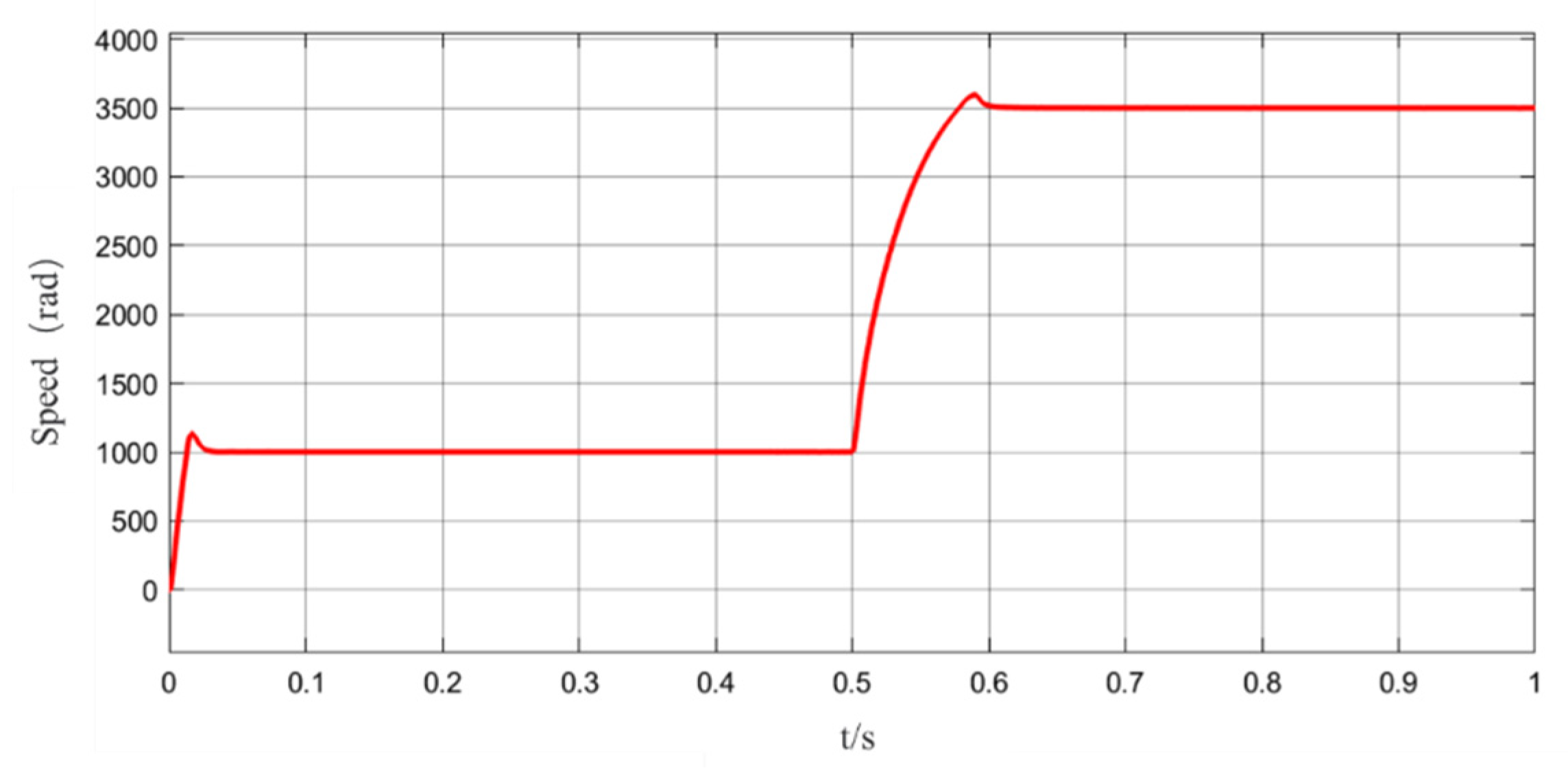
In order to verify the performance of the proposed super-twisting sliding mode model reference adaptation (STSM−MRAS) algorithm, simulation experiments are compared with the traditional MRAS algorithm. The initial running speed of the motor is set as 1000 r/min by simulation. The initial load torque of the motor belt is 10 N∙m. When the simulation model is carried out to 0.5 s, the speed of the motor is suddenly changed to 3500 r/min. Figure 10 shows the simulation waveform of motor speed when speed mutation occurs. Figure 11 shows the simulation waveform of motor speed error under speed mutation. It can be seen from Figure 10 that the motor speed response curves of the traditional MRAS algorithm and the STSM−MRAS algorithm are basically the same in the case of speed mutation.

It can be seen from Figure 11 that in the process of motor startup, the error between the actual speed and the estimated speed of the traditional MRAS algorithm is 46 r/min at most. The maximum speed error of STSM−MRAS algorithm is 33 r/min. Then the motor enters the stable running state. The speed error of the traditional MRAS algorithm converges to zero in 0.075 time. The speed error of STSM−MRAS algorithm converges to zero in 0.055 s. In the motor speed from 1000 r/min to 3500 r/min transition process, the maximum speed error of the traditional MRAS algorithm is 40 r/min. The maximum speed error of STSM−MRAS algorithm is 32 r/min. Then the motor enters the stable running state again. The speed error of the traditional MRAS algorithm converges to zero in 0.62 s. The speed error of TSM-MRAS algorithm converges to zero in 0.61 s.

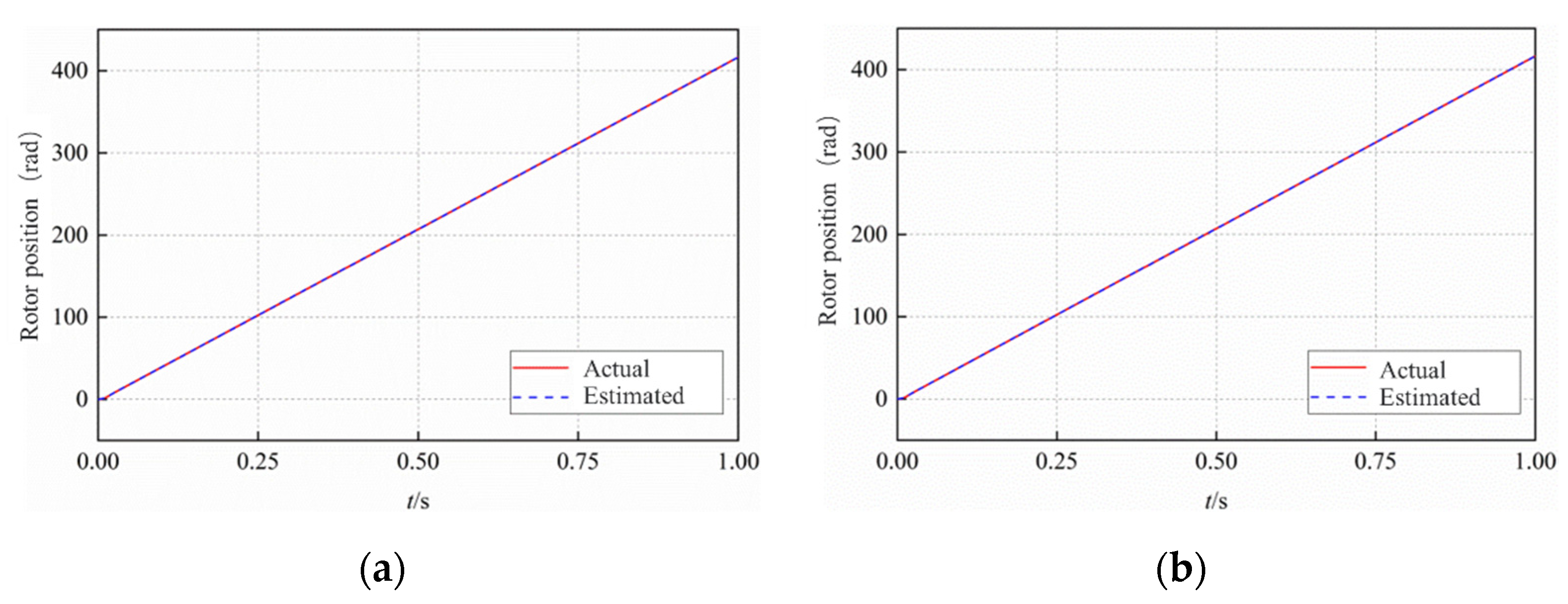
As can be seen from Figure 12, in the case of sudden changes in speed, the rotor position simulation curves of traditional MRAS algorithm and STSM−MRAS algorithm are basically consistent. The estimated rotor position of the motor can always track the actual rotor position.

As can be seen from Figure 13, in the process of motor startup, the mechanical angle error between the actual rotor position and the estimated rotor position of the traditional MRAS algorithm is 0.036 rad. The maximum mechanical angle error of STSM−MRAS algorithm is 0.011 rad. Then the motor enters the stable running state. The rotor position error of the traditional MRAS algorithm converges to zero in 0.08 time. The time for the rotor position error of STSM−MRAS algorithm to converge to zero is 0.06 s. In the motor speed from 1000 r/min to 3500 r/min transition process, the mechanical angle error of the traditional MRAS algorithm is 0.037 rad. The maximum mechanical angle error of the STSM−MRAS algorithm is 0.023 rad. Then the motor enters the stable running state again. The rotor position error of the traditional MRAS algorithm converges to zero in 0.62 s. The time for the rotor position error of STSM−MRAS algorithm to converge to zero is 0.61 s.

The following experiments are designed to further verify the stability of the algorithm. The initial running speed of the motor is set as 1000 r/min by simulation, and the initial load torque of the motor belt is 10 N∙m. When the simulation model is carried out to 0.5 s, the load torque of the motor is changed to 20 N∙m. Figure 14 shows the simulation waveform of motor speed when the motor load torque changes abruptly. Figure 15 shows the simulation waveform of motor speed error when the motor load torque changes abruptly. Figure 16 shows the rotor position simulation waveform when the motor load torque changes abruptly. Figure 17 shows the simulation waveform of rotor position error when the motor load torque changes abruptly.

As can be seen in Figure 14, in the case of torque mutation in constant torque area, the estimated speed of the motor by the two algorithms can always track the actual speed. When the load torque is suddenly changed at 0.5 s, the motor speed of the traditional MRAS algorithm has a drop of about 70 r/min. The motor speed of STSM−MRAS algorithm drops at 65 r/min.

As can be seen in Figure 15, in the process of motor startup, the error between the actual speed and the estimated speed of the traditional MRAS algorithm is 46 r/min. The maximum speed error of STSM−MRAS algorithm is 33 r/min. When the motor enters the stable running state, the speed error of the traditional MRAS algorithm converges to zero in 0.075 s. The speed error of STSM−MRAS algorithm converges to zero in 0.055 s. When the load torque of the motor is changed from 10 N∙m to 20 N∙m in 0.5 s, the maximum speed error of the traditional MRAS algorithm is 18 r/min. The maximum speed error of the STSM−MRAS algorithm is 13 r/min. When the motor enters the stable running state again, the speed error of the traditional MRAS algorithm converges to zero in 0.56 s. The speed error of STSM−MRAS algorithm converges to zero in 0.53 s. This means that the STSM−MRAS algorithm has better robustness than the traditional MRAS algorithm.

As can be seen in Figure 16, in the case of torque mutation in constant torque area, the rotor position simulation curves of the two algorithms are basically the same. The estimated rotor position of the motor can always track the actual rotor position.

As can be seen in Figure 17, in the process of motor startup, the mechanical angle error between the actual rotor position and the estimated rotor position of the traditional MRAS algorithm is 0.036 rad. The maximum mechanical angle error of the STSM−MRAS algorithm is 0.011 rad. When the motor enters the stable running state, the rotor position error of the traditional MRAS algorithm converges to zero in 0.08 s. The time for the rotor position error of STSM−MRAS algorithm to converge to zero is 0.06 s. When the load torque of the motor is changed from 10 N∙m to 20 N∙m in 0.5 s, the maximum mechanical angle error of the traditional MRAS algorithm is 0.0065 rad. The maximum mechanical angle error of STSM−MRAS algorithm is 0.0023 rad. When the motor enters the stable running state again, the rotor position error of the traditional MRAS algorithm converges to zero in 0.56 s. The time for the rotor position error of STSM−MRAS algorithm to converge to zero is 0.53 s.

Compared with the traditional MRAS algorithm, the STSM−MRAS algorithm can reduce the fluctuation of rotor speed and position estimation errors, and make the speed and position estimation errors converge to zero faster under the condition of motor speed mutation and load torque mutation. This shows that the STSM−MRAS algorithm has better steady-state performance.

In the actual running process of PMSM, its parameters will change with changes in the working environment. In particular, the influence of temperature, magnetic field and other factors on inductance parameters is very obvious. The normal operation of PMSM is affected. To verify the robustness of the proposed STSM−MRAS algorithm to the motor parameters after perturbation, the inductance L is set to 120% of the nominal value of the motor, the initial operating speed of the motor is set as 1000 r/min, and the initial load torque of the motor belt is 10 N∙m. When the simulation model is carried out to 0.5 s, the speed of the motor is suddenly changed to 3500 r/min. Figure 18 and Figure 19 show the speed response curves of the two algorithms. Figure 20 and Figure 21 show the torque response curves of the two algorithms.

As can be seen in Figure 18 and Figure 19, under the same working conditions, due to the change of PMSM inductance parameters, the STSM−MRAS algorithm still has a small overshoot after startup and speed change and can quickly reach the given speed value. It reaches the stable state faster than the traditional MRAS algorithm. As can be seen in Figure 20 and Figure 21, when the inductance parameters of PMSM are perturbed, in the case of motor start and speed mutation, then compared with the traditional MRAS algorithm, the STSM−MRAS algorithm has a smaller overshoot and is relatively fast in reaching the stable state. In conclusion, the STSM−MRAS algorithm has better robustness than the traditional MRAS algorithm.

6. Conclusions

In this paper, the position and speed estimation method of the MRAS rotor based on stator current is analyzed theoretically. The reference model equation and adjustable model equation are derived according to the stator current equation. The correctness of the selected linear compensator matrix is strictly proved. Based on Popov’s super stability theory, the speed adaptive law is derived and its asymptotic stability is proved. Based on the voltage closed-loop feedback MTPA weak magnetic control system and the principle of MRAS, a simulation model of MRAS control based on stator current is built. Aiming to solve the problem that the PI adaptive law in the traditional MRAS algorithm is not robust, super-twisting sliding mode control is introduced to replace the PI adaptive law. The MRAS observer based on super-twisting sliding mode is designed and the asymptotic stability of the system is proved according to Lyapunov function. Under certain working conditions, the STSM−MRAS algorithm and the traditional MRAS algorithm are simulated and compared. The results show that the STSM−MRAS algorithm can improve the steady-state performance and robustness of sensorless control system. The disadvantage of the STSM−MRAS algorithm is that it is complicated in principle and is difficult to apply in engineering practice. In the future, we hope to improve this algorithm and simplify the principle, so that the application level of the algorithm can be more extensive. Unfortunately, the paper only carried out simulation verification on the simulation platform without experimental verification. The next step is to carry out experimental verification through the platform test.

References

- Hezzi, A.; Bensalem, Y.; Ben Elghali, S.; Naceur Abdelkrim, M. Sliding Mode Observer based sensorless control of five phase PMSM in electric vehicle. In Proceedings of the 2019 19th International Conference on Sciences and Techniques of Automatic Control and Computer Engineering (STA), Sousse, Tunisia, 24–26 March 2019. [Google Scholar]
- Zhao, K.; Yin, T.; Zhang, C.; He, J.; Li, X.; Chen, Y.; Zhou, R.; Leng, A. Robust Model-Free Nonsingular Terminal Sliding Mode Control for PMSM Demagnetization Fault. IEEE Access 2019, 7, 15737–15748. [Google Scholar] [CrossRef]
- Gu, D.; Yao, Y.; Zhang, D.M.; Cui, Y.B.; Zeng, F.Q. Matlab/Simulink Based Modeling and Simulation of Fuzzy PI Control for PMSM. Procedia Comput. Sci. 2020, 166, 195–199. [Google Scholar] [CrossRef]
- Sarsembayev, B.; Suleimenov, K.; Do, T.D. High Order Disturbance Observer Based PI-PI Control System With Tracking Anti-Windup Technique for Improvement of Transient Performance of PMSM. IEEE Access 2021, 9, 66323–66334. [Google Scholar] [CrossRef]
- Guo, Q.; Pan, T.; Liu, J.; Chen, S. Explicit model predictive control of permanent magnet synchronous motors based on multi-point linearization. Trans. Inst. Meas. Control 2021, 43, 2872–2881. [Google Scholar] [CrossRef]
- Wang, Y.; Yu, H.; Che, Z.; Wang, Y.; Liu, Y. The Direct Speed Control of Pmsm Based on Terminal Sliding Mode and Finite Time Observer. Processes 2019, 7, 624. [Google Scholar] [CrossRef]
- Li, L.; Xiao, J.; Zhao, Y.; Liu, K.; Peng, X.; Luan, H.; Li, K. Robust position anti-interference control for PMSM servo system with uncertain disturbance. CES Trans. Electr. Mach. Syst. 2020, 4, 151–160. [Google Scholar] [CrossRef]
- Nicola, M.; Nicola, C.-I. Sensorless Fractional Order Control of PMSM Based on Synergetic and Sliding Mode Controllers. Electronics 2020, 9, 1494. [Google Scholar] [CrossRef]
- Gao, X.; Sun, B.; Hu, X.; Zhu, K. Echo State Network for Extended State Observer and Sliding Mode Control of Vehicle Drive Motor with Unknown Hysteresis Nonlinearity. Math. Probl. Eng. 2020, 2020, 2534038. [Google Scholar] [CrossRef]
- Liu, K.; Hou, C.; Hua, W. A Novel Inertia Identification Method and Its Application in PI Controllers of PMSM Drives. IEEE Access 2019, 7, 13445–13454. [Google Scholar] [CrossRef]
- Zhao, Y.; Liu, X.; Zhang, Q. Predictive Speed-Control Algorithm Based on a Novel Extended-State Observer for PMSM Drives. Appl. Sci. 2019, 9, 2575. [Google Scholar] [CrossRef] [Green Version]
- Xu, W.; Jiang, Y.; Mu, C.; Blaabjerg, F. Improved Nonlinear Flux Observer-Based Second-Order SOIFO for PMSM Sensorless Control. IEEE Trans. Power Electron. 2018, 34, 565–579. [Google Scholar] [CrossRef]
- Gao, P.; Zhang, G.; Lv, X. Model-Free Control Using Improved Smoothing Extended State Observer and Super-Twisting Nonlinear Sliding Mode Control for PMSM Drives. Energies 2021, 14, 922. [Google Scholar] [CrossRef]
- Gao, P.; Zhang, G.; Lv, X. Model-Free Hybrid Control with Intelligent Proportional Integral and Super-Twisting Sliding Mode Control of PMSM Drives. Electronics 2020, 9, 1427. [Google Scholar] [CrossRef]
- Quynh, N.V. The Fuzzy PI Controller for PMSM’s Speed to Track the Standard Model. Math. Probl. Eng. 2020, 2020, 1698213. [Google Scholar] [CrossRef]
- Fnaiech, M.; Guzinski, J.; Trabelsi, M.; Kouzou, A.; Benbouzid, M.; Luksza, K. MRAS-Based Switching Linear Feedback Strategy for Sensorless Speed Control of Induction Motor Drives. Energies 2021, 14, 3083. [Google Scholar] [CrossRef]
- Dybkowski, M.; Orlowska-Kowalska, T.; Tarchała, G. Sensorless Traction Drive System with Sliding Mode and MRASCC Estimators using Direct Torque Control. Automatika 2013, 54, 329–336. [Google Scholar] [CrossRef]
- Zbede, Y.B.; Gadoue, S.M.; Atkinson, D.J. Model Predictive MRAS Estimator for Sensorless Induction Motor Drives. IEEE Trans. Ind. Electron. 2016, 63, 3511–3521. [Google Scholar] [CrossRef]
- Asfu, W.T. Stator Current-Based Model Reference Adaptive Control for Sensorless Speed Control of the Induction Motor. J. Control Sci. Eng. 2020, 2020, 8954704. [Google Scholar] [CrossRef]
- Zhou, K.; Ai, M.; Sun, Y.; Wu, X.; Li, R. PMSM Vector Control Strategy Based on Active Disturbance Rejection Controller. Energies 2019, 12, 3827. [Google Scholar] [CrossRef]
- Tian, Y.; Chai, Y.; Feng, L. Simultaneous Load Disturbance Estimation and Speed Control for Permanent Magnet Synchronous Motors in Full Speed Range. Appl. Sci. 2020, 10, 9006. [Google Scholar] [CrossRef]
- Qu, L.; Qiao, W.; Qu, L. An Enhanced Linear Active Disturbance Rejection Rotor Position Sensorless Control for Permanent Magnet Synchronous Motors. IEEE Trans. Power Electron. 2019, 35, 6175–6184. [Google Scholar] [CrossRef]
- Choi, K.; Kim, Y.; Kima, K.-S.; Kimb, S.-K. Using the Stator Current Ripple Model for Real-Time Estimation of Full Parameters of a Permanent Magnet Synchronous Motor. IEEE Access 2019, 7, 33369–33379. [Google Scholar] [CrossRef]
- Rui, Z.; Xinhong, X.; Lianbo, C.; Shifeng, G.; Yanhui, Z.; Daoqi, L.; Wei, F. Design of PI Controller for PMSM using Chaos Particle Swarm Optimization Algorithm. IOP Conf. Ser. Mater. Sci. Eng. 2020, 717, 012021. [Google Scholar] [CrossRef]
- Shao, M.; Deng, Y.; Li, H.; Liu, J.; Fei, Q. Sliding Mode Observer-Based Parameter Identification and Disturbance Compensation for Optimizing the Mode Predictive Control of PMSM. Energies 2019, 12, 1857. [Google Scholar] [CrossRef]
- Wang, A.; Wei, S. Sliding Mode Control for Permanent Magnet Synchronous Motor Drive Based on an Improved Exponential Reaching Law. IEEE Access 2019, 7, 146866–146875. [Google Scholar] [CrossRef]
- Yiguang, C.; Chenghan, L.; Zhenmao, B.; Xiaobin, Z. Modified Super-Twisting Algorithm with an Anti-Windup Coefficient Adopted in PMSM Speed Loop Control. Energy Procedia 2019, 158, 2637–2642. [Google Scholar] [CrossRef]
- Toloue, S.F.; Kamali, S.H.; Moallem, M. Multivariable sliding-mode extremum seeking PI tuning for current control of a PMSM. IET Electr. Power Appl. 2020, 14, 348–356. [Google Scholar] [CrossRef]
- Zhang, M.; Xiao, F.; Shao, R.; Deng, Z. Robust Fault Detection for Permanent-Magnet Synchronous Motor via Adaptive Sliding-Mode Observer. Math. Probl. Eng. 2020, 2020, 9360939. [Google Scholar] [CrossRef]
- Gao, P.; Lv, X.; Ouyang, H.; Mei, L.; Zhang, G. A Novel Model-Free Intelligent Proportional-Integral Supertwisting Nonlinear Fractional-Order Sliding Mode Control of PMSM Speed Regulation System. Complexity 2020, 2020, 8405453. [Google Scholar] [CrossRef]
- Zhao, K.; Yin, T.; Zhang, C.; Li, X.; Chen, Y.; Li, T.; He, J. Sliding mode-based velocity and torque controllers for permanent magnet synchronous motor drives system. J. Eng. 2019, 2019, 8604–8608. [Google Scholar] [CrossRef]
- Guoqing, Z.; Xinhong, X.; Yousheng, Z.; Yanhui, Z.; Lianbo, C.; Xinyu, W.; Wei, F. Research on Position Sensorless Control of PMSM Based on Improved SMO. IOP Conf. Ser. Mater. Sci. Eng. 2019, 533, 012019. [Google Scholar] [CrossRef]
- Urbanski, K.; Janiszewski, D. Sensorless Control of the Permanent Magnet Synchronous Motor. Sensors 2019, 19, 3546. [Google Scholar] [CrossRef] [PubMed]
- Jiang, J.; Zhou, X. A robust and fast sliding mode controller for position tracking control of permanent magnetic synchronous motor. E3S Web Conf. 2019, 95, 03002. [Google Scholar] [CrossRef]
- Zaihidee, F.M.; Mekhilef, S.; Mubin, M. Robust Speed Control of PMSM Using Sliding Mode Control (SMC)—A Review. Energies 2019, 12, 1669. [Google Scholar] [CrossRef] [Green Version]
Figure 1.
Equivalent winding diagram of PMSM in d-q coordinate system. (a) d axis equivalent circuit. (b) q axis equivalent circuit.
Figure 2.
Basic structure of model reference adaptive control system.
Figure 3.
Structure diagram of equivalent nonlinear feedback system.
Figure 4.
Block diagram of MRAS rotor position and speed estimation system.
Figure 5.
Block diagram of MRAS control system based on stator current.
Figure 6.
Simulation model of MRAS control system based on stator current.
Figure 7.
Block diagram of rotor position and speed estimation system.
Figure 8.
Block diagram of STSM−MRAS control system.
Figure 9.
Simulation model of STSM−MRAS control system.
Figure 10.
Simulation waveform of motor speed when speed mutation occurs. (a) Traditional MRAS algorithm. (b) STSM−MRAS algorithm.
Figure 11.
Simulation waveform of motor speed error with speed mutation. (a) Traditional MRAS algorithm. (b) STSM−MRAS algorithm.
Figure 12.
Simulation waveform of rotor position under speed mutation. (a) Traditional MRAS algorithm. (b) STSM−MRAS algorithm.
Figure 13.
Simulation waveform of rotor position error with speed mutation. (a) Traditional MRAS algorithm. (b) STSM−MRAS algorithm.
Figure 14.
Simulation waveform of motor speed under sudden change of load torque. (a) Traditional MRAS algorithm. (b) STSM−MRAS algorithm.
Figure 15.
Simulation waveform of motor speed error under load torque mutation. (a) Traditional MRAS algorithm. (b) STSM−MRAS algorithm.
Figure 16.
Simulation waveform of rotor position under sudden change of load torque. (a) Traditional MRAS algorithm. (b) STSM−MRAS algorithm.
Figure 17.
Simulation waveform of rotor position error under sudden change of load torque. (a) Traditional MRAS algorithm. (b) STSM−MRAS algorithm.
Figure 18.
Speed response curve of MRAS algorithm.
Figure 19.
Speed response curve of STSM−MRAS algorithm.
Figure 20.
Torque response curve of MRAS algorithm.
Figure 21.
Torque response curve of STSM−MRAS algorithm.