Article

Simultaneous Minimization of Energy Losses and Greenhouse Gas Emissions in AC Distribution Networks Using BESS

by
Federico Molina-Martin
1,
Oscar Danilo Montoya
2,3,
Luis Fernando Grisales-Noreña
4,
Jesus C. Hernández
5,* and
Carlos A. Ramírez-Vanegas
6
1
Departamento de Ingeniería Eléctrica, Campus Lagunillas s/n, University of Jaén, Edificio A3, 23071 Jaén, Spain
2
Facultad de Ingeniería, Universidad Distrital Francisco José de Caldas, Bogotá 11021, Colombia
3
Laboratorio Inteligente de Energía, Universidad Tecnológica de Bolívar, Cartagena 131001, Colombia
4
Grupo GIIEN, Facultad de Ingeniería, Institución Universitaria Pascual Bravo, Campus Robledo, Medellín 050036, Colombia
5
Department of Electrical Engineering, Campus Lagunillas s/n, University of Jaén, Edificio A3, 23071 Jaén, Spain
6
Facultad de Ciencias Básicas, Universidad Tecnológica de Pereira, Pereira 660003, Colombia
*
Author to whom correspondence should be addressed.
Electronics 2021, 10(9), 1002; https://doi.org/10.3390/electronics10091002
Submission received: 12 March 2021 / Revised: 17 April 2021 / Accepted: 20 April 2021 / Published: 22 April 2021

Abstract

:
The problem of the optimal operation of battery energy storage systems (BESSs) in AC grids is addressed in this paper from the point of view of multi-objective optimization. A nonlinear programming (NLP) model is presented to minimize the total emissions of contaminant gasses to the atmosphere and costs of daily energy losses simultaneously, considering the AC grid complete model. The BESSs are modeled with their linear relation between the state-of-charge and the active power injection/absorption. The Pareto front for the multi-objective optimization NLP model is reached through the general algebraic modeling system, i.e., GAMS, implementing the pondered optimization approach using weighting factors for each objective function. Numerical results in the IEEE 33-bus and IEEE 69-node test feeders demonstrate the multi-objective nature of this optimization problem and the multiple possibilities that allow the grid operators to carry out an efficient operation of their distribution networks when BESS and renewable energy resources are introduced.

1. Introduction

The problem of the optimal operation of battery energy storage systems (BESSs) in electrical distribution has attracted much interest in the last two decades due to the advances in energy storage and power electronic converter technologies [1,2,3]. The main advantages of including these batteries are as follows: (i) possible greenhouse emissions minimization in power systems fed by fossil generation [4,5]; (ii) improvement of the voltage profiles and the reduction of the grid power losses [6]; (iii) possible reduction of power oscillations caused by uncertainties in the renewable energy resources [7,8,9]; (iv) dynamic active and reactive power compensation using power electronic converters in electric vehicles [10]; and (v) real-time demand management [11]. The main question that must be solved when batteries are included in AC grids is as follows: How must these batteries operate to improve the electrical grid performance? Note that the solution of this question involves the proposition and solution of an optimal multi-period power flow model [12], which is known in the literature as the economic dispatch model when the objective function is concerned with operative cost minimization [2].
Nowadays, BESSs are real options for improving the electrical performance of distribution networks in medium- and low-voltage levels [1,13], since these devices can facilitate peak energy consumption fulfillment, enhance the profits from the integration of renewables and distributed energy sources, help power quality management, and generally reduce distribution network expansion costs [14]. The authors of [15] presented an experimental case with regards of the designing a BESS for urban industrial application in order to improve local power quality. They considered two cases of study, i.e., reactive power compensation and rapid variations of the electricity variations caused by a metro train load and a production of a solar power plant, and they mentioned that these studies were technically successful. In addition, an evaluation of the BESS assessment in a real distribution system in Riyadh, Saudi Arabia, was studied by Almehizia et al. [16]. Numerical results quantify the economic return that BESSs can offer for the electrical distribution grids, thus showing that improving the decision-making of the electric utility can deal with increasing load demand and power quality issues.
To analyze BESS in electrical networks with AC or DC operational technologies, one of the most accepted and currently used models corresponds to the linear representation between the state-of-charge and the power injection/absorption [17,18]. However, even if the battery model can be represented using linear equations, nonlinearities appear due to the nonlinear non-convex behaviors in AC power grids, which are caused by the power balance equations [1,19]. To address the nonlinear economic dispatch problem involving BESS and renewable generation in AC grids, various optimization models with different grades of approximation can be used. The first model corresponds to the adaption of the classical economic dispatch model for thermal power systems that uses a unique nodal representation of the system [18]; the second model is the DC approximation of the power flow equations that works with the angular difference between two adjacent nodes by assuming that the voltage is equal to 1.0 pu [20]; and the third model corresponds to the complete AC power flow model that involves active and reactive power balance as well as voltage magnitudes and angles [21]. Note that the two first models are linear programming models, i.e., these are convex models, while the third model is nonlinear and non-convex due to the products among trigonometric functions and voltages in the power balance equations [22].
In the literature, these models are employed to operate BESS and renewable sources in power systems from the point of view of the economic dispatch approach. Some of these works are presented as follows. The authors of [18] presented a unique nodal model for optimal dispatching batteries in AC microgrids. The resulting linear programming model is solved using the CPLEX solver, and the numerical results show the effect of the load and renewable generation behavior in the battery demeanor regarding state-of-charge and power injection/absorption. Berglund et al. [23] presented a linear-integer programming model to minimize the total cost of the facility, including the peak power demand and the energy costs, with the aim of extending battery lifespan. The proposed model uses a unique nodal representation and its solution is reached by using the GAMS optimization package. The authors of [2,20,24,25] presented linear programming and integer-linear programming models for installing and operating BESS in power systems using the DC equivalent of the AC power flow problem. The main aims of these works are the minimization of the investment costs in power systems regarding new transmission lines and the reduction of the greenhouse gas emissions produced by conventional thermal power sources. Most of these models have been solved using the GAMS software. The authors of [17,26,27] evaluated the complete AC multi-period optimal power flow model for the operation of BESS, considering a daily demand curve and renewable generation penetration including apparent power capabilities of the electronic convertors that are interconnected to the BESS. The authors of [21] proposed a nonlinear programming model with continuous an integer variables to install and operate batteries in distribution grids to reduce the total costs of the power losses during daily operation. The batteries are modeled with a binary behavior where the power injection is fixed regarding their maximums and minimums. The solution of this model is reached by implementing a Chu–Beasley genetic algorithm. The authors of [1] proposed an optimization approach to locate and operate BESS and distributed generators in medium- and low-voltage distribution networks, using a hybrid optimization approach that combines the simulating annealing method in the planning stage and a conic decomposition in the operation stage. Three test feeders composed of 11, 135, and 230 nodes are used to validate the proposed optimization methodology, considering the minimization of the investment, operation, and maintenance costs during the planning period. Numerical results demonstrate the effectiveness and robustness of the optimization approach regarding the planning period; however, the authors did not consider terms related to the environmental impact associated with greenhouse gas emissions. In addition, due to the usage of heuristics in the planning stage, the possibility of finding the global optimal is not ensured.
After the revision of the state-of-the-art associated with the optimal integration of BESSs systems in AC distribution grids, the main contributions of this study can be summarized as follows:
The multi-objective formulation of the problem regarding the optimal operation of BESS in AC radial distribution networks using the branch optimal power flow representation, considering the simultaneous minimization of the CO 2 gas emissions and the costs of the daily energy losses, is presented.
The Pareto front is constructed using the multi-objective optimization approach via pondering factors by exploiting the potentialities of the GAMS software for nonlinear optimization.
The different effects that voltage control in the substation and the active and reactive power injection in the BESSs have in the formation of the Pareto front were evaluated.
It is worth mentioning that the scope of this research is focused on the evaluation of different operative scenarios for multi-objective operation of BESSs in radial distribution networks, considering the linear representation of the state-of-charge in batteries and the amount of active power injected (or absorbed) to (or from) the grid, combined with the branch optimal power flow formulation, which has clearly not been proposed in the existing literature. However, it is important to note that even the optimal integration/operation of BESSs in electrical distribution grids can produce important technical and economical profits to the distribution system operators. Such an important fact regarding batteries (i.e., temperature-dependence and time-degradation) must be considered when batteries are installed in distribution grids, since the total expected benefit during its lifespan can be reduced significantly in comparison with ideal operative scenarios. This is an important area of research that the authors of [28] explored for direct current networks, and it can be extrapolated to AC grids in future works using our optimization model that serves as a starting point for future research.
The remainder of this document is organized as follows. Section 2 presents the complete multi-objective formulation of the problem of the optimal operation of BESSs in AC radial distribution networks by using the branch power flow formulation. Section 3 presents the solution methodology to solve the proposed multi-objective optimization problem by using the GAMS software that employs the pondering objective functions strategy. Section 4 shows the main characteristics of the 33-bus test feeder regarding its topology, demand behavior, renewable energy penetration, and BESSs’ locations, among others. Section 5 presents the computational implementation of the proposed multi-objective optimization model to operate BESSs in radial AC grids as well as the main results with their corresponding analysis and discussion. Section 6 presents the main concluding remarks derived from this research as well as possible future directions.

2. Multi-Objective Optimization Problem

The problem of the optimal operation of battery energy storage systems in AC grids is a nonlinear programming (NLP) problem. Here, we adopt the formulation of the power flow problem for strictly radial distribution networks that was proposed by Farivar and Low [19], by extending it to the multi-period domain and including the linear model of the batteries [29]. The complete formulation of the NLP problem is presented below.

2.1. Objective Functions

To operate a BESS in AC distribution systems, we consider two objective functions: the minimization of the CO 2 greenhouse gas emissions and the daily cost of the energy losses in branches. These objective functions are defined as follows:
min z 1 = C O 2 emissions t T i N p 0 i , t ,
min z 2 = C a v e energy t T i j L R i j I i j , t 2 ,
where z 1 is the value of the objective function associated with the total emissions of CO 2 to the atmosphere by diesel generators, z 2 is the cost of the total energy losses in all the branches of the energy, C O 2 emissions is the rate of CO 2 emissions, p 0 i , t is the active power generation that leaves the substation, i.e., root node, to node i, C a v e energy is the average cost of the energy, R i j is the resistance associated with the distribution line that connects nodes i and j, and I i j , t represents the magnitude of the current that flows through the line i j at the period of time t. Observe that N and T are the sets that contain all the nodes of the grid and the periods of time of the study horizon.

2.2. Set of Constraints

The set of constraints associated with the operation of the BESS in electrical AC grids is composed of two main subsets, which are associated with the conventional power flow equations and the battery operation characteristics. Equations (3)–(6) present the conventional power flow equations formulated via branch model as presented in [30]:
p i j , t R i j I i j , t 2 k : j , k L p j k , t = P j , t p j , t d g p j , t b , j N , t T
q i j X i j I i j , t 2 k : j , k L q j k , t = Q j , t q j , t d g q j , t b , j N , t T
V j , t 2 = V i , t 2 2 R i j p i j , t + X i j q i j , t + R i j 2 + X i j 2 I i j , t 2 , ( i , j ) L , t T ,
I i j , t 2 = p i j , t 2 + q i j , t 2 V i , t 2 , ( i , j ) L , t T ,
where p i j , t and q i j , t are the active and reactive power flows leaving node i to travel towards node j in a period of time t. p j k , t and q j k , t have the same definition applied to nodes j and k, respectively. Further, P j , t and Q j , t are the active and reactive power consumption measures at node j in a period of time t modeled as constant power loads. p j , t d g and q j , t d g are the active and reactive power generations in the distributed sources in the node j at the period of time t. Moreover, p j , t b and q j , t b correspond to the active and reactive power injections/absorptions in the battery b connected at node j in the period of time t and V i , t and V j , t are the voltage magnitudes in nodes i and j at the period of time t, respectively.
Remark 1.
Observe that the set of constraints in (3)–(6) is nonlinear and non-convex due to the presence of square variables associated with voltages, currents, and powers. However, the main complication of this model corresponds to Expression (6), since it defines the hyperbolic relation between voltages and powers [19].
The subset of constraints associated with batteries, element capacities, and voltage regulation bounds is described as follows:
s o c j , t b = s o c j , t 1 b φ j b p j , t b Δ T , t T , j N ,
p j , t b 2 + q j , t b 2 s j b , max 2 , t T , j N ,
p j , t b , min p j , t b p j , t b , max , t T , j N ,
s o c j b , min s o c j , t b s o c j b , max , t T , j N ,
p j , t g d , min p j , t g d p j , t g d , max , t T , j N ,
p j , t g d 2 + q j , t g d 2 s j g d , max 2 , t T , j N ,
V j , t min V j , t V j , t max , t T , j N ,
where s o c j , t b is the state-of-charge of the BESS connected at node j in the period of time t, and φ j b is the battery charging/discharging coefficient. Besides, s o c j b , min and s o c j b , min are the lower and upper limits of the state-of-charge variable (these are lower than one and greater than zero to increment battery lifespan; for Ion-Lithium batteries, these are recommended to be 10 % to 90 % [6]). Note that p j , t b , min and p j , t b , max are the active power limits of the batteries. As such, s j b , max is the upper limit regarding power transference of the BESS installed at node j, p j , t g d , min and p j , t g d , max are the lower and upper power limits of the distributed generators (DGs) connected at the node j in the time period t, s j g d , max is the maximum apparent power capability of the DG connected at node j, and V j , t min and V j , t max represent the minimum and maximum voltage regulation bounds admissible in all nodes of the network.

2.3. Interpretation of the Mathematical Model

The multi-objective optimization model defined in (1)–(13) has the following interpretation: Equations (1) and (2) represent the objective functions associated with the minimization of the CO 2 greenhouse gas emissions, and the cost of the daily energy losses. Equations (3) and (4) correspond to the power balance equation at each node of the network, except in the voltage-controlled source. Equations (5) and (6) define the voltage drop at each branch and the hyperbolic relation between voltages and powers, respectively. Equation (7) determines the linear relationship between the state-of-charge and the power injection/absorption at each BESS [18]. Inequality constraints (8)–(10) define the apparent power circle of the battery, the maximum and minimum bounds associated with the active power injection/absorption, and state-of charge, respectively. Inequality expressions (11) and (12) define the distributed generation limits regarding apparent and active power generations. Finally, Expression (13) is known as the voltage regulation constraint, which defines the admissible voltage variations in all the nodes of the network.
Remark 2.
The solution of the mathematical model, (1)–(13), requires powerful optimization tools since this is a nonlinear, non-convex optimization problem with multiple variables defined in the continuous domain. Here, to solve this NLP problem, we adopt the implementation presented in [31], where the GAMS optimization package has been employed to solve a single-objective optimization problem regarding BESS selection and location. This implies that, in this paper, we extend the application of this software for multi-objective optimization problems as described in [2] for power system applications.

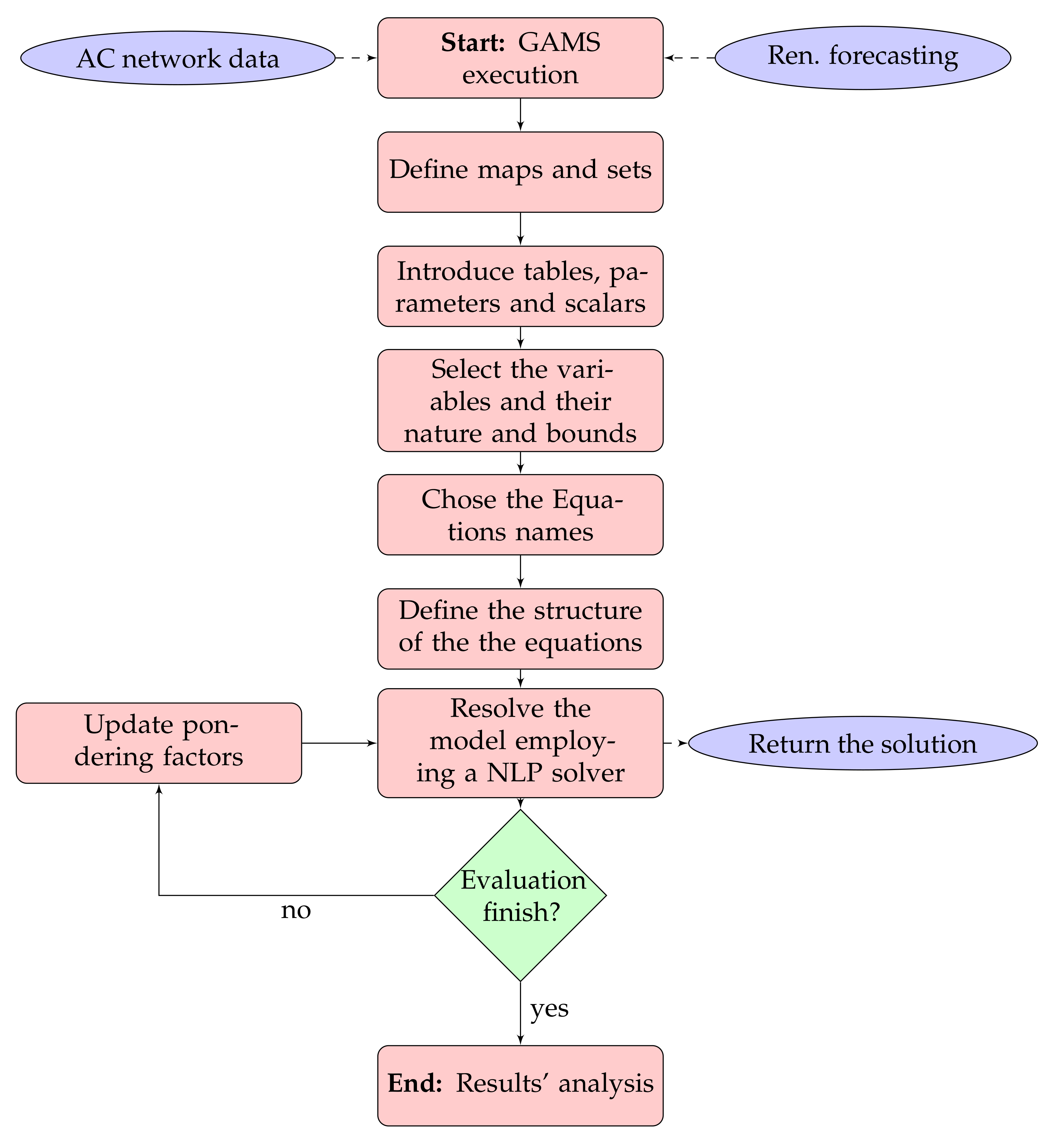
3. Solution Methodology

To resolve the nonlinear programming model defined in (1)–(13), the GAMS software was selected in this research. This software can solve different single-objective optimization problems starting from linear programming, nonlinear programming, and, in general, mixed-integer nonlinear programming problems [2]. However, we adapted this software via loops to solve the proposed NLP problem for multi-objective operation of batteries using the well-known pondering factors approach [32,33]. Table 1 summarizes some studies that worked with the GAMS software to solve different optimization problems to demonstrate its potential applications.
In Table 1, we can observe that, in the literature, there are multiple optimization problems solved with the GAMS software. This demonstrates that this is an excellent tool to address complex programming models such as the case of the multi-objective operation of BESSs in AC grids study in this research.
In general, the implementation of an optimization model in the software GAMS has the following main steps [50]:
  • Define the sets associated with the groups of variables of the problem, i.e., set of periods of time T , set of nodes N , and set of branches L .
  • Define the scalars, parameters (vectors), and tables (matrices), i.e., active and reactive power demands ( P j , t and Q j , t ), resistances and inductances per distribution line ( R i j and X i j ), and the maximum and minimum bounds of the variables (i.e., p j , t b , min , p j , t b , max , s o c j b , min , s o c j b , max , and so on).
  • Define the variables and their natures, i.e., continuous, binary, or discrete.
  • Redact the equation names associated with each of the expressions in the optimization model, as well as the mathematical formulation of these equations using symbolic structure.
  • Select the direction of the optimization, i.e., minimization, and the nature of the problem for being solved, i.e., NLP.
Remark 3.
The implementation of an optimization model in the software GAMS requires some familiarization with its syntax and general structure, since it works using plain text to formulate the complete mathematical model. For more details about the GAMS usage, see the works by Soroudi [2] and Castillo et al. [50].
A schematic implementation of an optimization model using the GAMS software is depicted using a general flow chart in Figure 1.

4. Information of the Test Feeders

This section presents the parametric information of the test feeders considered for validating the multi-objective operation of BESSs in rural distribution grids fed by diesel sources. The first test feeder corresponds to the IEEE 33-node test feeder and the second is the IEEE 69-node test feeder. All information regarding both distribution grids is presented below.

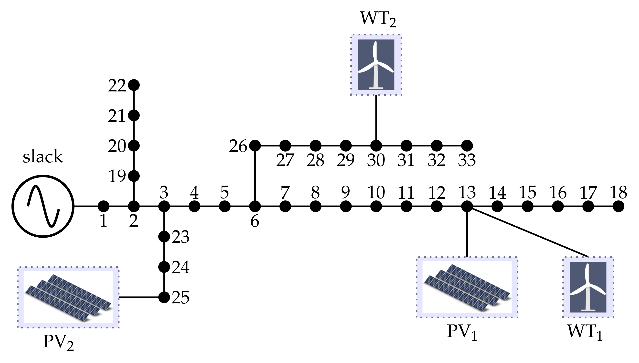
4.1. IEEE 33-Node Test Feeder

The IEEE 33-bus test feeder, which is a radial distribution network composed of 33 buses and 32 distribution lines, is operated at 12.66 kV at the substation bus (i.e., bus 1). The electrical connection between buses in the 33-bus test feeder is presented in Figure 2 and the parametric information of this test feeder is presented in Table 2. It is important to highlight that the information presented in this table corresponds to the load peak consumption in all the nodes of the system, which is surmised of 3715 kW and 2300 kvar. In addition, it is considered here that this medium-voltage distribution network is located in a rural area, where the main substation corresponds to a diesel generator, as reported in [27].
In this electrical network, the existence of four distributed generators is also considered: two of them arise from solar photovoltaic technology and two of them work with wind generation technology. The location of these distributed generators is as follows: (i) the PV 1 source is installed at node 13 with a capacity of generation defined as 450 kW and the PV 2 source is located at node 25 with a capability of 1500 kW; and (ii) the WT 1 source is connected at the same node as the PV 1 source with a nominal capacity of 825 kW and the PV 2 is sited at node 30 with a rate of generation defined as 1200 kW. The information associated with the distributed sources and demand is listed in Table 3.
It is worth mentioning that the information regarding renewable generation presented in Table 3 was obtained by using an artificial neural network (ANN) to predict the daily generation considering a year of historic information that contains data about solar radiation, wind speed, humidity, pressure, and time. The complete information related to the implementation of the ANN can be found in [38], and some aspects regarding the ANN implementation are provided in Appendix A.
Regarding the location and sizing of the BESSs, we consider the information reported in [27] that includes three batteries allocated in this test feeder: (i) a BESS with an energy capacity of 1000 kWh that can be charged/discharged in 4 h (Battery Type A); (ii) a BESS with an energy capacity of 1500 kWh that can be charged/discharged in 4 h (Battery Type B); and (iii) a BESS with an energy capacity of 2000 kWh that can be charged/discharged in 5 h (Battery Type C). Observe that the power injection/absorption of the battery can be calculated by dividing the energy rate by the total charging/discharging time, i.e., for the Battery Type A, this power injection/absorption is 250 kW. In addition, to define the location of these batteries, we consider the solution reported in [31] that defines that Battery Types A–C are located at nodes 14, 31, and 6, respectively.
To evaluate the objective functions associated with the minimization of the greenhouse emissions and the daily energy loss costs, we consider that the diesel generator located at node 1 emits about 612.35 kg/MWh and that the average energy costs are assumed to be US$ 0.1390 , as taken from [26], by converting Colombian pesos (COP$ 479.3389 ) to American dollars.

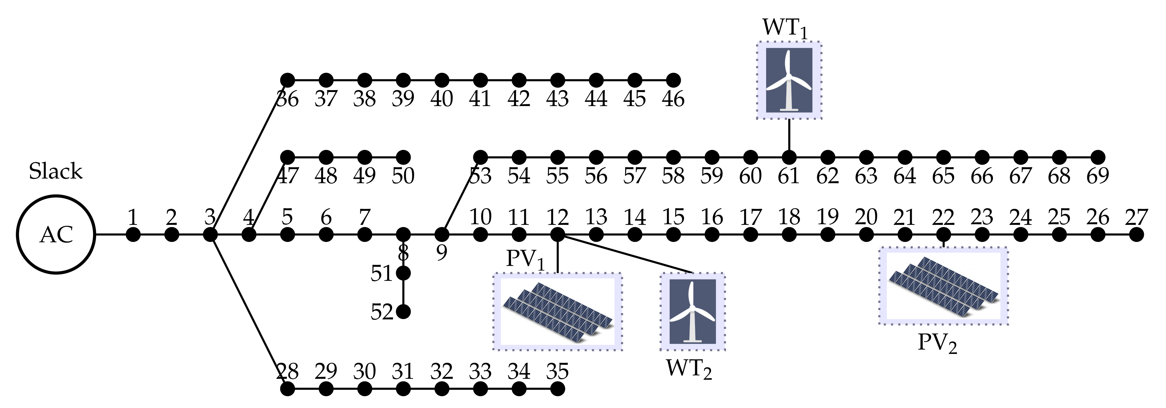
4.2. IEEE 69-Node Test Feeder

The IEEE 69-bus test feeder is a radial distribution network composed of 69 buses and 69 distribution lines, which is operated at 12.66 kV at the substation bus (i.e., bus 1). The electrical connection between buses in the 69-bus test feeder is presented in Figure 3 and the parametric information of this test feeder is presented in Table 4. It is important to highlight that the information presented in this table corresponds to the load peak consumption in all nodes of the system, which surmises 3890.70 kW and 2693.6 kvar. In addition, here, it is considered that this medium-voltage distribution network is located in a rural area, where the main substation corresponds to a diesel generator and as reported in [27].
In this electrical network, the existence of four distributed generators is also considered, two of which work with solar photovoltaic technology and two of which work with wind generation technology. The location of these distributed generators is as follows: (i) the PV 1 source is installed at node 12 with a capacity of generation defined as 1050 kW and the PV 2 source is located at node 22 with a capability of 850 kW; and (ii) the WT 1 is sited at node 61 with a rate of generation defined as 760 kW and the WT 2 source is connected to the same node as the PV 1 source with a nominal capacity of 1000 kW. Note that the information of the distributed sources and demand is listed in Table 3.
As this test feeder is considered an additional BESS regarding the batteries considered for the IEEE-33 node test feeder (i.e., Battery Type D), as reported in [27], this is a BESS with an energy capacity of 3000 kWh that can be charged/discharged in 6 h. The location of the BESS Types A–D is at nodes 40, 64, 16, and 9, respectively.

5. Numerical Simulations

This section shows the computational implementation of the proposed multi-objective optimization approach to operate BESSs in AC distribution systems considering the minimization of the greenhouse gas emissions versus costs of daily energy losses. We implemented this approach on a personal computer AMD Ryzen 7 3700U, 2.3 GHz, 16 GB RAM with 64-bits Windows 10 Home Single Language using the GAMS optimization environment.
The construction of the Pareto fronts presented in this section was made by using the weighting factors methodology that combines both objective functions as follows: z comb m = ϑ z 1 + ( 1 ϑ ) z 2 , where ϑ = m / 20 is the pondering factor. Note that m defines the number of combined objective function evaluations. In the proposed study, the parameter m begins from 0 in steps of 1–20. It is worth mentioning that the value of ϑ determines the number of solutions contained in the Pareto front.
For numerical purposes, different simulation cases in this section are presented and applied to the IEEE 33-bust test feeder and the IEEE 69-bus test feeder. For the first distribution grid, we considered the following cases: (i) effect of the substation voltage control; (ii) effect of the reactive power compensation with battery converters; and (iii) effect of the renewable energy variation in the Pareto front conformation. However, for the IEEE 69-node test feeder, to avoid repeating the analysis made in the IEEE 33-node test feeder, we only evaluated the operation of the batteries with unity and variable power factors, given the generators operate in their nominal condition.

5.1. IEEE-Bus Test Feeder

In this subsection, all the simulation scenarios considered for the IEEE-33 bus test feeder are presented, which include the effect of the substation voltage control, the variable power factor capabilities in batteries, and the possible variation of the renewable energy resources.

5.1.1. Effect of the Substation Voltage Control

To demonstrate the effect that has the assignation of the substation voltage in a predefined value, e.g., V 1 = 1.00 0 , we simulated two cases. The first case considers that the substation is controlling the voltage magnitude at 1.00 pu and the second case leaves this voltage magnitudes free, i.e., it can take values from v min to v max . Figure 4 presents the Pareto fronts for both simulation cases.
The results in Figure 4 show the following. In the first case, the minimum and maximum values regarding the costs of energy losses are US$ 132.0450 and US$ 157.1888 , which correspond to total CO 2 emissions of about 13.8714 and 6.5502 tons/day, respectively. The difference between the extreme solutions are US$ 25.1438 and 7.3212 tons/day, respectively. In the second case, the minimum and maximum values regarding the costs of energy losses are US$ 108.1019 and US$ 129.4134 , which correspond to total CO 2 emissions of about 13.8294 and 6.4853 tons/day, respectively. The difference between the extreme solutions are US$ 20.6115 and 7.3441 tons/day, respectively. Finally, the main effect of maintaining the voltage magnitude of the substation in a fixed value (i.e., Case 1), in contrast to the solution reported by Case 2, is associated with an increment in the daily cost of the energy losses about US$ 26.4417 . However, when CO 2 emissions are analyzed, we observe that the average difference is less than 0.0500 tons/day. These results imply that fixing the voltage substation has a direct effect on the energy losses, and that this effect is negative, as shown in Figure 4.
The complete list of the objective function pairs is reported in Table 5, based on the information in Figure 4 from left to right.
Note that results in Table 5 demonstrate the multi-objective nature of the problem of the optimal operation of BESSs in AC grids, since the improvement of one of the objectives implies the deterioration of the other. In addition, observe that Solutions 6–12 can be considered attractive solutions to be selected by the distribution system operator, since these are in the intermediate area of the Pareto, which implies that both objectives perform well regarding their extremes. For example, Solution 9 in Case 1 produces a reduction of about 43.05 % regarding CO 2 emissions and 7.11 % in relation to the maximum energy daily costs; in Case 2, these reductions are 43.08 % and 7.49 % , respectively.

5.1.2. Effect of the Reactive Power Compensation with Battery Converters

In the previous subsection, we evaluate the effect of the voltage control in the substation bus considering unity power factor in the operation of the batteries and distributed generators. In this simulation case, we consider that the substation has free voltage magnitude and the batteries can support reactive power with their converters by assuming that the DGs will continue working with unity power factor [26]. In Figure 5, the Pareto front for the operational BESS, considering the variable power factor, is presented.
From the results in Figure 5, we can observe the following to be true. First, the extreme solutions of the Pareto front correspond to minimum CO 2 emissions of 6.3136 tons/day with a maximum daily energy costs of about US$ 59.1780 , while the maximum value of the CO 2 emissions is 13.9245 tons/day with minimum daily operative costs of US$ 37.5963 . Second, the difference between the extremes corresponds to a reduction of 54.66 % regarding CO 2 emissions, while the costs of daily energy losses is about 34.47 % . Third, when comparing the Pareto front in Figure 5 with Case 2 in the Pareto front presented in Figure 4, it is possible to observe that the injection of the reactive power in batteries allows the reduction of the daily operation costs by about US$ 70 per day, which represents a daily profit of 54.27 % to the grid operator.
To illustrate the behavior of the state-of-charge in batteries, we plot this variable for all the batteries in both extremes (see Figure 6) of the Pareto front in Figure 5.
The behaviors of the BESSs in Figure 6 show that, depending on the objective function prioritized, the BESSs will work with different charging/discharging profiles along the day. Depending on the minimization interest, they decide to store or provide energy in different periods of time (see comparison of batteries in nodes 6 and 14), especially in the period of time between 14 and 28. In addition, note that, in the case of minimizing the daily energy costs, the BESSs start to provide energy continuously from the period of time 16 to the period of time 46, while, in the case of the CO 2 minimization, these behaviors do not occur. This is attributable to the availability of the renewable resources and the demand behavior, which has two main peaks that require additional power injections from the BESS to minimize the amount of power injection in the conventional source that is directly connected with the amount of CO 2 emissions, as seen in Equation (1).

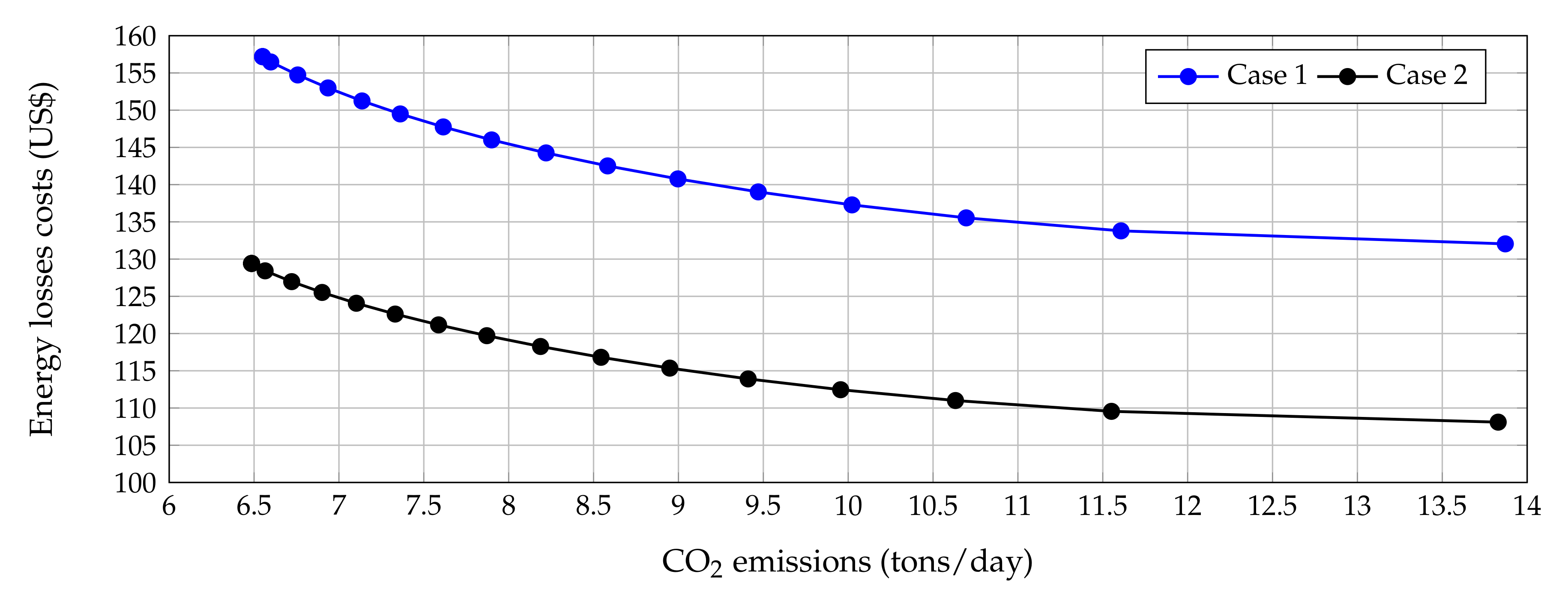
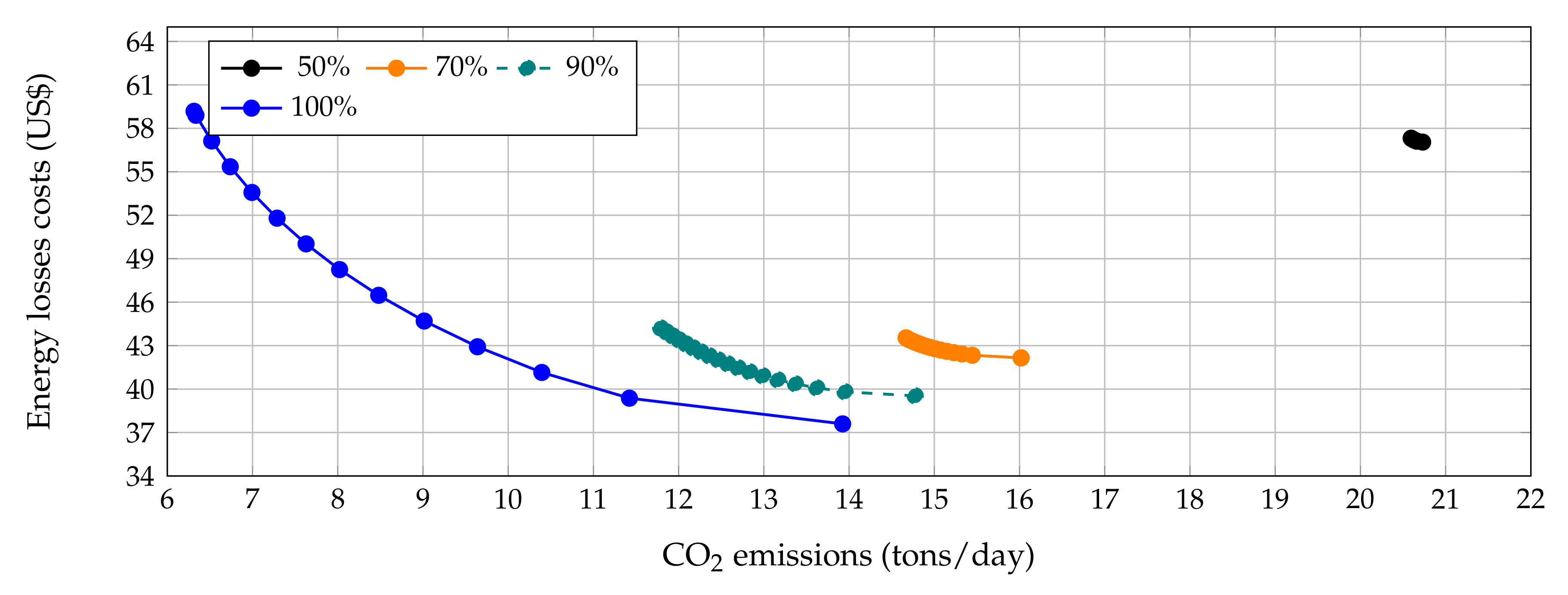
5.1.3. Effect of the Renewable Energy Variation in the Pareto Front Conformation

To present the effect of the renewable energy variation due to the stochastic nature of the primary energy resources, i.e., wind speed and solar radiation, we now present a simulation case where the amount of active power injection from the renewable energy resources varies from 50 % to 100 % for each varying level of renewable energy availability. As such, the Pareto front presented in Figure 7 is obtained, considering unity power factor in the renewable generation, active, and reactive power injections in the BESS, and the free behavior in the slack voltage magnitude.
The following can be noted from the behavior of the Pareto fronts in Figure 6. First, depending on the availability of the renewable energy resources during a day of operation, the Pareto front can be very restricted. For instance, in the case of a renewable energy availability of 50 % , the daily operative costs are between US$ 55 and US$ 58, while CO 2 emissions are between 20 and 21 tons/day. Second, when the amount of active power injection with renewable energy resources increases, the behavior of the Pareto front regarding the CO 2 emissions presents higher differences in their extremes. For example, for an availability of 50 % , the difference between the extreme solutions is about 1.3506 tons/day, and, for a 90 % renewable generation availability, this value is about 2.9869 tons/day. This implies the growing importance of decisions-making regarding the operation of the distribution network on the part of the distribution company when the amount power injection from renewable generation increases. Finally, the biggest effect associated with the availability of the renewable generation to inject active power corresponds to the amount CO 2 emissions, since this variable is directly connected to the total power injection in the slack node, which is then directly connected to the power injections in the distributed generators. This is particularly true while the daily operative costs for all the percentages of penetration between the extremes remain the same in the case of the nominal operation, i.e., 100% of renewable generation availability. These results imply that the BESS can control the grid losses in better form, since it depends on the voltage drops in lines, as compared to the the case of the greenhouse emissions, since these depend directly on the usage of the diesel generator.

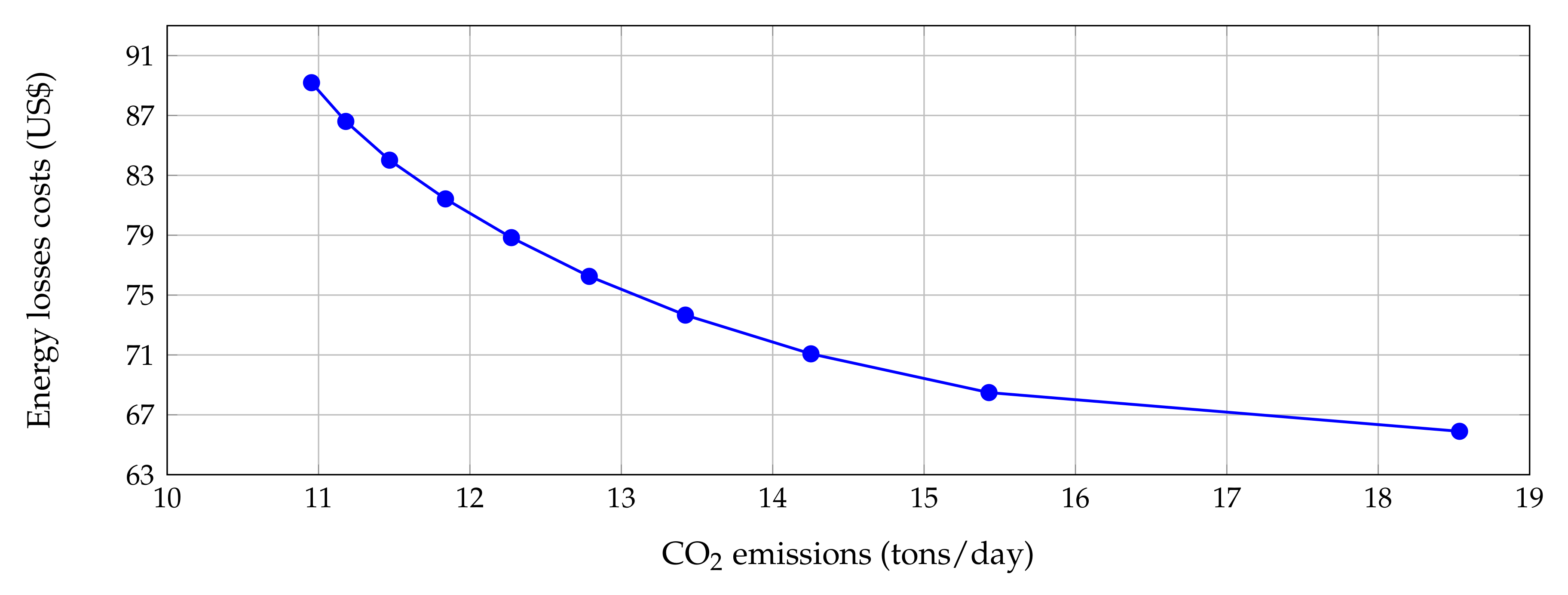
5.2. IEEE 69-Bus Test Feeder

For the IEEE 69-bus test feeder, we consider the possibility of operating the BESSs while considering that the voltage control of the substation is free and can can be moved from 0.90 to 1.10 pu by maintaining its angle at zero for all periods of time. The Pareto front for this test feeder is presented in Figure 8. Note that the extreme solutions in the Pareto front are the following: (i) the minimum daily energy costs is US$ 65.8980 with maximum CO 2 emissions of 18.5373 tons/day; and (ii) the minimum emissions of CO 2 are 10.9535 tons/day, with a maximum daily costs of energy losses of US$ 89.1888.
It is worth mentioning that the difference between the extreme solutions in the Pareto front in Figure 7 is US$ 23.2908 and 7.5838 tons/day. These values imply that, depending on the distribution system operator, the daily indicators can reduce until these values are selected as a function of the operative point. In addition, it is possible to observe that the most promissory solutions that allow minimizing both objective functions are in the region between 12 and 15 tons/day, since these have daily energy loss costs of between US$ 79 and US$ 71.

6. Conclusions

We studied the problem of operation of a BESS in radial AC grids from the multi-objective point of view, considering the simultaneous minimization of CO 2 emissions and the costs of the daily energy losses. The GAMS software combined with the pondering objective functions approach were employed to solve the resulting nonlinear, non-convex, and multi-period optimal power flow problem. Numerical validations demonstrated that the assignation of the voltage magnitude in the substation bus deteriorates the behavior of the optimal Pareto front since both objectives present higher values in comparison with the scenario where voltage magnitude in the substation is left free.
When reactive power injections are available for operating the BESS, considering its power electronic converters, the objective function regarding energy loss costs is drastically reduced. This was made possible since these reactive power injections allowed the improvement of voltage profiles, which is directly connected with the reduction of magnitude of the current in branches. This reduction was about 54.27 % in comparison to the unity factor power case.
The effect of the renewable generation availability was tested for different percentages of active power generation in distributed sources. This demonstrated that the amount of greenhouse gas emissions is directly connected to the power supply by distributed generators, while daily energy losses can be effectively controlled for the BESSs by maintaining these on the extreme values of the nominal operative case, i.e., between US$ 37.5963 and US$ 59.1780 , for all the renewable generation penetration cases evaluated.
In the IEEE 69-bus system, it was observed that the maximum reduction of CO 2 emissions is about 40.91% when the daily cost of energy losses has a maximum value, i.e., US$ 89.1888. In the case of energy losses, the maximum reduction is about 26.11% when the maximum CO 2 emissions occur. These values correspond to the extreme solutions in the Pareto front in Figure 7, which implies that, depending on the distribution system operator’s decision, the maximum improvements possible will be contained in the aforementioned percentages of reduction.
The following research can be developed as part of future research efforts following this paper’s contribution. First, the reformulation of the proposed branch multi-period optimal power flow model for multi-objective operation of the BESS in AC grids with radial structure into a convex conic representation that ensures the global optimum finding from the formal mathematical point of view. Second, the application of proposed multi-objective optimization model to direct current networks with high penetration of renewable energy resources and batteries. Finally, the inclusion of new battery behaviors in the proposed optimization model, such as lifespan and deep discharging characteristics, among others, to approximate the best behavior of these in real operative conditions.

Author Contributions

Conceptualization, F.M.-M., O.D.M., L.F.G.-N., J.C.H., and C.A.R.-V.; Methodology, F.M.-M., O.D.M., L.F.G.-N., J.C.H., and C.A.R.-V.; Investigation, F.M.-M., O.D.M., L.F.G.-N., J.C.H., and C.A.R.-V.; and Review—writing and editing, F.M.-M., O.D.M., L.F.G.-N., J.C.H., and C.A.R.-V. All authors have read and agreed to the published version of the manuscript.

Funding

This research was funded by the Agencia Estatal de Investigación, Spain (AEI) and the Fondo Europeo de Desarrollo Regional (FEDER) aimed at the Challenges of Society (Grant No. ENE 2017-83860-R “Nuevosservicios de red para microredes renovables inteligentes. Contribución a la generación distribuida residencial”).

Data Availability Statement

No new data were created or analyzed in this study. Data sharing is not applicable to this article.

Acknowledgments

This work was supported in part by the Centro de Investigación y Desarrollo Científico de la Universidad Distrital Francisco José de Caldas under Grant 1643-12-2020 associated with the project, “Desarrollo de una metodología de optimización para la gestión óptima de recursos energéticos distribuidos en redes de distribución de energía eléctrica”, and in part by the Dirección de Investigaciones de la Universidad Tecnológica de Bolívar under Grant PS2020002 associated with the project, “Ubicación óptima de bancos de capacitores de paso fijo en redes eléctricas de distribución para reducción de costos y pérdidas de energía: Aplicación de métodos exactos y metaheurísticos”.

Conflicts of Interest

The authors declare no conflict of interest.

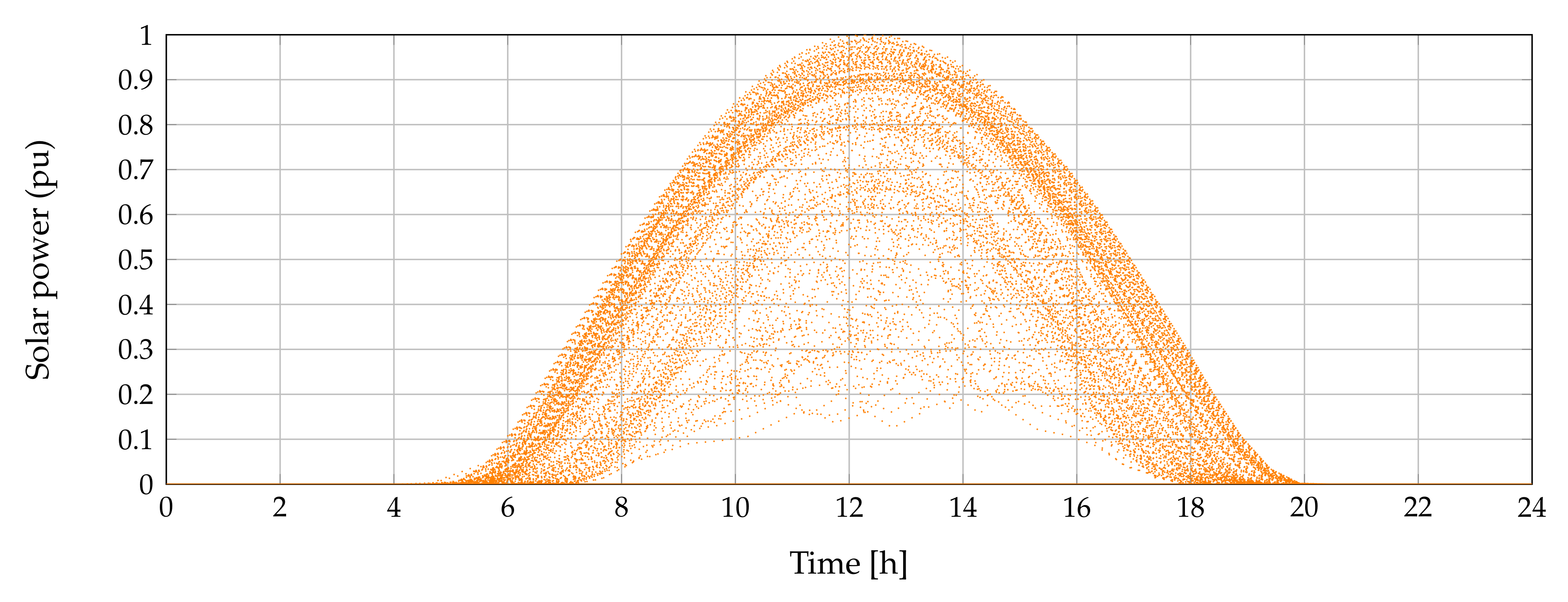
Appendix A. Renewable Generation Forecasting

The renewable generation dependence on the weather conditions associated with solar radiation and temperature for photovoltaic plants make this source non-dispatchable, which clearly affects the grid operation, causing increments in the operative costs, low voltage profile, and high energy losses [26]. For this reason, to operate electric distribution networks in rural and urban areas, it is necessary to have an adequate short-term forecasting approach to estimate the renewable energy output for the next day. In the literature, some approaches are proposed to predict the renewable energy behavior. These include fuzzy logic [52], stochastic optimization methods [53], similar day approach [54], and artificial neural networks [26,55], among others. Here, we employed the methodology proposed in [26] to forecast the renewable energy for the day-ahead operation of the distribution grid.
It is worth mentioning that, for the sake of simplicity, in the ANN implementation, we only present information of the PV prediction. However, the complete details for wind generation forecasting can be seen in [55].

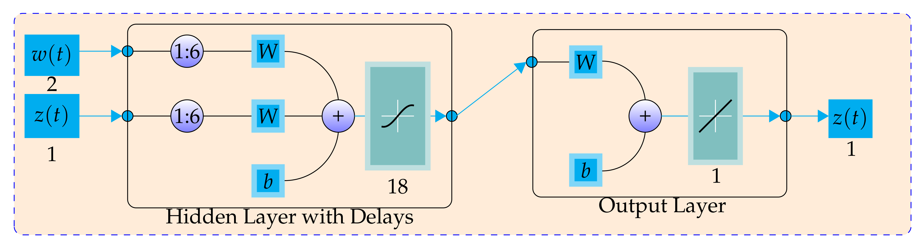
Appendix A.1. Recursive Artificial Neural Network

The application of the ANNs covers a wide range of problems such as pattern classification [56], function approximations [57], clustering [58], and data forecasting [59]. In general, ANNs can be considered as mathematical tools that allow the emulation of the biological neural system. This implies that these can remember and store information and learn to predict future behaviors regarding stochastic variables [26].
The training procedure for an ANN is carried out using an input–output space to reach a nonlinear mapping of the items. This training methodology is adopted when the relations among inputs and outputs are unknown. The general nonlinear learning rule takes the following form:
z ( t ) = f z ( t 1 ) , . . . , z ( t n z ) , w ( t 1 ) , . . . , w ( t n w )
where w defines the input space and z corresponds to the output space, which depends on the previous n z values of the variable under forecast. The input and output spaces for forecasting the PV generation correspond to the temperature and time as well as solar radiation, respectively [26].
The procedure to train the ANN to forecast the solar radiation was carried out using MATLAB software and its ntstool package. Note that, for the solar radiation prediction, two inputs were considered (i.e., temperature and time) along with six delays ( n z = 6 ) and 18 neurons in the hidden layer.

Appendix A.2. Computational Implementation of the Ann

The schematic configuration of the ANN implemented for solar generation forecasting is presented in Figure A1, which was developed using the ntstool package in MATLAB. All the information used to train, adjust, and validate the proposed ANN for solar generation forecasting was taken from [55]. It is worth mentioning that, for training, adjusting, and validation, we employed 70%, 15%, and 15% of the data, respectively. Finally, Figure A2 presents the solar generation information.
Figure A1. ANN scheme for solar radiation prediction [55].
Electronics 10 01002 g0a1
Figure A2. Historical data used for the ANN training process for solar power forecasting.
Electronics 10 01002 g0a2

References

  1. Valencia, A.; Hincapie, R.A.; Gallego, R.A. Optimal location, selection, and operation of battery energy storage systems and renewable distributed generation in medium–low voltage distribution networks. J. Energy Storage 2021, 34, 102158. [Google Scholar] [CrossRef]
  2. Soroudi, A. Power System Optimization Modeling in GAMS; Springer International Publishing: Berlin/Heidelberg, Germany, 2017. [Google Scholar] [CrossRef]
  3. Gonzalez, W.J.G.; Bocanegra, S.Y.; Serra, F.M.; Bueno-López, M.; Magaldi, G.L. Control Methods for Single-phase Voltage Supply with VSCs to Feed Nonlinear Loads in Rural Areas. Trans. Energy Syst. Eng. Appl. 2020, 1, 33–47. [Google Scholar] [CrossRef]
  4. Raugei, M.; Peluso, A.; Leccisi, E.; Fthenakis, V. Life-Cycle Carbon Emissions and Energy Return on Investment for 80% Domestic Renewable Electricity with Battery Storage in California (U.S.A.). Energies 2020, 13, 3934. [Google Scholar] [CrossRef]
  5. Gong, Z.; Chau, S.; Trescases, O. Quantifying the GHG Reduction versus Battery Size in Diesel Buses with Electrified HVAC. In Proceedings of the 2020 IEEE Transportation Electrification Conference & Expo (ITEC), Chicago, IL, USA, 23–26 June 2020. [Google Scholar] [CrossRef]
  6. Grisales-Noreña, L.; Montoya, O.D.; Ramos-Paja, C.A. An energy management system for optimal operation of BSS in DC distributed generation environments based on a parallel PSO algorithm. J. Energy Storage 2020, 29, 101488. [Google Scholar] [CrossRef]
  7. Weniger, J.; Tjaden, T.; Quaschning, V. Sizing of Residential PV Battery Systems. Energy Procedia 2014, 46, 78–87. [Google Scholar] [CrossRef] [Green Version]
  8. Subramaniam, U.; Vavilapalli, S.; Padmanaban, S.; Blaabjerg, F.; Holm-Nielsen, J.B.; Almakhles, D. A Hybrid PV-Battery System for ON-Grid and OFF-Grid Applications—Controller-In-Loop Simulation Validation. Energies 2020, 13, 755. [Google Scholar] [CrossRef] [Green Version]
  9. Zhu, Y.; Liu, C.; Wang, B.; Sun, K. Damping control for a target oscillation mode using battery energy storage. J. Mod. Power Syst. Clean Energy 2018, 6, 833–845. [Google Scholar] [CrossRef] [Green Version]
  10. Kisacikoglu, M.C.; Ozpineci, B.; Tolbert, L.M. Effects of V2G reactive power compensation on the component selection in an EV or PHEV bidirectional charger. In Proceedings of the 2010 IEEE Energy Conversion Congress and Exposition, Atlanta, GA, USA, 12–16 September 2010. [Google Scholar] [CrossRef] [Green Version]
  11. Mazza, A.; Mirtaheri, H.; Chicco, G.; Russo, A.; Fantino, M. Location and Sizing of Battery Energy Storage Units in Low Voltage Distribution Networks. Energies 2019, 13, 52. [Google Scholar] [CrossRef] [Green Version]
  12. Wang, Z.; Zhong, J.; Chen, D.; Lu, Y.; Men, K. A multi-period optimal power flow model including battery energy storage. In Proceedings of the 2013 IEEE Power & Energy Society General Meeting, Vancouver, BC, Canada, 21–25 July 2013. [Google Scholar] [CrossRef]
  13. Aghaei, J.; Bozorgavari, S.A.; Pirouzi, S.; Farahmand, H.; Korpås, M. Flexibility Planning of Distributed Battery Energy Storage Systems in Smart Distribution Networks. Iran. J. Sci. Technol. Trans. Electr. Eng. 2019, 44, 1105–1121. [Google Scholar] [CrossRef]
  14. Das, C.K.; Bass, O.; Kothapalli, G.; Mahmoud, T.S.; Habibi, D. Overview of energy storage systems in distribution networks: Placement, sizing, operation, and power quality. Renew. Sustain. Energy Rev. 2018, 91, 1205–1230. [Google Scholar] [CrossRef]
  15. Heine, P.; Hellman, H.P.; Pihkala, A.; Siilin, K. Battery Energy Storage for Distribution System—Case Helsinki. In Proceedings of the 2019 Electric Power Quality and Supply Reliability Conference (PQ) & 2019 Symposium on Electrical Engineering and Mechatronics (SEEM), Kärdla, Estonia, 12–15 June 2019. [Google Scholar] [CrossRef]
  16. Almehizia, A.A.; Al-Ismail, F.S.; Alohali, N.S.; Al-Shammari, M.M. Assessment of battery storage utilization in distribution feeders. Energy Transit. 2020, 4, 101–112. [Google Scholar] [CrossRef]
  17. Montoya, O.D.; Grajales, A.; Garces, A.; Castro, C.A. Distribution Systems Operation Considering Energy Storage Devices and Distributed Generation. IEEE Lat. Am. Trans. 2017, 15, 890–900. [Google Scholar] [CrossRef]
  18. Luna, A.C.; Diaz, N.L.; Andrade, F.; Graells, M.; Guerrero, J.M.; Vasquez, J.C. Economic power dispatch of distributed generators in a grid-connected microgrid. In Proceedings of the 2015 9th International Conference on Power Electronics and ECCE Asia (ICPE-ECCE Asia), Seoul, Korea, 1–5 June 2015. [Google Scholar] [CrossRef] [Green Version]
  19. Farivar, M.; Low, S.H. Branch Flow Model: Relaxations and Convexification—Part I. IEEE Trans. Power Syst. 2013, 28, 2554–2564. [Google Scholar] [CrossRef]
  20. Mora, C.A.; Montoya, O.D.; Trujillo, E.R. Mixed-Integer Programming Model for Transmission Network Expansion Planning with Battery Energy Storage Systems (BESS). Energies 2020, 13, 4386. [Google Scholar] [CrossRef]
  21. Grisales-Noreña, L.; Montoya, O.D.; Gil-González, W. Integration of energy storage systems in AC distribution networks: Optimal location, selecting, and operation approach based on genetic algorithms. J. Energy Storage 2019, 25, 100891. [Google Scholar] [CrossRef]
  22. Molzahn, D.K. Identifying and Characterizing Non-Convexities in Feasible Spaces of Optimal Power Flow Problems. IEEE Trans. Circuits Syst. II Express Briefs 2018, 65, 672–676. [Google Scholar] [CrossRef]
  23. Berglund, F.; Zaferanlouei, S.; Korpås, M.; Uhlen, K. Optimal Operation of Battery Storage for a Subscribed Capacity-Based Power Tariff Prosumer—A Norwegian Case Study. Energies 2019, 12, 4450. [Google Scholar] [CrossRef] [Green Version]
  24. Denholm, P.; Sioshansi, R. The value of compressed air energy storage with wind in transmission-constrained electric power systems. Energy Policy 2009, 37, 3149–3158. [Google Scholar] [CrossRef]
  25. Mazaheri, H.; Abbaspour, A.; Fotuhi-Firuzabad, M.; Farzin, H.; Moeini-Aghtaie, M. Investigating the impacts of energy storage systems on transmission expansion planning. In Proceedings of the 2017 Iranian Conference on Electrical Engineering (ICEE), Tehran, Iran, 2–4 May 2017. [Google Scholar] [CrossRef]
  26. Montoya, O.D.; Gil-González, W. Dynamic active and reactive power compensation in distribution networks with batteries: A day-ahead economic dispatch approach. Comput. Electr. Eng. 2020, 85, 106710. [Google Scholar] [CrossRef]
  27. Montoya, O.D.; Serra, F.M.; Angelo, C.H.D. On the Efficiency in Electrical Networks with AC and DC Operation Technologies: A Comparative Study at the Distribution Stage. Electronics 2020, 9, 1352. [Google Scholar] [CrossRef]
  28. Zia, M.F.; Elbouchikhi, E.; Benbouzid, M. Optimal operational planning of scalable DC microgrid with demand response, islanding, and battery degradation cost considerations. Appl. Energy 2019, 237, 695–707. [Google Scholar] [CrossRef]
  29. Choi, J.; Park, W.K.; Lee, I.W. Economic Dispatch of Multiple Energy Storage Systems Under Different Characteristics. Energy Procedia 2017, 141, 216–221. [Google Scholar] [CrossRef]
  30. Farivar, M.; Low, S.H. Branch Flow Model: Relaxations and Convexification—Part II. IEEE Trans. Power Syst. 2013, 28, 2565–2572. [Google Scholar] [CrossRef]
  31. Montoya, O.D.; Gil-González, W.; Hernández, J.C. Optimal Selection and Location of BESS Systems in Medium-Voltage Rural Distribution Networks for Minimizing Greenhouse Gas Emissions. Electronics 2020, 9, 2097. [Google Scholar] [CrossRef]
  32. De Oliveira, L.S.; Saramago, S.F.P. Multiobjective optimization techniques applied to engineering problems. J. Braz. Soc. Mech. Sci. Eng. 2010, 32, 94–105. [Google Scholar] [CrossRef] [Green Version]
  33. Emmerich, M.T.M.; Deutz, A.H. A tutorial on multiobjective optimization: Fundamentals and evolutionary methods. Nat. Comput. 2018, 17, 585–609. [Google Scholar] [CrossRef] [PubMed] [Green Version]
  34. López-Lezama, J.M. Optimal location of distributed generation in distribution systems using a model of nonlineal whole mixed programming. Tecnura 2011, 15, 101–110. [Google Scholar]
  35. Ayodele, T.R.; Ogunjuyigbe, A.S.O.; Akinola, O.O. Optimal Location, Sizing, and Appropriate Technology Selection of Distributed Generators for Minimizing Power Loss Using Genetic Algorithm. J. Renew. Energy 2015, 2015, 832917. [Google Scholar] [CrossRef] [Green Version]
  36. Babu, P.V.; Singh, S. Optimal Placement of DG in Distribution Network for Power Loss Minimization Using NLP & PLS Technique. Energy Procedia 2016, 90, 441–454. [Google Scholar] [CrossRef]
  37. Montoya, O.D.; Gil-González, W.; Grisales-Noreña, L. An exact MINLP model for optimal location and sizing of DGs in distribution networks: A general algebraic modeling system approach. Ain Shams Eng. J. 2020, 11, 409–418. [Google Scholar] [CrossRef]
  38. Gil-González, W.; Montoya, O.D.; Grisales-Noreña, L.F.; Perea-Moreno, A.J.; Hernandez-Escobedo, Q. Optimal Placement and Sizing of Wind Generators in AC Grids Considering Reactive Power Capability and Wind Speed Curves. Sustainability 2020, 12, 2983. [Google Scholar] [CrossRef] [Green Version]
  39. Porkar, S.; Poure, P.; Abbaspour-Tehrani-fard, A.; Saadate, S. A new framework for large distribution system optimal planning in a competitive electricity market. In Proceedings of the 2010 IEEE International Energy Conference, Manama, Bahrain, 18–22 December 2010. [Google Scholar] [CrossRef]
  40. Siahi, M.; Porkar, S.; Abbaspour-Tehrani-Fard, A.; Poure, P.; Saadate, S. Competitive distribution system planning model integration of dg, interruptible load and voltage regulator devices. Iran. J. Sci. Technol. Trans. Eng. 2010, 34, 619–635. [Google Scholar]
  41. Kazmi, S.; Shahzad, M.; Shin, D. Multi-Objective Planning Techniques in Distribution Networks: A Composite Review. Energies 2017, 10, 208. [Google Scholar] [CrossRef] [Green Version]
  42. Soleymani, S.; Mozafari, B.; Kamarposhti, M. Optimal capacitor placement for power loss reduction and voltage stability enhancement in distribution systems. Trakia J. Sci. 2014, 12, 425–430. [Google Scholar] [CrossRef]
  43. Aman, M.; Jasmon, G.; Bakar, A.; Mokhlis, H.; Karimi, M. Optimum shunt capacitor placement in distribution system—A review and comparative study. Renew. Sustain. Energy Rev. 2014, 30, 429–439. [Google Scholar] [CrossRef]
  44. Thang, V.V.; Minh, N.D. Optimal Allocation and Sizing of Capacitors for Distribution Systems Reinforcement Based on Minimum Life Cycle Cost and Considering Uncertainties. Open Electr. Electron. Eng. J. 2017, 11, 165–176. [Google Scholar] [CrossRef]
  45. Naghiloo, A.; Abbaspour, M.; Mohammadi-Ivatloo, B.; Bakhtari, K. GAMS based approach for optimal design and sizing of a pressure retarded osmosis power plant in Bahmanshir river of Iran. Renew. Sustain. Energy Rev. 2015, 52, 1559–1565. [Google Scholar] [CrossRef]
  46. Ansari, A.; Abbaspour, M. Modelling and economic evaluation of pressure-retarded osmosis power plant case study: Iran. Int. J. Ambient Energy 2017, 40, 69–81. [Google Scholar] [CrossRef]
  47. Touati, K.; Tadeo, F. Green energy generation by pressure retarded osmosis: State of the art and technical advancement—review. Int. J. Green Energy 2016, 14, 337–360. [Google Scholar] [CrossRef]
  48. Ulanicki, B.; Bounds, P.L.M.; Rance, J.P. Using a GAMS Modelling Environment to Solve Network Scheduling Problems. Meas. Control 1999, 32, 110–115. [Google Scholar] [CrossRef]
  49. Tin-Loi, F. A GAMS model for the plastic limit analysis of plane frames. Appl. Math. Model. 1993, 17, 595–602. [Google Scholar] [CrossRef]
  50. Castillo, E.; Gonejo, A.J.; Pedregal, P.; Garciá, R.; Alguacil, N. Building and Solving Mathematical Programming Models in Engineering and Science; John Wiley & Sons, Inc.: Hoboken, NJ, USA, 2001. [Google Scholar] [CrossRef]
  51. Andrei, N. Continuous Nonlinear Optimization for Engineering Applications in GAMS Technology; Springer International Publishing: Berlin/Heidelberg, Germany, 2017. [Google Scholar] [CrossRef]
  52. Chen, S.; Gooi, H.; Wang, M. Solar radiation forecast based on fuzzy logic and neural networks. Renew. Energy 2013, 60, 195–201. [Google Scholar] [CrossRef]
  53. Kim, J.; Moon, J.; Hwang, E.; Kang, P. Recurrent inception convolution neural network for multi short-term load forecasting. Energy Build. 2019, 194, 328–341. [Google Scholar] [CrossRef]
  54. Yang, X.; Xu, M.; Xu, S.; Han, X. Day-ahead forecasting of photovoltaic output power with similar cloud space fusion based on incomplete historical data mining. Appl. Energy 2017, 206, 683–696. [Google Scholar] [CrossRef]
  55. Gil-González, W.; Montoya, O.D.; Holguín, E.; Garces, A.; Grisales-Noreña, L.F. Economic dispatch of energy storage systems in dc microgrids employing a semidefinite programming model. J. Energy Storage 2019, 21, 1–8. [Google Scholar] [CrossRef]
  56. Ou, G.; Murphey, Y.L. Multi-class pattern classification using neural networks. Pattern Recognit. 2007, 40, 4–18. [Google Scholar] [CrossRef]
  57. Yang, S.; Ting, T.; Man, K.; Guan, S.U. Investigation of Neural Networks for Function Approximation. Procedia Comput. Sci. 2013, 17, 586–594. [Google Scholar] [CrossRef] [Green Version]
  58. Tambouratzis, G.; Tambouratzis, T.; Tambouratzis, D. Clustering with artificial neural networks and traditional techniques. Int. J. Intell. Syst. 2003, 18, 405–428. [Google Scholar] [CrossRef]
  59. Tealab, A. Time series forecasting using artificial neural networks methodologies: A systematic review. Future Comput. Inform. J. 2018, 3, 334–340. [Google Scholar] [CrossRef]
Figure 1. General GAMS implementation for solving NLP optimization problems.
Electronics 10 01002 g001
Figure 2. IEEE 33-bus test feeder configuration.
Electronics 10 01002 g002
Figure 3. IEEE 69-bus test feeder configuration.
Electronics 10 01002 g003
Figure 4. Behavior of the greenhouse gas emissions vs. daily energy loss costs depending on the voltage magnitude at the substation node.
Electronics 10 01002 g004
Figure 5. Behavior of the greenhouse gas emissions vs. daily energy loss costs considering reactive power injections in the BESS.
Electronics 10 01002 g005
Figure 6. Behavior of the state-of-charge in the BESS for the extreme solutions of the Pareto front in Figure 5: (a) minimum CO 2 emissions; and (b) minimum daily energy costs.
Electronics 10 01002 g006
Figure 7. Performance of the Pareto front for different levels of renewable generation availability.
Electronics 10 01002 g007
Figure 8. Performance of the Pareto front for the IEEE 69-bus system.
Electronics 10 01002 g008
Table 1. Engineering optimization problems solved in the software GAMS.
Optimization ProblemReferences
Optimal location and sizing distributed generation in AC grids[34,35,36,37,38]
Distribution system planning[39,40,41]
Optimal location of capacitor banks in distribution networks[42,43,44]
Optimal location and operation of battery energy storage systems in distribution networks[2,17,26,31]
Efficient design of osmotic generation plants[45,46,47]
Economic dispatch of thermal plants in power systems[2,48]
Solution of the general engineering problems using GAMS[49,50,51]
Table 2. IEEE 33-bus test feeder information regarding branches and loads.
Node
i
Node
j
R ij
( Ω )
X ij
( Ω )
P j
(kW)
Q j
(kvar)
Node
i
Node
j
R ij
( Ω )
X ij ( Ω ) P j (kW) Q j
(kvar)
120.09220.04771006017180.73200.57409040
230.49300.251190402190.16400.15659040
340.36600.18641208019201.50421.35549040
450.38110.1941603020210.40950.47849040
560.81900.7070602021220.70890.93739040
670.18720.61882001003230.45120.30839050
781.71141.235120010023240.89800.7091420200
891.03000.7400602024250.89600.7011420200
9101.04000.740060206260.20300.10346025
10110.19660.0650453026270.28420.14476025
11120.37440.1238603527281.05900.93376020
12131.46801.1550603528290.80420.700612070
13140.54160.71291208029300.50750.2585200600
14150.59100.5260601030310.97440.963015070
15160.74630.5450602031320.31050.3619210100
16171.28901.7210602032330.34100.53026040
Table 3. Behavior of the renewable generation and demand for a daily operation.
Time (s)PV 1 (p.u)PV 2 (p.u)WT 1 (p.u)WT 2 (p.u)Demand (p.u)
0.0000.6331182950.4899555510.34
0.5000.6297646780.4679542070.28
1.0000.6072593230.4494439050.22
1.5000.6092545450.4350192770.22
2.0000.6055574220.4372207920.22
2.5000.6300553460.4376215340.20
3.0000.6842464230.4509493000.18
3.5000.7583578050.4532593480.18
4.0000.7837193390.4696105390.18
4.5000.8152435820.4805462130.20
5.0000.7905577060.5017834790.22
5.5000.7386792170.5276002990.26
6.0000.7449589500.5865553160.28
6.5000.7189897300.6525527600.34
7.00.0391233650.0261356420.7696035670.6976999900.40
7.50.0454142920.0517150610.8223768170.7744427550.50
8.00.0655871790.1101483980.8264922120.8202054050.62
8.50.1326152820.2630940420.8486201290.8710577750.68
9.00.2368707960.4311757610.8765235980.8769736350.72
9.50.4103562560.5942730350.9041284550.8770652360.78
10.00.4550178180.7304020390.9312135270.8979551310.84
10.50.5423644550.8303473090.9555574770.9032450070.86
11.00.7264402650.8754070500.9655048340.9169034290.90
11.50.8851049840.8988153480.9710373330.9247576050.92
12.00.9244863260.9756830830.9722185770.9422249320.94
12.5110.9800498470.9499567240.94
13.00.9820411530.9782643980.9811355310.9637736340.90
13.50.9136746890.7900552400.9886448440.9749774610.84
14.00.8294070790.8825571470.9913931730.9867505390.86
14.50.6919120770.6036587380.9988155170.9950581330.90
15.00.7330632950.606324907110.90
15.50.5984350640.3573932670.9960709630.9981073410.90
16.00.5011338490.3280356350.9872580760.9976904230.90
16.50.2998214030.1424234880.9765198170.9930768990.90
17.00.1771175180.1420234630.9295421670.9826295970.90
17.50.0627360950.0729567010.8764139650.9720844870.90
18.000.0190815900.7911553790.9302257560.86
18.500.0083392870.6912921620.8912539990.84
19.00.00033392000.7088392480.7819509050.92
19.5000.7240743490.6600941381.00
20.0000.7128819600.6827152460.98
20.5000.7339540430.6866179470.94
21.0000.7198976410.6818655630.90
21.5000.7055023890.7173157570.84
22.0000.7030074560.7180803460.76
22.5000.6865516180.7268901450.68
23.0000.6872385550.7344521930.58
23.5000.6825697710.7396991460.50
Table 4. IEEE 69-bus test feeder information regarding branches and loads.
Node
i
Node
j
R ij
( Ω )
X ij
( Ω )
P j
(kW)
Q j
(kvar)
Node
i
Node
j
R ij
( Ω )
X ij ( Ω ) P j (kW) Q j
(kvar)
120.00050.0012003360.00440.01082618.55
230.00050.00120036370.06400.15652618.55
340.00150.00360037380.10530.123000
450.02510.02940038390.03040.03552417
560.36600.18642.62.239400.00180.00212417
670.38110.194140.43040410.72830.85091021
780.09220.0470755441420.31000.362300
890.04930.0251302242430.04100.047864.3
9100.81900.2707281943440.00920.011600
10110.18720.061914510444450.10890.137339.2226.3
11120.71140.235114510445460.00090.001239.2226.3
12131.03000.3400854470.00340.008400
13141.04400.34508547480.08510.20837956.4
14151.05800.34960048490.28980.7091384.7274.5
15160.19660.0650453049500.08220.2011384.7274.5
16170.37440.123860358510.09280.047340.528.3
17180.00470.0016603551520.33190.11403.62.7
18190.32760.1083009530.17400.08864.353.5
19200.21060.069010.653540.20300.103426.419
20210.34160.11291148154550.28420.14472417.2
21220.01400.004653.555560.28130.143300
22230.15910.05260056571.59000.533700
23240.34630.1145282057580.78370.263000
24250.74880.24750058590.30420.100610072
25260.30890.1021141059600.38610.117200
26270.17320.0572141060610.50750.25851244888
3280.00440.01082618.661620.09740.04963223
28290.06400.15652618.662630.14500.073800
29300.39780.13150063640.71050.3619227162
30310.07020.02320064651.04100.53025942
31320.35100.11600011660.20120.06111813
32330.83900.2816101066670.00470.00141813
33341.70800.5646141412680.73940.24442820
34351.47400.48734468690.00470.00162820
Table 5. Objective function values of the Pareto front in Figure 4.
Sol. No.Case 1Case 2
CO 2
(Tons/day)
Losses
(US$)
CO 2
(Tons/day)
Losses
(US$)
113.8713132.045013.8293108.1019
211.6074133.790011.5511109.5534
310.6953135.535010.632111.0050
410.0223137.28009.9557112.4566
59.4704139.02509.4108113.9082
68.9971140.77008.9491115.3597
78.5828142.51508.5438116.8113
88.2202144.26008.1877118.2629
97.8995146.00507.8712119.7145
107.6145147.75007.5868121.1660
117.3612149.49507.3313122.6176
127.1359151.24007.1025124.0692
136.9356152.98506.9008125.5208
146.7571154.72996.7216126.9723
156.5982156.47496.5651128.4239
166.5501157.18886.4852129.4134
Publisher’s Note: MDPI stays neutral with regard to jurisdictional claims in published maps and institutional affiliations.

