
Monitoring of Nitrogen Indices in Wheat Leaves Based on the Integration of Spectral and Canopy Structure Information
by
 ,
,
Huaimin Li
1,2,3,4,†, 
Donghang Li
1,2,3,4,†,
Ke Xu
1,2,3,4 ,
,
Weixing Cao
1,2,3,4,
Xiaoping Jiang
1,2,3,4 and
Jun Ni
1,2,3,4,* 1
College of Agriculture, Nanjing Agricultural University, Nanjing 210095, China
2
National Engineering and Technology Center for Information Agriculture, Nanjing 210095, China
3
Engineering Research Center of Smart Agriculture, Ministry of Education, Nanjing 210095, China
4
Collaborative Innovation Center for Modern Crop Production Co-Sponsored by Province and Ministry, Nanjing 210095, China
*
Author to whom correspondence should be addressed.
†
These authors contributed equally to this work.
Agronomy 2022, 12(4), 833; https://doi.org/10.3390/agronomy12040833
Submission received: 23 February 2022
/
Revised: 17 March 2022
/
Accepted: 24 March 2022
/
Published: 29 March 2022
(This article belongs to the Special Issue Frontier Studies in Crop Growth Monitoring, Diagnosis and Precision Operation)
Abstract
:Canopy spectral reflectance can indicate both crop nutrient and canopy structural information. Differences in canopy structure can affect spectral reflectance. However, a non-imaging spectrometer cannot distinguish such differences while monitoring crop nutrients, because the results are likely to be influenced by the canopy structure. In addition, nitrogen application rate is one of the main factors influencing the canopy structure of crops. Strong correlations exist between indices of canopy structure and leaf nitrogen, and thus, these can be used to compensate for the spectral monitoring of nitrogen content in wheat leaves. In this study, canopy structural indices (CSI) such as wheat coverage, height, and textural features were obtained based on the RGB and height images obtained by the RGB-D camera. Moreover, canopy spectral reflectance was obtained by an ASD hyperspectral spectrometer, based on which two vegetation indices—ratio vegetation index (RVI) and angular insensitivity vegetation index (AIVI)—were constructed. With the vegetation indices and CSIs as input parameters, a model was established to predict the leaf nitrogen content (LNC) and leaf nitrogen accumulation (LNA) of wheat based on partial least squares (PLS) and random forest (RF) regression algorithms. The results showed that the RF model with RVI and CSI as inputs had the highest prediction accuracy for LNA, the coefficient of determination (R2) reached 0.79, and the root mean square error (RMSE) was 1.54 g/m2. The vegetation indices and coverage were relatively important features in the model. In addition, the PLS model with AIVI and CSI as input parameters had the highest prediction accuracy for LNC, with an R2 of 0.78 and an RMSE of 0.35%, among the vegetation indices. In addition, parts of both the textural and height features were important. The results suggested that PLS and RF regression algorithms can effectively integrate spectral and canopy structural information, and canopy structural information effectively supplement spectral information by improving the prediction accuracy of vegetation indices for LNA and LNC.
1. Introduction
Nitrogen is one of the most important nutrients required for the growth of wheat. The appropriate application of nitrogen fertilizer can effectively improve the yield and quality of wheat. However, excessive nitrogen application can lead to a waste of fertilizer, as well as environmental problems such as soil hardening and water pollution [1]. Therefore, it is necessary to accurately monitor nitrogen status in wheat during its critical growth period, so as to achieve effective nitrogen application. Leaf nitrogen content (LNC) and leaf nitrogen accumulation (LNA) are two important indices that reflect the growth of wheat; LNC reveals the percentage of total nitrogen in dry matter per unit weight while LNA denotes the total amount of nitrogen in leaves per unit parcel of field [2,3]. Although the traditional chemical analysis method is able to accurately provide the LNA and LNC of plants, this method measures the two indices in laboratory conditions after destructive sampling in the field, which fails to realize the real-time monitoring of crop growth required when topdressing nitrogen fertilizer in the field [4].
Crop spectral monitoring technology can help researchers to realize the real-time, rapid, and nondestructive monitoring of crop growth information [5]. On one hand, nitrogen is an important element of chloroplasts, affecting the light absorption capacity of crops [6]; on the other hand, it affects the growth of crop organs, determines the canopy structure of crops, and ultimately affects the spectral reflectance of crops. A vegetation index such as a linear or nonlinear combination of spectral reflectance can be used to reveal the nitrogen status in crops [7,8]. By fitting wheat LNA and a ratio vegetation index (RVI) in different bands, Zhu et al. [9] found 810 nm and 660 nm to be the sensitive bands of wheat LNA, with the fitted R2 of a constructed RVI (660,810) and LNA reaching 0.85. Li et al. [10] identified and optimized three-band spectral indices for estimating the canopy N uptake of corn and wheat, and found that the central bands suitable for assessing this nitrogen index were 846, 732 and 536 nm bands. Feng et al. [11] tested the monitoring accuracy of different vegetation indices on wheat LNC; the results showed that the vegetation index mND705 composed of a red edge and blue light band had relatively high prediction accuracy, with an R2 of 0.69 and a root mean square error (RMSE) of 0.45%. He et al. [12] investigated the quantitative relationships between LNC and ground-based multi-angular remote sensing hyperspectral reflectance in winter wheat, and found that the accuracy of selected spectral indices varied across viewing zenith angles. On this basis, they screened a new vegetation index, MAVI, with strong stability at different viewing zenith angles. These studies have shown that crop spectral monitoring technology can accurately invert nitrogen indices; however, monitoring accuracy is affected by many factors.
The canopy spectral reflectance contains not only information related to crop nitrogen, but also contains information on a number of parameters, of which canopy structure is an important parameter [13,14]. Before reaching the sensor from the sun, the light goes through complex transmission, scattering, and reflection in the atmosphere, vegetation, and soil. However, different canopy structures will change the movement of light in the canopy, which will lead to a difference in canopy reflectance, resulting in the phenomena of “the same objects with different spectra” or “the same spectrum for different objects” [15]. Non-imaging spectrometers can only obtain the reflectance of objects within the field of view, without being able to distinguish the influence of canopy structure on spectral reflectance, which has limited its application [16]. Besides, canopy structure and nitrogen indices of wheat are affected by internal and external factors such as variety, planting density, and nitrogen application rate, and some canopy structural features are correlated with nitrogen indices [17,18]. Thus, canopy structural features have the potential to improve the accuracy of vegetation indices when monitoring wheat nitrogen content.
Currently, the research on vegetation index has been relatively mature, and researchers have also used various equipment to accurately extract crop canopy structure indices, but few studies have addressed the integration of a vegetation index and canopy structural information. Xu et al. [19] monitored leaf chlorophyll content by constructing an inversion matrix model based on vegetation indices. The input parameters were two vegetation indices; the first was sensitive to chlorophyll but insensitive to the leaf area index (LAI), while the second was sensitive to LAI but insensitive to chlorophyll. The results showed that this model effectively weakened the influence of LAI on chlorophyll monitoring and achieved accurate monitoring of chlorophyll content under different LAI conditions. However, this method only considered one canopy structural characteristic, i.e., LAI, while ignoring the influence of other factors such as canopy height. Lu et al. [20] monitored corn LNC based on vegetation indices and canopy structural features obtained from true color (red–blue–green or RGB) images. The results indicated that the vegetation index obtained by multiplying a vegetation index with canopy height characteristics and coverage had the highest prediction accuracy, with R2 reaching 0.76 and the RMSE being 0.15%. Thus, structural features of the canopy could effectively improve the prediction accuracy of vegetation indices for predicting nitrogen indices. The above studies show that the canopy structure feature can effectively improve the prediction accuracy of the vegetation index on nitrogen indices. However, these studies applied relatively simple and direct methods to integrate vegetation indices and canopy structural information, and the principle of prediction accuracy improvement was not fully explained. In addition, these studies involved a small number of canopy structural indices and thus underutilized canopy structural information.
Partial least squares (PLS) and random forest (RF) regression methods are popular machine learning algorithms that are often used for the quantitative inversion of crop growth indices [21,22]. With strong interpretability, both algorithms are suitable for processing high-dimensional data [23,24,25]. With hyperspectral data of rice leaves as input parameters, Yang et al. [26] established models to predict potassium content and accumulation in rice leaves based on PLS and RF algorithms. The researchers found that the regression model based on a PLS algorithm had the highest accuracy in predicting potassium content and accumulation, with the R2 being 0.74 and 0.65, and the RMSE being 0.46% and 0.21 g/m2, respectively. In addition, the results showed that 1883 and 2305 nm were two important spectral bands for the inversion of potassium content and accumulation in rice leaves. Therefore, the PLS and RF algorithms can realize the fusion of vegetation index and canopy structure information, which may have a great potential for application.
The objective of the present study was to improve the spectral monitoring accuracy of wheat LNC and LNA by adding canopy structural information. The study consists of the following three aspects: (1) wheat canopy structural features were extracted from the depth and RGB images captured by an RGB-D camera; (2) with vegetation indices and canopy structural features as input parameters, wheat LNC and LNA prediction models were established based on linear regression, PLS and RF algorithms; (3) the importance of different characteristics in LNC and LNA models were calculated, providing the basis for the selection of canopy structural features in similar studies in the future.
2. Materials and Methods
2.1. Experimental Design
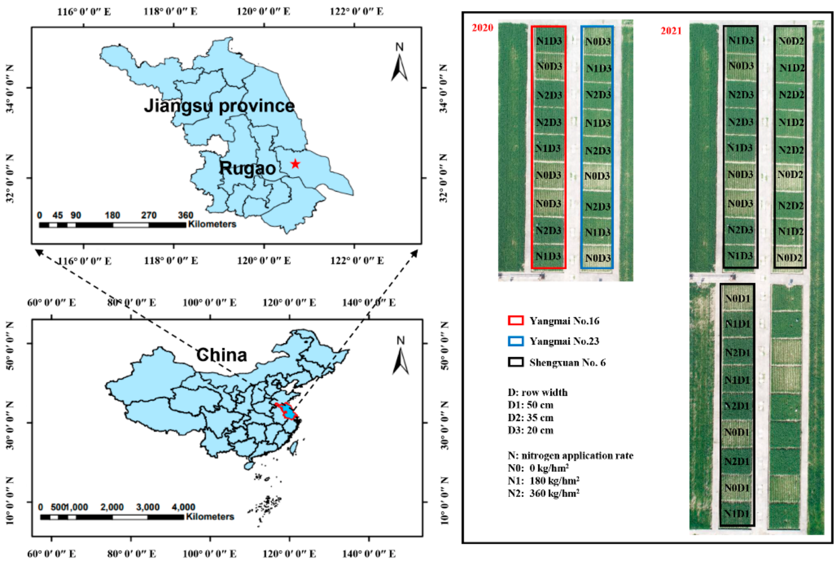
Experiment 1: This experiment was carried out in Rugao City, Jiangsu Province, China (120°45′ E, 32°16′ N) in 2020 (Figure 1). The Shengxuan No. 6 (V1) wheat variety used in this experiment has an upright plant type. Three nitrogen application rates were employed, namely 0 (N0), 180 (N1), and 360 (N2) kg/hm2. The ratio of base fertilizer to jointing fertilizer was 5:5. The base fertilizer was applied on October 27, 2019, and the jointing fertilizer was applied on March 6 2020. When the base fertilizer was applied, P2O5 (135 kg/hm2) and K2O (220 kg/hm2) were applied together. Three row widths were used, namely 50 cm (D1), 35 cm (D2), and 20 cm (D3). The test plot was 6 m long and 5 m wide, covering an area of 30 m2. The test was conducted in three growth stages of wheat, namely the jointing (S1), booting (S2), and heading (S3) stages.
Experiment 2: This experiment was carried out in Rugao, Jiangsu, China (120°45′ E, 32°16′ N) in 2021. The Yangmai No.16 (V2) and Yangmai No.23 (V3) wheat varieties used in this experiment were flat and upright plant types, respectively. The row width was 20 cm (D3). The nitrogen application rate, plot setting, and test time were the same as those in Experiment 1. The base fertilizer for Experiment 2 was applied on 30 October 2020, and the jointing fertilizer was applied on 7 March 2020.
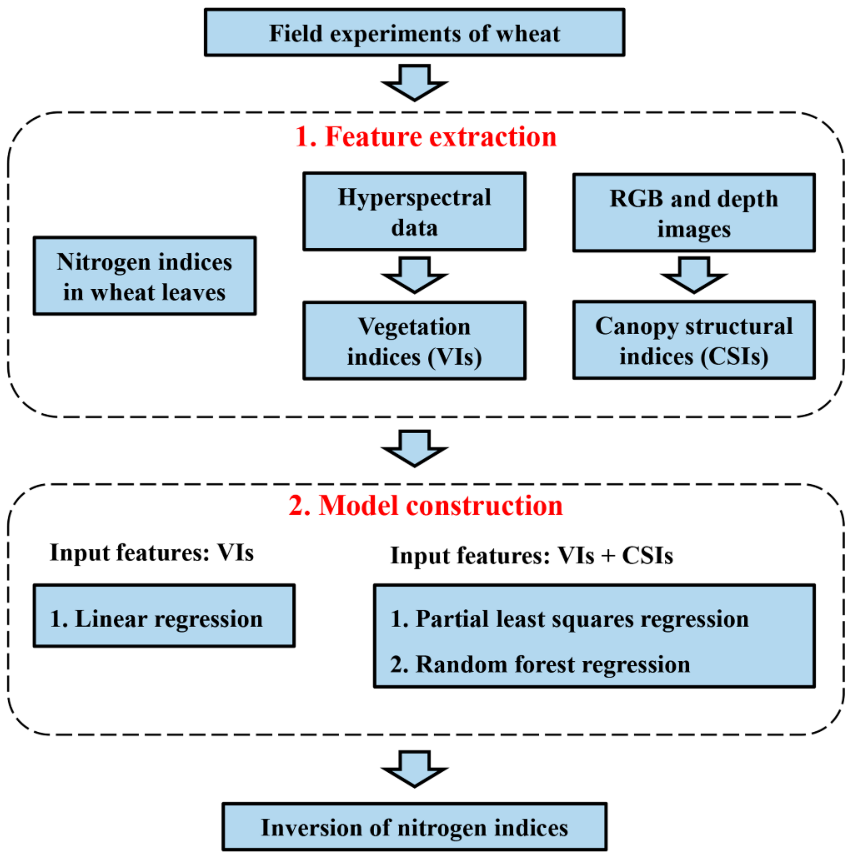
Figure 2 shows the flowchart of this research.
2.2. Data Acquisition
2.2.1. Acquisition of Spectral Data
An ASD FieldSpec Handheld 2 (Analytical Spectral Devices, Boulder, CO, USA) was used to obtain the spectral data of the wheat canopy. The spectrometer can acquire the spectral reflectance of the target at 325–1075 nm, with a wavelength accuracy of 1 nm and a field angle of 25°. The test was conducted around noon (10:30–14:00 h) on sunny days, and the spectrometer was placed 1 m away from the wheat canopy. Spectral data were collected at jointing, booting, and heading stages. Data acquisition dates for Experiment 1 were 13 March, 23 March, and 7 April, and data acquisition dates for Experiment 2 were 14 March, 20 March, and 2 April. Three sample points were randomly selected from each plot for testing, and the average value of the tested results of the three sample points was taken as the spectral data of each plot. There was a total of 135 samples of spectral data.
2.2.2. Acquisition of RGB and Depth Images
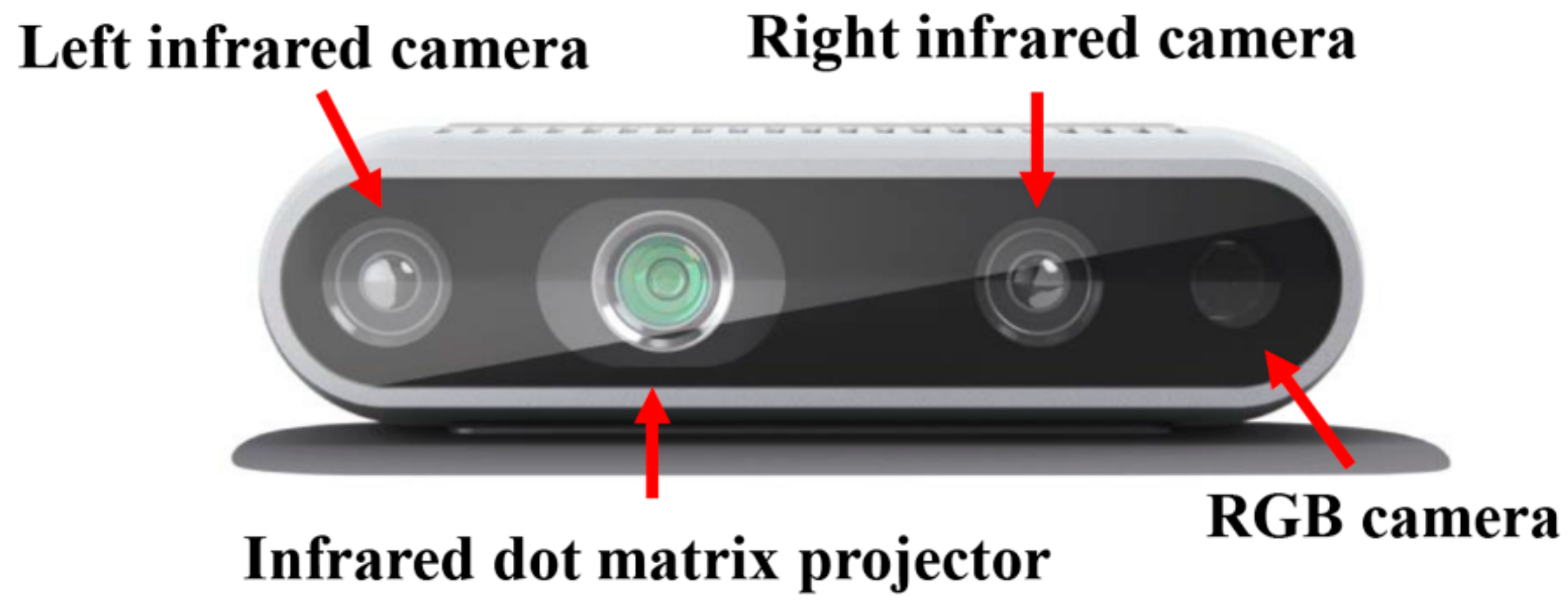
The Intel® RealSense™ Depth Camera D435i (Integrated Electronics Corporation, Santa Clara, CA, USA) captured the RGB-D images of the wheat canopy vertically from above the canopy (Figure 3). Carrying a structured light infrared projector, the camera projected light with certain structural characteristics onto the target; the special infrared camera collected different image phase information, and such structural change was then converted into depth information through the arithmetic unit. Three locations in each plot were randomly selected to acquire images, and each location acquired an RGB image and a depth image. Images were taken at 4:00 p.m. on the same date as the spectral data acquisition. The D435i had a shooting range of 0.3–10 m and a field angle of 69.4° × 42.5° × 77°. The resolution of both the depth and RGB images was 1280 × 720 pixels. To prevent the photographer’s body parts from getting into the picture, the 720 × 720 central area was used to extract the canopy structural features, and the average value of the tested results of three sample points were taken as the canopy structural features of each plot.
2.2.3. Acquisition of Agronomic Parameters
Continuous wheat plants with a row width of 50 cm were selected in each plot for destructive sampling. The above-ground organs of wheat were placed into paper bags, de-enzymed at 105 °C for 30 min and then dried at 80 °C to a constant weight. Next, the leaf dry weight (LDW) was obtained. The dried wheat leaves were ground into powder, and the LNC of the target wheat plant was obtained by the Kjeldahl method. The LNA was calculated as follows:
The plant samples’ collection time was consistent with the spectral data. The number of plant samples was also 135.
2.3. Data Analysis
2.3.1. Preprocessing of Depth Images
The depth value of each point in the depth image revealed the distance from the target to the camera plane. By subtracting the depth value of each point in the depth image from the distance from the ground to the camera plane, we obtained the height image of the canopy. However, in the actual shooting process, affected by factors such as the slope of the field, the camera plane is often not parallel to the ground. Consequently, the obtained height image cannot reflect the true height of the wheat canopy. To solve this problem, each depth image was preprocessed by the correction method proposed by Li et al. [16]. The error caused by the tilt between the camera plane and the ground was eliminated by fitting the plane where the canopy was located using the least squares method, and then estimating the tilt angle between the camera and the ground.
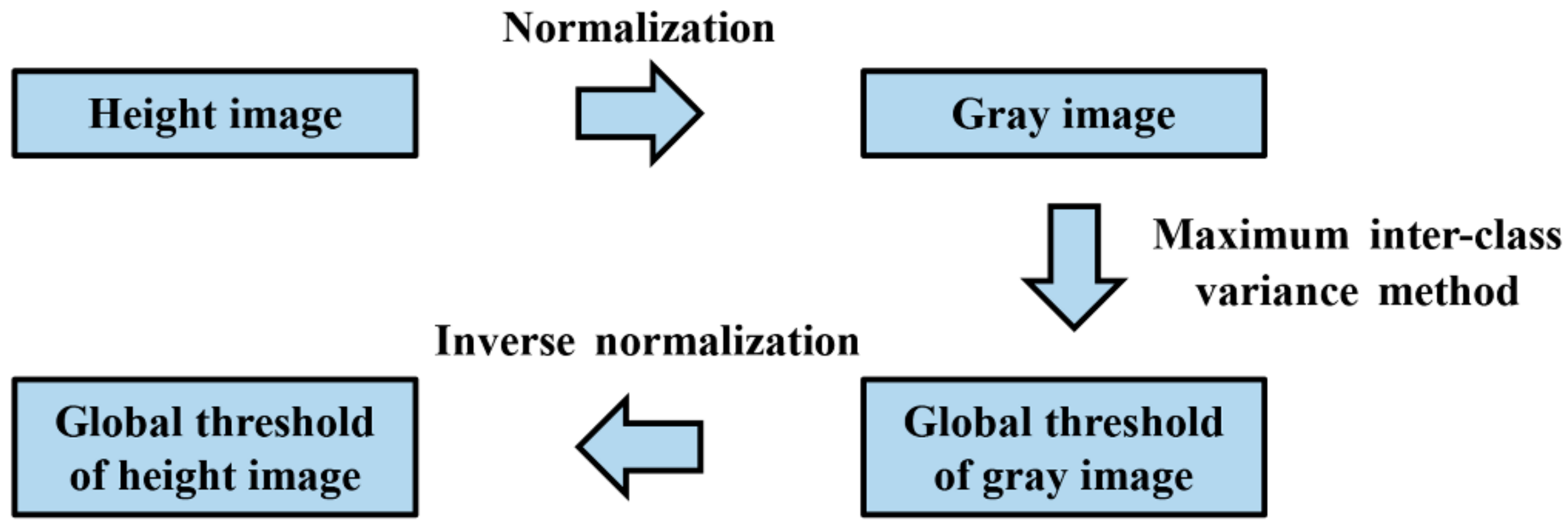
To facilitate the extraction of canopy structural features, it is necessary to segment the height image. Because the height values are uniformly distributed in the corrected height image, image segmentation can be carried out by calculating the global threshold [27]. In this study, the maximum inter-class variance method commonly used in the segmentation of gray images was applied to segment the height image (Figure 4).
2.3.2. Feature Extraction of Digital Images
The fractional vegetation cover (FVC) and canopy height features were extracted based on each preprocessed height image. In the segmented height image, the area with a height value of 0 indicates the soil background, while the area with a height value greater than 0 represents the wheat canopy. The FVC is the total number of pixels in the height image divided by the number of pixels in the wheat canopy. In this study, the canopy height features included the average height, height standard deviation, height variation coefficient, and height percentile.
The canopy textural features were extracted from the RGB images of wheat canopy. To make good use of the color information of the RGB images, the Color Co-occurrence Matrix proposed by Palm [28] based on the gray level co-occurrence matrix was used in this study to quantify the spatial correlation between different color channels and to describe the color and texture properties of the images. The obtained canopy images were transformed from the RGB color space to the hue, saturation, value color space for further processing, so as to extract four classic Haralick features, i.e., entropy (ENT), angular second moment (ASM), contrast (CON), and correlation (COR).
2.3.3. Selection of Spectral Indices
The physical meanings of LNC and LNA are very different, and their corresponding sensitive bands are also different. LNA is the nitrogen index obtained by multiplying LNC and LDW, and its value is affected by these two parameters. For LNC, nitrogen is one of the important constituent elements of chlorophyll, so the spectral characteristics of LNC and chlorophyll are similar [29]. The red and blue light bands are the absorption peaks of chlorophyll, and the reflectance of these bands is highly correlated with the chlorophyll content of leaves [6,30]. Therefore, the red and blue light bands are also sensitive to LNC. For LDW, although there is no direct relationship between this indicator and canopy structure indices such as LAI, both are affected by multiple factors such as nitrogen application rate and planting density [31,32]. Therefore, the sensitive bands of biomass and canopy structure characteristics are also similar, and both are more sensitive to the near infrared bands.
Considering the difference in spectral characteristics between LNA and LNC, two vegetation indices were selected for the inversion of LNA and LNC in this study. The first vegetation index, RVI, contains red and near-infrared bands and can accurately invert wheat LNA [9]. The second vegetation index was the Angular Insensitivity Vegetation Index (AIVI) proposed by He et al. [33] This vegetation index is very sensitive to chlorophyll and less affected by the observation angle. Li et al. [34] found that AIVI was poorly correlated with LAI, and insensitive to structural changes in the canopy. RVI and AIVI are calculated as follows:
where R660, R815, R735, R720, R573, and R445 represent the spectral reflectance at 660 nm, 815 nm, 735 nm, 720 nm, 573 nm, and 445 nm, respectively. Features obtained in this study are described in Table 1.
2.3.4. Linear Regression Model
Taking RVI and AIVI as independent variables, linear regression models were constructed based on the least squares method to predict wheat LNA and LNC. The accuracy of the models was verified by 10-fold cross validation. The data set was divided into ten subsets. For each validation, one subset was taken as the validation set, and the remaining subsets served as the training sets. The average of the ten validation results was regarded as the final value. Two indices, R2 and RMSE, were used to evaluate the performance of LNA and LNC prediction models:
where SSR and SSE denote the sum of squared residuals and the sum of squared errors, respectively; Pi and Oi denote the predicted and measured values, respectively; and n is the number of samples.
2.3.5. PLS Regression Model
A multiple linear regression method, PLS, integrates the characteristics of principal component analysis and correlation analysis. Similar to principal component regression, PLS transforms the original independent variables and dependent variables into a new linear combination (i.e., the components) before constructing a linear regression model. When creating the components, principal component regression only considers the variability of independent variables, but PLS takes the dependent variables into consideration as well. This makes PLS more suitable for regression modeling under the condition of numerous multiple correlations of independent variables. As an extended algorithm of multiple linear regression, PLS aims to establish a linear combination relationship as shown below:
where Y is a matrix with one variable (LNA or LNC) and n sample points, X is a matrix with k variables (vegetation indices and canopy structural features) and n sample points, B is a regression coefficient matrix, and E is the error matrix. The normalized X and Y were used for calculation. Principal components, c1, c2... cA, were extracted from X, and the covariance between each principal component and the dependent variables (LNA and LNC) should be maximized so as to carry as much information as possible and have the strongest interpretability for Y. On this basis, the regression equation between A principal components and X or Y was obtained as follows:
where T is the factor score matrix, W refers to the weight matrix, and Q is the regression coefficient matrix of T. By substituting Equation (7) into Equation (8), and restoring the normalized data into the original data, the PLS regression model was obtained.
The importance of different features in the PLS model was described by the variable influence on the projection (VIP) method, and the VIP was calculated as follows:
where VIPi denotes the VIP value of the jth independent variable, k represents the number of independent variables, A is the number of principal components, ca is the ath principal component, r(O, ca) is the correlation coefficient between dependent variables and the principal component, which reflects the principal component’s interpretability for O, and waj stands for the loading weight of the first component and the jth independent variable. The higher the VIP value, the more important this feature is. If each independent variable has the same explanatory effect on the dependent variable, the VIP value of all independent variables is 1. When a feature has a VIP value of greater than 1, this is generally regarded as a feature with a greater contribution. In this study, the R2, RMSE and VIP values of the results predicted by the PLS model were the average value of the results obtained by the 10-fold cross validation.
2.3.6. RF Regression Model
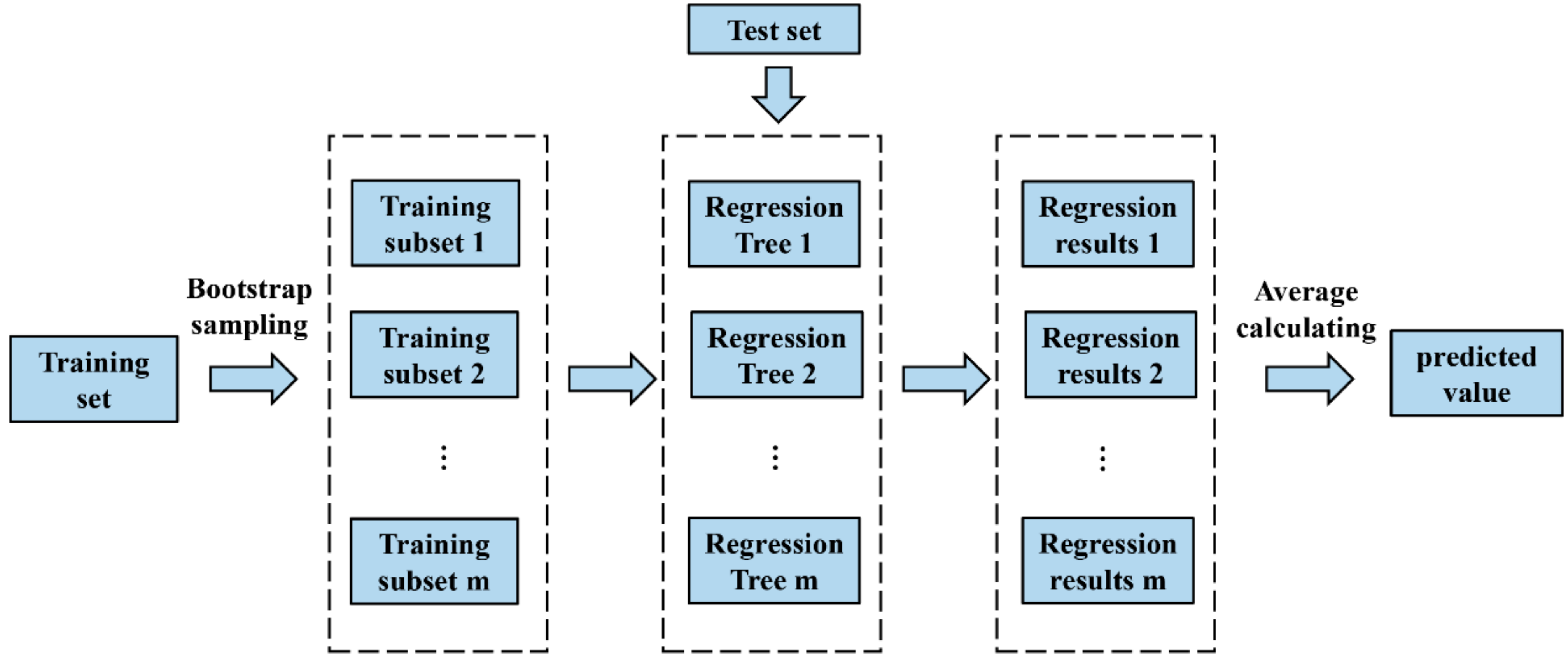
Random forest regression is an integrated learning method that is well applicable to the regression of high-dimensional data. Feature selection is not required before building the model, and the model strongly resists against overfitting. In this study, a single vegetation index and multiple canopy structural features served as the input parameters of the RF model, with LNA and LNC being the output parameters. A single regression tree was constructed as follows: the training set with n training samples was sampled, and n samples were extracted to form the input samples of a single regression tree; t features were randomly selected from the k features of the training set as the features of the regression tree (t < k); the regression tree was established by completely splitting the sampled data; that is, a leaf node could not be further split or all samples of this node output the same value. The RF regression model was randomly constructed with multiple regression trees in the modeling process, and the output value was the average of all regression trees in the model, that is, the predicted nitrogen index of the target (Figure 5).
With strong interpretability, the RF model can distinguish the degree to which different input features influence the prediction results, that is, the importance of each feature. In this study, based on the method proposed by Breiman [24] which was to analyze the importance of RF features, 30% of the data was randomly selected as the validation set and the remaining data served as the training set. The sort order of the samples of a feature was disrupted, and the rising proportion of mean square error (MSE) was used as an index for the importance of this feature. MSE was calculated as follows:
where Pi and Oi denote the predicted and measured value, respectively, and n represents the number of samples.
3. Results
3.1. Correlation Analysis
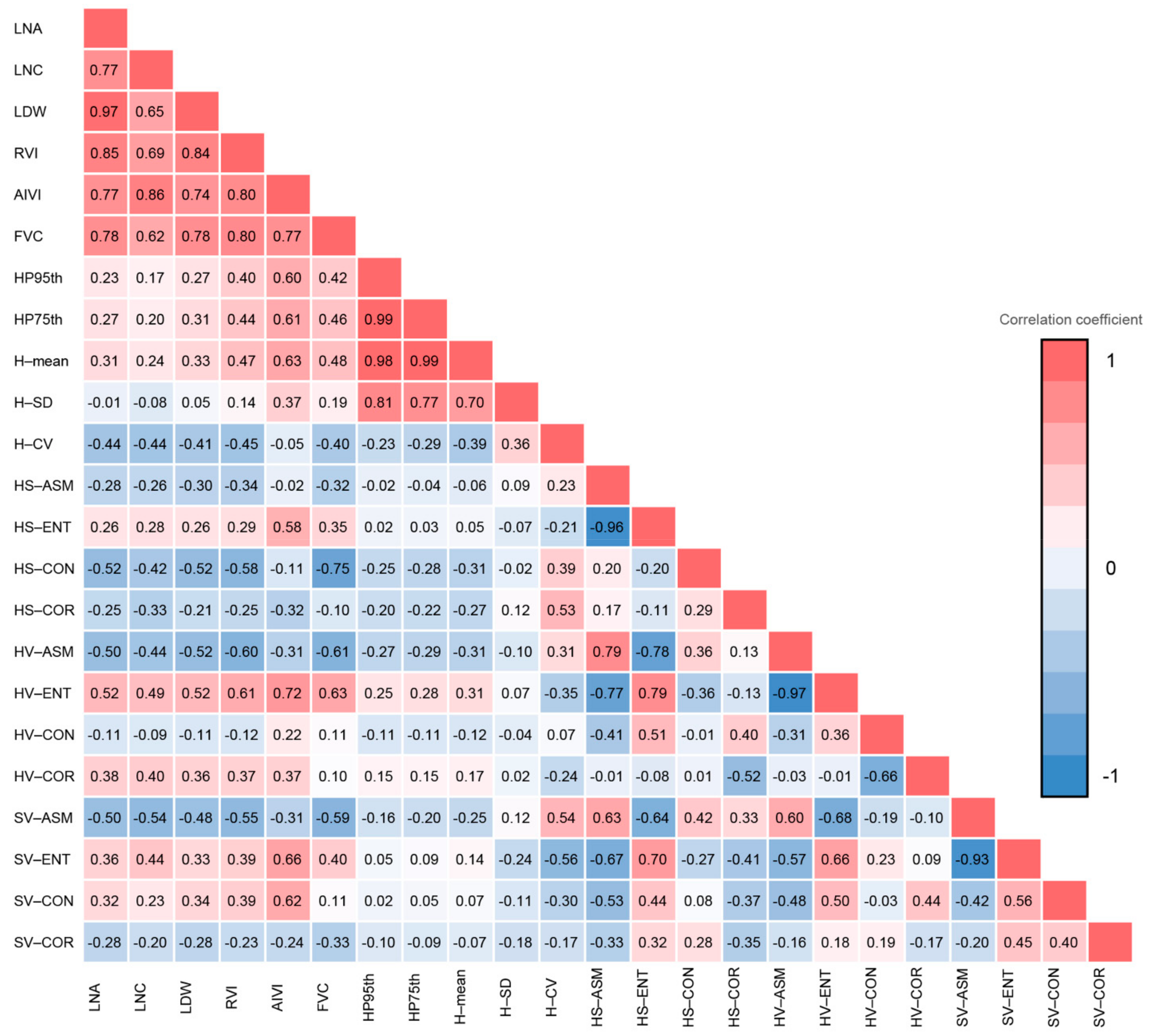
Figure 6 shows the correlation between wheat nitrogen indices, vegetation indices, and canopy structural features obtained under different nitrogen application rates, planting densities, and phenological periods. The correlation coefficient between LNA and RVI was 0.85, and that between LNA and AIVI was 0.77, while the correlation coefficient between LNC and RVI was 0.69, and that between LNC and AIVI was 0.86. This indicated that RVI was more closely correlated with LNA, and AIVI was more suitable for monitoring LNC. In addition, FVC, HS-CON, HV-ASM, and HV-ENT were the canopy structural features that were highly correlated with LNA, while features that were highly correlated with LNC included FVC and SV-ASM. Both nitrogen indices were highly correlated with FVC and some textural features, but were less correlated with height features.
The correlation between vegetation indices and canopy structural features was analyzed. The results showed that RVI was highly correlated with structural features such as FVC, HS-CON, HV-ASM, HV-ENT and SV-ASM, while AIVI was highly correlated with features such as FVC, height feature, HS-ENT, HV-ENT, SV-ENT, and SV-CON. Based on the above results, due to a strong correlation between some canopy structural features and vegetation indices, canopy structure will influence the accuracy of spectral monitoring of nitrogen status in wheat by affecting the values of vegetation indices. Besides, the multicollinearity among different features implies that the information revealed by these features overlaps markedly. Therefore, it is necessary to analyze the importance of each canopy structural feature in different algorithms, and clarify how canopy structural features improve the accuracy of spectral monitoring.
3.2. Prediction Accuracy of Different Algorithms
Table 2 shows the prediction results of models established based on different algorithms. The input parameter of the linear regression model was a single vegetation index, while the input parameters of the PLS and RF models included vegetation indices and CSIs. The results obtained by the linear regression model showed that RVI’s prediction for LNA and LNC had an R2 of 0.73 and 0.48, respectively (RMSE: 1.69 g/m2 and 0.55%, respectively). The AIVI’s prediction for LNA and LNC had an R2 of 0.68 and 0.64, respectively (RMSE: 2.02 g/m2 and 0.42%, respectively). Therefore, RVI was more suitable for the prediction of LNA only when vegetation indices were used to predict nitrogen content in wheat leaves, while AIVI was more applicable to LNC prediction.
When only CSI was used, the PLS model’s prediction for LNA and LNC had an R2 of 0.71 and 0.57, respectively (RMSE: 1.80 g/m2 and 0.48%, respectively). The RF model had an R2 of 0.76 and 0.64 for LNA and LNC, respectively (RMSE: 1.66 g/m2 and 0.43%, respectively). The RF algorithm outperformed the PLS algorithm in terms of the prediction accuracy of LNA and LNC.
When both vegetation indices and CSI were used, the prediction accuracy for LNA and LNC were substantially improved. The PLS and RF models with RVI and CSI as the inputs increased the R2 of LNA prediction to 0.78 and 0.79, respectively (RMSE: 1.58 g/m2 and 1.54 g/m2, respectively), while the R2 of LNC prediction was increased to 0.61 and 0.70, respectively (RMSE: 0.47% and 0.40%, respectively). The PLS and RF models with AIVI and CSI as the input parameters improved the R2 of LNA prediction to 0.78 and 0.75, respectively (RMSE: 1.67 g/m2 and 1.56 g/m2, respectively), while the R2 of LNC prediction was increased to 0.61 and 0.70, respectively (RMSE: 0.35% and 0.37%). Based on the above results, PLS and RF regression algorithms that integrate spectral information and canopy structural information can effectively improve the prediction accuracy of LNC and LNA. The RF model with RVI and canopy structural features had the highest prediction accuracy for LNA, while the PLS model with AIVI and canopy structural features had the highest prediction accuracy for LNC.
3.3. Importance of Features in the PLS Model
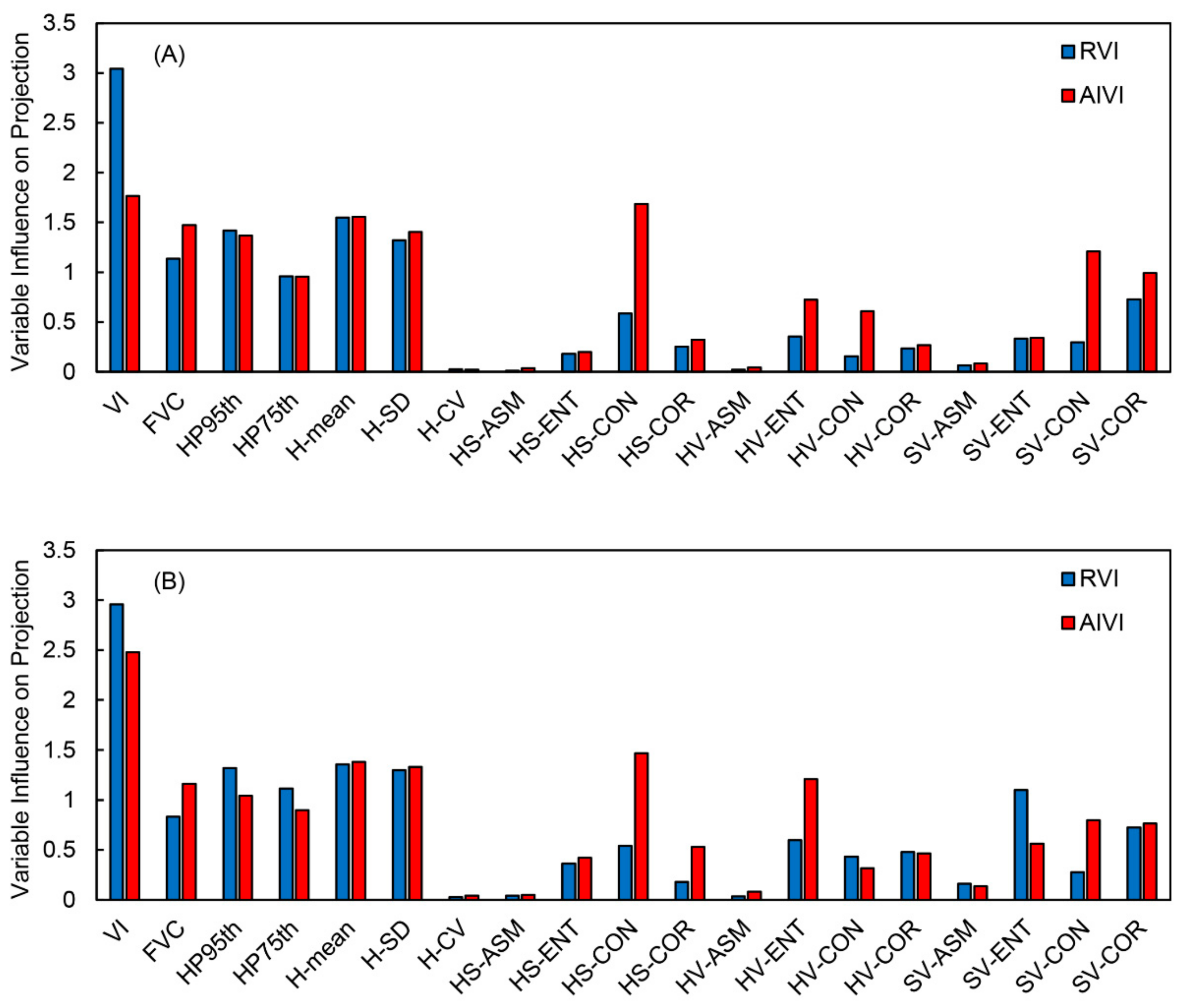
Figure 7 shows the VIP values of different features in LNA and LNC prediction models established based on the PLS algorithm. In the LNA prediction model with RVI and CSI as the input parameters, the features with a VIP value exceeding 1 were as follows: RVI (3.04), mean height (H-mean; 1.55), 95th percentiles of height (HP95th; 1.42), standard deviation of height (H-SD; 1.32), and FVC (1.14). The VIP value of RVI was much larger than that of the other parameters. In addition, the VIP values of textural features strongly correlated with LNA were all less than 1, FVC ranked fifth in terms of importance, while height features that were less correlated with LNA had higher VIP values in the model.
In the LNA prediction model with AIVI and CSI as the input parameters, the features with a VIP value greater than 1 were: AIVI (1.77), HS-CON (1.69), H-mean (1.55), FVC (1.47), H-SD (1.41), HP95th (1.37), and SV-CON (1.21). Compared with those in the LNA prediction model with RVI and CSI as the input parameters, FVC and some textural features (e.g., HS-CON and SV-CON) had higher importance.
In the LNC prediction model with RVI and CSI as the input parameters, the features with a VIP value exceeding 1 were: RVI (2.96), H-mean (1.34), HP95th (1.32), H-SD (1.30), 75th percentiles of height (HP75th; 1.11) and SV-ENT (1.10). The LNC prediction model was similar to the LNA prediction model in feature importance, yet FVC had a lower importance in the LNC prediction model, with a VIP value of 0.83, and the VIP value of SV-ENT increased to 1.10.
In the LNC prediction model with AIVI and CSI as the input parameters, the features with a VIP value exceeding 1 were: AIVI (2.48), HS-CON (1.47), H-mean (1.38), H-SD (1.33), HV-ENT (1.21), FVC (1.16) and HP95th (1.04).
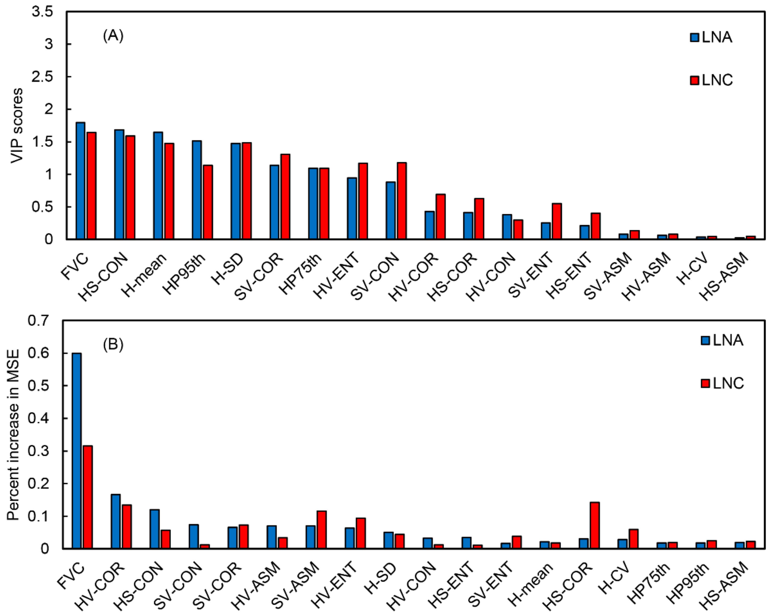
3.4. Importance of Features in RF Models
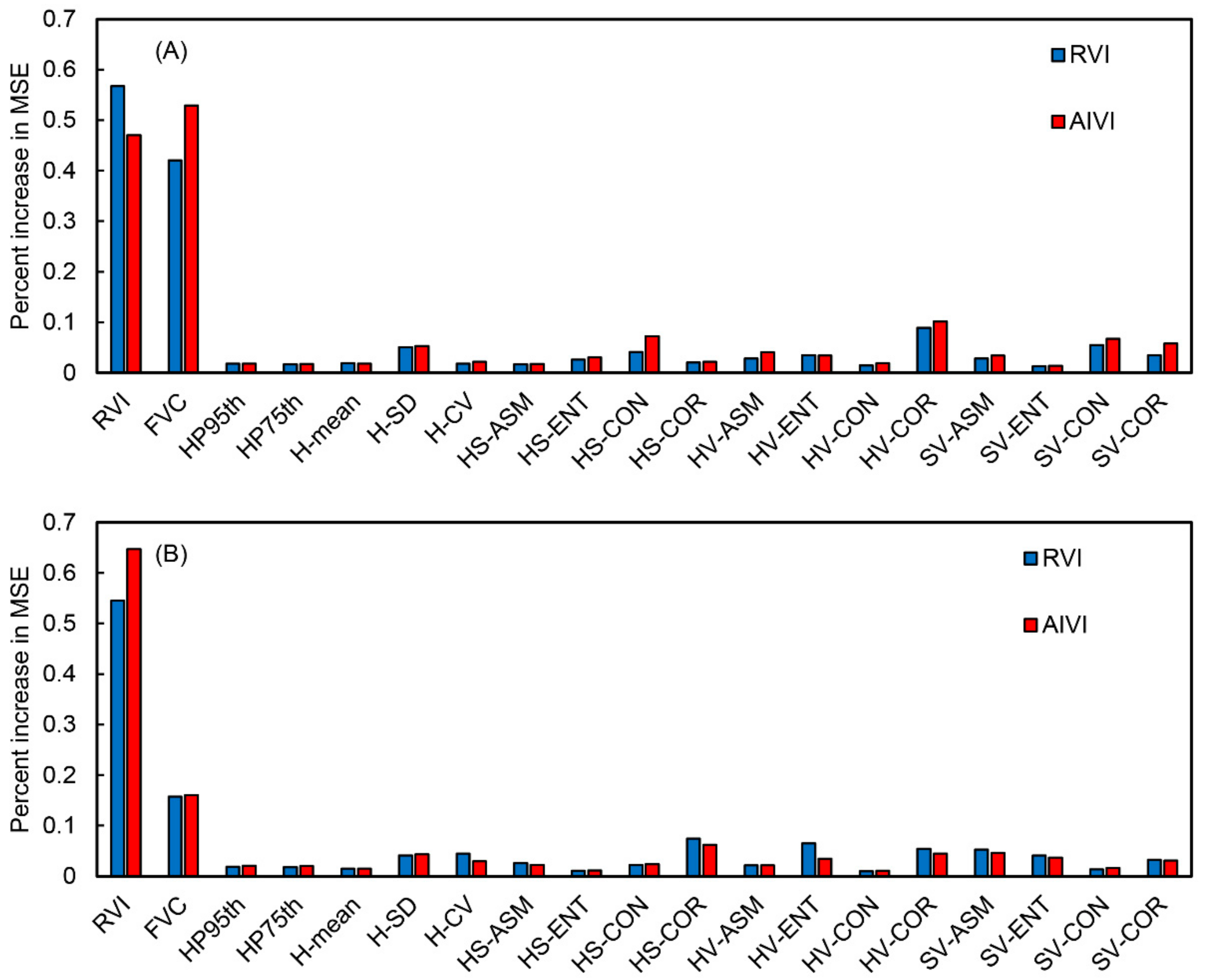
The importance of features in RF models is expressed by the percentage increase in MSE (Figure 8). In the LNA prediction model with RVI and CSI as the input parameters, with the percentage increase in MSE being 56.74% and 42.07%, RVI and FVC had much higher importance than the other parameters whose percentage increases of MSE were less than 10%. In the prediction model with AIVI and CSI as the input parameters, AIVI and FVC were more important than the other parameters, yet vegetation indices were less important than FVC, with the percentage increase in MSE reaching 47.01% and 52.89%, respectively.
In the LNC prediction model with RVI and CSI as the input parameters, the RVI maintained a high importance value, yet the importance of FVC was greatly reduced, with the percentage increase in the MSE of RVI being 54.52% and that of FVC being 15.71%. The prediction model with AIVI and CSI as the input parameters followed a similar pattern; the percentage increases in the MSE of AIVI and FVC were 64.72% and 16.01%, respectively. In addition, FVC was less important in the RF-based LNC prediction model than in the RF-based LNA prediction model, which was consistent with the results of the models established based on the PLS algorithm.
4. Discussion
4.1. Compensation of Canopy Structure Features for Vegetation Index Information
The two vegetation indices used in this study have quite different characteristics. The commonly used commercial multispectral spectrometers do not cover all the bands of these two vegetation indices. Moreover, it is difficult to extensively apply hyperspectral equipment because of its cost, which makes it hard to select the optimal vegetation indices for different monitoring targets in practical application [35,36]. Under such circumstances, the canopy structural features obtained by RGB-D cameras can effectively compensate for a lack of vegetation indices.
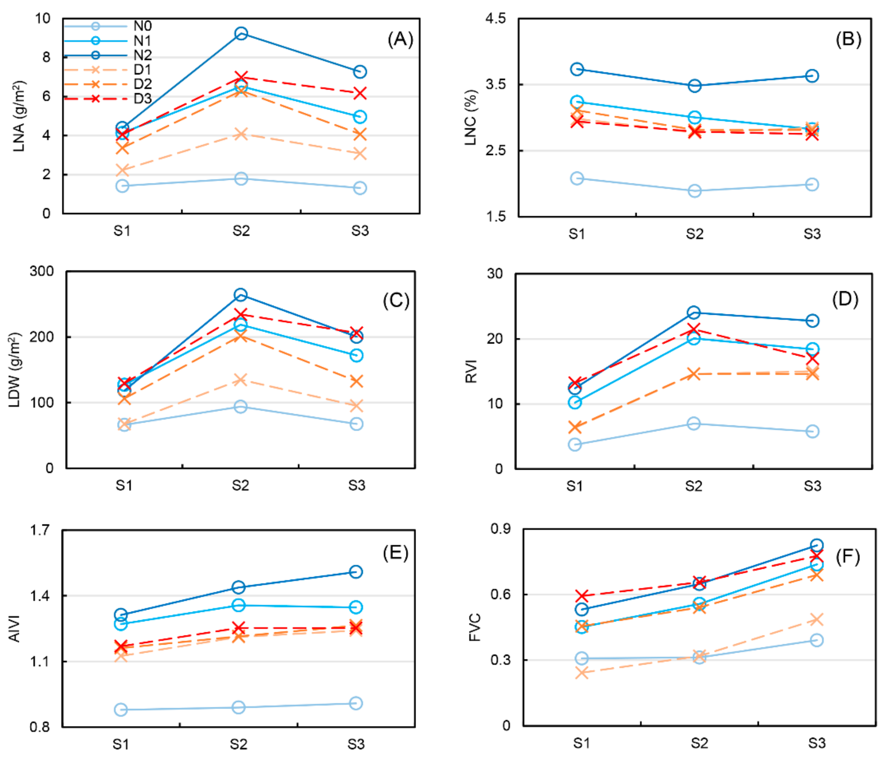
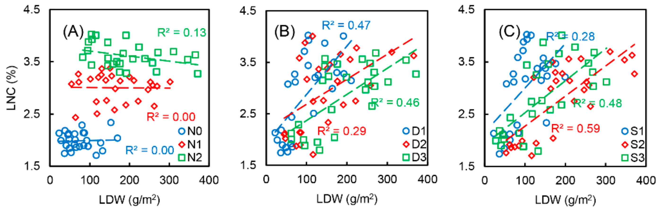
Wheat LNA and LNC are affected by factors such as nitrogen application rate, planting density and phenological period. However, their dynamic changes are not completely consistent. Nitrogen application rate has a much greater impact on LNC than planting density and phenological period, while LDW is greatly influenced by the nitrogen application rate, planting density and phenological period. As an index obtained by multiplying LNC and LDW, LNA featured a variation pattern similar to that of LDW (Figure 9). In addition, the fitting results of LNC and LDW under different nitrogen application rates, row widths, and phenological periods showed that the correlation between LNC and LDW was greatly reduced without a nitrogen application gradient (Figure 10). Hence, differences in the monitoring of LNA and LNC based on vegetation indices were mainly caused by the change in biomass that was itself dominated by planting density and phenological period.
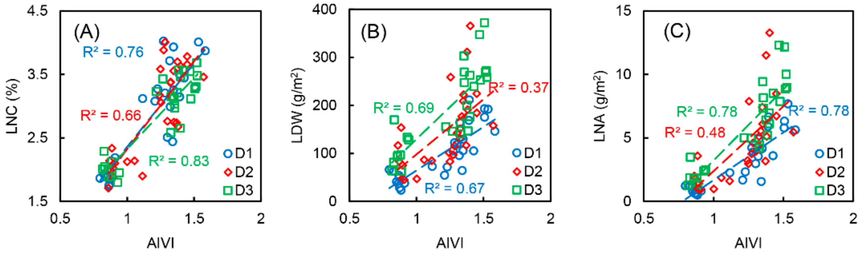
The spectral reflectance of the vegetation canopy is affected by multiple factors. External factors include sun angle and observation direction, etc., and internal factors mainly include canopy structure and physiological parameters [35,36]. On the one hand, canopy structure affects the light interception ability of vegetation, that is, under different canopy structure conditions, the ratio of reflected light between vegetation and background is different [37]. On the other hand, the scattering ability of light in the canopy under different canopy structure conditions is different, and the ratio of specular reflection and diffuse reflection is also different [38]. These reasons lead to differences in the bidirectional reflectance distribution of the crop canopy, and the reflected light has different intensities in different directions, resulting in errors in the measured spectral reflectance or vegetation index [39]. The AIVI used in this study was less affected by the observation angle, so it was sensitive to chlorophyll but insensitive to canopy structure, and its variation was relatively consistent with that of LNC. Therefore, the values of AIVI were less affected by planting density and phenological period, and the fitting curves of AIVI and LNC with different row widths were relatively similar (Figure 11). However, for LNA, AIVI lacked information about LDW, so the fitting curve of AIVI greatly differed from those of LDW and LNA under different row widths. The variation pattern of canopy structural features such as FVC was consistent with that of LNA under different row widths, which can improve the prediction accuracy of LNA by compensating for the canopy structural information missing in AIVI.
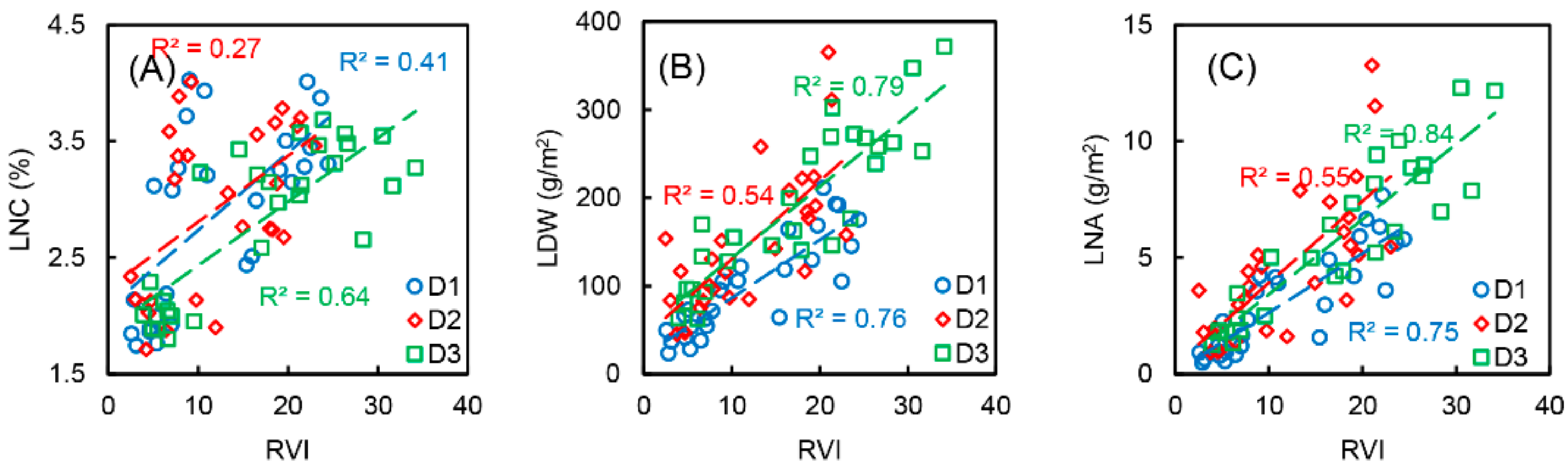
The RVI contains information about both chlorophyll and canopy structure. Changes in canopy structure caused by variations in the application rate of nitrogen, planting density, and phenological period will interfere with the numerical values of vegetation indices, resulting in different fitting curves under different conditions (Figure 12) [40]. It should be noted that under row widths D1 and D2, the RVI values were quite similar, which indicates that the influence of row width on RVI will be weakened when the row width reaches a specific threshold. This phenomenon is probably related to the field angle of the spectrometer. The ASD FieldSpec HandHeld 2 used in this study has a field angle of 25°. It was placed about 100 cm above the canopy (average distance above the ground was about 150 cm), with a field radius of about 33 cm. However, since both D1 and D2 were larger than the field radius, the vegetation indices failed to reveal the difference in row width. With a field angle larger than that of this spectrometer, the RGB-D camera can capture canopy images of wheat in multiple rows, and the extracted CSI can provide the information that the spectrometer cannot reflect, thereby improving the monitoring accuracy.
4.2. Important Features in Nitrogen Index Monitoring Modeling
The PLS and RF algorithms are characterized by strong interpretability, and thus, can be used to screen the extracted features [26]. Because the PLS model considers the collinearity between independent variables, although parameters such as FVC are strongly correlated with nitrogen index, they are not highly important in the PLS model. In the LNC and LNA prediction models established based on the PLS algorithm, vegetation indices are more important than the other parameters. However, the vegetation height feature is less affected by collinearity because of its low correlation with vegetation indices, which causes the height feature to outweigh FVC and most textural features in the model. Unlike RVI, AIVI is not significantly more important than the other parameters in the LNA prediction model. First, AIVI is less correlated with LNA when compared with RVI. Second, since AIVI is poorly correlated with FVC and textural features, multicollinearity exerts a relatively small impact on AIVI. For instance, the correlation coefficient between textural feature HS-CON and RVI is −0.58, and that between HS-CON and AIVI is −0.11. AIVI and HS-CON contain very different information; thus, HS-CON plays a greater role in compensating for AIVI than RVI.
In the prediction model established based on the RF algorithm, vegetation indices and FVC are much more important than height information and textural features. The strong correlation between FVC and vegetation indices does not affect the application of FVC in the RF-based model, which is quite different from the PLS-based model. Established PLS and RF models were used to predict the potassium content and accumulation in rice leaves based on hyperspectral data by Yang et al. [26], who found that the two models had important but inconsistent features. Meanwhile, the RF model screened out more important features than the PLS model, which was consistent with the results of the present study. Ultimately, to reduce data redundancy and ensure the prediction accuracy of the model, different features should be extracted based on the differences between the PLS and RF models in practice.
4.3. Application Potential of RGB-D Cameras
In the present study, CSI was extracted based on the RGB images and depth images captured by the RGB-D camera RealSense D435i (Integrated Electronics Corporation). The extraction of CSI has always been one of the important parts of monitoring crop growth, and it has also been the research focus of phenotypes in recent years [41,42]. Over the past few decades, a variety of remote sensing methods have been used to indirectly extract canopy structural features, and the related equipment includes RGB cameras, spectral cameras, laser radars, and fisheye sensors [43,44]. Fisheye sensors, such as the LAI-2200C canopy analyzer (LI-COR, Lincoln, NE, USA), are commonly used to extract canopy structural features, which can accurately extract multiple indices such as LAI and leaf angle [45]. However, the LAI-2200C canopy analyzer needs to be operated repetitively above and below the canopy, the operation process is relatively complicated, and it is difficult to mount it on unmanned aerial vehicles or vehicular platforms, which greatly limits it application. The RGB and spectral cameras based on the UAV platform can obtain time series crop image sets, and the three-dimensional reconstruction of crops can be realized by using motion reconstruction algorithms [46]. Although this method can effectively obtain the height characteristics of crops, it is currently mainly used in sparsely planted crops, and its application in wheat still needs to be further tested. In addition, the operation process of this method is relatively complicated, and the extraction accuracy is affected by the UAV flight height, image resolution, positioning information accuracy, etc., and its stability and universality need to be strengthened [47,48]. Laser radar is another important means to acquire canopy structural features. Many studies have used the elevation information of point clouds, yet laser radars that can be used outdoors to acquire massive amounts of data are extremely expensive, which constrains the research and application prospects of such equipment [49,50].
The application of the RGB-D camera in agriculture as a new crop phenotype monitoring device [51] has rarely been studied. In this study, the CSI obtained by the RGB-D camera served as compensation for vegetation indices, which increased the prediction accuracy of LNA and LNC in wheat. In fact, the PLS and RF models established with only CSI as the input parameter were able to accurately monitor wheat nitrogen indices, and the monitoring accuracy was higher than that of the linear regression model (Table 2). Figure 13 shows the importance of different features in the PLS and RF models established with CSI as the input parameter. Without using vegetation indices, the importance of FVC and some textural features increased measurably. Because of their strong correlation with vegetation indices, these features can be used to replace vegetation indices. Therefore, the RGB-D camera has a promising application prospect for its ability to monitor nitrogen in crops, as well as acquire a CSI.
5. Conclusions
In this study, RGB and depth images of a wheat canopy were obtained using an RGB-D camera, and canopy height, FVC, and textural features were extracted as wheat canopy structural features. Spectral indices and CSI were used to establish the LNA and LNC prediction models based on PLS and RF algorithms. The RF-based model with RVI and CSI as the input parameters had the highest prediction accuracy for wheat LNA, with R2 being 0.79 and RMSE being 1.54 g/m2. Features that have high importance in the model included vegetation indices and FVC. In contrast, the PLS-based model with AIVI and CSI as the input parameters had the highest prediction accuracy for wheat LNC, with R2 being 0.78 and RMSE being 0.35%; vegetation indices, some textural features, and height features are important features in the model. These results demonstrate that the PLS and RF regression algorithms can be used to integrate spectral and canopy structural information to effectively improve the prediction accuracy of LNA and LNC in wheat.
Author Contributions
Conceptualization, J.N. and W.C.; methodology, W.C.; software, H.L. and D.L.; validation, K.X. and X.J.; formal analysis, J.N.; investigation, H.L.; resources, J.N.; data curation, D.L.; writing—original draft preparation, H.L. and D.L.; writing—review and editing, J.N.; visualization, K.X.; supervision, X.J.; project administration, J.N.; funding acquisition, J.N. All authors have read and agreed to the published version of the manuscript.
Funding
This research was funded by National Natural Science Foundation of China [grant number 31871524], the Primary Research & Development Plan of Jiangsu Province of China [grant numbers BE2021304], and Six Talent Peaks Project in Jiangsu Province [grant number XYDXX-049].
Acknowledgments
The authors wish to thank all those who helped in this research.
Conflicts of Interest
The authors declare no conflict of interest.
References
- Ju, X.T.; Xing, G.X.; Chen, X.P.; Zhang, S.L.; Zhang, L.J.; Liu, X.J.; Cui, Z.L.; Yin, B.; Christie, P.; Zhu, Z.L. Reducing environmental risk by improving N management in intensive Chinese agricultural systems. Proc. Natl. Acad. Sci. USA 2009, 9, 3041. [Google Scholar] [CrossRef] [PubMed] [Green Version]
- Yao, X.; Ata-Ul-Karim, S.T.; Zhu, Y.; Tian, Y.; Cao, W. Development of critical nitrogen dilution curve in rice based on leaf dry matter. Eur. J. Agron. 2014, 55, 20–28. [Google Scholar] [CrossRef]
- Li, D.; Wang, X.; Zheng, H.; Zhou, K.; Yao, X.; Tian, Y.; Zhu, Y.; Cao, W.; Cheng, T. Estimation of area- and mass-based leaf nitrogen contents of wheat and rice crops from water-removed spectra using continuous wavelet analysis. Plant Methods. 2018, 14, 76. [Google Scholar] [CrossRef] [PubMed]
- Muoz, H.R.; Guevara, G.R.; Contreras, M.L.; Torres, P.I.; Prado, O.J.; Ocampo, V.R. A Review of Methods for Sensing the Nitrogen Status in Plants: Advantages, Disadvantages and Recent Advances. Sensors 2013, 13, 10823–10843. [Google Scholar]
- Ustin, S.L.; Gitelson, A.A.; Jacquemoud, S.; Schaepman, M.; Asner, G.P.; Gamon, J.A.; Zarco-Tejada, P. Retrieval of foliar information about plant pigment systems from high resolution spectroscopy. Remote Sens. Environ. 2009, 113, S67–S77. [Google Scholar] [CrossRef] [Green Version]
- Lambers, H.; III, F.S.C.; Pons, T.L. Plant Physiological Ecology; Springer: New York, NY, USA, 2008. [Google Scholar]
- Yu, K.; Li, F.; Gnyp, M.L.; Miao, Y.; Chen, X. Remotely detecting canopy nitrogen concentration and uptake of paddy rice in the Northeast China Plain. ISPRS J. Photogramm. Remote Sens. 2013, 78, 102–115. [Google Scholar] [CrossRef]
- Li, F.; Miao, Y.; Hennig, S.D.; Gnyp, M.L.; Chen, X.; Jia, L.; Bareth, G. Evaluating hyperspectral vegetation indices for estimating nitrogen concentration of winter wheat at different growth stages. Precis. Agric. 2010, 11, 335–357. [Google Scholar] [CrossRef]
- Zhu, Y.; Yao, X.; Tian, Y.; Liu, X.; Cao, W. Analysis of common canopy vegetation indices for indicating leaf nitrogen accumulations in wheat and rice. Int. J. Appl. Earth Obs. Geoinf. 2008, 10, 1–10. [Google Scholar] [CrossRef]
- Li, F.; Li, D.; Elsayed, S.; Hu, Y.; Schmidhalter, U. Using optimized three-band spectral indices to assess canopy N uptake in corn and wheat. Eur. J. Agron. 2021, 127, 126286. [Google Scholar] [CrossRef]
- Feng, W.; Yao, X.; Zhu, Y.; Tian, Y.C.; Cao, W.X. Monitoring leaf nitrogen status with hyperspectral reflectance in wheat. Eur. J. Agron. 2008, 28, 394–404. [Google Scholar] [CrossRef]
- He, L.; Zhang, H.; Zhang, Y.; Song, X.; Feng, W.; Kang, G.; Wang, C.; Guo, T. Estimating canopy leaf nitrogen concentration in winter wheat based on multi-angular hyperspectral remote sensing. Eur. J. Agron. 2016, 73, 170–185. [Google Scholar] [CrossRef]
- Knyazikhin, Y.; Schull, M.A.; Stenberg, P.; Moettus, M.; Rautiainen, M.; Yang, Y.; Marshak, A.; Carmona, P.L.; Kaufmann, R.K.; Lewis, P. Hyperspectral remote sensing of foliar nitrogen content. Proc. Natl. Acad. Sci. USA 2012, 110, E185–E192. [Google Scholar] [CrossRef] [PubMed] [Green Version]
- Combal, B.; Baret, F.; Weiss, M.; Trubuil, A.; Macé, D.; Pragnère, A.; Myneni, R.; Knyazikhin, Y.; Wang, L. Retrieval of canopy biophysical variables from bidirectional reflectance using prior information to solve the ill-posed inverse problem. Remote Sens. Environ. 2003, 84, 1–15. [Google Scholar] [CrossRef]
- Wang, W.; Nemani, R.; Hashimoto, H.; Ganguly, S.; Huang, D.; Knyazikhin, Y.; Myneni, R.; Bala, G. An Interplay between Photons, Canopy Structure, and Recollision Probability: A Review of the Spectral Invariants Theory of 3D Canopy Radiative Transfer Processes. Remote Sens. 2018, 10, 1805. [Google Scholar] [CrossRef] [Green Version]
- Li, H.; Zhang, J.; Xu, K.; Jiang, X.; Zhu, Y.; Cao, W.; Ni, E. Spectral monitoring of wheat leaf nitrogen content based on canopy structure information compensation—ScienceDirect. Comput. Electron. Agric. 2021, 190, 106434. [Google Scholar] [CrossRef]
- Yin, X.; McClure, M.A. Relationship of Corn Yield, Biomass, and Leaf Nitrogen with Normalized Difference Vegetation Index and Plant Height. Agron. J. 2013, 105, 1005–1016. [Google Scholar] [CrossRef]
- Lemaire, G.; Oosterom, E.V.; Sheehy, J.; Jeuffroy, M.H.; Massignam, A.; Rossato, L. Is crop N demand more closely related to dry matter accumulation or leaf area expansion during vegetative growth? Field Crop. Res. 2007, 100, 91–106. [Google Scholar] [CrossRef]
- Xu, M.; Liu, R.; Chen, J.M.; Liu, Y.; Huang, W. Retrieving leaf chlorophyll content using a matrix-based vegetation index combination approach. Remote Sens. Environ. 2019, 224, 60–73. [Google Scholar] [CrossRef]
- Lu, J.; Cheng, D.; Chenming, G. Combining plant height, canopy coverage and vegetation index from UAV-based RGB images to estimate leaf nitrogen concentration of summer maize. Biosyst. Eng. 2021, 202, 42–54. [Google Scholar] [CrossRef]
- Guo, J.; Zhang, J.; Xiong, S.; Zhang, Z.; Wei, Q.; Zhang, W.; Feng, W.; Ma, X. Hyperspectral assessment of leaf nitrogen accumulation for winter wheat using different regression modeling. Precis. Agric. 2021, 22, 1634–1658. [Google Scholar] [CrossRef]
- Alckmin, G.T.D.; Kooistra, L.; Rawnsley, R.; Lucieer, A. Comparing methods to estimate perennial ryegrass biomass: Canopy height and spectral vegetation indices. Precis. Agric. 2020, 22, 205–225. [Google Scholar] [CrossRef]
- Wold, S.; Sjöström, M.; Eriksson, L. PLS-regression: A basic tool of chemometrics. Chemometr. Intell. Lab. 2001, 58, 109–130. [Google Scholar] [CrossRef]
- Breiman, L. Random Forests. Mach. Learn. 2001, 45, 5–32. [Google Scholar] [CrossRef] [Green Version]
- Mehmood, T.; Liland, K.H.; Snipen, L.; Sb, S. A review of variable selection methods in Partial Least Squares Regression. Chemom. Intell. Lab. Syst. 2012, 118, 62–69. [Google Scholar] [CrossRef]
- Yang, T.; Lu, J.; Liao, F.; Qi, H.; Yao, X.; Cheng, T.; Zhu, Y.; Cao, W.; Tian, Y. Retrieving potassium levels in wheat blades using normalised spectra. Int. J. Appl. Earth Obs. Geoinf. 2021, 102, 102412. [Google Scholar] [CrossRef]
- Otsu, N. A Threshold Selection Method from Gray-Level Histogram. Automatica 1975, 11, 285–296. [Google Scholar] [CrossRef] [Green Version]
- Palm, C. Color texture classification by integrative Co-occurrence matrices. Pattern Recognit. 2004, 37, 965–976. [Google Scholar] [CrossRef]
- Clevers, J.G.P.W.; Kooistra, L. Using Hyperspectral Remote Sensing Data for Retrieving Canopy Chlorophyll and Nitrogen Content. IEEE J. Sel. Top. Appl. Earth Obs. Remote Sens. 2012, 5, 574–583. [Google Scholar] [CrossRef]
- Yang, H.; Li, F.; Hu, Y.; Yu, K. Hyperspectral indices optimization algorithms for estimating canopy nitrogen concentration in potato (Solanum tuberosum L.). Int. J. Appl. Earth Obs. Geoinf. 2021, 102, 102416. [Google Scholar] [CrossRef]
- Jiang, J.; Zhang, Z.; Cao, Q.; Liang, Y.; Krienke, B.; Tian, Y.; Zhu, Y.; Cao, W.; Liu, X. Use of an Active Canopy Sensor Mounted on an Unmanned Aerial Vehicle to Monitor the Growth and Nitrogen Status of Winter Wheat. Remote Sens. 2020, 12, 3684. [Google Scholar] [CrossRef]
- Zhang, J.; Liu, X.; Liang, Y.; Cao, Q.; Tian, Y.; Zhu, Y.; Cao, W.; Liu, X. Using a Portable Active Sensor to Monitor Growth Parameters and Predict Grain Yield of Winter Wheat. Sensors 2019, 19, 1108. [Google Scholar] [CrossRef] [PubMed] [Green Version]
- He, L.; Song, X.; Feng, W.; Guo, B.; Zhang, Y.; Wang, Y.; Wang, C.; Guo, T. Improved remote sensing of leaf nitrogen concentration in winter wheat using multi-angular hyperspectral data. Remote Sens. Environ. 2016, 174, 122–133. [Google Scholar] [CrossRef]
- Li, D.; Chen, J.M.; Zhang, X.; Yan, Y.; Zhu, J.; Zheng, H.; Zhou, K.; Yao, X.; Tian, Y.; Zhu, Y.; et al. Improved estimation of leaf chlorophyll content of row crops from canopy reflectance spectra through minimizing canopy structural effects and optimizing off-noon observation time. Remote Sens. Environ. 2020, 248, 111985. [Google Scholar] [CrossRef]
- Ni, J.; Zhang, J.; Wu, R.; Pang, F.; Zhu, Y. Development of an Apparatus for Crop-Growth Monitoring and Diagnosis. Sensors 2018, 18, 3129. [Google Scholar] [CrossRef] [PubMed] [Green Version]
- Cao, Q.; Miao, Y.; Feng, G.; Gao, X.; Li, F.; Liu, B.; Yue, S.; Cheng, S.; Ustin, S.L.; Khosla, R. Active canopy sensing of winter wheat nitrogen status: An evaluation of two sensor systems. Comput. Electron. Agric. 2015, 112, 54–67. [Google Scholar] [CrossRef]
- Chu, X.; Guo, Y.; He, J.; Yao, X.; Zhu, Y.; Cao, W.; Cheng, T.; Tian, Y. Comparison of Different Hyperspectral Vegetation Indices for Estimating Canopy Leaf Nitrogen Accumulation in Rice. Agron. J. 2014, 106, 1911–1920. [Google Scholar] [CrossRef]
- Mao, Z.; Deng, L.; Duan, F.; Li, X.; Qiao, D. Angle effects of vegetation indices and the influence on prediction of SPAD values in soybean and maize. Int. J. Appl. Earth Obs. Geoinf. 2020, 93, 102198. [Google Scholar] [CrossRef]
- Song, X.; Xu, D.; He, L.; Feng, W.; Wang, Y.; Wang, Z.; Coburn, C.A.; Guo, T. Using multi-angle hyperspectral data to monitor canopy leaf nitrogen content of wheat. Precis. Agric. 2016, 17, 721–736. [Google Scholar] [CrossRef]
- Yue, J.; Guo, W.; Yang, G.; Zhou, C.; Feng, H.; Qiao, H. Method for accurate multi-growth-stage estimation of fractional vegetation cover using unmanned aerial vehicle remote sensing. Plant Methods 2021, 17, 51. [Google Scholar] [CrossRef]
- Houle, D.; Govindaraju, D.R.; Omholt, S. Phenomics: The next challenge. Nat. Rev. Genet. 2010, 11, 855–866. [Google Scholar] [CrossRef]
- Zhao, C.; Zhang, Y.; Du, J.; Guo, X.; Fan, J. Crop Phenomics: Current Status and Perspectives. Front. Plant Sci. 2019, 10, 714. [Google Scholar] [CrossRef] [PubMed] [Green Version]
- Yi, L. LiDAR: An important tool for next-generation phenotyping technology of high potential for plant phenomics? Comput. Electron. Agric. 2015, 119, 61–73. [Google Scholar]
- Vincent, G.; Antin, C.; Laurans, M.; Heurtebize, J.; Durrieu, S.; Lavalley, C.; Dauzat, J. Mapping plant area index of tropical evergreen forest by airborne laser scanning. A cross-validation study using LAI2200 optical sensor. Remote Sens. Environ. 2017, 198, 254–266. [Google Scholar] [CrossRef]
- Farooq, T.H.; Yan, W.; Chen, X.; Shakoor, A.; Wu, P. Dynamics of canopy development of Cunninghamia lanceolata mid-age plantation in relation to foliar nitrogen and soil quality influenced by stand density. Glob. Ecol. Conserv. 2020, 24, e01209. [Google Scholar] [CrossRef]
- Li, W.; Niu, Z.; Chen, H.; Li, D.; Wu, M.; Zhao, W. Remote estimation of canopy height and aboveground biomass of maize using high-resolution stereo images from a low-cost unmanned aerial vehicle system. Ecol. Indic. 2016, 67, 637–648. [Google Scholar] [CrossRef]
- Bendig, J.; Yu, K.; Aasen, H.; Bolten, A.; Bennertz, S.; Broscheit, J.; Gnyp, M.L.; Bareth, G. Combining UAV-based plant height from crop surface models, visible, and near infrared vegetation indices for biomass monitoring in barley. Int. J. Appl. Earth Obs. Geoinf. 2015, 39, 79–87. [Google Scholar] [CrossRef]
- Han, X.; Thomasson, J.A.; Bagnall, G.C.; Pugh, N.A.; Horne, D.W.; Rooney, W.L.; Jung, J.; Chang, A.; Malambo, L.; Popescu, S.C.; et al. Measurement and Calibration of Plant-Height from Fixed-Wing UAV Images. Sensors 2018, 18, 4092. [Google Scholar] [CrossRef] [Green Version]
- Li, P.; Zhang, X.; Wang, W.; Zheng, H.; Yao, X.; Tian, Y.; Zhu, Y.; Cao, W.; Chen, Q.; Cheng, T. Estimating aboveground and organ biomass of plant canopies across the entire season of rice growth with terrestrial laser scanning. Int. J. Appl. Earth Obs. Geoinf. 2020, 91, 102132. [Google Scholar] [CrossRef]
- Guo, T.; Fang, Y.; Cheng, T.; Tian, Y.; Zhu, Y.; Chen, Q.; Qiu, X.; Yao, X. Detection of wheat height using optimized multi-scan mode of LiDAR during the entire growth stages. Comput. Electron. Agric. 2019, 165, 104959. [Google Scholar] [CrossRef]
- Kim, W.S.; Lee, D.H.; Kim, Y.J.; Kim, T.; Choi, C.H. Stereo-vision-based crop height estimation for agricultural robots. Comput. Electron. Agric. 2021, 181, 105937. [Google Scholar] [CrossRef]
Figure 1.
Location of the experimental field.

Figure 2.
Flowchart of this study.

Figure 3.
Intel® RealSense™ Depth Camera D435i.

Figure 4.
Flowchart of height image segmentation.

Figure 5.
Construction of the random forest (RF) model and flowchart of leaf nitrogen accumulation (LNA) and leaf nitrogen content (LNC) prediction.
Figure 5.
Construction of the random forest (RF) model and flowchart of leaf nitrogen accumulation (LNA) and leaf nitrogen content (LNC) prediction.

Figure 6.
Thermodynamic diagram of correlation between the nitrogen index, vegetation index and canopy structural features.
Figure 6.
Thermodynamic diagram of correlation between the nitrogen index, vegetation index and canopy structural features.

Figure 7.
Variable influence on projection (VIP) values of different input features in LNA (A) and LNC (B) models based on the PLS algorithm.
Figure 7.
Variable influence on projection (VIP) values of different input features in LNA (A) and LNC (B) models based on the PLS algorithm.

Figure 8.
VIP values of different input features in LNA (A) and LNC (B) models based on the RF algorithm.
Figure 8.
VIP values of different input features in LNA (A) and LNC (B) models based on the RF algorithm.

Figure 9.
Dynamic changes in LNA (A), LNC (B), LDW (C), RVI (D), AIVI (E) and FVC (F); S1, S2, and S3 represent the jointing stage, booting stage, and heading stage, respectively.
Figure 9.
Dynamic changes in LNA (A), LNC (B), LDW (C), RVI (D), AIVI (E) and FVC (F); S1, S2, and S3 represent the jointing stage, booting stage, and heading stage, respectively.

Figure 10.
Correlation between LDW and LNC under different nitrogen application rates (A), row widths (B) and phenological periods (C); N0, N1, and N2 represent the nitrogen application rate of 0, 180, and 360 kg/hm2, respectively; D1, D2, and D3 represent row widths of 50, 35, and 20 cm, respectively; S1, S2, and S3 represent the jointing stage, booting stage, and heading stage, respectively.

Figure 11.
Correlation of AIVI with LNC (A), LDW (B), and LNA (C) under different row widths; D1, D2, and D3 represent row widths of 50, 35, and 20 cm, respectively.
Figure 11.
Correlation of AIVI with LNC (A), LDW (B), and LNA (C) under different row widths; D1, D2, and D3 represent row widths of 50, 35, and 20 cm, respectively.

Figure 12.
Correlation of RVI with LNC (A), LDW (B), and LNA (C) under different row widths; D1, D2, and D3 represent row widths of 50, 35, and 20 cm, respectively.
Figure 12.
Correlation of RVI with LNC (A), LDW (B), and LNA (C) under different row widths; D1, D2, and D3 represent row widths of 50, 35, and 20 cm, respectively.

Figure 13.
Importance of different features in PLS (A) and RF (B) models with canopy structural features as the input features.
Figure 13.
Importance of different features in PLS (A) and RF (B) models with canopy structural features as the input features.


Table 1.
Nitrogen indices, vegetation indices and canopy structural indices obtained in this study.
| Feature | Description | |
|---|---|---|
| Nitrogen indices | LNC | Leaf nitrogen content |
| LNA | Leaf nitrogen accumulation | |
| Vegetation indices | RVI | Ratio vegetation index |
| AIVI | Angular insensitivity vegetation index | |
| Canopy structural indices (depth image) | H-mean | Mean height |
| H-SD | Standard deviation of height | |
| H-CV | Coefficient of variation of height | |
| HP95th | 95th percentiles of height | |
| HP75th | 75th percentiles of height | |
| FVC | Fractional vegetation cover | |
| Canopy structural indices (RGB image) | HS-ASM | Angular second moment in the combined space of hue and saturation |
| HS-ENT | Entropy in the combined space of hue and saturation | |
| HS-CON | Contrast in the combined space of hue and saturation | |
| HS-COR | Correlation in the combined space of hue and saturation | |
| HV-ASM | Angular second moment in the combined space of hue and value | |
| HV-ENT | Entropy in the combined space of hue and value | |
| HV-CON | Contrast in the combined space of hue and value | |
| HV-COR | Correlation in the combined space of hue and value | |
| SV-ASM | Angular second moment in the combined space of saturation and value | |
| SV-ENT | Entropy in the combined space of saturation and value | |
| SV-CON | Contrast in the combined space of saturation and value | |
| SV-COR | Correlation in the combined space of saturation and value | |
Table 2.
Prediction accuracy of different models.
| Algorithms | Input Data | LNA Retrieval | LNC Retrieval | ||
|---|---|---|---|---|---|
| R2 | RMSE (g/m2) | R2 | RMSE (%) | ||
| Linear regression | RVI | 0.73 | 1.69 | 0.48 | 0.55 |
| AIVI | 0.68 | 2.02 | 0.64 | 0.42 | |
| Partial least squares regression | RVI + CSI | 0.78 | 1.58 | 0.61 | 0.47 |
| AIVI + CSI | 0.75 | 1.67 | 0.78 | 0.35 | |
| CSI | 0.71 | 1.80 | 0.57 | 0.48 | |
| Random forest regression | RVI + CSI | 0.79 | 1.54 | 0.70 | 0.40 |
| AIVI + CSI | 0.79 | 1.56 | 0.75 | 0.37 | |
| CSI | 0.76 | 1.66 | 0.64 | 0.43 | |
Note: CSI, canopy structural indices; RMSE, root mean square error.
Publisher’s Note: MDPI stays neutral with regard to jurisdictional claims in published maps and institutional affiliations. |
© 2022 by the authors. Licensee MDPI, Basel, Switzerland. This article is an open access article distributed under the terms and conditions of the Creative Commons Attribution (CC BY) license (https://creativecommons.org/licenses/by/4.0/).
Share and Cite
MDPI and ACS Style
Li, H.; Li, D.; Xu, K.; Cao, W.; Jiang, X.; Ni, J. Monitoring of Nitrogen Indices in Wheat Leaves Based on the Integration of Spectral and Canopy Structure Information. Agronomy 2022, 12, 833. https://doi.org/10.3390/agronomy12040833
AMA Style
Li H, Li D, Xu K, Cao W, Jiang X, Ni J. Monitoring of Nitrogen Indices in Wheat Leaves Based on the Integration of Spectral and Canopy Structure Information. Agronomy. 2022; 12(4):833. https://doi.org/10.3390/agronomy12040833
Chicago/Turabian StyleLi, Huaimin, Donghang Li, Ke Xu, Weixing Cao, Xiaoping Jiang, and Jun Ni. 2022. "Monitoring of Nitrogen Indices in Wheat Leaves Based on the Integration of Spectral and Canopy Structure Information" Agronomy 12, no. 4: 833. https://doi.org/10.3390/agronomy12040833
Note that from the first issue of 2016, this journal uses article numbers instead of page numbers. See further details here.