the Creative Commons Attribution 4.0 License.
the Creative Commons Attribution 4.0 License.
 | 13 Dec 2023
Cloud top heights and aerosol columnar properties from combined EarthCARE lidar and imager observations: the AM-CTH and AM-ACD products
Anja Hünerbein
Ulla Wandinger
Nicole Docter
Sebastian Bley
David Donovan
Gerd-Jan van Zadelhoff
The Earth Cloud, Aerosol and Radiation Explorer (EarthCARE) is a combination of multiple active and passive instruments on a single platform. The Atmospheric Lidar (ATLID) provides vertical information of clouds and aerosol particles along the satellite track. In addition, the Multi-Spectral Imager (MSI) collects multi-spectral information from the visible to the infrared wavelengths over a swath width of 150 km across the track. The ATLID–MSI Column Products processor (AM-COL) described in this paper combines the high vertical resolution of the lidar along track and the horizontal resolution of the imager across track to better characterize a three-dimensional scene. ATLID Level 2a (L2a) data from the ATLID Layer Products processor (A-LAY), MSI L2a data from the MSI Cloud Products processor (M-CLD) and the MSI Aerosol Optical Thickness processor (M-AOT), and MSI Level 1c (L1c) data are used as input to produce the synergistic columnar products: the ATLID–MSI Cloud Top Height (AM-CTH) and the ATLID–MSI Aerosol Column Descriptor (AM-ACD). The coupling of ATLID (measuring at 355 nm) and MSI (at ≥670 nm) provides multi-spectral observations of the aerosol properties. In particular, the Ångström exponent from the spectral aerosol optical thickness (AOT 355/670 nm) adds valuable information for aerosol typing. The AOT across track, the Ångström exponent and the dominant aerosol type are stored in the AM-ACD product. The accurate detection of the cloud top height (CTH) with lidar is limited to the ATLID track. The difference in the CTH detected by ATLID and retrieved by MSI is calculated along track. The similarity of MSI pixels across track with those along track is used to transfer the calculated CTH difference to the entire MSI swath. In this way, the accuracy of the CTH is increased to achieve the EarthCARE mission's goal of deriving the radiative flux at the top of the atmosphere with an accuracy of 10 W m−2 for a 100 km2 snapshot view of the atmosphere. The synergistic CTH difference is stored in the AM-CTH product. The quality status is provided with the products. It depends, e.g., on day/night conditions and the presence of multiple cloud layers. The algorithm was successfully tested using the common EarthCARE test scenes. Two definitions of the CTH from the model truth cloud extinction fields are compared: an extinction-based threshold of 20 Mm−1 provides the geometric CTH, and a cloud optical thickness threshold of 0.25 describes the radiative CTH. The first CTH definition was detected with ATLID and the second one with MSI. The geometric CTH is always higher than or equal to the radiative CTH.
- Article
(12899 KB) - Full-text XML
- BibTeX
- EndNote


Clouds and aerosol particles have a major influence on the radiation budget of the Earth as they interact with incoming solar radiation and outgoing terrestrial radiation. However, their global distribution is highly variable in time and space. Additionally, their vertical distribution is essential for accurately calculating their role in the radiation budget. The Earth Cloud, Aerosol and Radiation Explorer (EarthCARE) mission was designed (Illingworth et al., 2015) to improve global observation capabilities and radiation models. The European Space Agency (ESA) and the Japan Aerospace Exploration Agency (JAXA) built a satellite with four instruments on a single platform: a cloud-profiling radar (CPR), an atmospheric lidar (ATLID), a multi-spectral imager (MSI) and a broadband radiometer (BBR) (Illingworth et al., 2015; Wehr et al., 2023). The innovation of having two active (CPR, ATLID) and two passive (MSI, BBR) instruments on a single platform enables a highly synergistic approach in characterizing the state of the atmosphere. It is an unprecedented observational setup which will offer novel opportunities in atmospheric research beyond the initial mission goals. CPR, ATLID and MSI are used to retrieve three-dimensional (3D) scenes (e.g., Qu et al., 2023a; Mason et al., 2023b) to calculate radiative fluxes which are compared to the radiometer (BBR) measurements on board. The European and Canadian EarthCARE processing chain is presented by Eisinger et al. (2023). The need to derive the radiative flux at the top of the atmosphere with an accuracy of 10 W m−2 for a 100 km2 snapshot view of the atmosphere is the leading idea for the EarthCARE mission requirements (MRD, 2006). The vertical profiles of cloud and aerosol layers along the satellite track are provided by the active instruments ATLID and CPR (e.g., van Zadelhoff et al., 2023; Donovan et al., 2023a; Kollias et al., 2023; Irbah et al., 2023). In order to get information about the scene around the satellite track, the passive imager MSI, which provides columnar observations over a 150 km wide swath, is necessary (Docter et al., 2023; Hünerbein et al., 2023b, a). The idea of combining the vertical information from ATLID along track (“curtain”) with the columnar information from MSI along and across track (“carpet”) is illustrated in Fig. 1. This combination is an important step in the synergistic approach of EarthCARE, especially with respect to estimating the cloud top height (CTH) of optically thin clouds and assessing the aerosol type for the entire scene. The high-spectral-resolution lidar ATLID (do Carmo et al., 2021) operates at a wavelength of 355 nm with a vertical resolution of approximately 100 m below an altitude of 20 km and 500 m above 20 km. It provides vertical profiles along the satellite track of the particle backscatter and extinction coefficients, the lidar ratio, and the particle linear depolarization ratio, which are stored in the ATLID L2a product A-EBD (ATLID Extinction, Backscatter, Depolarization; Donovan et al., 2023a). The multi-spectral imager MSI measures the radiances in the visible, near-infrared and infrared (central wavelengths: 0.67, 0.865, 1.65, 2.21, 8.8, 10.8, 12.0 µm) with a 500 m spatial resolution over a swath width of 150 km across track. Combinations of these wavelengths are used to derive a cloud mask, which is provided in the MSI Cloud Mask product (M-CM; Hünerbein et al., 2023b), and to retrieve cloud optical properties such as the cloud optical thickness (COT), CTH and the effective radius of the cloud droplets, which are provided in the MSI Cloud Optical and Physical product (M-COP; Hünerbein et al., 2023a). Aerosol products, such as the aerosol optical thickness, are retrieved for the cloud-free pixels and are stored in the MSI Aerosol Optical Thickness product (M-AOT; Docter et al., 2023).
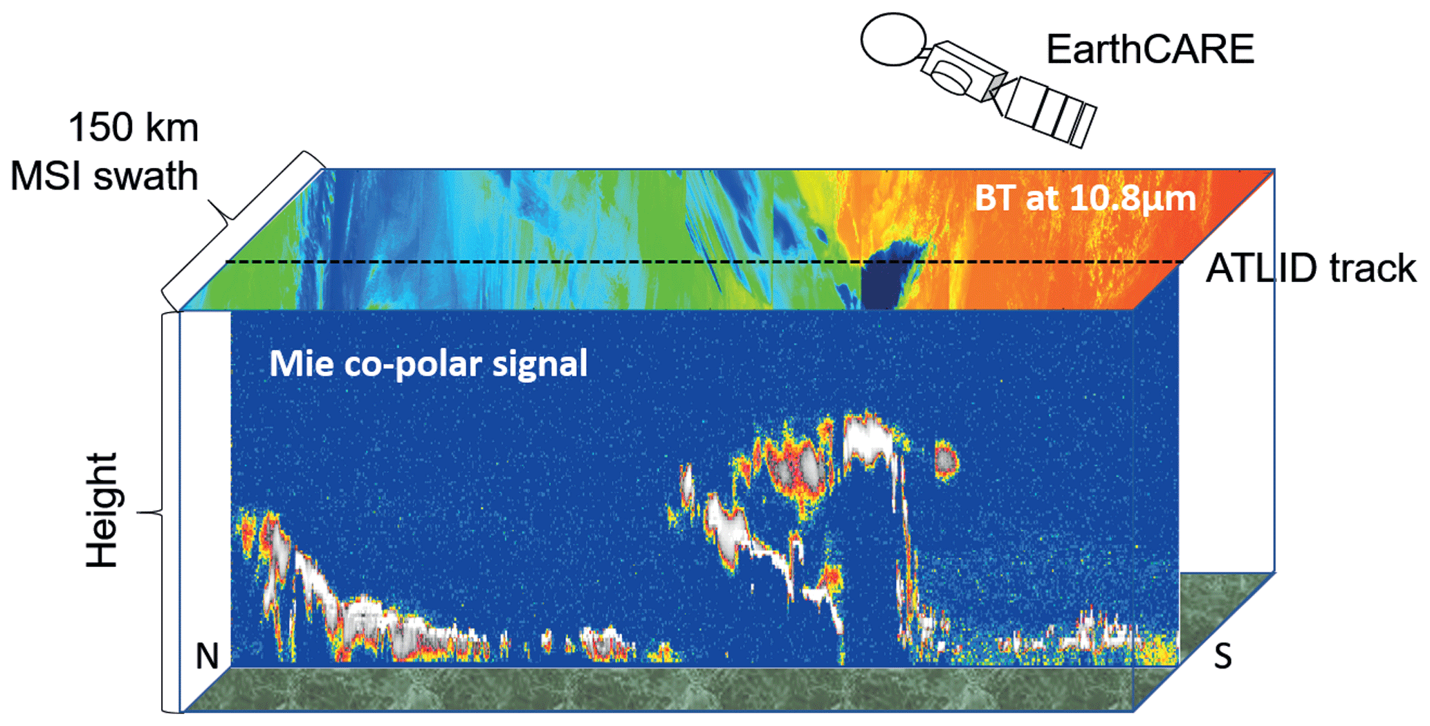
Figure 1Combined view of ATLID (curtain) and MSI (carpet) on the simulated so-called Halifax scene. A strong ATLID Mie co-polar signal (white) indicates optically thick clouds; weaker signals (red to yellow) indicate optically thinner clouds or aerosol layers. The high clouds in the center of the scene are detected by MSI on the basis of their low brightness temperature (BT; blue). The high brightness temperatures (red) on the MSI swath result from the surface return where the low broken clouds are visible in yellow.
Regarding clouds, an accuracy of the CTH for ice and water clouds of 300 m is required (mission requirements) for a 3D scene. Such accuracy cannot be achieved with MSI retrievals alone. The MSI CTH retrieval (Hünerbein et al., 2023a) is based on the measured radiation at 10.8 µm, which is thermally emitted by clouds (Fritz and Winston, 1962; Smith and Platt, 1978; Wielicki and Coakley, 1981), and gives an infrared effective radiative height. The method provides reasonable estimates for the CTH for optically thick clouds, but in the case of semi-transparent cloudiness the direct use of the measured brightness temperature will lead to a significant underestimation of the true CTH. On the other hand, ATLID can provide the physical boundaries of the cloud with the required accuracy (A-CTH product, Wandinger et al., 2023b) but only for an atmospheric cross section along track. Therefore, an algorithm for a synergistic ATLID–MSI CTH product (AM-CTH) is developed and described in the present paper. The AM-CTH product is based on the systematic investigation and classification of differences in the CTH obtained with ATLID and MSI along track. A scene classification scheme is developed to extrapolate the CTH difference to the MSI swath.
With respect to aerosol, the mission requirements demand the identification of the presence of absorbing and non-absorbing aerosol particles from natural and anthropogenic sources. Vertically resolved aerosol typing is provided along track by the ATLID Target Classification (A-TC; Irbah et al., 2023). These aerosol types weighted by the extinction coefficient of the respective height level are integrated to a column aerosol mixture in the ATLID Aerosol Layer Descriptor (A-ALD; Wandinger et al., 2023b). The M-AOT algorithm provides aerosol mixing ratios retrieved from MSI observations. The most robust way to compare the ATLID- and MSI-retrieved aerosol mixing ratios is the comparison of the dominant aerosol type, which is done in the ATLID–MSI Aerosol Column Descriptor (AM-ACD) algorithm. The Ångström exponent calculated from the ATLID observations at 355 nm and the MSI retrievals at wavelengths ≥670 nm (Docter et al., 2023) further constraints the aerosol typing because the spectral behavior contains information about the particle size. The AM-ACD product contains information on the spectral AOT, respective Ångström exponents and an estimate of the aerosol type.
AM-COL extends the ATLID information over the entire swath as long as a swath pixel can be related to a track pixel. A more sophisticated approach including radiative transfer simulations is used for the pixels close to the track in the ACM-3D product (Qu et al., 2023a). They prepare the data for the 100 km2 snapshot (20 km along track × 5 km across track), which will be used for the radiative closure. These simulations can be done for 2 pixels in each direction from the track but not for the entire swath. The AM-COL processor does not construct a 3D scene but will provide the CTH and columnar aerosol products (2D horizontally like a carpet) for the entire MSI swath width of 150 km.
The paper is structured as follows. Section 2 provides an overview of previous efforts in combining active and passive remote sensing for the determination of the CTH and for aerosol typing. A detailed description of the underlying AM-COL algorithms is provided in Sect. 3. The algorithm is validated using common test scenes from the EarthCARE end-to-end simulator (Donovan et al., 2023b) in Sect. 4. Cloud and aerosol products are always treated separately. Major findings are summarized in the Conclusions.
The combination of active and passive remote-sensing techniques on board the EarthCARE satellite is essential for reaching the mission's goal of deriving the radiative flux at the top of the atmosphere with an accuracy of 10 W m−2 for a 100 km2 snapshot view of the atmosphere. In this context, the accuracy of the CTH over the MSI swath as well as the imager-based aerosol typing need further discussion. This section intends to provide an overview of the current state of research on these two topics.
2.1 Improving passive CTH retrievals by active remote sensing
The CTH is detected from space by active and passive remote sensing. Passive retrievals use for example the MODerate resolution Imaging Spectroradiometer (MODIS), the Spinning Enhanced Visible and InfraRed Imager (SEVIRI), and the TROPOspheric Monitoring Instrument (TROPOMI; Loyola et al., 2018) on board the Sentinel-5 Precursor mission or in the near future the Plankton, Aerosol, Cloud, ocean Ecosystem mission (PACE; Sayer et al., 2023). Active measurements are taken with lidars as for example from the Cloud-Aerosol Lidar and Infrared Pathfinder Satellite Observations (CALIPSO). Active remote sensing has a high vertical resolution in detecting the geometrical CTH but is limited to observations along the narrow satellite track. Passive remote-sensing techniques offer a wider spatial coverage but with limited vertical accuracy.
From the literature it is known that CTH retrievals from passive sensors can be highly erroneous. Comparisons with lidar measurements showed large discrepancies depending on the type, height and optical thickness of the clouds. The first spaceborne comparisons of CTH detection with passive and active sensors were presented by Mahesh et al. (2004) and Naud et al. (2005). These authors used lidar observations from the Geoscience Laser Altimeter System (GLAS) to assess CTH accuracy for MODIS (aboard Terra and Aqua) and SEVIRI (aboard Meteosat-8). Besides discrepancies in the cloud mask, especially over polar regions and for optically thin clouds, they observed that the passive instruments overestimate the top height of low and opaque clouds by 0.3–0.4 km and underestimate the CTH of high and optically thin clouds. Further comparison studies (Weisz et al., 2007; Holz et al., 2008; Minnis et al., 2008; Yao et al., 2013; Iwabuchi et al., 2016; Compernolle et al., 2021) have reported different biases depending on geographical region, cloud type and altitude. Major improvements to the passive retrievals were achieved by MODIS Collection 6 (Baum et al., 2012). ESA's Cloud Climate Change Initiative has resulted in a comprehensive overview of state-of-the-art retrievals of cloud properties from passive sensors, presented in Stengel et al. (2015). A very detailed study with wide spatial coverage was performed by Mitra et al. (2021). They investigated the bias of Terra-MODIS between 50∘ S and 50∘ N against the Cloud-Aerosol Transport System (CATS) space lidar (Yorks et al., 2016) for various altitude and cloud optical thickness (COT) ranges. In the case of high clouds (CTH >5 km, defined by CATS), the bias (MODIS–CATS) was found to be −1.16 km (with a precision of 1.08 km), and for low clouds (<5 km) the bias was 40±730 m. For low clouds in particular, the bias strongly depends on COT: optically thin (COT <0.8) low clouds showed a negative bias of m, whereas optically thick (COT >0.8) low clouds were found to have a positive bias of m. For high clouds, the bias reduces with increasing COT to −280 m for COT >0.8. The presence of multi-layer clouds increases the bias between the active and passive detection of CTH ( km, Mitra et al., 2021).
Special care has to be taken in the presence of low-level clouds in the Arctic, which under certain conditions are detected with an imager but not from a space lidar (Chan and Comiso, 2011). These clouds are frequently observed in summer (Griesche et al., 2020) and are hardly visible to ground-based cloud radars because of their low altitude. Further challenges for passive CTH detection occur in the presence of thick dust layers (e.g., Robbins et al., 2022). Thus, a proper aerosol–cloud discrimination is essential.
New algorithms use machine learning or neuronal networks to obtain the CTH from passive sensors (e.g., Håkansson et al., 2018; Min et al., 2020). These algorithms are trained on previous datasets using CALIPSO. As a recent example, Tan et al. (2022) published an algorithm to assess the CTH of overlapping clouds from the Advanced Himawari Imager (AHI). Their machine-learning approach uses the available information on cloud phase, COT and neighboring cloud pixels to estimate the CTH of water and overlaying ice clouds. In a validation against CloudSat and CALIPSO, the algorithm of Tan et al. (2022) led to a reduction in the mean CTH bias from −5.1 to −2.6 km.
2.2 Aerosol typing from combined active and passive remote sensing
Besides the knowledge about the aerosol optical thickness (AOT) and the aerosol layer heights, a correct aerosol typing is essential for radiative transfer calculations. The radiative properties of an aerosol layer depend on the aerosol type or mixture. In the case of EarthCARE, the Hybrid End-To-End Aerosol Classification model (HETEAC; Wandinger et al., 2023a) is the underlying aerosol model linking the optical, microphysical and radiative properties of aerosol mixtures.
Aerosol classification schemes from active remote-sensing observations are based on the observed (intensive) optical properties. In the case of lidar measurements, the particle linear depolarization ratio (measure of particles' non-sphericity) and the extinction to backscatter ratio (lidar ratio) are the main quantities used in aerosol classification schemes (e.g., Burton et al., 2012; Groß et al., 2015). A comprehensive database of these intensive optical properties at 355 and 532 nm was collected by Floutsi et al. (2023). The CALIPSO aerosol classification scheme (Omar et al., 2009; Kim et al., 2018) could not use the lidar ratio as input because there is no direct measurement of the extinction coefficient. In contrast to CALIPSO, EarthCARE will carry a high-spectral-resolution lidar (HSRL), which provides independent measurements of the particle extinction and backscatter coefficients (at 355 nm) and therefore enables an improved aerosol classification. The first HSRL system operated successfully in space was the lidar on board ESA's wind lidar mission Aeolus (Stoffelen et al., 2005), which enabled the independent measurement of the extinction coefficient (Ansmann et al., 2007; Flament et al., 2021). In the case of multi-wavelength observations, the Ångström exponent provides additional information about the particle size. A vertically resolved aerosol typing is only possible with active remote-sensing instrumentation.
Passive remote-sensing techniques use multiple wavelengths to retrieve the AOT. From these AOT observations and the related Ångström exponents, the columnar aerosol type is determined (e.g., Toledano et al., 2007; Holzer-Popp et al., 2013; de Leeuw et al., 2015). Including polarization measurements (e.g., Russell et al., 2014) or trace-gas column densities (Penning de Vries et al., 2015) provides additional information to improve aerosol typing. In contrast to the Ångström exponent or the polarization, the AOT is an extensive property and is therefore not intrinsic to a certain aerosol type.
The ATLID–MSI Column Products processor (AM-COL) produces the ATLID–MSI Cloud Top Height (AM-CTH) product and the ATLID–MSI Aerosol Column Descriptor (AM-ACD) product. These products belong to the EarthCARE L2b products defined in the ESA EarthCARE production model and product list (Wehr et al., 2023; Eisinger et al., 2023). Since their generation requires input from ATLID L2a products created in the ATLID Layer Products processor (A-LAY; Wandinger et al., 2023b) and MSI L2a products created in the MSI Cloud Products processor and the MSI Aerosol Optical Thickness processor (M-CLD and M-AOT; Hünerbein et al., 2023b, a; Docter et al., 2023), they are produced after the ATLID L2a and MSI L2a processing is completed. An overview of the main input and output parameters and the respective products in which they are contained is provided for the cloud products in Table 1 and for the aerosol products in Table 2.
Wandinger et al., 2023bHünerbein et al., 2023bHünerbein et al., 2023aTable 1The main input and output parameters for the ATLID–MSI Cloud Top Height product and the products in which they are contained. Dimensions: X – along track, Y – across track.
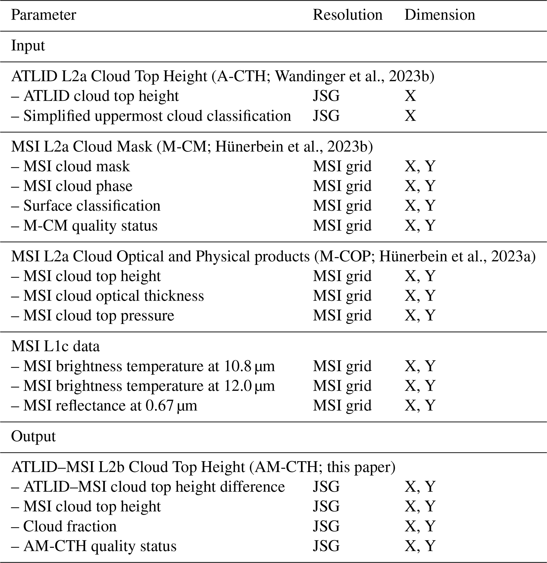
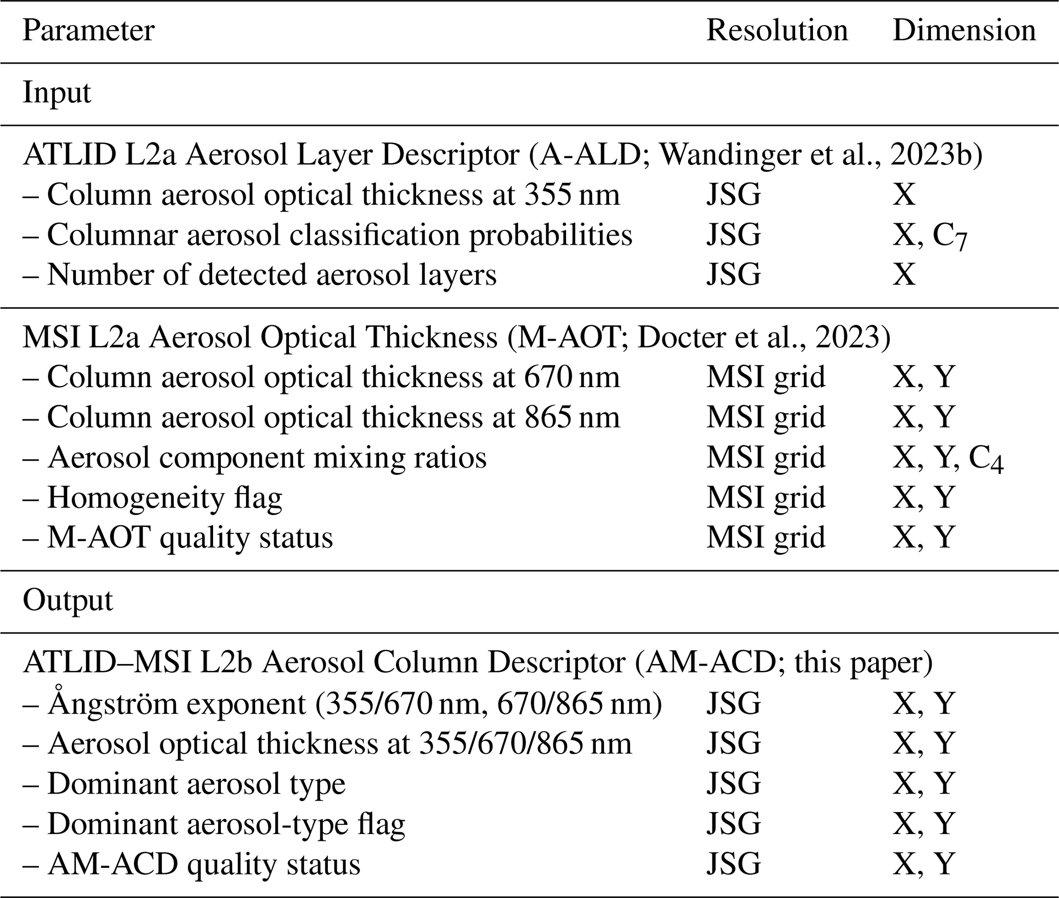
Table 2The main input and output parameters for the ATLID–MSI Aerosol Column Descriptor product and the products (with references) in which they are contained. Dimensions: X – along track, Y – across track, C4 – MSI aerosol components, C7 – ATLID aerosol types.
All calculations within the AM-COL processor are performed for one grid cell horizontal resolution on the EarthCARE Joint Standard Grid (JSG). The A-LAY products (A-CTH and A-ALD) are already provided on JSG with this resolution (approximately 1 km) along track (see Tables 1 and 2). The MSI products (M-CM, M-COP and M-AOT) are provided on the finer resolution of the MSI grid (500 m). Thus, a re-sampling is necessary, which is illustrated in Fig. 2a. First, for each JSG pixel the nearest neighbor is searched on the MSI grid. The surrounding 9 MSI pixels correspond to 1 JSG pixel. A cloud fraction for each JSG pixel is calculated from the contributing MSI pixels. Only if all contributing MSI grid cells are categorized as cloud-free (cloud fraction of 0 %) or cloudy (cloud fraction of 100 %) is the corresponding JSG pixel set to cloud-free or cloudy, respectively. The cloud mask for the MSI swath is provided in the M-CM product, and it is based on threshold tests on brightness temperatures and reflectances of individual MSI channels (Hünerbein et al., 2023b).
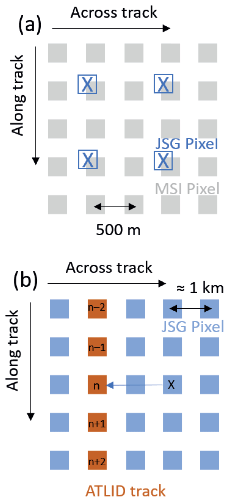
Figure 2(a) The diagram illustrates the mapping of the MSI grid to JSG. A nearest-neighbor search is implemented to link a JSG pixel to the closest MSI pixel. Usually, 9 MSI pixels correspond to 1 JSG pixel. (b) The diagram illustrates the transfer of the CTH difference from the track to the swath. For an across-track pixel, first the nearest along-track pixel is compared (five or three criteria; see Fig. 3). If no agreement is found, the search continues, alternating north (n−1) and south (n+1) of the closest along-track pixel until agreement is found or a configurable maximum search distance is reached. Then, the process is repeated for the next across-track pixel.
The AM-COL processor is split in the cloud processing algorithm AM-CTH (Sect. 3.1) applied to all cloudy pixels and the aerosol processing algorithm AM-ACD (Sect. 3.2) applied to all cloud-free pixels. Aerosol layers above or below cloud layers are not considered.
3.1 ATLID–MSI Cloud Top Height (AM-CTH) algorithm
A flowchart of the ATLID–MSI Cloud Top Height (AM-CTH) algorithm is presented in Fig. 3. It is applied to all JSG pixels considered clouds (cloud fraction of 100 %) based on the MSI cloud mask. The main output of the AM-CTH processor is the CTH difference between ATLID and MSI. The ATLID CTH was determined using the wavelet covariance transform method with thresholds from the ATLID Mie co-polar signal (Wandinger et al., 2023b). The MSI CTH provided in the M-COP product was retrieved from an optimal-estimation-based algorithm using the visible, near-infrared and thermal infrared MSI measurements (Hünerbein et al., 2023a).
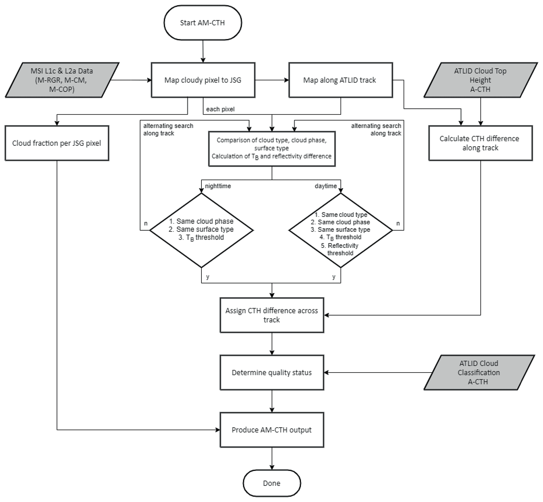
Figure 3Flowchart of the ATLID–MSI Cloud Top Height (AM-CTH) algorithm. The algorithm is applied to all cloudy JSG pixels. TB stands for brightness temperature at 10.8 µm.
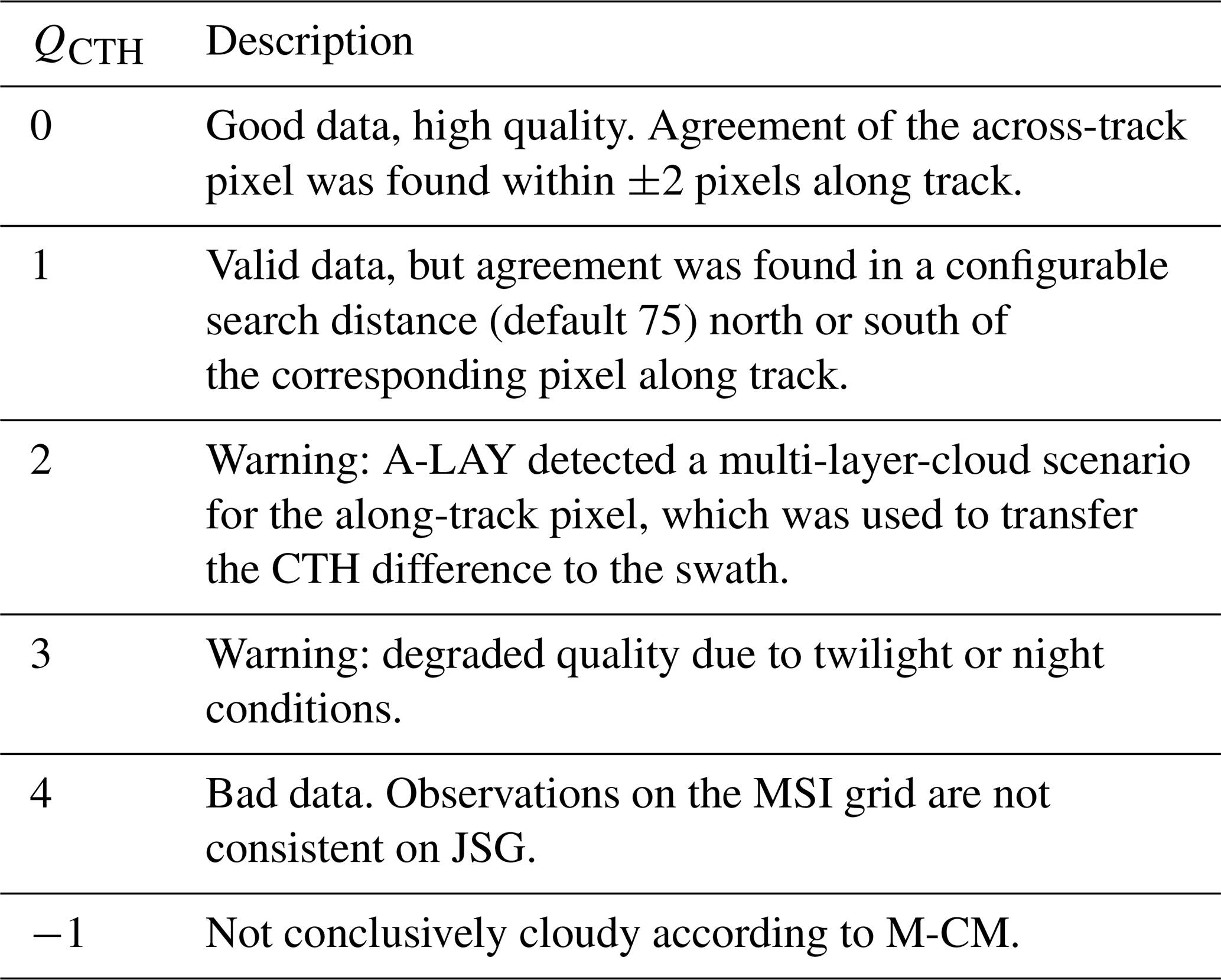
At first, the MSI products (M-CM, M-COP and the MSI L1c data) are mapped on JSG for the entire scene and in an extra step along the track, from which the synergistic ATLID–MSI CTH difference along track is calculated (ATLID minus MSI). The main task is the transfer of the CTH difference to the swath. Therefore, each across-track pixel is compared to the along-track pixels considering the five criteria listed below. In the case of agreement, the CTH difference is transferred. If not, the search for agreement is continued, alternating between north and south along the track. At the end, the quality status of the product is determined (see Table 3).
Table 3The quality status of the cloud top height product (QCTH) is provided for each JSG pixel along and across track on a scale from 0 (highest quality) to 4 (bad quality).
Five criteria are used to relate an across-track pixel to an along-track pixel:
-
agreement in cloud type (International Satellite Cloud Climatology Project (ISCCP) plus multi-layer class)
-
agreement in cloud phase (water, ice, supercooled mixed phase and multi-layer cloud)
-
agreement in surface type (water, land, desert, vegetation, snow, sea ice and sunglint)
-
satisfaction of the criterion in the brightness temperature (10.8 µm) difference threshold (Eq. 1)
-
satisfaction of the criterion in the reflectivity (0.67 µm) difference threshold (Eq. 2).
The cloud phase and surface type are provided in the M-CM product. The AM-CTH algorithm transfers them to JSG resolution under the condition that all contributing MSI pixels must have the same cloud phase or surface type.
In order to transfer the CTH difference detected along track to the entire MSI swath, the cloud type of each JSG pixel has to be determined. The nine cloud classes (cumulus, altocumulus, cirrus, stratocumulus, altostratus, cirrostratus, stratus, nimbostratus, deep convection) defined by the ISCCP (Rossow and Schiffer, 1999) are used to categorize the cloud type of each JSG pixel. ISCCP categorizes the cloud classes by means of the cloud top pressure and the COT. From the MSI pixels contributing to 1 JSG pixel, the lowest cloud top pressure and the corresponding COT are used as input for classifying the JSG pixel. Both quantities are provided in the M-COP product (Table 1). Additionally, a 10th cloud class is defined as the multi-layer class. For the identification of multi-layer-cloud scenarios on the MSI swath, we adapt a method developed by Pavolonis and Heidinger (2004), which was used in M-CLD as well (Hünerbein et al., 2023b). The method makes use of the visible reflectance (at 0.67 µm) and the MSI brightness temperatures at 10.8 and 12.0 µm (T10.8 and T12.0). Pavolonis and Heidinger (2004) simulated the brightness temperature difference (T10.8−T12.0) as a function of the reflectance in order to set a threshold for the multi-layer-cloud detection. The combined ATLID and MSI observations along the satellite track will create a unique dataset to derive this threshold from observations. Along the ATLID track, the vertical information of ATLID easily reveals multi-layer-cloud scenarios (for a semi-transparent upper cloud layer), which are flagged in the simplified uppermost cloud classification of the A-CTH product. There, multi-layer clouds are defined when a configurable number of pixels between two detected cloud layers is cloud-free (default 5 pixels, corresponding to 500 m).
Besides the agreement in cloud type, cloud phase and surface type, two homogeneity criteria are used to determine whether the measured swath pixel can be related to a track pixel. The first criterion is based on a threshold (ΔTth, 10.8) for the difference in the brightness temperature at 10.8 µm (T10.8) between the swath (s) and track pixels (t):
The second criterion uses a threshold (Δρth, 0.67) for the difference in the MSI reflectance ρ0.67 at 0.67 µm between the swath (s) and track (t) pixels:
The thresholds are configurable. The default values are K and based on tests with the simulated EarthCARE test scenes (see Sect. 4). The thresholds can be adapted once real EarthCARE data are available.
In daytime conditions, all five criteria are used to relate a swath pixel to a track pixel. Without sunlight, there is no measurement of the reflectance at 0.67 µm, and the M-COP algorithm cannot determine the COT and thus the cloud type. At nighttime, only three criteria (brightness temperature difference at 10.8 µm and agreement in cloud phase and surface type) are used. The quality status is set accordingly (see Table 3).
The search for agreement is illustrated in Fig. 2b. It starts at the closest along-track pixel and continues by searching 1 pixel before (e.g., to the north) and 1 pixel after (e.g., to the south) from the closest pixel along track. This alternating search is continued until an agreement is found or the configurable maximum search distance is reached (default 75 JSG pixels (approximately 75 km) in each direction along track). If a measurement at the swath agrees with an along-track measurement for all criteria, then the observed CTH difference from the track is assigned to the swath pixel. Otherwise, no CTH difference is assigned to the pixel.
3.2 ATLID–MSI Aerosol Column Descriptor (AM-ACD) algorithm
The structure of the ATLID–MSI Aerosol Column Descriptor (AM-ACD) algorithm is illustrated in Fig. 4. The algorithm is applied to all JSG pixels with a cloud fraction of 0 %. The AM-ACD product contains information on the columnar aerosol optical properties. It provides the spectral aerosol optical thickness (AOT; 355 and 670 nm over land and 355, 670 and 865 nm over the ocean), the respective Ångström exponents and their uncertainties (see Table 2).
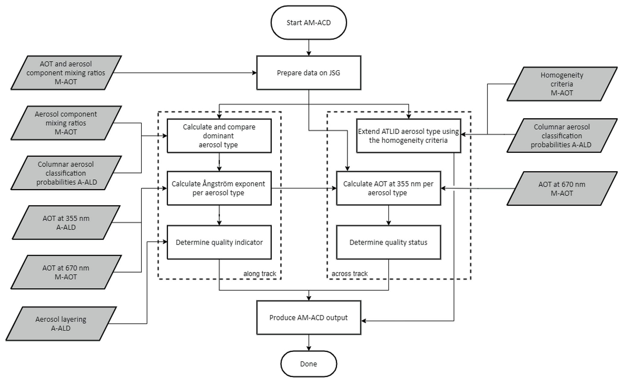
Figure 4Flowchart of the ATLID–MSI Aerosol Column Descriptor (AM-ACD) algorithm. The algorithm is applied to all cloud-free JSG pixels, and it is run after the AM-CTH algorithm.
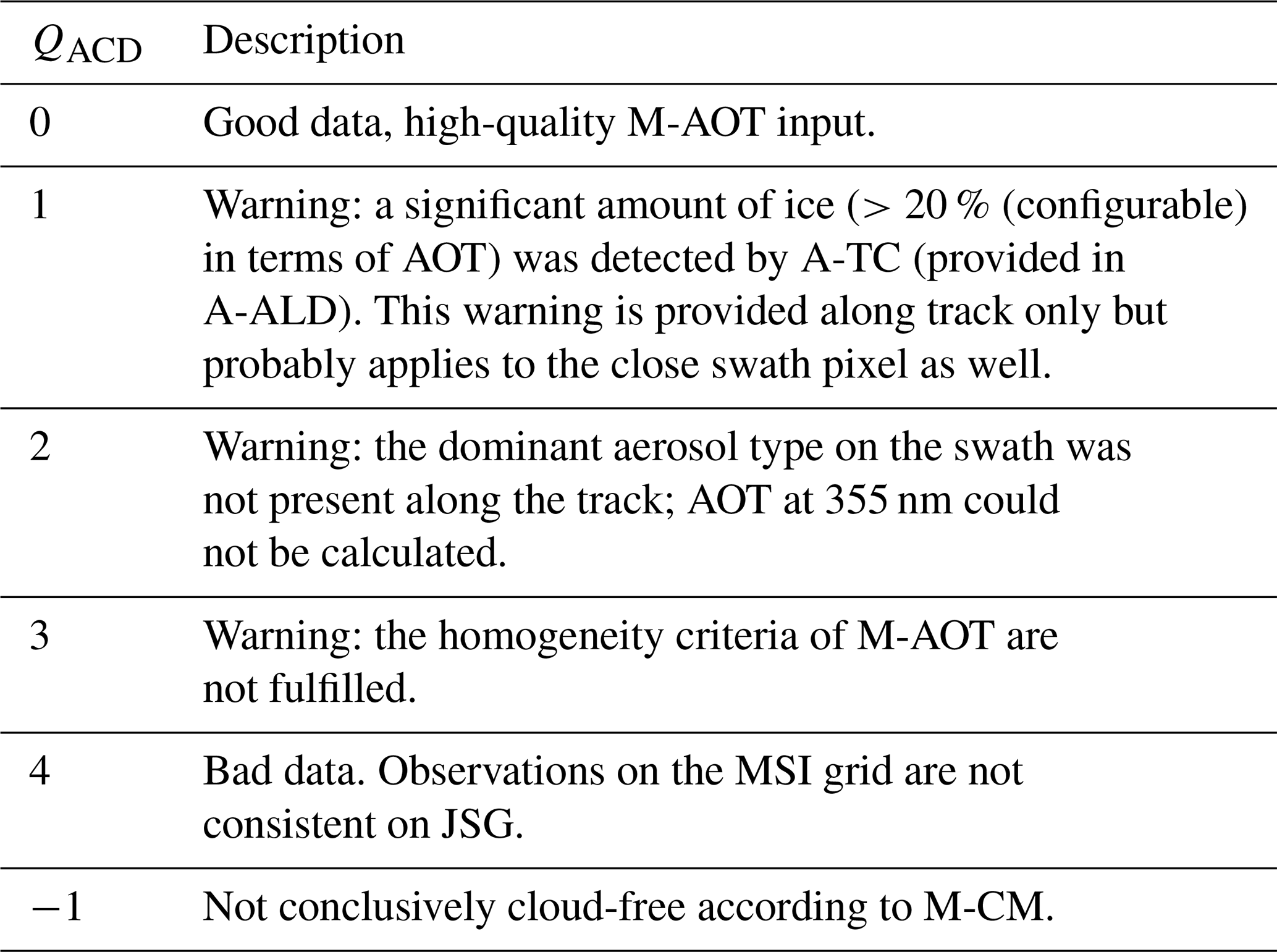
In the first step, ATLID- and MSI-collocated aerosol-type information along track are compared (Sect. 3.2.1), and the Ångström exponent (355/670 nm) is calculated. The ATLID AOT at 355 nm is spread over the swath in the case that the dominant aerosol type agrees between the swath and track (Sect. 3.2.2). By investigating the horizontal homogeneity in the MSI AOT at 670 nm (identification of aerosol plumes), the ATLID aerosol typing can be spread over the entire swath or parts of it (Sect. 3.2.3). The product contains a quality indicator which considers information on the aerosol layering provided by A-ALD, and at the end, an overall quality status of the product is determined (see Table 4).
Table 4The quality status of the aerosol columnar descriptor (QACD) is provided for each JSG pixel along and across track on a scale from 0 (highest quality) to 4 (bad quality).
3.2.1 Comparison of the dominant aerosol type
In Sect. 2.2 the active and passive aerosol typing approaches are introduced. The ATLID aerosol typing is based on the measurements of the linear depolarization ratio and the lidar ratio. Six aerosol types (dust, marine aerosol, continental pollution, smoke, dusty smoke, dusty aerosol mix) and ice are distinguished in the A-TC product (Irbah et al., 2023). The ice is considered to indicate the presence of optically thin ice-containing layers (e.g., diamond dust, subvisible cirrus) that have not been identified as clouds and thus occur in the aerosol products (Irbah et al., 2023; Wandinger et al., 2023b). If the ice aerosol type amounts to a significant contribution (>20 % in terms of AOT, configurable) of the column-integrated aerosol classification, a cirrus cloud that was not detected by the A-CTH algorithm is included in the profile. The profile is therefore not cloud-free, and a warning is issued (see quality status in Table 4). In the following, only the six aerosol types (excluding the ice) are considered for comparison between ATLID and MSI aerosol classifications. The aerosol types are provided as a vertical profile in the A-TC product and are used by the A-ALD algorithm to calculate the column-integrated aerosol classification probabilities for a better comparison with MSI.
The MSI aerosol typing is based on an a priori aerosol climatology over land taken from Kinne et al. (2013) and on a best-fitting component mixture of the MSI measurements over the ocean (Docter et al., 2023). The M-AOT aerosol classification uses 25 mixtures of the four aerosol components defined by HETEAC (see Table 2 in Docter et al., 2023). The four HETEAC aerosol components include two fine modes (weakly absorbing and strongly absorbing) and two coarse modes (spherical and non-spherical), as described in Wandinger et al. (2023a).
The dominant aerosol type is defined by the highest columnar aerosol classification probability (A-ALD product). In Table 5, the six A-TC aerosol types are expressed in terms of the four HETEAC aerosol components which are used in M-AOT. The first four A-TC types (dust, marine aerosol, continental pollution, smoke) are clearly dominated by one of the four HETEAC components even if other aerosol components contribute to these types. The A-TC aerosol types dusty smoke and dusty aerosol mix are a mixture of two or three HETEAC aerosol components. Both mixtures are found for an AOT contribution of coarse-mode non-spherical (CMNS) aerosol between 25 % and 50 %. The more-absorbing dusty smoke requires more than 20 % of fine-mode strongly absorbing (FMSA) aerosol, whereas the less-absorbing dusty aerosol mix should have a contribution of less than 20 % of fine-mode strongly absorbing aerosol.
Table 5The representation of the six aerosol types from the ATLID target classification (A-TC; Irbah et al., 2023) in terms of AOT contributions of the four basic aerosol components defined in HETEAC (Wandinger et al., 2023a) which are used in M-AOT: fine-mode weakly absorbing, FMWA; fine-mode strongly absorbing, FMSA; coarse-mode spherical, CMS; and coarse-mode non-spherical, CMNS. The optical properties (the particle linear depolarization ratio and the lidar ratio at 355 nm) and uncertainty ranges are provided for each A-TC aerosol type.
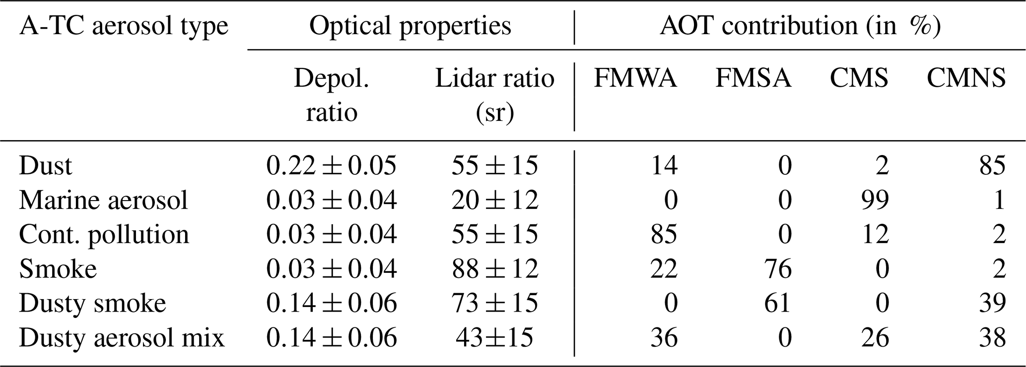
Along the ATLID track, a direct comparison of the six A-TC aerosol types and the four HETEAC components, whose mixing is provided by M-AOT, is achieved. If A-TC is dominated by a mixture (dusty smoke or dusty aerosol mix), the derived thresholds above are applied to the comparison with the M-AOT aerosol classification. In the case of agreement, the dominant aerosol-type flag is set to 1; otherwise it is 0.
3.2.2 Extrapolation of the AOT at 355 nm from the track to the swath
The idea of the AM-ACD algorithm is to extrapolate the AOT at 355 nm, as measured with ATLID, to the MSI swath in order to increase the aerosol information over the entire swath. Therefore, it is important to capture the spatial extent of an aerosol plume across track and combine it with the measurements along track. ATLID observes the AOT at 355 nm and the MSI at 670 and 865 nm over the ocean and 670 nm over land. The Ångström exponent describes the spectral AOT behavior. It is an aerosol-type characteristic parameter which mainly contains information on the mean size of the particles (e.g., Toledano et al., 2007).
If the dominant aerosol type agrees (see Sect. 3.2.1), the AM-ACD algorithm calculates the Ångström exponent (355/670 nm) along track. In every EarthCARE frame ( orbit), the mean Ångström exponent is calculated per dominant aerosol type (if it is present within the frame). From the MSI aerosol classification the dominant aerosol type (in terms of the six A-TC types) is derived for each JSG pixel across track. In the case that the same dominant aerosol type is detected along track as well, the respective Ångström exponent is used to calculate the AOT at 355 nm from the MSI-derived AOT at 670 nm. An aerosol plume consisting of a dominant aerosol type, which is just present on the MSI swath but not on the ATLID track, cannot be handled by the AM-ACD algorithm as the information about the relationship between the two wavelengths is missing.
Alternatively, HETEAC could be used to calculate the Ångström exponent based on the aerosol component mixing ratios (from M-AOT) or the columnar aerosol classification probabilities (from A-TC, A-ALD). However, we decided to implement the described observation-driven approach in AM-ACD.
3.2.3 Extension of the ATLID aerosol classification to the MSI swath
The M-AOT product provides a homogeneity flag (Table 2) which indicates whether the optical properties of the surrounding pixels are counted as homogeneous. This flag is used to transfer the dominant aerosol type derived from ATLID observations along track to the MSI swath. As long as the homogeneity criterion is fulfilled, the same dominant aerosol type as derived for the closest along-track pixel could be assumed for the across-track pixel. The additional M-AOT aerosol typing provides the possibility of comparison.
A simple aerosol classification based on the AOT at 670 nm and the Ångström exponent (355/670 nm) would be possible. Passive remote-sensing techniques have applied this method in the past (e.g., Toledano et al., 2007). However, we do not consider the AOT to be an adequate parameter for aerosol typing because it depends on the amount of aerosol (extensive quantity) and not on the aerosol-type characteristics. As an example, a thin dust layer (low AOT, low Ångström exponent) might be misclassified as marine aerosol. Here, we prefer to extend the ATLID aerosol typing to the swath. It is based on the intensive quantities of the particle linear depolarization ratio and lidar ratio. Moreover, the higher depolarization ratio would clearly identify the dust layer and would not lead to a confusion with marine aerosol. We leave it open to the user to construct their own aerosol classification scheme based on the columnar quantities provided (AOT at 355, 670 and over the ocean additionally at 865 nm and the respective Ångström exponents; see Table 2).
The synergistic AM-COL processor partly uses L1 data from instruments but mainly combines ATLID and MSI L2a products to generate a L2b columnar product. This fact prevents us from using real-world data for its validation. As presented in Sect. 2.1, MODIS-retrieved CTHs are validated against space-lidar-derived CTHs. The synergistic AM-COL processor already combines active and passive remote sensing. Thus, in the present state it can only be validated against simulated test scenes available for the EarthCARE processing chain. Specific test scenes were created with the EarthCARE End-to-End Simulator to test the full chain of EarthCARE processors (Donovan et al., 2023b). All scenes are based on the Global Environmental Multiscale (GEM) model output (Qu et al., 2023b). The aerosol fields are taken from the Copernicus Atmosphere Monitoring Service (CAMS) model. In the following, we present results obtained with the AM-COL processor for the so-called Halifax, Hawaii and Halifax aerosol scenes. A detailed description is presented in Donovan et al. (2023b), in particular in Sect. 3.1, 3.3 and 3.4. Furthermore, we refer to the plots of the ATLID Mie co-polar signal and the CTH in Wandinger et al. (2023b), where the Halifax scene is shown in Fig. 6 and the Halifax aerosol scene in Fig. 9.
4.1 AM-CTH validation
Firstly, the output of the AM-CTH algorithm is presented (Sect. 4.1.1). Then, the output is validated against the GEM model truth (Sect. 4.1.2) with an in-depth discussion on cloud class and multi-layer clouds (Sect. 4.1.3).
4.1.1 AM-CTH output for the Halifax scene
The validation of the AM-CTH product is shown for the Halifax scene. In the first step, we compute the CTH difference (ATLID–MSI) for all cloudy JSG pixels along the ATLID track. In Fig. 5, the CTHs of A-CTH and M-COP are shown together with the CTH difference (AM-CTH) for the Halifax scene along the ATLID track. The CTH difference is small for the scattered clouds in the south (<32∘ N) and for the optically thick cirrus cloud at 36–39∘ N. However, the multi-layer-cloud scenario in the center (39–47∘ N) leads to large differences. MSI is sensitive to the optically thick liquid-containing clouds at a height of 5–7 km, and ATLID detects the thin cirrus cloud at a height of 11 km as CTH. Further north (>50∘ N), nighttime conditions limit the ability of MSI to detect the CTH and lead to a larger scattering. Nevertheless, the agreement is mostly within 2 km, except for the high clouds north of 65∘ N.
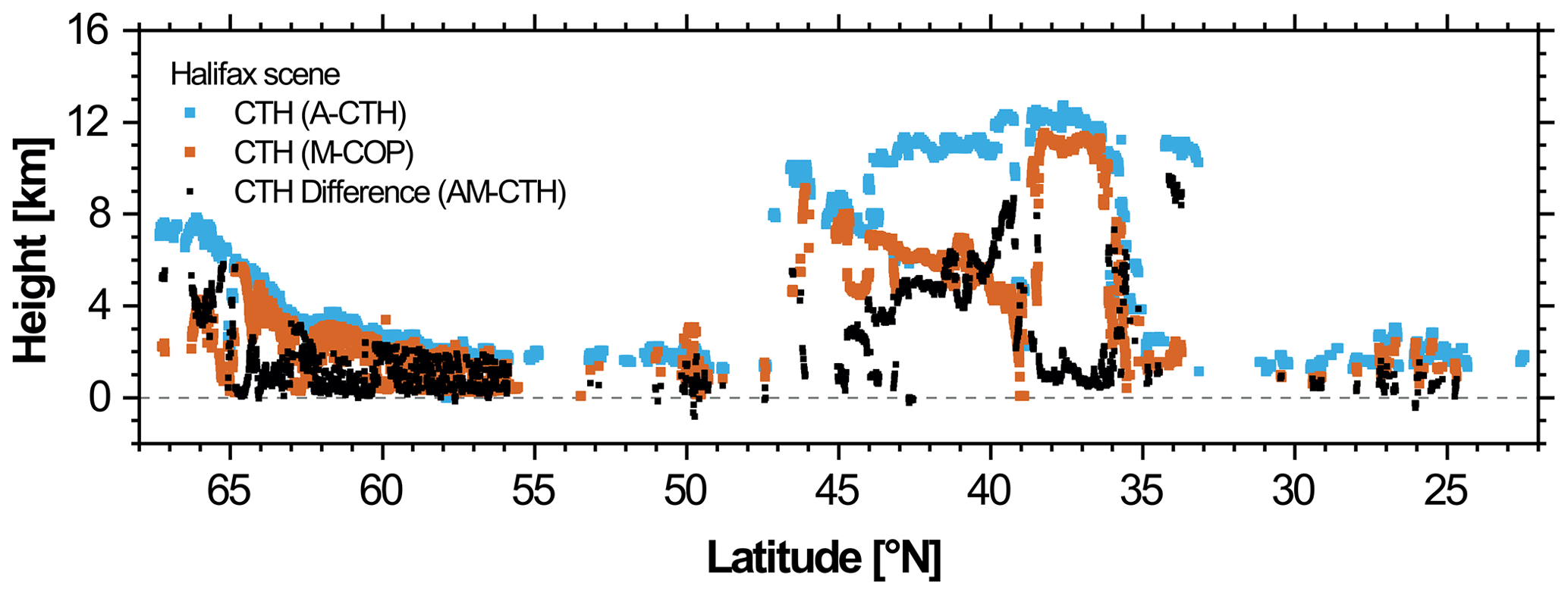
Figure 5CTH along the ATLID track derived by A-CTH (blue dots) and M-COP (orange dots). AM-CTH calculates the difference (black dots) to transfer it to the MSI swath. The results are shown for the Halifax scene. More details concerning the ATLID CTH are shown in Fig. 6 of Wandinger et al. (2023b).
Figure 6 presents the five quantities needed to transfer the CTH difference from the track to the swath. The reflectivity (Fig. 6d) cannot be measured at nighttime, and the cloud type (Fig. 6a) is not retrieved for nighttime or twilight conditions (>50∘ N). Then, only the remaining three criteria can be applied. During nighttime, the cloud-phase retrieval (Fig. 6b) alternates between ice and supercooled mixed-phase clouds. Only if all contributing MSI pixels show the same cloud phase is a cloud-phase value assigned to the JSG pixel. Otherwise no CTH difference is transferred for the JSG pixel. It results in white spots in Fig. 7b and a decreased quality status. The brightness temperature at 10.8 µm (Fig. 6c) provides information about the scene during the day and night and is therefore a valuable input parameter. The surface (Fig. 6e) does not depend on the cloud properties. The criterion of the same surface is rather conservative in order to ensure that only similar MSI pixels are used for the track-to-swath method.
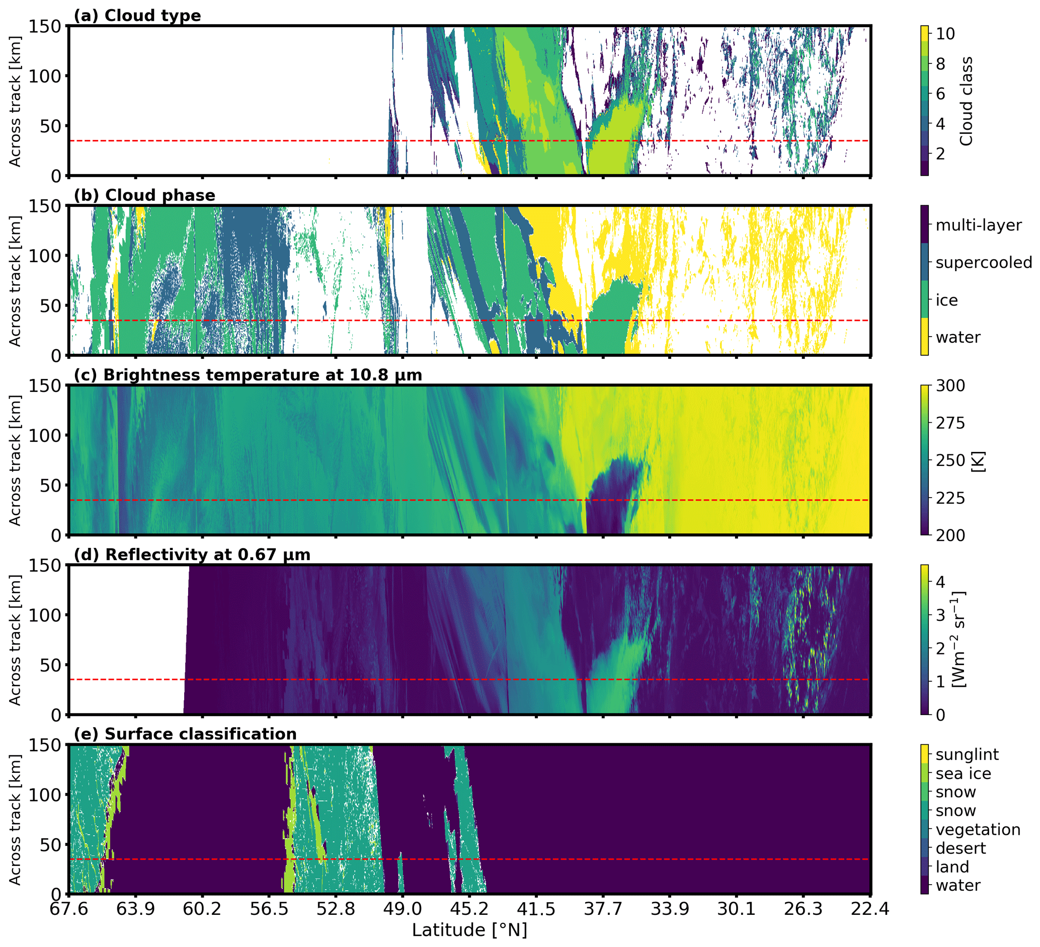
Figure 6MSI input for the Halifax scene on JSG: (a) cloud type defined by the nine ISCCP classes (1–9) and the multi-layer class (10), (b) cloud phase, (c) brightness temperature at 10.8 µm, (d) reflectivity at 0.67 µm, and (e) surface type (detailed description in Hünerbein et al., 2023b). The ATLID track is marked with a dashed red line. Note that the aspect ratio does not reflect the real situation, which is approximately 5000 km along track and 150 km across track.
Figure 7 shows the MSI-derived CTH (on JSG), the synergistic ATLID–MSI CTH difference and the AM-CTH quality status. North of 50∘ N, no sunlight is present (nighttime observations), leading to limitations in the M-COP retrieval, which are accounted for in the quality status (Fig. 7c). The quality status is 3 (or worse). Here, only three of the five criteria for the track-to-swath transfer could be applied. Cloud-free parts are shown in black for the AM-CTH products. The CTH difference is color-plotted over the cloudy parts shown in white. AM-CTH can provide a CTH for half of the cloudy JSG pixels (51 %) defined by MSI. There are several reasons why a CTH difference cannot be transferred from the track to the swath: (1) the field of high cirrus clouds in the center cannot be transferred for the entire swath. For the across-track pixels >60, no along-track pixels agreeing in all five criteria can be found within ±75 pixels in each direction to transfer the CTH difference. Even a larger search distance of 150 pixels would only increase the number of agreeing across-track pixels slightly (58 %). (2) During the nighttime observations (>50∘ N), the limited information from M-COP and a quickly changing cloud phase (one of the three nighttime criteria) make the transfer of the synergistic CTH difference difficult. (3) A changing surface below the scene further limits the ability of the possible along-track pixels to transfer the CTH difference (see Fig. 6e).
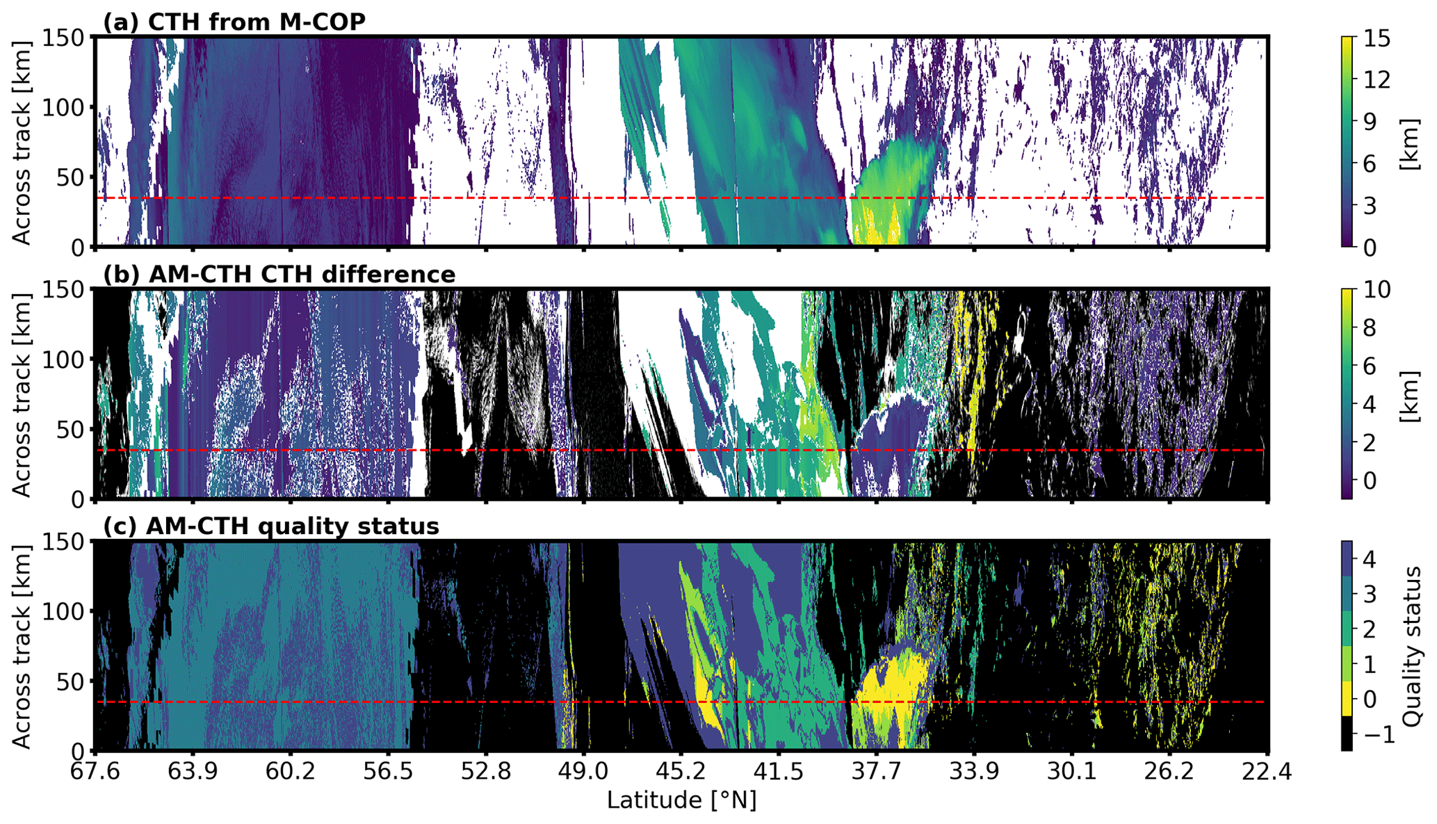
Figure 7(a) CTH for the Halifax scene as detected with MSI (M-COP algorithm, now on JSG) and (b) the synergistic ATLID–MSI CTH difference (AM-CTH product). The black areas are cloud-free. In the white areas M-CM detected a cloud which was not transferred by AM-CTH. (c) The quality status of the AM-CTH product ranging from 0 (high quality) to 4 (bad quality). A quality status of −1 is given to (cloud-free) pixels for which AM-CTH was not applied. The ATLID track is marked with a dashed red line.
The large CTH differences in the center of the scene originate from the thin cirrus above the liquid-containing clouds, as already seen in the CTH difference along track (Fig. 5). The large CTH difference around 34∘ N is probably a misinterpretation of the AM-CTH algorithm due to a thin cirrus which is present along track above the low clouds. The CTH difference is small (<2 km) in the case of the mixed-phase clouds north of 55∘ N, the optically thick cirrus in the center and the shallow marine cumulus clouds in the south of the scene. The algorithm performance is compared against the model truth in the following subsection. Then, different cloud types are studied in more detail in Sect. 4.1.3.
4.1.2 CTH validation against the model truth
The results of the AM-CTH algorithm are validated against the GEM model truth (Qu et al., 2023b; Donovan et al., 2023b). In the model, the extinction coefficients for cloud water and cloud ice are provided. The central question is as follows: how can CTH be defined based on the true cloud extinction fields? Here, we follow two distinct approaches: an extinction threshold and a cloud optical thickness (COT) threshold.
The ATLID-based approach as followed in the A-CTH validation uses an extinction threshold. The CTH is defined when the cloud extinction reaches (coming from above) a certain threshold value for the first time. In the A-CTH validation an extinction threshold of 20 Mm−1 provides reasonable agreement between the derived CTH and the model truth (Wandinger et al., 2023b). It provides an indication of the ability of the A-CTH algorithm to detect CTHs. This method defines the cloud as a geometrical feature and is sensitive to optically thin and thick clouds.
The MSI-based approach, as followed in the M-CLD validation (Hünerbein et al., 2023a, b), uses a COT threshold approach. Coming from above, the extinction coefficient is integrated until a certain threshold COT is reached. Here, a COT threshold of 0.25 is used following the investigations of Stengel et al. (2015). They applied this threshold to CALIPSO-derived CTHs to get a better agreement with CTHs derived from passive imagers considering the different capabilities in CTH detection. This method defines the cloud as a radiative feature and is rather sensitive to optically thicker clouds.
Both methods to derive the true CTH from the GEM model truth are compared in Fig. 8. The results are shown for the 364×103 cloudy JSG pixels detected by the MSI cloud mask in the Halifax scene. Here, we do not want to validate the MSI cloud mask (already done in Hünerbein et al., 2023b) but the CTH. Therefore, we take the true CTH only for the 364×103 pixels defined as cloudy by M-CM. It will lead to more cloudy pixels if we define the clouds from the true extinction fields. From the scatterplot, it can clearly be seen that the CTH defined by an extinction threshold of 20 Mm−1 is always equal or higher compared to the COT threshold of 0.25. However, in 65 % of the cloudy pixels, the CTH agrees within ±300 m. The high clouds (>10 km height) in particular are optically thin and reach the COT threshold of 0.25 at a lower altitude. For the validation against the model truth, we follow both CTH definitions, as the best solution depends on the research interests of the users.
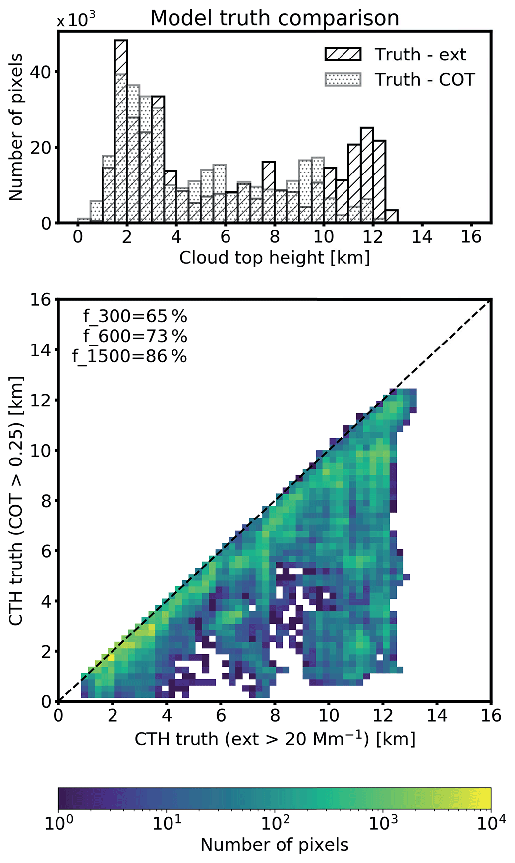
Figure 8Comparison of the true CTH from GEM model output for the Halifax scene derived via an extinction threshold of 20 Mm−1 (hatched) and a COT threshold of 0.25 (dotted) for all 364×103 JSG pixels with a cloud fraction of 100 %. The indicator fi displays the percentage of data points within ±i m from the 1:1 line. The scatterplot shows that the CTH based on the extinction threshold is always higher or equal compared to the COT threshold.
The validation with the extinction threshold is shown in Fig. 9 for the MSI-only and the ATLID–MSI retrieval as a histogram and scatterplot. M-COP provides a CTH for 350×103 JSG pixels (96 %) of the 364×103 pixels detected as cloudy by the MSI cloud mask due to further quality checks in the M-COP algorithm. The AM-CTH algorithm could not assign a CTH difference for every cloud found by M-CM because several homogeneity criteria (see Sect. 3.1) have to be fulfilled to confidently translate a CTH difference from the track to the swath. AM-CTH can provide a CTH for only half of the CTHs (177×103, 51 %) provided in M-COP. In the case of AM-CTH, 63 % of the detected CTHs are within ±600 m from the 1:1 line, and 40 % are within ±300 m, which is defined in the mission requirements. Some cirrus clouds on the swath are not detected, and the CTH is thus underestimated. In some other cases, AM-CTH transfers a high (cirrus) CTH to the swath, although there are only low clouds present. Both issues occur on the swath, where only the MSI information is present. In the majority of the cases, AM-CTH captures the (geometric) CTH. The standalone MSI retrieval tends to underestimate the (geometric) CTH, especially for the high clouds and some of the low clouds (see further separate discussion about cloud types in Sect. 4.1.3); however, 22 % of the detected CTHs are within ±600 m from the 1:1 line.
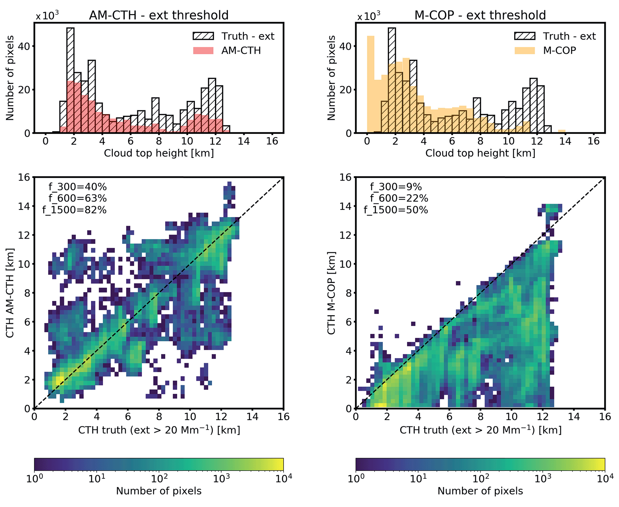
Figure 9CTH validation against the GEM model truth for the Halifax scene. The true CTH is determined by the ATLID-based definition with a cloud extinction threshold of 20 Mm−1 for all cloudy pixels detected by the MSI cloud mask. The histograms and scatterplots are shown for the ATLID–MSI synergy product (AM-CTH, left) and the MSI-only product (M-COP, right). The indicator fi displays the percentage of data points within ±i m from the 1:1 line.
The situation changes when considering the COT-based threshold for defining the true CTH (Fig. 10). Here, M-COP shows a much better agreement because the threshold is less sensitive to the thin cirrus clouds and represents the radiative CTH (Stengel et al., 2015). Now, 53 % of the M-COP CTHs fall within ±600 m of the 1:1 line. AM-CTH overestimates the (radiative) CTH, showing a positive bias to the 1:1 line (37 % within ±600 m). The cirrus clouds between 9 and 13 km height are in particular detected by AM-CTH below a COT of 0.25.
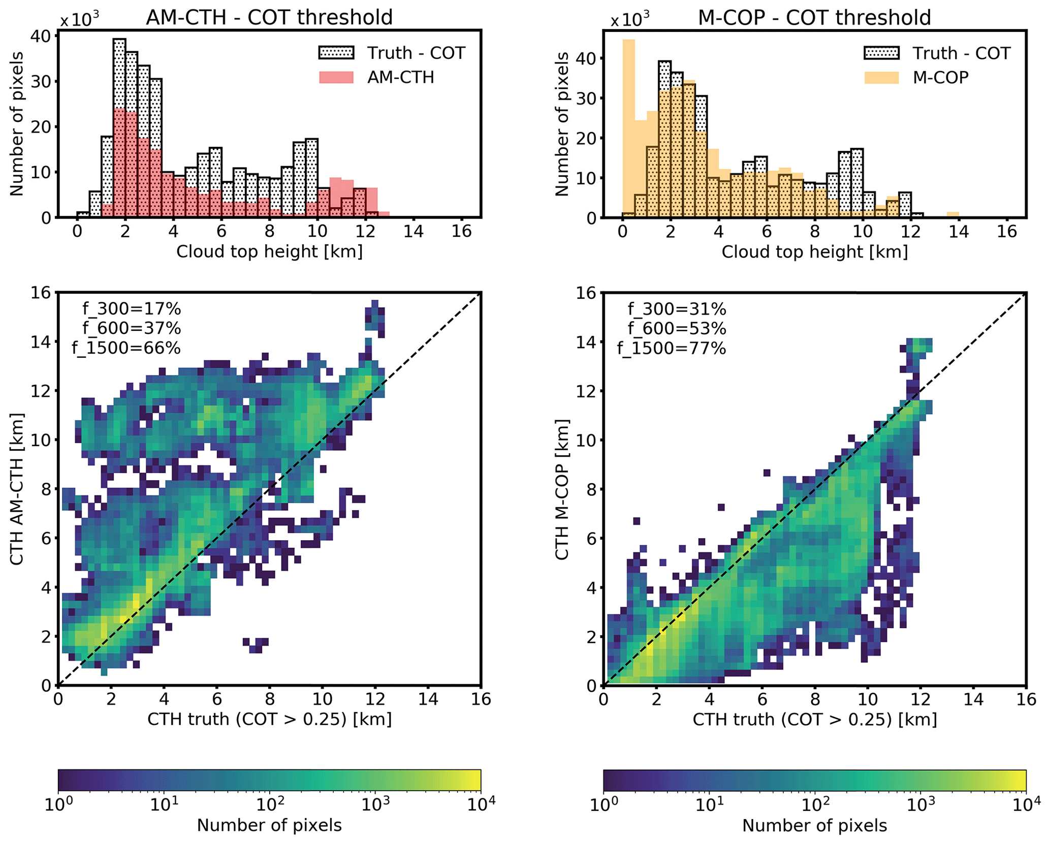
Figure 10The same as Fig. 9, but here the true CTH is determined by the MSI-based definition with a COT threshold of 0.25.
The number of data points within an interval of ±i m around the 1:1 line (fi in Figs. 9 and 10) shows a similar behavior for AM-CTH to the extinction-based model truth (40 %, 63 % and 82 % for 300, 600 and 1500 m) and for M-COP to the COT-based model truth (31 %, 53 % and 77 % for 300, 600 and 1500 m). This behavior underlines the finding that the extinction-based geometric CTH is detected by AM-CTH and the COT-based radiative CTH is detected by M-COP. In the following, we follow the extinction-threshold-defined CTH. A separation per ISCCP cloud type is provided in Sect. 4.1.3, with special focus on the multi-layer-cloud scenarios.
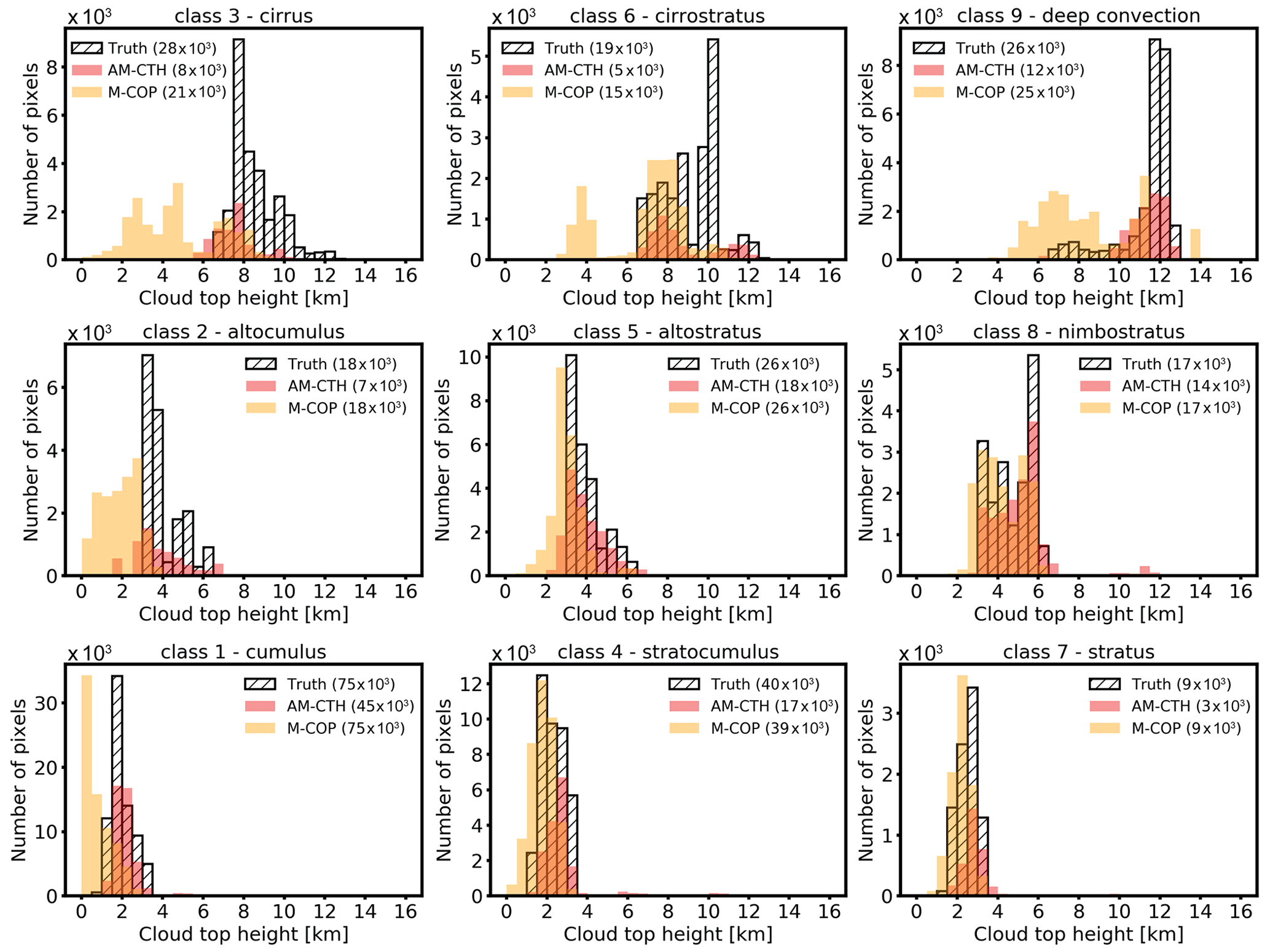
Figure 11Histograms of the CTH validation against the GEM model truth (hatched) for the nine ISCCP cloud classes. The cloud class is defined by the GEM model truth using an extinction threshold of 20 Mm−1 for the CTH detection. The multi-layer clouds are not included. The outputs of M-COP (orange) and AM-CTH (red) for the same pixel are presented for the Halifax scene. The total number of pixels is provided for each cloud class in brackets.
4.1.3 AM-CTH algorithm performance for different cloud classes
The performance of the AM-CTH algorithm is tested for the nine ISCCP cloud classes (Rossow and Schiffer, 1999) and the multi-layer class. The detection of the latter is mainly based on the work by Pavolonis and Heidinger (2004). However, the brightness temperature difference between 10.8 and 12.0 µm is not simulated sensitively enough in the EarthCARE test scenes to clearly detect multi-layer clouds with MSI. Figure 11 presents the histograms of the CTH detected by M-COP (orange), the synergistic CTH by AM-CTH (red) and the true CTH (hatched) from the GEM model based on an extinction threshold of 20 Mm−1 for all clouds detected by the MSI cloud mask in the Halifax scene. In Fig. 11, the cloud class for each JSG pixel is determined by the GEM model output (CTH determined with an extinction threshold of 20 Mm−1 and COT). The corresponding M-COP and AM-CTH results are sorted in the same cloud-class category. The best agreement between M-COP and the model truth is reached for stratus, nimbostratus and stratocumulus clouds which are optically thick. AM-CTH is based on M-COP and thus agrees well with the model truth for these cloud classes. The AM-CTH algorithm improves the (geometric) CTH detection compared to M-COP in two areas: (1) high clouds, which are underestimated by M-COP as they are too thin to be detected with MSI, and (2) cumulus and altocumulus clouds for which the CTH is detected too low by MSI. A closer inspection of the vertical profiles of the extinction in each cloud class showed that the maximum in the extinction, and thus optical depth, is reached much lower than the geometric CTH, especially for the optically thin clouds (left column of Fig. 11) and the high clouds (top row of Fig. 11). In general, MSI underestimates the CTH if we consider the geometric boundaries of the cloud by applying an extinction-based threshold (Figs. 9 and 11). MSI is sensitive to the radiative boundary of the cloud (see COT-based threshold in Fig. 10), which coincides with the geometric boundary in the case of optically thick clouds such as stratus, nimbostratus and stratocumulus clouds.
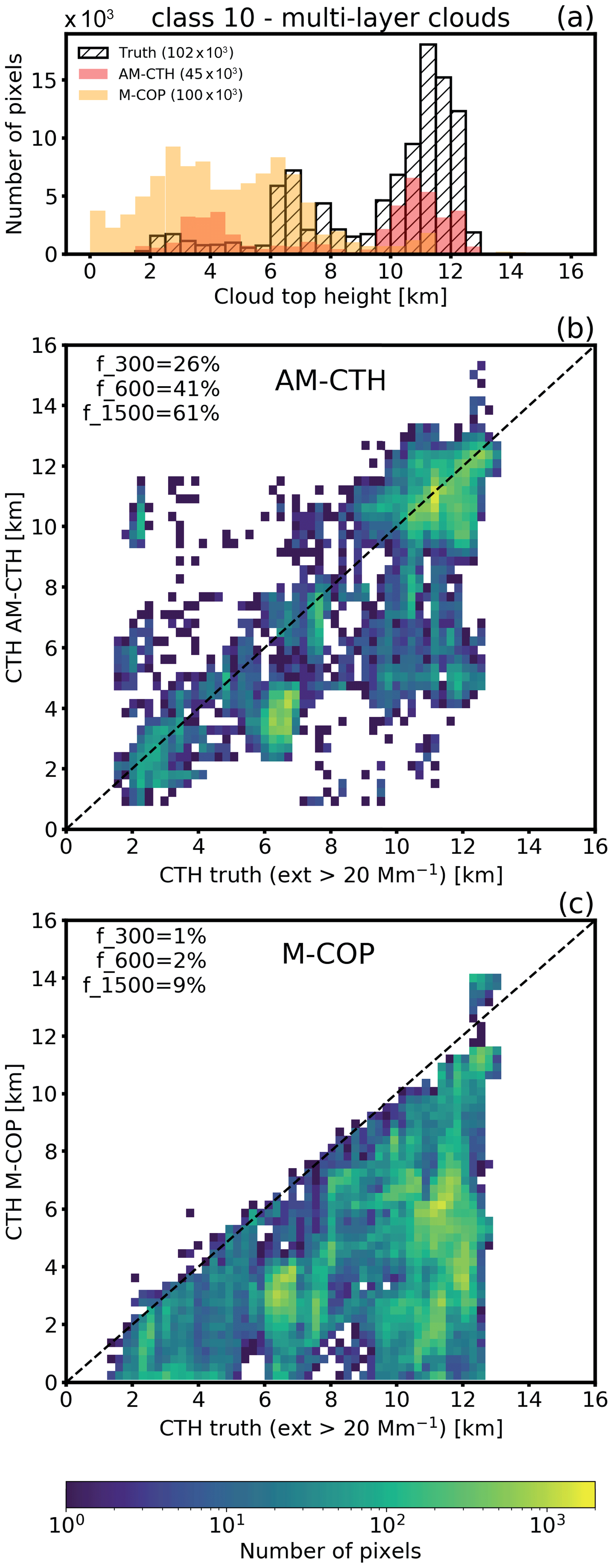
The number of JSG pixels considered in the histogram is provided in the plots. As previously stated (Sect. 4.1.2), AM-CTH is able to transfer a CTH difference for half of the CTHs (51 %) provided in M-COP in the case of the Halifax scene. A special challenge is the multi-layer clouds for which the results are presented in Fig. 12. The definition applied to the GEM model output follows the criteria introduced in the A-CTH algorithm (Wandinger et al., 2023b) stating that at least five height bins corresponding to approximately 500 m of clear air has to be present between two cloud layers to be classified as multi-layered. The multi-layer clouds are not included in the nine ISCCP cloud classes (Fig. 11) but are treated on top as a 10th cloud class as implemented in the AM-CTH algorithm. The multi-layer clouds are the most frequent cloud class in the Halifax scene with 102×103 JSG pixels (28 % of all cloudy pixels defined by M-CM). Figure 12 clearly shows that the CTH of the high clouds dominates the multi-layer CTH. Here, AM-CTH significantly improves the (geometric) CTH detection compared to the standalone MSI algorithm (M-COP). A total of 41 % instead of 2 % of the CTHs are detected within ±600 m from the 1:1 line. The second peak in the true CTH between a height of 6 and 8 km is underestimated by both M-COP and AM-CTH. These clouds are further away from the track, and the CTH derived by the AM-CTH algorithm is based on the MSI measurements. Nevertheless, the ATLID–MSI columnar products improve the CTH detection, especially in the case of multi-layer clouds and single-layer high and optically thin clouds compared to the standalone MSI retrieval. MSI is sensitive to the radiative CTH rather than the geometric CTH (see Fig. 8).
4.2 AM-ACD validation
Firstly, the output of the AM-ACD algorithm for the Halifax aerosol scene is presented (Sect. 4.2.1). Then, the more complex aerosol conditions in the Hawaii scene are analyzed (Sect. 4.2.2). Lastly, the output of both scenes is validated against the CAMS model truth (Sect. 4.2.3).
4.2.1 AM-ACD output for the Halifax aerosol scene
The Halifax aerosol scene is created for the validation of aerosol retrievals and contains only marine aerosol and some ice clouds. The dominant aerosol type for the cloud-free pixels along track is correctly classified by M-AOT and A-ALD as coarse-mode spherical and marine aerosol, respectively. The AOT along track for all wavelengths is shown in Fig. 13. M-AOT provides the AOT at 670 and 865 nm. A-ALD contains the AOT at 355 nm from the integrated extinction coefficient taken from the A-EBD product at medium resolution. The ice cloud at 34∘ N is only partly detected by the MSI cloud mask, and thus the optical thickness of the ice crystals is included in the M-AOT product. At 35∘ N, even the cirrus is too thin to be detected by A-LAY, which classifies the corresponding profiles as cloud-free and starts the aerosol retrievals (A-ALD algorithm). The additional optical thickness of the ice crystals increases the AOT in the A-ALD product and leads to an overestimation compared to the CAMS model truth AOT, which is provided for aerosol only. In the southern part of the scene in particular, the AOT values at 355 nm scatter a lot. The A-ALD AOT in this marine-aerosol-dominated scene is lower compared to the model truth by for the scene <32.5∘ N, which is not influenced by the cirrus cloud. A possible reason for the underestimation of the AOT is the extinction calculation of the A-PRO processor (Donovan et al., 2023a). The high standard deviation is caused by the scattering of the A-ALD AOT values. Nevertheless, the deviation from the model truth is within the accuracy of 0.05 for the AOT, as demanded by the EarthCARE mission requirements (MRD, 2006).
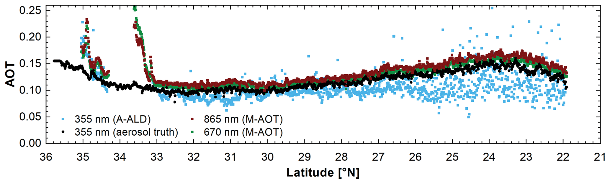
Figure 13AOT along the ATLID track in the Halifax aerosol scene derived by ATLID (355 nm, blue) and MSI (670 nm, green, and 865 nm, brown). The true AOT at 355 nm is shown in black for aerosol only, regardless of the clouds above. The ATLID scene, i.e., the Mie co-polar signal, is shown in Fig. 9 of Wandinger et al. (2023b).
In the next step, the Ångström exponent (355/670 nm) is calculated along track. The Ångström exponent per dominant aerosol type is obtained by averaging the Ångström exponents for all pixels along track for which the dominant aerosol type of both input algorithms (M-AOT and A-ALD) agrees. Only marine (coarse-mode spherical) aerosol is present in the Halifax aerosol scene. An Ångström exponent for the other types is not derived as they are not present along track. The derived Ångström exponent for marine aerosol (coarse-mode spherical) is . HETEAC defines an Ångström exponent of −0.16 for pure coarse-mode spherical aerosol in the respective wavelength range (Wandinger et al., 2023a). The too low extinction coefficient derived from ATLID and the consequently too low AOT at 355 nm are the reasons for the deviation of the Ångström exponent. The scattering in the A-EBD results leads to the high standard deviation. Nevertheless, the derived Ångström exponent is used to calculate the AOT at 355 nm on the swath from the AOT at 670 nm. The results are presented in Fig. 14 together with the quality status of the AM-ACD product.
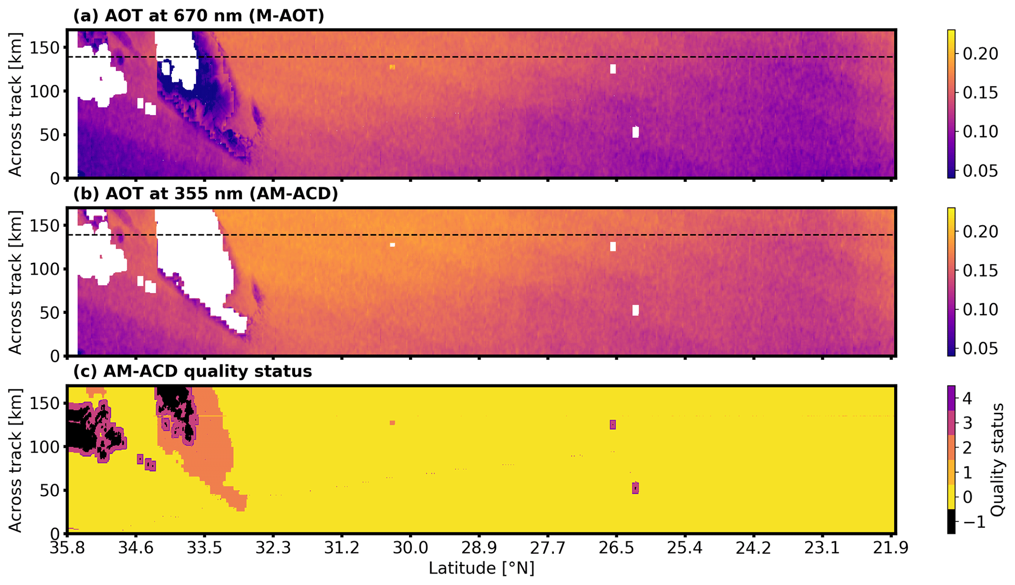
Figure 14AOT at 670 (a) and 355 nm (b) and the AM-ACD quality status (c) for the Halifax aerosol scene. The ATLID track is marked with a dashed black line, except for panel (c) so as to not overlay the quality status of 1, which is only reported along track. For the pixels categorized as cloudy, M-AOT does not derive an AOT (white areas in panel (a)). Still, some ice clouds are present, which leads to an increased AOT (>32.5∘ N). The M-AOT algorithm derives a different aerosol mixture for the cloud-influenced pixels. This mixture does not agree along track, and therefore these pixels are not considered in the transference of the AOT at 355 nm from the track to the swath (larger white area in panel (b)). This behavior is reflected in the quality status of AM-ACD, which ranges from 0 (high quality) to 4 (bad quality); details are provided in Table 4.
4.2.2 AM-ACD output for the Hawaii scene
More aerosol types are present in the Hawaii scene, which will be shown to demonstrate the performance under complex aerosol conditions. The dominant aerosol type shown in Fig. 15a was derived from the M-AOT aerosol mixing ratios as described in Sect. 3.2.1. Most of the scene is dominated by fine-mode aerosol, which is classified as smoke, continental pollution and dusty smoke because of similar optical properties. Only south of 16∘ S does marine aerosol dominate. A wide area in the Northern Hemisphere is affected by sunglint, which leads to an increased uncertainty in the M-AOT product. In these areas, the quality status of AM-ACD is 3, as seen in Fig. 15c. Thus, in the following we focus on the southern hemispheric part of the Hawaii scene. The obtained AOT at 355 nm is presented in Fig. 15b. The comparison with the model truth is provided in the next subsection.
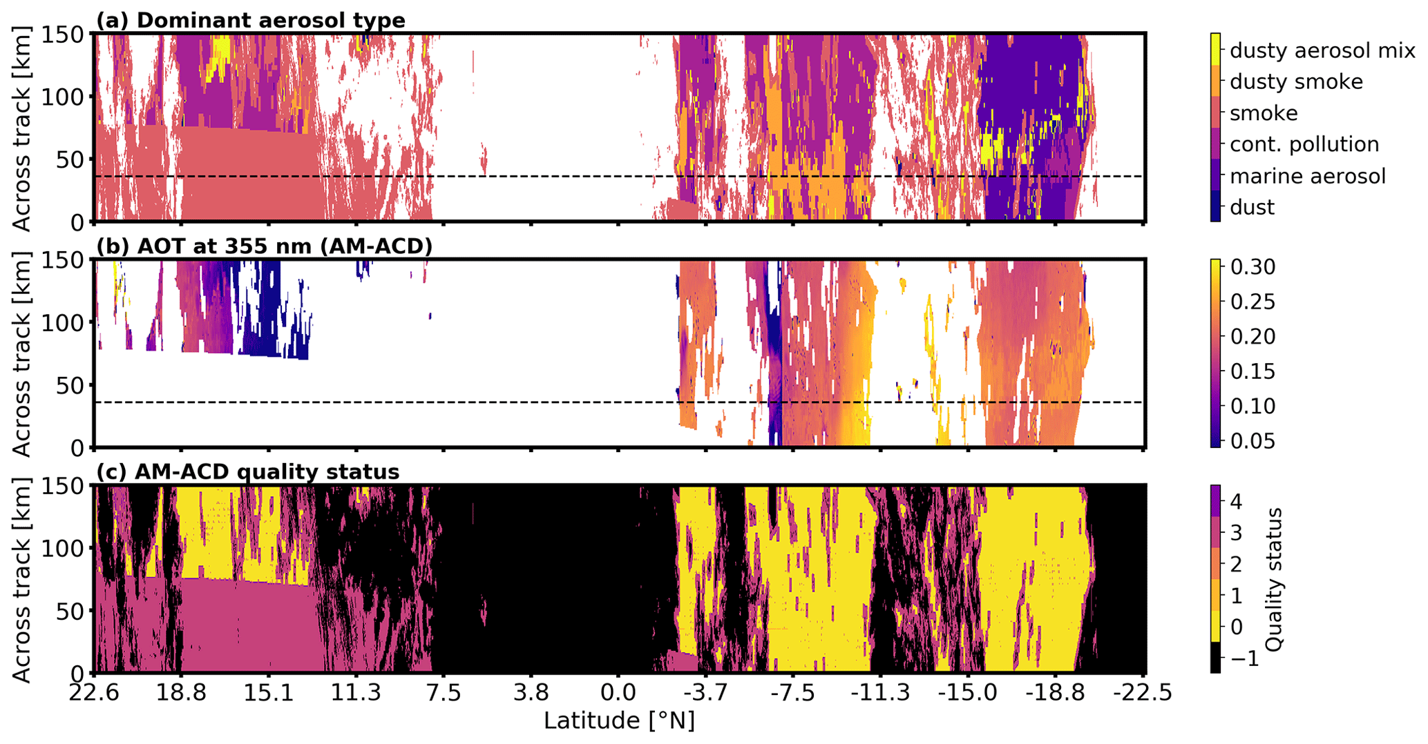
Figure 15The dominant aerosol type (a), AOT at 355 nm (b), and AM-ACD quality status (c) for the Hawaii scene. The quality status ranges from 0 (high quality) to 4 (bad data). A quality status of −1 represents cloudy pixels for which the AM-ACD algorithm is not applied. The dominant aerosol type follows Table 5. The ATLID track is marked with a dashed black line, except for panel (c) so as to not overlay the quality status of 1, which is only reported along the track.
4.2.3 Aerosol product validation against the model truth
The AM-ACD products are validated against the model truth available for the simulated test scenes. Firstly, we discuss the Halifax aerosol scene and then the Hawaii scene.
In the Halifax aerosol scene, the dominant aerosol type agrees for the entire scene, except for the cloud-influenced pixels. The AOTs at 670 and 865 nm are taken from the M-AOT product (now provided on JSG) and are validated in Docter et al. (2023). The validation of the AOT at 355 nm on the MSI swath is presented in Fig. 16. The high AOT values between 0.20 and 0.25, which are not present in the model truth, are caused by an incorrect aerosol–cloud discrimination. The validation is done for latitudes <32.5∘ N which are not influenced by any cloud (Fig. 16b). The majority of the pixels follows the 1:1 line with a small negative offset of . The offset is caused by the negative offset of the AOT at 355 nm from upstream processors, namely the extinction calculations in A-PRO ().
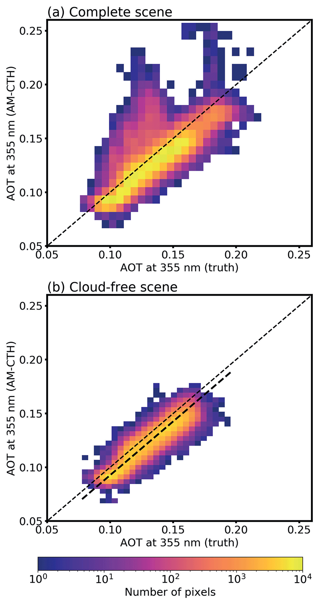
Figure 16The AOT at 355 nm derived with AM-ACD in the Halifax aerosol scene is compared against the model truth. (a) The results for the entire scene are shown. The cirrus clouds lead to an overestimation of the AOT. (b) The scene is shown for a latitude < 32.5∘ N, where no clouds are present (see Fig. 14). Under cloud-free conditions, the AOT is underestimated. The linear fit, shown as a thick dashed line, indicates the mean offset of .
In the case of the Hawaii scene, the agreement is less good. In Fig. 17, we first compare the AOT at 670 nm against the model truth and see that the majority of the pixels follows the 1:1 line. The comparison is restricted to the Southern Hemisphere and an AM-ACD quality status of 0. The overestimation of the AOT at 670 nm (mean offset 0.013±0.026) by the M-AOT algorithm is caused by thin cirrus clouds which are not detected by M-CM. Therefore, these pixels are processed by the aerosol algorithm and lead to an increased AOT. AM-ACD uses the AOT at 670 nm to calculate the AOT at 355 nm on the swath. Therefore, this overestimation continues in the AM-ACD product. Moreover, the overestimation increases for the AOT at 355 nm. A mean offset of 0.054±0.035 (indicated by the dashed line) is found under these complex aerosol conditions. It is slightly above the mission requirements of 0.05.
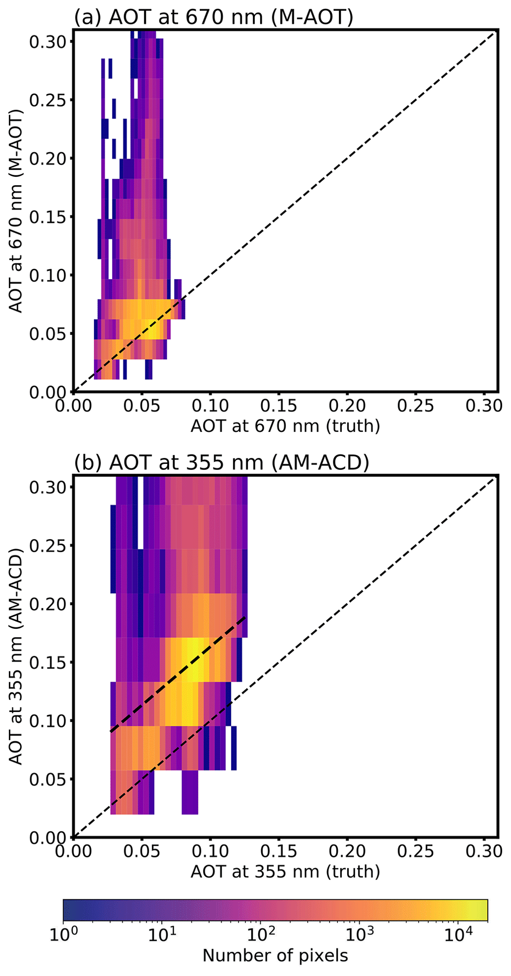
Figure 17The AOT at 670 nm from M-AOT (a) and at 355 nm from AM-ACD (b) in the Hawaii scene is compared against the model truth. Here, the results are shown for the Southern Hemisphere and only for the pixels with an AM-ACD quality status of 0. The thick dashed line indicates the mean offset of 0.054±0.035 found for the AOT at 355 nm.
In summary, the method applied in the AM-ACD algorithm itself leads to a good agreement with the model truth in the case of the simple Halifax aerosol scene. Even for the more complex aerosol situation in the Hawaii scene, the results are only slightly above the mission requirements. The AOT validation at 355 or 670 nm across all simulated test scenes for various processors (e.g., A-EBD, M-AOT and ACM-CAP) is provided in Chap. 3.4 of Mason et al. (2023a).
The synergistic ATLID–MSI Column Products (AM-COL) processor combines the strengths of ATLID in vertically resolved profiles of aerosol and clouds with the strengths of MSI in observing the complete scene beside the track of the satellite. The uncertainties in the MSI CTH detection and MSI aerosol typing were the driving motivators for developing this synergistic L2b algorithm. The two instruments are compared along the satellite track where they observe the same atmospheric scene. The main task of the AM-COL algorithm is to transfer this combined information from the track to the MSI swath (swath width 150 km). The algorithm is split into the analysis of cloudy pixels (AM-CTH product) and cloud-free pixels for aerosol observations (AM-ACD product) based on the MSI cloud mask.
The AM-CTH algorithm produces the synergistic CTH difference measured along the track and transfers this difference to the swath. Several similarity criteria are used to relate an across-track pixel to an along-track pixel: agreement in cloud type, cloud phase and surface type and satisfaction of a brightness temperature difference (at 10.8 µm) and a reflectance difference (at 0.67 µm) threshold. For the simulated EarthCARE test scenes, it could be shown that the vertical information of ATLID improves the detection of cirrus CTHs compared to the standalone MSI retrieval. In addition, the CTH of cumulus and altocumulus clouds improves if ATLID input is used. The MSI retrieval underestimates the CTH of these cloud types. The usage of the simulated test scenes allows us to study the different definitions of the CTH by using an extinction threshold or a COT threshold. The first threshold describes the geometric boundary of the cloud as it is seen by the lidar, and the latter describes the radiative CTH as it is seen by the imager. Special care has to be taken in the case of multi-layer-cloud scenarios. The improved cirrus detection of the ATLID–MSI synergy improved the multi-layer CTH determination in the simulated test scenes. However, the brightness temperature difference between 10.8 and 12.0 µm was not simulated sensitively enough to clearly detect multi-layer-cloud scenarios by MSI. Here, adaptions will become necessary once real EarthCARE data are available. The synergistic approach of a lidar and an imager on the same platform will provide insight into multi-layer-cloud scenarios and their influence on passive sensors.
The AM-ACD algorithm combines the AOT observations at 355 nm from ATLID and at 670 and 865 nm from MSI to deliver an Ångström exponent. ATLID is a single-wavelength lidar, and MSI has a limited number of wavelengths at its disposal. Therefore, the Ångström exponent adds valuable input to the aerosol classification. Along track a comparison of the dominant aerosol type from MSI retrieval with the columnar aerosol classification from ATLID is possible. In the case of agreement, the Ångström exponent (355/670 nm) is derived. It is used to transfer the AOT at 355 nm to the swath where the MSI observations at 670 nm are available. In this way, aerosol plumes are tracked from the track to the swath. The aerosol vertical distribution has an impact on the passive AOD retrieval, as shown by Wu et al. (2017). EarthCARE is ideally designed to further study this effect and to develop proper corrections based on ATLID's vertical information.
The paper describes the current stage of the AM-CTH and AM-ACD algorithms. Improvements and adaptions will become necessary once real EarthCARE data are available. Suborbital observations on the track and swath are necessary to further validate the AM-CTH and AM-ACD products during the validation phase of EarthCARE. The columnar products are designed to improve the MSI retrievals by adding the vertical and spectral information from ATLID. The combination of active and passive remote-sensing observations with close colocation will create a valuable dataset and enhance our experience for future passive satellite missions.
The simulated test datasets and the AM-COL processor outputs are available at https://doi.org/10.5281/zenodo.7311704 (van Zadelhoff et al., 2022).
UW, AH and MH designed and implemented the algorithm. MH validated the algorithm against the model truth. ND, DD and GJvZ provided valuable comments on the algorithm throughout many years. SB supported the validation against the GEM model truth. MH wrote the paper in close collaboration with the co-authors.
At least one of the (co-)authors is a member of the editorial board of Atmospheric Measurement Techniques. The peer-review process was guided by an independent editor, and the authors also have no other competing interests to declare.
Publisher's note: Copernicus Publications remains neutral with regard to jurisdictional claims made in the text, published maps, institutional affiliations, or any other geographical representation in this paper. While Copernicus Publications makes every effort to include appropriate place names, the final responsibility lies with the authors.
This article is part of the special issue ”EarthCARE Level 2 algorithms and data products”. It is not associated with a conference.
The authors acknowledge the financial support of the European Space Agency (ESA). We thank Tobias Wehr (deceased) and Michael Eisinger for their continuous support over many years and the EarthCARE developer teams for valuable discussions in various meetings. We are grateful to Florian Schneider and Stefan Horn for the basic implementation of the code in Fortran and to Athena Floutsi for her support in describing the aerosol types in terms of HETEAC aerosol components. We thank Eleni Marinou and the anonymous reviewer for their careful reading and their expert comments on our paper.
This research has been supported by the ESA (grant nos. 4000112018/14/NL/CT (APRIL) and 4000134661/21/NL/AD (CARDINAL)).
The publication of this article was funded by the Open Access Publishing Fund of the Leibniz Association.
This paper was edited by Robin Hogan and reviewed by Eleni Marinou and one anonymous referee.
Ansmann, A., Wandinger, U., Rille, O. L., Lajas, D., and Straume, A. G.: Particle backscatter and extinction profiling with the spaceborne high-spectral-resolution Doppler lidar ALADIN: methodology and simulations, Appl. Optics, 46, 6606–6622, https://doi.org/10.1364/AO.46.006606, 2007. a
Baum, B. A., Menzel, W. P., Frey, R. A., Tobin, D. C., Holz, R. E., Ackerman, S. A., Heidinger, A. K., and Yang, P.: MODIS Cloud-Top Property Refinements for Collection 6, J. Appl. Meteorol. Clim., 51, 1145–1163, https://doi.org/10.1175/JAMC-D-11-0203.1, 2012. a
Burton, S. P., Ferrare, R. A., Hostetler, C. A., Hair, J. W., Rogers, R. R., Obland, M. D., Butler, C. F., Cook, A. L., Harper, D. B., and Froyd, K. D.: Aerosol classification using airborne High Spectral Resolution Lidar measurements – methodology and examples, Atmos. Meas. Tech., 5, 73–98, https://doi.org/10.5194/amt-5-73-2012, 2012. a
Chan, M. A. and Comiso, J. C.: Cloud features detected by MODIS but not by CloudSat and CALIOP, Geophys. Res. Lett., 38, L24813, https://doi.org/10.1029/2011GL050063, 2011. a
Compernolle, S., Argyrouli, A., Lutz, R., Sneep, M., Lambert, J.-C., Fjæraa, A. M., Hubert, D., Keppens, A., Loyola, D., O'Connor, E., Romahn, F., Stammes, P., Verhoelst, T., and Wang, P.: Validation of the Sentinel-5 Precursor TROPOMI cloud data with Cloudnet, Aura OMI O2–O2, MODIS, and Suomi-NPP VIIRS, Atmos. Meas. Tech., 14, 2451–2476, https://doi.org/10.5194/amt-14-2451-2021, 2021. a
de Leeuw, G., Holzer-Popp, T., Bevan, S., Davies, W. H., Descloitres, J., Grainger, R. G., Griesfeller, J., Heckel, A., Kinne, S., Klüser, L., Kolmonen, P., Litvinov, P., Martynenko, D., North, P., Ovigneur, B., Pascal, N., Poulsen, C., Ramon, D., Schulz, M., Siddans, R., Sogacheva, L., Tanré, D., Thomas, G. E., Virtanen, T. H., von Hoyningen Huene, W., Vountas, M., and Pinnock, S.: Evaluation of seven European aerosol optical depth retrieval algorithms for climate analysis, Remote Sens. Environ., 162, 295–315, https://doi.org/10.1016/j.rse.2013.04.023, 2015. a
do Carmo, J., de Villele, G., Wallace, K., Lefebvre, A., Ghose, K., Kanitz, T., Chassat, F., Corselle, B., Belhadj, T., and Bravetti, P.: ATmospheric LIDar (ATLID): Pre-Launch Testing and Calibration of the European Space Agency Instrument That Will Measure Aerosols and Thin Clouds in the Atmosphere, Atmosphere, 12, 76, https://doi.org/10.3390/atmos12010076, 2021. a
Docter, N., Preusker, R., Filipitsch, F., Kritten, L., Schmidt, F., and Fischer, J.: Aerosol optical depth retrieval from the EarthCARE Multi-Spectral Imager: the M-AOT product, Atmos. Meas. Tech., 16, 3437–3457, https://doi.org/10.5194/amt-16-3437-2023, 2023. a, b, c, d, e, f, g, h
Donovan, D., van Zadelhoff, G.-J., and Wang, P.: The EarthCARE lidar cloud and aerosol profile processor: the A-AER, A-EBD, A-TC and A-ICE products, Atmos. Meas. Tech., in preparation, 2023a. a, b, c
Donovan, D. P., Kollias, P., Velázquez Blázquez, A., and van Zadelhoff, G.-J.: The generation of EarthCARE L1 test data sets using atmospheric model data sets, Atmos. Meas. Tech., 16, 5327–5356, https://doi.org/10.5194/amt-16-5327-2023, 2023b. a, b, c, d
Eisinger, M., Marnas, F., Wallace, K., Kubota, T., Tomiyama, N., Ohno, Y., Tanaka, T., Tomita, E., Wehr, T., and Bernaerts, D.: The EarthCARE Mission: Science Data Processing Chain Overview, EGUsphere [preprint], https://doi.org/10.5194/egusphere-2023-1998, 2023. a, b
Flament, T., Trapon, D., Lacour, A., Dabas, A., Ehlers, F., and Huber, D.: Aeolus L2A aerosol optical properties product: standard correct algorithm and Mie correct algorithm, Atmos. Meas. Tech., 14, 7851–7871, https://doi.org/10.5194/amt-14-7851-2021, 2021. a
Floutsi, A. A., Baars, H., Engelmann, R., Althausen, D., Ansmann, A., Bohlmann, S., Heese, B., Hofer, J., Kanitz, T., Haarig, M., Ohneiser, K., Radenz, M., Seifert, P., Skupin, A., Yin, Z., Abdullaev, S. F., Komppula, M., Filioglou, M., Giannakaki, E., Stachlewska, I. S., Janicka, L., Bortoli, D., Marinou, E., Amiridis, V., Gialitaki, A., Mamouri, R.-E., Barja, B., and Wandinger, U.: DeLiAn – a growing collection of depolarization ratio, lidar ratio and Ångström exponent for different aerosol types and mixtures from ground-based lidar observations, Atmos. Meas. Tech., 16, 2353–2379, https://doi.org/10.5194/amt-16-2353-2023, 2023. a
Fritz, S. and Winston, J. S.: SYNOPTIC USE OF RADIATION MEASUREMENTS FROM SATELLITE TIROS II, Mon. Weather Rev., 90, 1–9, https://doi.org/10.1175/1520-0493(1962)090<0001:SUORMF>2.0.CO;2, 1962. a
Griesche, H. J., Seifert, P., Ansmann, A., Baars, H., Barrientos Velasco, C., Bühl, J., Engelmann, R., Radenz, M., Zhenping, Y., and Macke, A.: Application of the shipborne remote sensing supersite OCEANET for profiling of Arctic aerosols and clouds during Polarstern cruise PS106, Atmos. Meas. Tech., 13, 5335–5358, https://doi.org/10.5194/amt-13-5335-2020, 2020. a
Groß, S., Freudenthaler, V., Wirth, M., and Weinzierl, B.: Towards an aerosol classification scheme for future EarthCARE lidar observations and implications for research needs, Atmos. Sci. Lett., 16, 77–82, https://doi.org/10.1002/asl2.524, 2015. a
Håkansson, N., Adok, C., Thoss, A., Scheirer, R., and Hörnquist, S.: Neural network cloud top pressure and height for MODIS, Atmos. Meas. Tech., 11, 3177–3196, https://doi.org/10.5194/amt-11-3177-20188, 2018. a
Holz, R. E., Ackerman, S. A., Nagle, F. W., Frey, R., Dutcher, S., Kuehn, R. E., Vaughan, M. A., and Baum, B.: Global Moderate Resolution Imaging Spectroradiometer (MODIS) cloud detection and height evaluation using CALIOP, J. Geophys. Res.-Atmos., 113, D00A19, https://doi.org/10.1029/2008JD009837, 2008. a
Holzer-Popp, T., de Leeuw, G., Griesfeller, J., Martynenko, D., Klüser, L., Bevan, S., Davies, W., Ducos, F., Deuzé, J. L., Graigner, R. G., Heckel, A., von Hoyningen-Hüne, W., Kolmonen, P., Litvinov, P., North, P., Poulsen, C. A., Ramon, D., Siddans, R., Sogacheva, L., Tanre, D., Thomas, G. E., Vountas, M., Descloitres, J., Griesfeller, J., Kinne, S., Schulz, M., and Pinnock, S.: Aerosol retrieval experiments in the ESA Aerosol_cci project, Atmos. Meas. Tech., 6, 1919–1957, https://doi.org/10.5194/amt-6-1919-2013, 2013. a
Hünerbein, A., Bley, S., Deneke, H., Meirink, J. F., van Zadelhoff, G.-J., and Walther, A.: Cloud optical and physical properties retrieval from EarthCARE multi-spectral imager: the M-COP products, EGUsphere [preprint], https://doi.org/10.5194/egusphere-2023-305, 2023a. a, b, c, d, e, f, g
Hünerbein, A., Bley, S., Horn, S., Deneke, H., and Walther, A.: Cloud mask algorithm from the EarthCARE Multi-Spectral Imager: the M-CM products, Atmos. Meas. Tech., 16, 2821–2836, https://doi.org/10.5194/amt-16-2821-2023, 2023b. a, b, c, d, e, f, g, h, i
Illingworth, A. J., Barker, H. W., Beljaars, A., Ceccaldi, M., Chepfer, H., Clerbaux, N., Cole, J., Delanoë, J., Domenech, C., Donovan, D. P., Fukuda, S., Hirakata, M., Hogan, R. J., Huenerbein, A., Kollias, P., Kubota, T., Nakajima, T., Nakajima, T. Y., Nishizawa, T., Ohno, Y., Okamoto, H., Oki, R., Sato, K., Satoh, M., Shephard, M. W., Velázquez-Blázquez, A., Wandinger, U., Wehr, T., and van Zadelhoff, G.-J.: The EarthCARE Satellite: The Next Step Forward in Global Measurements of Clouds, Aerosols, Precipitation, and Radiation, B. Am. Meteorol. Soc., 96, 1311–1332, https://doi.org/10.1175/BAMS-D-12-00227.1, 2015. a, b
Irbah, A., Delanoë, J., van Zadelhoff, G.-J., Donovan, D. P., Kollias, P., Puigdomènech Treserras, B., Mason, S., Hogan, R. J., and Tatarevic, A.: The classification of atmospheric hydrometeors and aerosols from the EarthCARE radar and lidar: the A-TC, C-TC and AC-TC products, Atmos. Meas. Tech., 16, 2795–2820, https://doi.org/10.5194/amt-16-2795-2023, 2023. a, b, c, d, e
Iwabuchi, H., Saito, M., Tokoro, Y., Putri, N. S., and Sekiguchi, M.: Retrieval of radiative and microphysical properties of clouds from multispectral infrared measurements, Progress in Earth and Planetary Science, 3, 32, https://doi.org/10.1186/s40645-016-0108-3, 2016. a
Kim, M.-H., Omar, A. H., Tackett, J. L., Vaughan, M. A., Winker, D. M., Trepte, C. R., Hu, Y., Liu, Z., Poole, L. R., Pitts, M. C., Kar, J., and Magill, B. E.: The CALIPSO version 4 automated aerosol classification and lidar ratio selection algorithm, Atmos. Meas. Tech., 11, 6107–6135, https://doi.org/10.5194/amt-11-6107-2018, 2018. a
Kinne, S., O'Donnel, D., Stier, P., Kloster, S., Zhang, K., Schmidt, H., Rast, S., Giorgetta, M., Eck, T. F., and Stevens, B.: MAC-v1: A new global aerosol climatology for climate studies, J. Adv. Model. Earth Sy., 5, 704–740, https://doi.org/10.1002/jame.20035, 2013. a
Kollias, P., Puidgomènech Treserras, B., Battaglia, A., Borque, P. C., and Tatarevic, A.: Processing reflectivity and Doppler velocity from EarthCARE's cloud-profiling radar: the C-FMR, C-CD and C-APC products, Atmos. Meas. Tech., 16, 1901–1914, https://doi.org/10.5194/amt-16-1901-2023, 2023. a
Loyola, D. G., Gimeno García, S., Lutz, R., Argyrouli, A., Romahn, F., Spurr, R. J. D., Pedergnana, M., Doicu, A., Molina García, V., and Schüssler, O.: The operational cloud retrieval algorithms from TROPOMI on board Sentinel-5 Precursor, Atmos. Meas. Tech., 11, 409–427, https://doi.org/10.5194/amt-11-409-2018, 2018. a
Mahesh, A., Gray, M. A., Palm, S. P., Hart, W. D., and Spinhirne, J. D.: Passive and active detection of clouds: Comparisons between MODIS and GLAS observations, Geophys. Res. Lett., 31, L04108, https://doi.org/10.1029/2003GL018859, 2004. a
Mason, S. L., Cole, J. N. S., Docter, N., Donovan, D. P., Hogan, R. J., Hünerbein, A., Kollias, P., Puigdomènech Treserras, B., Qu, Z., Wandinger, U., and van Zadelhoff, G.-J.: An intercomparison of EarthCARE cloud, aerosol and precipitation retrieval products, EGUsphere [preprint], https://doi.org/10.5194/egusphere-2023-1682, 2023a. a
Mason, S. L., Hogan, R. J., Bozzo, A., and Pounder, N. L.: A unified synergistic retrieval of clouds, aerosols, and precipitation from EarthCARE: the ACM-CAP product, Atmos. Meas. Tech., 16, 3459–3486, https://doi.org/10.5194/amt-16-3459-2023, 2023b. a
Min, M., Li, J., Wang, F., Liu, Z., and Menzel, W. P.: Retrieval of cloud top properties from advanced geostationary satellite imager measurements based on machine learning algorithms, Remote Sens. Environ., 239, 111616, https://doi.org/10.1016/j.rse.2019.111616, 2020. a
Minnis, P., Yost, C. R., Sun-Mack, S., and Chen, Y.: Estimating the top altitude of optically thick ice clouds from thermal infrared satellite observations using CALIPSO data, Geophys. Res. Lett., 35, L12801, https://doi.org/10.1029/2008GL033947, 2008. a
Mitra, A., Di Girolamo, L., Hong, Y., Zhan, Y., and Mueller, K. J.: Assessment and Error Analysis of Terra-MODIS and MISR Cloud-Top Heights Through Comparison With ISS-CATS Lidar, J. Geophys. Res.-Atmos., 126, e2020JD034281, https://doi.org/10.1029/2020JD034281, 2021. a, b
MRD: EarthCARE Mission Requirements Document, Earth and Mission Science Division, European Space Agency, EC-RS-ESA-SY-012, 73 pp., https://doi.org/10.5270/esa.earthcare-mrd.2006, 2006. a, b
Naud, C., Muller, J.-P., and de Valk, P.: On the use of ICESAT-GLAS measurements for MODIS and SEVIRI cloud-top height accuracy assessment, Geophys. Res. Lett., 32, L19815, https://doi.org/10.1029/2005GL023275, 2005. a
Omar, A. H., Winker, D. M., Vaughan, M. A., Hu, Y., Trepte, C. R., Ferrare, R. A., Lee, K.-P., Hostetler, C. A., Kittaka, C., Rogers, R. R., Kuehn, R. E., and Liu, Z.: The CALIPSO Automated Aerosol Classification and Lidar Ratio Selection Algorithm, J. Atmos. Ocean. Tech., 26, 1994–2014, https://doi.org/10.1175/2009JTECHA1231.1, 2009. a
Pavolonis, M. J. and Heidinger, A. K.: Daytime Cloud Overlap Detection from AVHRR and VIIRS, J. Appl. Meteorol., 43, 762–778, https://doi.org/10.1175/2099.1, 2004. a, b, c
Penning de Vries, M. J. M., Beirle, S., Hörmann, C., Kaiser, J. W., Stammes, P., Tilstra, L. G., Tuinder, O. N. E., and Wagner, T.: A global aerosol classification algorithm incorporating multiple satellite data sets of aerosol and trace gas abundances, Atmos. Chem. Phys., 15, 10597–10618, https://doi.org/10.5194/acp-15-10597-2015, 2015. a
Qu, Z., Barker, H. W., Cole, J. N. S., and Shephard, M. W.: Across-track extension of retrieved cloud and aerosol properties for the EarthCARE mission: the ACMB-3D product, Atmos. Meas. Tech., 16, 2319–2331, https://doi.org/10.5194/amt-16-2319-2023, 2023a. a, b
Qu, Z., Donovan, D. P., Barker, H. W., Cole, J. N. S., Shephard, M. W., and Huijnen, V.: Numerical model generation of test frames for pre-launch studies of EarthCARE's retrieval algorithms and data management system, Atmos. Meas. Tech., 16, 4927–4946, https://doi.org/10.5194/amt-16-4927-2023, 2023b. a, b
Robbins, D., Poulsen, C., Siems, S., and Proud, S.: Improving discrimination between clouds and optically thick aerosol plumes in geostationary satellite data, Atmos. Meas. Tech., 15, 3031–3051, https://doi.org/10.5194/amt-15-3031-2022, 2022. a
Rossow, W. B. and Schiffer, R. A.: Advances in Understanding Clouds from ISCCP, B. Am. Meteorol. Soc., 80, 2261–2288, https://doi.org/10.1175/1520-0477(1999)080<2261:AIUCFI>2.0.CO;2, 1999. a, b
Russell, P. B., Kacenelenbogen, M., Livingston, J. M., Hasekamp, O. P., Burton, S. P., Schuster, G. L., Johnson, M. S., Knobelspiesse, K. D., Redemann, J., Ramachandran, S., and Holben, B.: A multiparameter aerosol classification method and its application to retrievals from spaceborne polarimetry, J. Geophys. Res.-Atmos., 119, 9838–9863, https://doi.org/10.1002/2013JD021411, 2014. a
Sayer, A. M., Lelli, L., Cairns, B., van Diedenhoven, B., Ibrahim, A., Knobelspiesse, K. D., Korkin, S., and Werdell, P. J.: The CHROMA cloud-top pressure retrieval algorithm for the Plankton, Aerosol, Cloud, ocean Ecosystem (PACE) satellite mission, Atmos. Meas. Tech., 16, 969–996, https://doi.org/10.5194/amt-16-969-2023, 2023. a
Smith, W. L. and Platt, C. M. R.: Comparison of Satellite-Deduced Cloud Heights with Indications from Radiosonde and Ground-Based Laser Measurements, J. Appl. Meteorol. Clim., 17, 1796–1802, https://doi.org/10.1175/1520-0450(1978)017<1796:COSDCH>2.0.CO;2, 1978. a
Stengel, M., Mieruch, S., Jerg, M., Karlsson, K.-G., Scheirer, R., Maddux, B., Meirink, J., Poulsen, C., Siddans, R., Walther, A., and Hollmann, R.: The Clouds Climate Change Initiative: Assessment of state-of-the-art cloud property retrieval schemes applied to AVHRR heritage measurements, Remote Sens. Environ., 162, 363–379, https://doi.org/10.1016/j.rse.2013.10.035, 2015. a, b, c
Stoffelen, A., Pailleux, J., Källén, E., Vaughan, J. M., Isaksen, L., Flamant, P., Wergen, W., Andersson, E., Schyberg, H., Culoma, A., Meynart, R., Endemann, M., and Ingmann, P.: THE ATMOSPHERIC DYNAMICS MISSION FOR GLOBAL WIND FIELD MEASUREMENT, Bulletin of the American Meteorological Society, 86, 73–88, https://doi.org/10.1175/BAMS-86-1-73, 2005. a
Tan, Z., Ma, S., Liu, C., Teng, S., Xu, N., Hu, X., Zhang, P., and Yan, W.: Assessing Overlapping Cloud Top Heights: An Extrapolation Method and Its Performance, IEEE T. Geosci. Remote, 60, 1–11, https://doi.org/10.1109/TGRS.2022.3170054, 2022. a, b
Toledano, C., Cachorro, V. E., Berjon, A., de Frutos, A. M., Sorribas, M., de la Morena, B. A., and Goloub, P.: Aerosol optical depth and Ångström exponent climatology at El Arenosillo AERONET site (Huelva, Spain), Q. J. Roy. Meteor. Soc., 133, 795–807, https://doi.org/10.1002/qj.54, 2007. a, b, c
van Zadelhoff, G.-J., Barker, H. W., Baudrez, E., Bley, S., Clerbaux, N., Cole, J. N. S., de Kloe, J., Docter, N., Domenech, C., Donovan, D. P., Dufresne, J.-L., Eisinger, M., Fischer, J., García-Marañón, R., Haarig, M., Hogan, R. J., Hünerbein, A., Kollias, P., Koopman, R., Madenach, N., Mason, S. L., Preusker, R., Puigdomènech Treserras, B., Qu, Z., Ruiz-Saldaña, M., Shephard, M., Velázquez-Blazquez, A., Villefranque, N., Wandinger, U., Wang, P., and Wehr, T.: EarthCARE level-2 demonstration products from simulated scenes, Version 10.01, Zenodo [data set], https://doi.org/10.5281/zenodo.7311704, 2022. a
van Zadelhoff, G.-J., Donovan, D. P., and Wang, P.: Detection of aerosol and cloud features for the EarthCARE atmospheric lidar (ATLID): the ATLID FeatureMask (A-FM) product, Atmos. Meas. Tech., 16, 3631–3651, https://doi.org/10.5194/amt-16-3631-2023, 2023. a
Wandinger, U., Floutsi, A. A., Baars, H., Haarig, M., Ansmann, A., Hünerbein, A., Docter, N., Donovan, D., van Zadelhoff, G.-J., Mason, S., and Cole, J.: HETEAC – the Hybrid End-To-End Aerosol Classification model for EarthCARE, Atmos. Meas. Tech., 16, 2485–2510, https://doi.org/10.5194/amt-16-2485-2023, 2023. a, b, c, d
Wandinger, U., Haarig, M., Baars, H., Donovan, D., and van Zadelhoff, G.-J.: Cloud top heights and aerosol layer properties from EarthCARE lidar observations: the A-CTH and A-ALD products, Atmos. Meas. Tech., 16, 4031–4052, https://doi.org/10.5194/amt-16-4031-2023, 2023b. a, b, c, d, e, f, g, h, i, j, k, l
Wehr, T., Kubota, T., Tzeremes, G., Wallace, K., Nakatsuka, H., Ohno, Y., Koopman, R., Rusli, S., Kikuchi, M., Eisinger, M., Tanaka, T., Taga, M., Deghaye, P., Tomita, E., and Bernaerts, D.: The EarthCARE mission – science and system overview, Atmos. Meas. Tech., 16, 3581–3608, https://doi.org/10.5194/amt-16-3581-2023, 2023. a, b
Weisz, E., Li, J., Menzel, W. P., Heidinger, A. K., Kahn, B. H., and Liu, C.-Y.: Comparison of AIRS, MODIS, CloudSat and CALIPSO cloud top height retrievals, Geophys. Res. Lett., 34, L17811, https://doi.org/10.1029/2007GL030676, 2007. a
Wielicki, B. A. and Coakley, J. A.: Cloud Retrieval Using Infrared Sounder Data: Error Analysis, J. Appl. Meteorol. Clim., 20, 157–169, https://doi.org/10.1175/1520-0450(1981)020<0157:CRUISD>2.0.CO;2, 1981. a
Wu, Y., de Graaf, M., and Menenti, M.: The impact of aerosol vertical distribution on aerosol optical depth retrieval using CALIPSO and MODIS data: Case study over dust and smoke regions, J. Geophys. Res.-Atmos., 122, 8801–8815, https://doi.org/10.1002/2016JD026355, 2017. a
Yao, Z., Li, J., Weisz, E., Heidinger, A., and Liu, C.-Y.: Evaluation of single field-of-view cloud top height retrievals from hyperspectral infrared sounder radiances with CloudSat and CALIPSO measurements, J. Geophys. Res.-Atmos., 118, 9182–9190, https://doi.org/10.1002/jgrd.50681, 2013. a
Yorks, J. E., McGill, M. J., Palm, S. P., Hlavka, D. L., Selmer, P. A., Nowottnick, E. P., Vaughan, M. A., Rodier, S. D., and Hart, W. D.: An overview of the CATS level 1 processing algorithms and data products, Geophys. Res. Lett., 43, 4632–4639, https://doi.org/10.1002/2016GL068006, 2016. a
- Abstract
- Introduction
- Combining active and passive remote sensing
- ATLID–MSI Column Products processor (AM-COL)
- Validation of the AM-COL processor with the EarthCARE test scenes
- Conclusions
- Data availability
- Author contributions
- Competing interests
- Disclaimer
- Special issue statement
- Acknowledgements
- Financial support
- Review statement
- References