Article

Debris Flow Risk Assessment Based on a Water–Soil Process Model at the Watershed Scale Under Climate Change: A Case Study in a Debris-Flow-Prone Area of Southwest China

1
Institute of Mountain Hazards and Environment, Chinese Academy of Sciences and Ministry of Water Resources, Chengdu 610041, China
2
University of Chinese Academy of Sciences, Beijing 100049, China
*
Author to whom correspondence should be addressed.
Sustainability 2019, 11(11), 3199; https://doi.org/10.3390/su11113199
Submission received: 8 April 2019 / Revised: 2 June 2019 / Accepted: 3 June 2019 / Published: 8 June 2019

Abstract

:
Risk assessment lays a foundation for disaster risk reduction management, especially in relation to climate change. Intensified extreme weather and climate events driven by climate change may increase related disaster susceptibility. This may interact with exposed and vulnerable socioeconomic systems to aggravate the impacts and impede progress towards regional development. In this study, debris flow risk under climate change was assessed by an integrated debris flow mechanism model and an inclusive socioeconomic status evaluation. We implemented the method for a debris flow-prone area in the eastern part of the Qinghai-Tibet Plateau, China. Based on the analysis of three general circulation models (GCMs)—Beijing Climate Center Climate System Model version 1 (BCC_CSM), model for Interdisciplinary Research on Climate- Earth System, version 5 (MIROC5, and the Community Climate System Model version 4 (CCSM4)—the water–soil process model was applied to assess debris flow susceptibility. For the vulnerability evaluation, an index system established from the categories of bearing elements was analyzed by principle component analysis (PCA) methods. Our results showed that 432 to 1106 watersheds (accounting for 23% to 52% of the study area) were identified as debris-flow watersheds, although extreme rainfall would occur in most of the area from 2007 to 2060. The distributions of debris flow watersheds were concentrated in the north and transition zones of the study area. Additionally, the result of the index and PCA suggested that most areas had relatively low socioeconomic scores and such areas were considered as high-vulnerability human systems (accounts for 91%). Further analysis found that population density, road density, and gross domestic production made great contributions to vulnerability reduction. For practical mitigation strategies, we suggested that the enhancement of road density may be the most efficient risk reduction strategy.

1. Introduction

Among the greatest continuing threats to mountainous areas, rainfall-induced debris flows are particularly hazardous for the direct losses of life and property and ready mobilization into chain-styled catastrophes [1,2,3]. The risk of rainfall-induced debris flows will be increased by the underlined drivers of climate change and variability [4,5,6,7,8,9]. According to the IPCC Fifth Assessment Report (AR5) [10], the impacts of climate change may be profound in the future with an associated increase in the frequency of extreme rainfall events, bringing extra burden to sustainable development and poverty eradication in mountainous areas [11]. Especially for the mountain areas in the southwest of China, with a relatively dense population, vulnerable socioeconomic context, and unstable geological environment, even a small-scale event might cause heavy casualties, severe structural damages, and a paralyzed economy. Scientists and practitioners have reached a consensus that it is imperative to carry out debris flow risk management under climate change [12]. While specialization in different domains of the debris flow formation mechanism would deepen knowledge further, integrated approaches based on the theories of geographical complexity, environmental synergy, and regional disaster systems are particularly beneficial to risk management [13,14].
Risk assessment has laid the foundation for both disaster risk management and climate change adaptation, thus drawing on criterions and standards worldwide. First formally proposed by the United Nations’ manual book in the early 1990s, basic terminologies, like risk, hazard, exposure, vulnerability, and adaptation, constitute the framework of risk assessment. In recent years, the terms have been defined multiple times and emphasized within their relationships. However, terms remain blurred and are sometimes contradictory from different research perspectives. One reason is that such terminologies might not be physical parameters to describe states or processes of a specific disaster, but rather form a conceptual framework to aid understanding and communication. As for debris flow risk, it means that an existing and potential hazard may cause adverse effects to debris flow-prone mountainous villages according to the general definition in “Managing the Risks of Extreme Events and Disasters to Advance Climate Change Adaptation” (IPCC SREX) [15]. In other words, debris flow risk is derived from the interaction between debris flow susceptibility and the vulnerability of exposed elements [16], thus many researches have focused on invesitgating the spatial distribution of both aspects and the ultimate risk.
From an examination of the historical data and previous literature, debris flow susceptibility appears to depend on debris flow formation conditions, such as the watershed area, channel gradient, surface loose material, and rainfall character [5,17]. Methods of debris flow susceptibility assessment have developed from qualitative analysis to quantitative techniques, and are broadly divided into two categories: Statistic and dynamic methods. Statistical methods, like logistic regression [18], analytic hierarchy process (AHP) [19] and improvements [20], fuzzy comprehensive evaluations [21,22], and neural network [23,24,25], evaluate indicators of debris flow determined by experts [26]. Dynamic methods divide an event into physical formulas to obtain the optimal solution, which may require a highly-compiled dataset for reality validation [27,28,29,30,31]. The scope of application is the major distinction since the former is commonly used in a country or region while the latter describes the processes within a watershed. As the high-resolution geographical data from multisource has become available in this decade, debris flow susceptibility assessments based on dynamic methods have been applied more widely for the detailed description of complex rainfalls that trigger debris flow [32,33,34,35]. Furthermore, dynamic methods have the potential to address the climate projection data simulated by global/regional circulation models to implicate the corresponding changes of debris flow susceptibility [36,37,38,39].
Additionally, vulnerability factors have emerged as being crucial in the formation of debris flow risk and are more vital at a local scale [40]. Vulnerability is defined as the embodiment of individual characteristics facing hazard: Age, livelihood, health, and so on [41,42,43]. However, such a definition considers neither individual activity against hazards nor the adaptation of people as a group. Hence, vulnerability rather presents as a marginalized population lacking access to resources [44]. Within a specific watershed, which is basically administratively equivalent to the scale of a township, vulnerability refers to the prevailing social and economic conditions [45]. As a result, integrated evaluation approaches involving the demography, economy, and social factors are needed.
Despite being the subject of widespread concern for decades, comprehensive approaches are still lacking the incorporation of both a mechanism method and vulnerability evaluation into risk assessment within the context of climate change. In this paper, the result of debris flow susceptibility under climate change was simulated by the combination of downscaled future rainfall and a rainfall-triggered debris flow dynamics model, and on this basis, the related future risk was assessed through a comprehensive vulnerability evaluation of a debris-flow-prone area of southwest China, with an area of approximately 112,710 km2. Different from previous research, each watershed in the study area was simulated by a debris flow trigger mechanism model to assess whether it is a potential debris flow watershed. Though more precise debris flow trigger mechanism models at the gully scale exist, this study employed a water–soil coupling mechanism model for the following reasons: The ability to synthesize the genetic conditions of the debris flow at a watershed scale [46,47]; interaction with the vulnerability of elements at the township scale; and the development of reasonable risk reduction measures [37]. Meanwhile, we aimed to analyze the impacts of debris flows on societal and economic developments in mountain areas. The major models, procedures, and evaluation included: (1) Downscaling climate data and assessing extreme rainfall events in the future; (2) predicting the distribution of debris flow susceptibility by a water–soil coupling mechanism model; and (3) analyzing the vulnerability of disaster-prone watersheds and assessing the ultimate risk.

2. Materials and Methods
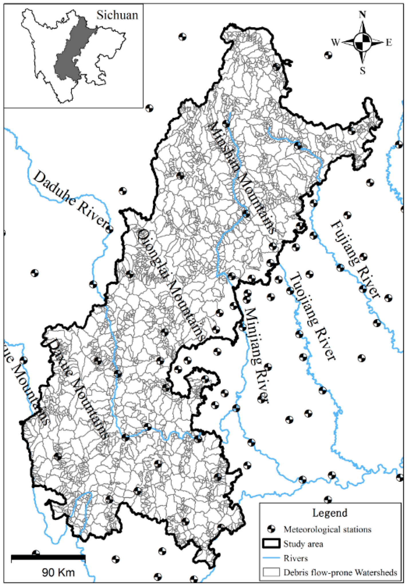
2.1. Study Area

The debris flow-prone area is a part of the Hengduan Mountains, located in the west of Sichuan Province, China (Figure 1). Covering 112,710 km2, this area is mainly comprised of hills, mountains, and a plateau while more than 95% is occupied by mountains. It is in one of the most tectonically active regions in the world. Among the historical recorded debris flow gullies, this area occupies about 48% (1575) of Sichuan province (3200). It has a subtropical monsoon climate with humid summers and dry winters. The spatial patterns of rainfall are remarkably different within the debris flow-prone area. A combination of the complex topography and monsoon climate creates a higher frequency of extreme rainfall. Meanwhile, this area is sensitive to climate change and the impacts of climate change may be profound due to the complex topography. Moreover, numerous loose deposits have been produced recently because of the 5.12 Wenchuan earthquake and the 4.20 Lushan earthquake, which have drastically increased the risk of rainfall-triggered debris flows in the study area [48,49]. For these reasons, a risk assessment of debris flow under climate change is imperative in this debris flow-prone area.

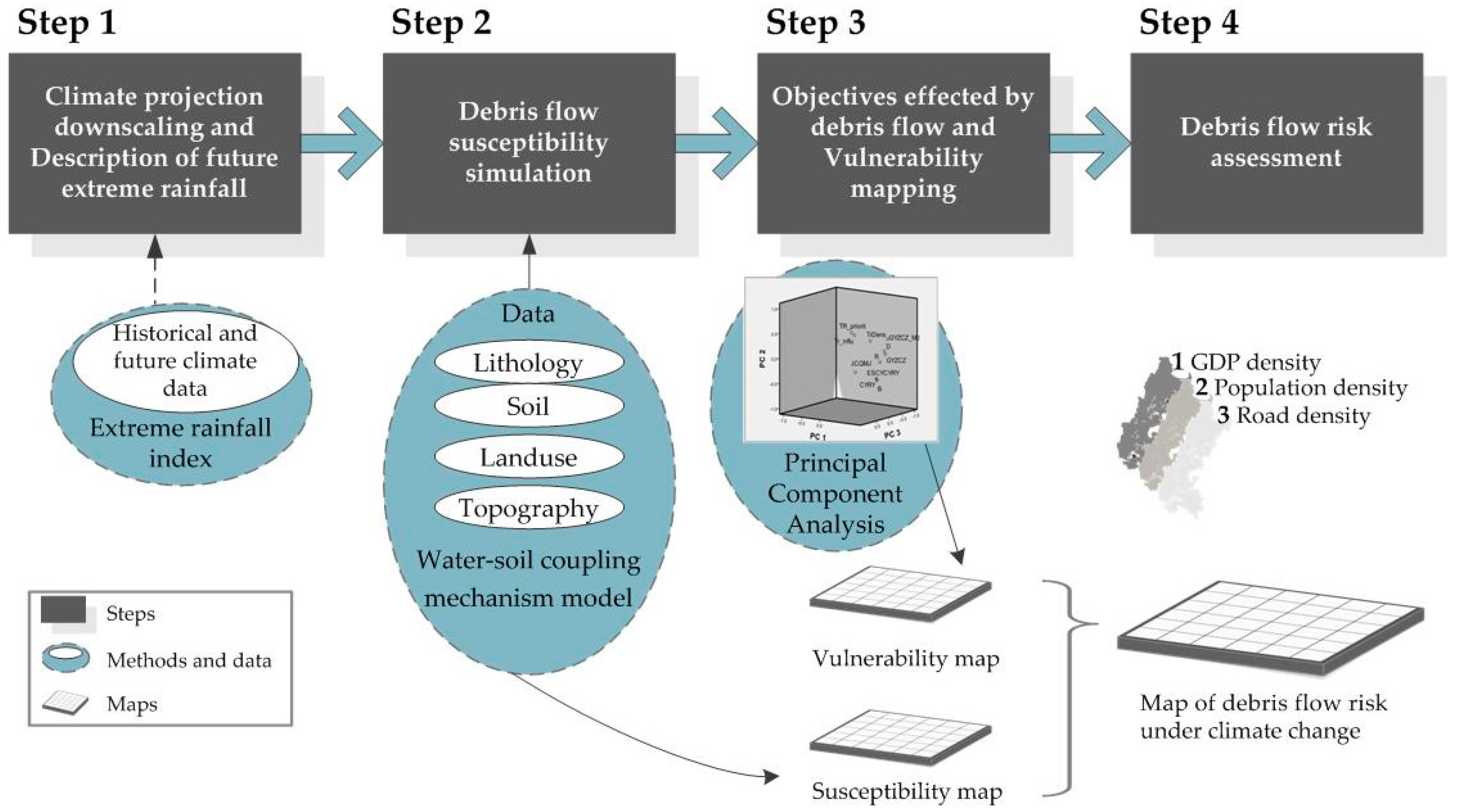
2.2. Assessment Framework

The assessment of debris flow risk was comprised of four steps, which are illustrated in Figure 2.

2.3. Models

2.3.1. Debris Flow Susceptibility

A water–soil coupling model was used for the debris flow susceptibility assessment [50]. Of all types of debris flow, shallow soil slopes sliding along bedrock is the most common in mountain areas. Furthermore, such a type is described as thick over soil failure caused by shear breakage under major exogenic forces, like precipitation, and is substantially smaller in scale, yet larger in number and greater in devastation. The formations of this type of debris flow depend on the energy, material, and triggering conditions. The relative height and terrain slope provide energy conversion gradients, while extreme rainfalls work as a triggering condition. However, it is difficult to estimate accurately the loose material of each plot for a large area. This problem can be solved by evaluating the loose material generation in each plot. In this way, the material condition of debris flow formation is influenced by geological structure, land cover, and human activity. Thus, the water–soil coupling model was established for such types of debris flow based on a geomorphology-based distributed hydrological model and the slope instability mechanism model.
The water–soil coupling process of debris flow formation can be described as having three basic steps. The first step is to simulate the surface runoff formation process. Due to the large surface slope of the mountain area and the weak river recharge of groundwater, the 1-D Richards equation set up by the finite element method was applied to present water flow in unsaturated soils for each raster, as shown in Equations (1)–(3). Surface runoff yield was based on the excess infiltration mechanism and calculated by Manning’s formula [51,52]. Secondly, based on the limit equilibrium method of infinite slopes, the slope stability alongside the instability depth under rainfall infiltration was analyzed by the safety factors calculation model as expressed in Equation (5) for each raster. If Fs < 1, the soil mass is unstable and about to transform into sediments. Third, the density of the water–soil mixture was quantified by the volume of surface runoff and the gross amount of unstable soil mass at the watershed scale. With this, a qualitative relationship between the density and probability of debris flow was presented. The density of the water–soil mixture was calculated using Equation (6):
∂θ(z, t)/∂t = (∂/∂z) × [k(θ,z) + qv(θ,z) × (∂θ/∂z)],
k(θ,z) = k0 × exp(−fz) × Se1/2 × [1 − (1 − Se1/m)m]2,
Se = (θt − θr)/(θs − θr),
Se = [1/[1 + (α × ψ)^n]]^m,
Fs = tanφ/tanβ + [c + ψ × tan(φb)]/(γt × Hs × cosβ × sinβ),
ρ = (ρw vw + ρs vs)/(vw + vs).
In Equation (1), k(θ,z) is the unsaturated soil hydraulic conductivity, and its concrete expression is shown in Equation (2). k0 is the saturated water conductivity of the surface soil layer. Se is the saturated degree as described by Equation (3). qv(θ,z) is the soil water flux. ψ = (ua − uw) is the matric suction of the soil from the Van Genuchten model of Equation (4) (ua represents the atmospheric pressure and was set to zero) [31]. n and m are the parameters of the curve, in accordance with n = 1 − 1/m. θs is the saturated water content of the soil, θr is the residual water content of the soil, and θ∆t is the soil water content of the current hour.
To calculate the safety factors in Equation (5), φ is the internal friction angle, β is the gradient, c is the soil cohesion force, φb is related to the matrix suction, γt is the wet soil density at time t, Hs is the soil depth, and Se is the same as above. In Equation (6), ρw is the density of the water (ρw = 1.0 g/cm3), and ρs is the density of solid particles (ρs = 2.7 g/cm3). vw is the volume of the water and vs is the volume of the failure soil mass.
According to these equations, the probability of debris flow can be predicted for each day in watershed units. In order to reduce uncertainties, the threshold value of the probability of debris flow was set to 0–20%, 20–40%, 40–60%, 60–80%, and 80–100%. Then, the debris flow susceptibility was expressed by the number of events for the future.

2.3.2. Vulnerability

The vulnerability of a local debris flow disaster system varies between research targets and across scales, depending on the environmental governance, demographic features, and development status [53]. In this study, vulnerability was expressed as a comprehensive index estimated through principal component analysis (PCA) and set as a range from 1 to 100. the construction of an evaluation index system is a commonly used method to integrate different categories of affected elements, to synthesize the vulnerability index by statistical methods or other mathematical methods, and to represent the relative degree of vulnerability of the assessment unit [54,55,56,57]. Considering the availability and consistency of socio-economic data in debris flow watersheds which normally correspond to the township scale, 11 variables (Table 1) were included and were mostly inferred from previous representative studies [58,59,60]. The procedures of PCA are described by Jolliffe [61]. In order to facilitate local disaster mitigation and guide decision-making, vulnerability assessment was established in the current state.
In order to tailor targeted disaster adaptation, the variables retaining a large proportion of the principal components were analyzed separately to avoid any possible unaffordable adverse impacts of debris flow. Lower vulnerability scores mean a more resilient watershed to debris flow risk.

2.3.3. Debris Flow Risk Assessment

According to the risk assessment framework [62], the debris flow risk is equal to the product of debris flow susceptibility and vulnerability as shown in Equation (7):
R = H × V

2.4. Data

The debris flow risk assessment is closely related to both natural conditions and socio-economic development level, which mainly involve datasets about precipitation, lithology, elevation, soil, land use, road, population, and GDP.

2.4.1. Daily Precipitation Data

As input data of the water–soil coupling model, daily rainfall projections were obtained from general circulation models (GCMs) of the NASA Earth Exchange Global Daily Downscaled Projections (NEX-GDDP) dataset (https://cds.nccs.nasa.gov/nex-gddp/) in RCP4.5 emissions scenarios during a time period of 2007–2060.
Since uncertainties always exist in climate projection, different GCMs can provide a more useful reference for debris flow susceptibility prediction so that the uncertainties in climate projection can be revealed and reduced. Three GCMs from CMIP5 were chosen to project future changes in precipitation, including the Beijing Climate Center Climate System Model (BCC_CCSM), the Model for Interdisciplinary Research on Climate, version 5 (MIROC5), and the Community Climate System Model version 4 (CCSM4).
Additionally, the results from NEX-GDDP could not be directly used in the water–soil coupling model due to the coarse spatial resolution (25 km × 25 km). Downscaled GCMs’ projection was capable of representing the long-term ground observations patterns. The previous literatures also indicates that downscaled GCMs have great similarity to local extreme events in the flood season [63,64]. Thus, downscaling techniques were needed to deal with raw data. In general, the local climate is closely related to land surface, elevation, and other factors. In most previous studies, linking of the statistical downscaling and spatial interpolation method was an effective approach to obtain high-resolution rainfall data [65]. In this study, the statistical downscaling approach proposed by Holland [66] was used, which used a linear correction algorithm to correct the bias of the mean climate in GCMs data. Moreover, the ANUSPLIN software was applied to interpolate the rainfall surface at a 1 km scale in terms of the bias-corrected data. Considering that an extreme rainfall event is a major driver of debris flow susceptibility, the indices of intensity, duration, and frequency were selected to analyze the differences of extreme rainfall and debris flow susceptibility.
In detail, historical data collected by the local meteorological stations in and around the debris flow-prone area (Figure 1) from 1981 to 2010 were provided by the National Meteorological Information Center of China (http://www.cma.gov.cn).

2.4.2. Environment Data

The water–soil coupling model employed multiple data, including land use, elevation (relative height and slope), surface soil, and a lithology map. Land use data were interpreted from remote sensing data of Landsat 7, 2015 (https://earthdata.nasa.gov/). A digital elevation model (DEM) of a 30-m resolution was obtained from the United States Geological Survey (https://earthexplorer.usgs.gov/). Soil datasets including soil type were provided by the institute of soil science, Chinese Academy of Sciences, and were converted into a 1 km resolution. The lithology distributions were obtained from a regional geological map while the soil cohesion, c, internal friction angle, φ, and other mechanical parameters were in accordance with a rock mechanics handbook. The relationship between the matrix suction and the soil water content was calculated by the Van Genuchten model [67]. The parameters were also determined.
All data were converted to a 100 m resolution raster in order to calculate in the assessment model.

3. Results

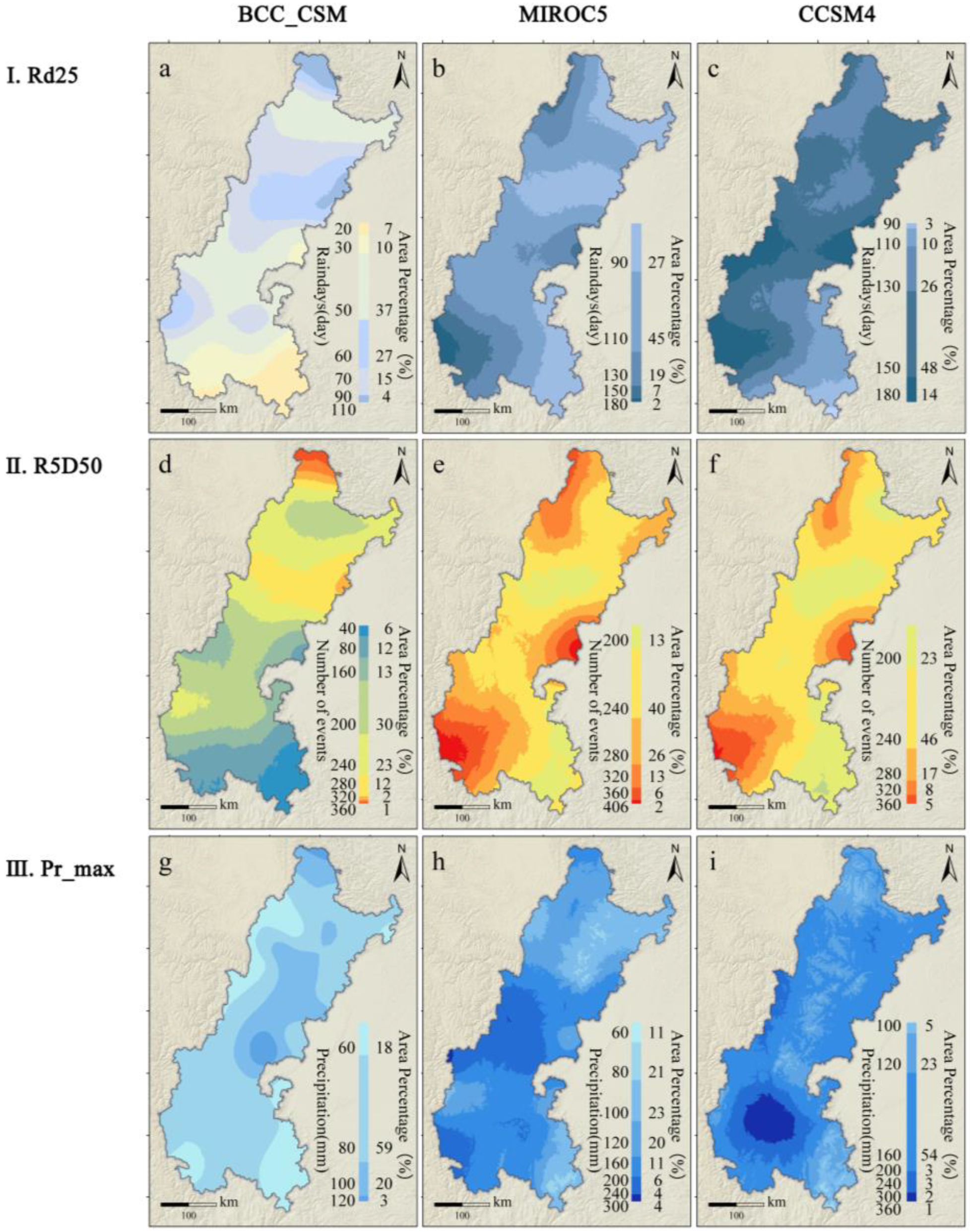
3.1. Projection of Extreme Rainfall

As shown in Figure 3, the spatial variability of extreme rainfall was rather large, as indicated by the different extreme rainfall indices. This was probably a reflection of the impacts of the complex topography and monsoons on extreme rainfall events. High frequencies of extreme rainfall were found in the transition zone from the basin to the plateau. The extreme precipitation index from BCC_CSM had larger differences, while the CCSM4 model had a higher value than the other two. Spatially, extreme rainfall was mainly concentrated in the southwest of this area. In detail, almost the whole area would experience more than 10 extreme rainfall events of Rd25 (Figure 3a–c), and about 92% of the area would contain more than 100 extreme rainfall events of R5D50 during the time period of 2007 to 2060 (Figure 3d–f). The maximum one-day precipitation ranged from less than 40 mm to more than 400 mm, while the maximum intensity was about 406 mm. About 96% of the area would experience extreme rainfall events with a total accumulated precipitation of more than 40 mm. Results from the extreme rainfall showed that areas with a maximum daily precipitation more than 50 mm are concentrated in the western part of the study area (Figure 3g–f). This suggests that the increase of extreme rainfall events would increase the possibility of debris flow events in the study areas under climate change, while the number of historical debris flow events was more than 10 in most watersheds.
Figure 3(I) presents the number of daily precipitation >25 mm (Rd25), while (a), (b), and (c) represent the indicator results of each climate model, respectively; (II) shows the number of durations of 5 days >50 mm (R5D50); and (III) presents the maximum one-day precipitation (RX1). Columns represent a corresponding model.

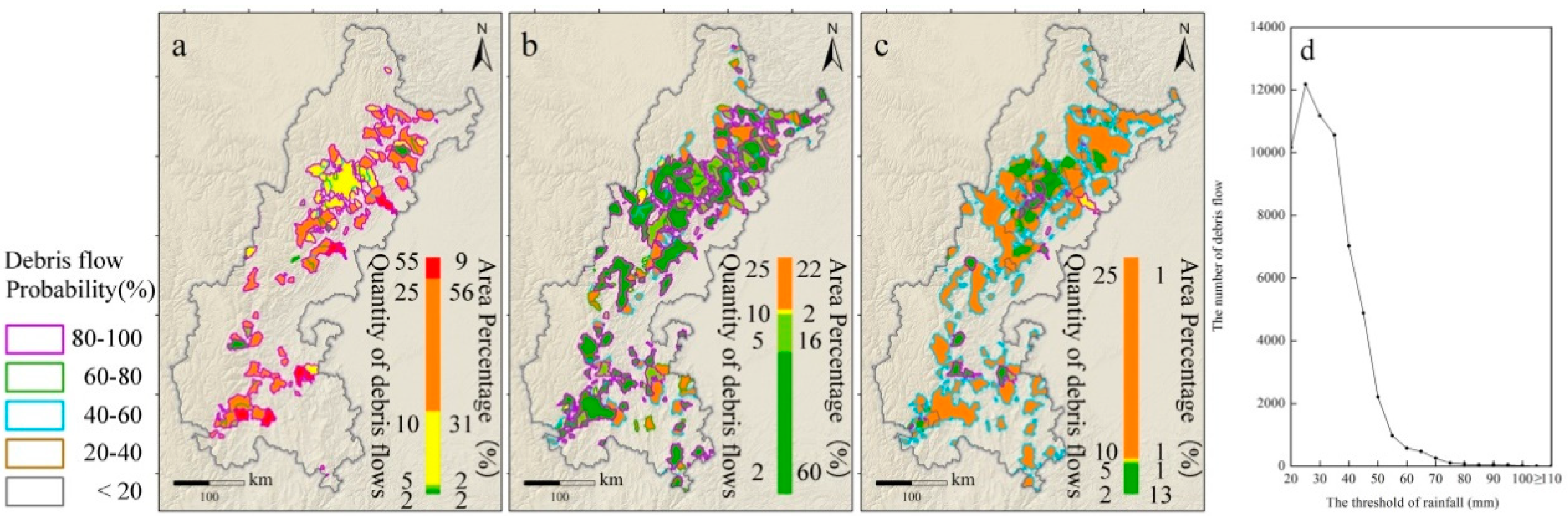
3.2. The Distribution of Debris Flow Susceptibility

Applying the water–soil coupling mechanism model to each watershed obtained results for different levels of debris flow susceptibility. Results from the BBC_CSM model showed that watersheds with a probability of debris flow above 80% had the largest range and contained those with a lower probability. Thus, watersheds with an 80% probability were used for further analysis in order to reduce uncertainties. In total, 432 of all watersheds were identified as debris flow watersheds and occupied 23% of the whole study area. High-risk areas (the number of events with debris flows >30 t) were mainly distributed in the counties of Mianzhu, Wenchuan, Leshan, and Mianning (accounting for 29% of all debris flow watersheds). As extreme rainfall events were inherently random, moderate and low-risk watersheds had greater quantities (accounting for 87% of all debris flow watersheds). Spatially, watersheds with a moderate and low-risk were more broadly distributed than high-risk watersheds, while the former were concentrated in the northern part of the study area. Additionally, the spatial distributions of potential debris flow simulated from MIROC5 and CCSM4 data were basically the same. In total, 1106 watersheds (accounting for 52%) were forecasted as debris flow watersheds. Although the hazard areas were larger, either probabilities or frequencies of future debris flow simulated by the MIROC5 and CCSM4 models were lower than the BCC_CSM model. Comparison of the distributions of extreme precipitation with the debris flow susceptibility generally showed agreement in the debris flow-prone area. However, the mechanism model helped to identify a low debris flow susceptibility under high frequencies of extreme rainfall events, such as the northwestern part of this area, by comparison between Figure 3 and Figure 4. Further analysis suggested that the rainfall threshold of debris flow varied from 30 mm to 50 mm in Figure 4d, indicating that the threshold value varies from different watersheds.

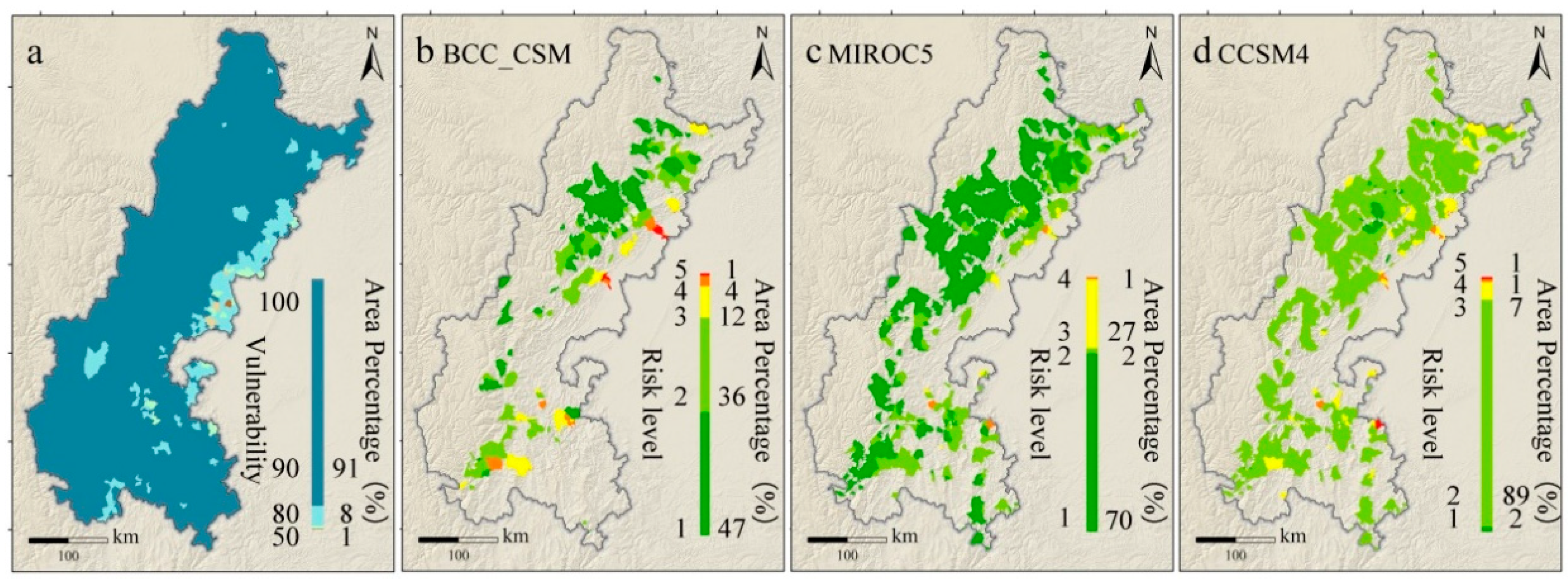
3.3. Vulnerability and Debris Flow Risk Assessment.

Three principal components were retained in PCA for the whole debris-prone area regional analysis. Together these first three principal components accounted for 73.03% of the variation in the original 11 variables included in the analysis. The factor loading was dominated by the population and workforce. The loadings of each variable for the retained principal components are detailed in Table 2.
As shown in Table 2, the first component was heavily loaded on population and workforce. The second PCA was mainly loaded on transportation related variables. The third component was loaded on production-related variables. Population density, road density, and gross domestic production with the heaviest loads of each component were thus selected for further analysis.
A measurement of vulnerability was calculated by integrating different data and was standardized to a range of 1 to 100 (Figure 5a), where higher values indicated a higher vulnerability towards debris flow. Consistent with relevant studies, the high vulnerability area towards debris flow (vulnerability value >90) comprised the most area because of the relatively low social-economic conditions in mountain areas, which accounted for over 91% of the study area. However, the level of vulnerability could also determine the debris flow risk and management strategies. Moreover, the number of debris flow events had an approximate number by comparing Figure 5c with Figure 5b. Meanwhile, the number of days with debris flows showed a significant difference between the debris flow susceptibility (Figure 4a–c) and debris flow risk (Figure 5b,c) by a paired Wilcoxon signed rank test (p < 0.05), indicating that our indices were suitable for debris flow risk assessment. As shown in Figure 5b–d, the distribution of debris flow risk showed that 53%, 30%, and 98% of debris flow watersheds would result in more than 20 times, indicating that a plan for risk management should take climate change adaptation into consideration in debris flow-prone areas.
In Figure 6, different vulnerability elements were mainly explained by the GDP, population, and road density, indicating the effects of socio-economic development on debris risk at a watershed scale. Results from the impacts of different vulnerability elements on debris flow risk showed that each selected factor could change the risk level in the study area. Meanwhile, further analysis showed that changes in one of elements were sufficient to cause the reduction in debris flow risk (Figure 5a–c). These results suggested that the improvement of socio-economic conditions was pivotal for risk management practices in the development stage of the study area.

4. Discussion

4.1. Debris Flow Process Models Enhance Susceptibility Evaluation

Compared with the approaches of debris flow risk assessment using statistical models, results from the mechanism model were more accurate in describing higher debris flow susceptibility in potential watersheds. The analysis of climate change potentially increasing the debris flow susceptibility. The differences between the mechanism and statistic model are due to the influence of environmental conditions. Although there was a simple relationship between rainfall intensity and debris flow event [68], other environmental factors, including topography, soil, and land use, are also significant drivers of debris flow [69,70,71]. Different watersheds might offer sufficient conditions to decrease the rainfall threshold, or otherwise increase debris flow susceptibility. Our results showed that the threshold ranged from 20 mm to 110 mm. According to previous studies, a rainfall intensity greater than 30 mm could trigger debris flow in the most debris flow-prone areas [72], which results in a drastic underestimate of the climate change-affected debris flow occurrences to the selection of a higher threshold value.
Rather, our results also suggested that the area of debris flow susceptibility was smaller in the whole debris-flow-prone area. Although many extreme rainfalls would occur in the future, few debris flow watersheds could be identified by the mechanism model. In consequence, a single precipitation threshold for all regions is insufficient to indicate debris flow susceptibility under climate change in risk management implementation. Applying a mechanism model may integrate different influence factors to assess debris flow susceptibility, and could reduce uncertainties arising from climate change projection and the process simulation as well.

4.2. Debris Flow Risk Reduction Management in the Future

For our study area, the rainfall threshold of rainfall-triggered debris flows had a wide range. Meanwhile, the variation in the rainfall intensity that triggered debris flow was large enough to take precautions so that differentiated risk management should be implemented in debris flow watersheds to address climate change.
Although a greater than 25 mm rainfall intensity would occur in the whole debris flow-prone area, the distribution of debris flow watersheds was mainly concentrated in the eastern part of the disaster-prone area under climate change, where the number of debris flow has increased continually in recent years [49]. Rainfall intensity, steep slope, and loose materials are pivotal factors for rainfall-triggered debris flows, which are sufficient in our debris flow watersheds. Meanwhile, previous studies suggested that the rainfall thresholds for triggering may decrease after an earthquake [73,74]. For risk reduction management under climate change, these watersheds need more attention, regardless of whether debris flows have been triggered in recent years.
Alongside the continual influence of climate change, the identification of factors of vulnerability in debris flow watersheds lays the foundation for risk assessment and management. Our results found that most of the study area showed a relatively high vulnerability to debris flow and the impacts of elements varied with debris flow watersheds. The debris flow susceptibility was assessed by the mechanism model and key factors of vulnerability were identified in each of the statistically derived watersheds, thus we were able to take different measurements for different watersheds. However, the vulnerability assessment mainly aims to serve risk reduction strategy deployment. In our study, enhancing road network density was found to be the most efficient strategy among the vulnerability factors. Moreover, the effects of the road network density could decrease the risk when the GDP decreased. Even though population density was also decreased in these watersheds, the risk was not increased rapidly. Because road density is beneficial to the circulation of regional development factors, it is regarded as the source of disaster resilience. Additionally, regional GDP also had a significant influence on the debris flow risk of watersheds at which the road density and population were at comparatively low levels. Meanwhile, rural areas have undergone rapid urbanization in China during recent decades, which has also provided opportunities for resilient community construction plans to address climate change and reduce natural hazards [75].
The integration of a debris flow mechanism model and analysis of vulnerability may be more effective for risk assessment at a watershed scale. Compared with others based on threshold values, our results highlighted the higher risk areas. Some studies suggested that moderate debris flows could also damage structures and endanger human lives [76]. Therefore, the selection result of higher risk areas would provide a more conservative strategy for risk reduction management.

5. Conclusions

In this study, it was found that integrated models which involve a debris flow mechanism model and an analysis of vulnerability may be more effective for risk assessment at a watershed scale. Results from the water–soil process model suggested that the occurrence of debris flows were more than 10 t, indicating higher debris flow susceptibility under climate change in the study area. Spatially, the risk area was mainly concentrated in the eastern part. Meanwhile, many non-debris flow watersheds were identified under climate change. Although debris flow susceptibility is the dominant factor of the increasing risk, strategies to reduce vulnerability cannot be ignored. To mitigate the impacts of debris flows under climate change, any improvement of socio-economic conditions can reduce risk on the mountainous lagging development background, among which the enhancement of road network density may be the most efficient strategy in practice.

Author Contributions

Conceptualization, Q.L. and Y.W.; Methodology, Q.L. and Y.L.; Software, Q.L. and Y.L.; Validation, Q.L.; Formal Analysis, Q.L.; Investigation, Q.L. Y.L. and P.X.; Data Curation, Y.W.; Writing—Original Draft Preparation, Q.L.; Writing—Review and editing, Q.L.; Supervision, Y.W; Project Administration, Y.L., Y.W. and P.X.; Funding acquisition, Y.W. and Y.L.

Funding

This research was funded by National Nature Science Foundation of China, grant number 41701114, and the West Light Foundation of The Chinese Academy of Sciences, grant number Y7R280080.

Acknowledgments

We wish to acknowledge the support of the following: Sichuan Provincial Development and Reform Commission for the regional disaster risk reduction under climate change cooperation. We wish to thank our colleagues in the Institute of Mountain Hazards and Environment, Chinese Academy of Sciences and Ministry of Water Resources (IMHE, CAS) for the debris flows risk management cooperation.

Conflicts of Interest

The authors declare no conflict of interest.

References

  1. Scott, K.M.; Vallance, J.W.; Kerle, N.; Macías, J.L.; Strauch, W.; Devoli, G. Catastrophic precipitation-triggered lahar at Casita volcano, Nicaragua: Occurrence, bulking and transformation. Earth Surf. Process. Landf. 2010, 30, 59–79. [Google Scholar] [CrossRef]
  2. Crozier, M.J. Deciphering the effect of climate change on landslide activity: A review. Geomorphology 2010, 124, 260–267. [Google Scholar] [CrossRef]
  3. Jakob, M.; Hungr, O.; Jakob, D.M. Debris-Flow Hazards and Related Phenomena; Springer: Chichester, UK, 2005; Volume 739. [Google Scholar]
  4. Stancanelli, L.M.; Peres, D.J.; Cancelliere, A.; Foti, E. A combined triggering-propagation modeling approach for the assessment of rainfall induced debris flow susceptibility. J. Hydrol. 2017, 550, 130–143. [Google Scholar] [CrossRef] [Green Version]
  5. Stoffel, M.; Mendlik, T.; Schneuwly-Bollschweiler, M.; Gobiet, A. Possible impacts of climate change on debris-flow activity in the Swiss Alps. Clim. Chang. 2014, 122, 141–155. [Google Scholar] [CrossRef]
  6. Stoffel, M.; Tiranti, D.; Huggel, C. Climate change impacts on mass movements—Case studies from the European Alps. Sci. Total Environ. 2014, 493, 1255–1266. [Google Scholar] [CrossRef] [PubMed]
  7. Stoffel, M.; Bollschweiler, M.; Beniston, M. Rainfall characteristics for periglacial debris flows in the Swiss Alps: Past incidences–potential future evolutions. Clim. Chang. 2011, 105, 263–280. [Google Scholar] [CrossRef]
  8. Marchi, L.; Chiarle, M.; Mortara, G. Climate changes and debris flows in periglacial areas in the Italian Alps. In Proceedings of the International Conference on from Headwaters to the Ocean: Hydrological Changes and Water Management-Hydrochange, Kyoto, Japan, 1–3 October 2008; pp. 111–115. [Google Scholar]
  9. Bardou, E.; Delaloye, R. Effects of ground freezing and snow avalanche deposits on debris flows in alpine environments. Nat. Hazards Earth Syst. Sci. 2004, 4, 519–530. [Google Scholar] [CrossRef]
  10. Stocker, T. Climate Change 2013: The Physical Science Basis: Working Group I Contribution to the Fifth Assessment Report of the Intergovernmental Panel on Climate Change; Cambridge University Press: Cambridge, UK, 2014. [Google Scholar]
  11. Acquaotta, F.; Fratianni, S.; Garzena, D. Temperature changes in the North-Western Italian Alps from 1961 to 2010. Theor. Appl. Climatol. 2015, 122, 619–634. [Google Scholar] [CrossRef]
  12. Turkington, T.; Remaître, A.; Ettema, J.; Hussin, H.; Westen, C.V. Assessing debris flow activity in a changing climate. Clim. Chang. 2016, 137, 293–305. [Google Scholar] [CrossRef] [Green Version]
  13. Davoudian, K.; Wu, J.-S.; Apostolakis, G. Incorporating organizational factors into risk assessment through the analysis of work processes. Reliab. Eng. Syst. Saf. 1994, 45, 85–105. [Google Scholar] [CrossRef]
  14. Shi, P. Disaster Risk Science; Springer: New York, NY, USA, 2018. [Google Scholar]
  15. Murray, V.; Ebi, K.L. IPCC Special Report on Managing the Risks of Extreme Events and Disasters to Advance Climate Change Adaptation (SREX); BMJ Publishing Group Ltd.: London, UK, 2012. [Google Scholar]
  16. United Nations Office for Disaster Risk Reduction. Terminology on Disaster Risk Reduction; UNDRR: Geneva, Switzerland, 2009. [Google Scholar]
  17. Winter, M.; Dent, J.; Macgregor, F.; Dempsey, P.; Motion, A.; Shackman, L. Debris flow, rainfall and climate change in Scotland. Q. J. Eng. Geol. Hydrogeol. 2010, 43, 429–446. [Google Scholar] [CrossRef]
  18. Heckmann, T.; Gegg, K.; Gegg, A.; Becht, M. Sample size matters: Investigating the effect of sample size on a logistic regression debris flow susceptibility model. Nat. Hazards Earth Syst. Sci. Discuss. 2013, 1, 2731–2779. [Google Scholar] [CrossRef]
  19. Yong-Bo, T.; Tang, C. Application of AHP in single debris flow risk assessment. Chin. J. Geol. Hazard Control 2006, 17, 79–84. [Google Scholar]
  20. Liu, G.; Li, G.; Yang, L. Risk assessments of debris flow based on improved analytic hierarchy process and efficacy coefficient method. Glob. Geol. 2012, 15, 231–236. [Google Scholar]
  21. Ning, N.; Shu, H.P.; Liu, D.F.; Jin-Zhu, M.A. Hazard assessment of debris flow based on the entropy weight method and fuzzy evaluation method. J. Lanzhou Univ. 2014, 3, 369–375. [Google Scholar]
  22. Song, S.; Zhang, B.; Feng, W.; Zhou, W. Using fuzzy relations and GIS method to evaluate debris flow hazard. Wuhan Univ. J. Nat. Sci. 2006, 11, 875–881. [Google Scholar]
  23. Liang, W.-J.; Zhuang, D.-F.; Jiang, D.; Pan, J.-J.; Ren, H.-Y. Assessment of debris flow hazards using a Bayesian Network. Geomorphology 2012, 171, 94–100. [Google Scholar] [CrossRef]
  24. Chang, T.C.; Chao, R.J. Application of back-propagation networks in debris flow prediction. Eng. Geol. 2006, 85, 270–280. [Google Scholar] [CrossRef]
  25. Marra, F.; Destro, E.; Nikolopoulos, E.I.; Zoccatelli, D.; Borga, M. Impact of rainfall spatial aggregation on the identification of debris flow occurrence thresholds. Hydrol. Earth Syst. Sci. 2017, 21, 4525–4532. [Google Scholar] [CrossRef] [Green Version]
  26. Tiranti, D.; Cremonini, R.; Asprea, I.; Marco, F. Driving factors for torrential mass-movements occurrence in the Western Alps. Front. Earth Sci. 2016, 4, 16. [Google Scholar] [CrossRef]
  27. Pudasaini, S.P. A general two-phase debris flow model. J. Geophys. Res. Earth Surf. 2012, 117, F03010. [Google Scholar] [CrossRef]
  28. Borga, M.; Dalla Fontana, G.; Cazorzi, F. Analysis of topographic and climatic control on rainfall-triggered shallow landsliding using a quasi-dynamic wetness index. J. Hydrol. 2002, 268, 56–71. [Google Scholar] [CrossRef]
  29. Peres, D.; Cancelliere, A. Estimating return period of landslide triggering by Monte Carlo simulation. J. Hydrol. 2016, 541, 256–271. [Google Scholar] [CrossRef]
  30. Salciarini, D.; Godt, J.W.; Savage, W.Z.; Baum, R.L.; Conversini, P. Modeling landslide recurrence in Seattle, Washington, USA. Eng. Geol. 2008, 102, 227–237. [Google Scholar] [CrossRef]
  31. Moscariello, A.; Marchi, L.; Maraga, F.; Mortara, G. Alluvial fans in the Italian Alps: Sedimentary facies and processes. Flood Megaflood Process. Depos. Recent Anc. Ex. 2002, 32, 141–166. [Google Scholar]
  32. Kean, J.W.; Mccoy, S.W.; Tucker, G.E.; Staley, D.M.; Coe, J.A. Runoff-generated debris flows: Observations and modeling of surge initiation, magnitude, and frequency. J. Geophys. Res. Earth Surf. 2013, 118, 2190–2207. [Google Scholar] [CrossRef]
  33. Guo, C.X.; Zhou, J.W.; Cui, P.; Hao, M.H.; Xu, F.G. A theoretical model for the initiation of debris flow in unconsolidated soil under hydrodynamic conditions. Nat. Hazards Earth Syst. Sci. Discuss. 2014, 2, 4487–4524. [Google Scholar] [CrossRef]
  34. Tiranti, D.; Crema, S.; Cavalli, M.; Deangeli, C. An integrated study to evaluate debris flow hazard in alpine environment. Front. Earth Sci. 2018, 6, 60. [Google Scholar] [CrossRef]
  35. Tiranti, D.; Deangeli, C. Modeling of debris flow depositional patterns according to the catchment and sediment source area characteristics. Front. Earth Sci. 2015, 3, 8. [Google Scholar] [CrossRef]
  36. Alvioli, M.; Melillo, M.; Guzzetti, F.; Rossi, M.; Palazzi, E.; von Hardenberg, J.; Brunetti, M.T.; Peruccacci, S. Implications of climate change on landslide hazard in Central Italy. Sci. Total Environ. 2018, 630, 1528–1543. [Google Scholar] [CrossRef]
  37. Gregoretti, C.; Degetto, M.; Boreggio, M. GIS-based cell model for simulating debris flow runout on a fan. J. Hydrol. 2016, 534, 326–340. [Google Scholar] [CrossRef]
  38. Peres, D.; Cancelliere, A. Modeling impacts of climate change on return period of landslide triggering. J. Hydrol. 2018, 567, 420–434. [Google Scholar] [CrossRef]
  39. Boberg, F.; Berg, P.; Thejll, P.; Gutowski, W.J.; Christensen, J.H. Improved confidence in climate change projections of precipitation further evaluated using daily statistics from ENSEMBLES models. Clim. Dyn. 2010, 32, 1097–1106. [Google Scholar] [CrossRef]
  40. Wisner, B.; Blaikie, P.M.; Blaikie, P.; Cannon, T.; Davis, I. At Risk: Natural Hazards, People’s Vulnerability and Disasters; Psychology Press: London, UK, 2004. [Google Scholar]
  41. Jabry, A. Children in Disasters: After the Cameras Have Gone; Plan UK: Surrey, UK, 2002. [Google Scholar]
  42. Wisner, B. Let our Children Teach us! A Review of the Role of Education and Knowledge in Disaster Risk Reduction; Inter-Agency Task Force Cluster Group on Education and Knowledge. Available online: http://www.unisdr.org/files/609_10030.pdf (accessed on 12 March 2019).
  43. Cutter, S.L.; Finch, C. Temporal and spatial changes in social vulnerability to natural hazards. Proc. Natl. Acad. Sci. USA 2008, 105, 2301–2306. [Google Scholar] [CrossRef] [PubMed] [Green Version]
  44. Bankoff, G. The historical geography of disaster: ‘Vulnerability’ and ‘local knowledge’ in western discourse. In Mapping Vulnerability; Routledge: London, UK, 2013; pp. 44–55. [Google Scholar]
  45. Cánovas, J.B.; Stoffel, M.; Corona, C.; Schraml, K.; Gobiet, A.; Tani, S.; Sinabell, F.; Fuchs, S.; Kaitna, R. Debris-flow risk analysis in a managed torrent based on a stochastic life-cycle performance. Sci. Total Environ. 2016, 557, 142–153. [Google Scholar] [CrossRef]
  46. Bardou, E.; Ancey, C.; Bonnard, C.; Vulliet, L. Classification of debris-flow deposits for hazard assessment in alpine areas. In Proceedings of the 3th International Conference on Debris-Flow Hazards Mitigation: Mechanics, Prediction, and Assessment, Davos, Switzerland, 10–12 September 2003; Millpress: Rotterdam, The Netherlands, 2003. [Google Scholar]
  47. Tiranti, D.; Bonetto, S.; Mandrone, G. Quantitative basin characterisation to refine debris-flow triggering criteria and processes: An example from the Italian Western Alps. Landslides 2008, 5, 45–57. [Google Scholar] [CrossRef]
  48. Khattak, G.A.; Owen, L.A.; Kamp, U.; Harp, E.L. Evolution of earthquake-triggered landslides in the Kashmir Himalaya, northern Pakistan. Geomorphology 2010, 115, 102–108. [Google Scholar] [CrossRef]
  49. Chang, M.; Tang, C.; Van Asch, T.W.; Cai, F. Hazard assessment of debris flows in the Wenchuan earthquake-stricken area, South West China. Landslides 2017, 14, 1783–1792. [Google Scholar] [CrossRef]
  50. Zhang, S.; Yang, H.; Wei, F.; Jiang, Y.; Liu, D. A model of debris flow forecast based on the water-soil coupling mechanism. J. Earth Sci. 2014, 25, 757–763. [Google Scholar] [CrossRef]
  51. Manning, R.; Griffith, J.P.; Pigot, T.; Vernon-Harcourt, L.F. On the flow of water in open channels and pipes. Trans. Inst. Civ. Eng. Irel. 1891, 20, 161–207. [Google Scholar]
  52. Schetz, J.A.; Fuhs, A.E. Fundamentals of Fluid Mechanics; John Wiley & Sons: New York, NY, USA, 1999. [Google Scholar]
  53. Ding, M.; Heiser, M.; Hübl, J.; Fuchs, S. Regional vulnerability assessment for debris flows in China—A CWS approach. Landslides 2016, 13, 537–550. [Google Scholar] [CrossRef]
  54. Kaźmierczak, A.; Cavan, G. Surface water flooding risk to urban communities: Analysis of vulnerability, hazard and exposure. Landsc. Urban Plan. 2011, 103, 185–197. [Google Scholar] [CrossRef]
  55. Shirley, W.L.; Boruff, B.J.; Cutter, S.L. Social vulnerability to environmental hazards. In Hazards Vulnerability and Environmental Justice; Routledge: London, UK, 2012; pp. 143–160. [Google Scholar]
  56. Cutter, S.L. Vulnerability to environmental hazards. In Hazards Vulnerability and Environmental Justice; Routledge: London, UK, 2012; pp. 99–110. [Google Scholar]
  57. Moss, R.H.; Brenkert, A.L.; Malone, E.L. Vulnerability to Climate Change: A Quantitative Approach; Prepared for the US department of energy; PNNL-SA-33642; Pacific Northwest National Laboratory: Richland, WA, USA, 2001; pp. 155–167.
  58. Jin, F.; Wang, C.; Li, X.; Wang, J. China’s regional transport dominance: Density, proximity, and accessibility. J. Geogr. Sci. 2010, 20, 295–309. [Google Scholar] [CrossRef]
  59. Santi, P.; Hewitt, K.; Van Dine, D.; Cruz, E.B. Debris-flow impact, vulnerability, and response. Nat. Hazards 2011, 56, 371–402. [Google Scholar] [CrossRef]
  60. Ciurean, R.; Hussin, H.; Van Westen, C.; Jaboyedoff, M.; Nicolet, P.; Chen, L.; Frigerio, S.; Glade, T. Multi-scale debris flow vulnerability assessment and direct loss estimation of buildings in the Eastern Italian Alps. Nat. Hazards 2017, 85, 929–957. [Google Scholar] [CrossRef]
  61. Jolliffe, I. Principal Component Analysis; Springer: New York, NY, USA, 2011. [Google Scholar]
  62. Pelling, M.; Maskrey, A.; Ruiz, P.; Hall, P.; Peduzzi, P.; Dao, Q.-H.; Mouton, F.; Herold, C.; Kluser, S. Reducing Disaster Risk: A Challenge for Development; United Nations: New York, NY, USA, 2004. [Google Scholar]
  63. Sillmann, J.; Kharin, V.; Zwiers, F.; Zhang, X.; Bronaugh, D. Climate extremes indices in the CMIP5 multimodel ensemble: Part 2. Future climate projections. J. Geophys. Res. Atmos. 2013, 118, 2473–2493. [Google Scholar] [CrossRef]
  64. Ying, X.; Bing, Z.; Bo-Tao, Z.; Si-Yan, D.; Li, Y.; Rou-Ke, L. Projected flood risks in China based on CMIP5. Adv. Clim. Chang. Res. 2014, 5, 57–65. [Google Scholar] [CrossRef]
  65. Hijmans, R.J.; Cameron, S.E.; Parra, J.L.; Jones, P.G.; Jarvis, A. Very high resolution interpolated climate surfaces for global land areas. Int. J. Climatol. 2005, 25, 1965–1978. [Google Scholar] [CrossRef]
  66. Holland, G.; Done, J.; Bruyere, C.; Cooper, C.K.; Suzuki, A. Model investigations of the effects of climate variability and change on future Gulf of Mexico tropical cyclone activity. In Proceedings of the Offshore Technology Conference, Houston, TX, USA, 3–6 May 2010. [Google Scholar]
  67. Van Genuchten, M.T. A closed-form equation for predicting the hydraulic conductivity of unsaturated soils 1. Soil Sci. Soc. Am. J. 1980, 44, 892–898. [Google Scholar] [CrossRef]
  68. Pan, H.-L.; Jiang, Y.-J.; Wang, J.; Ou, G.-Q. Rainfall threshold calculation for debris flow early warning in areas with scarcity of data. Nat. Hazards Earth Syst. Sci. 2018, 18, 1395–1409. [Google Scholar] [CrossRef] [Green Version]
  69. Roberson, C.; Das, D.K. Debris Flow: Mechanics, Prediction and Countermeasures; CRC Press: Boca Raton, FL, USA, 2014. [Google Scholar]
  70. Scheidl, C.; Rickenmann, D. Empirical prediction of debris-flow mobility and deposition on fans. Earth Surf. Process. Landf. 2010, 35, 157–173. [Google Scholar] [CrossRef]
  71. Turconi, L.; De, S.K.; Tropeano, D.; Savio, G. Slope failure and related processes in the Mt. Rocciamelone area (Cenischia valley, Western Italian Alps). Geomorphology 2010, 114, 115–128. [Google Scholar] [CrossRef]
  72. Pelfini, M.; Santilli, M. Frequency of debris flows and their relation with precipitation: A case study in the Central Alps, Italy. Geomorphology 2008, 101, 721–730. [Google Scholar] [CrossRef]
  73. Chiou, S.-J.; Cheng, C.-T.; Hsu, S.-M.; Lin, Y.-H.; Chi, S.-Y. Evaluating landslides and sediment yields induced by the Chi-Chi Earthquake and followed heavy rainfalls along the Ta-Chia River. J. GeoEng. 2007, 2, 73–82. [Google Scholar]
  74. Tang, C.; Zhu, J.; Chang, M.; Ding, J.; Qi, X. An empirical–statistical model for predicting debris-flow runout zones in the Wenchuan earthquake area. Quat. Int. 2012, 250, 63–73. [Google Scholar] [CrossRef]
  75. Liu, Y. Introduction to land use and rural sustainability in China. Land Use Policy 2018, 74, 1–4. [Google Scholar] [CrossRef]
  76. Iverson, R.M. The physics of debris flows. Rev. Geophys. 1997, 35, 245–296. [Google Scholar] [CrossRef] [Green Version]
Figure 1. Study area showing the distribution of 2136 selected debris flow-prone watersheds.
Sustainability 11 03199 g001
Figure 2. Illustration of the risk assessment approach via a flow chart.
Sustainability 11 03199 g002
Figure 3. The distributions of extreme precipitation under climate change in the future.
Sustainability 11 03199 g003
Figure 4. (ac) show the spatial distribution of the number of debris flow events with different levels of probability for the BCC_CSM, MIROC5, and CCSM4 models, respectively. (d) shows the triggering threshold of rainfall in the disaster-prone-area.
Sustainability 11 03199 g004
Figure 5. The spatial distributions of vulnerability under the current regional development condition and debris flow risk under different GCMs.
Sustainability 11 03199 g005
Figure 6. The impacts of different elements on debris flow risk under climate change. (ac) represent GDP, population density, and road density, respectively.
Sustainability 11 03199 g006
Table 1. Summary of the variables used in the comprehensive vulnerability index.
VariablesDescriptionMethods and Source
Population density Dpop = P/S
Non-agricultural work forceThe number of people engage in work other than agriculture, i.e., industrial and service employeesCensus data (2014)
GDPGross domestic productCensus data (2014)
Town-constructed areaArea of regions with complete infrastructure facility and public utilities in townCensus data (2014)
Industrial production density Dip = V/S
Workforce quantity Census data (2014)
population proportionThe proportion of population of a certain town to that of the superior countyB = P/P0
Population concentrationThe relative importance of population distribution for a certain townR = B/(S/S0)
Traffic net density Dti = Lti/S
Traffic trunk influenceInfluence of different types of traffic trunk linesf(xi) = C11 + C12 + … + Cim i ∈ (1, 2, 3, …, n) m ∈ (1, 2, 3, …, M)
Primacy indexPrimacy index means the transportation radiation force of a primate city and represents the social and economic conditions of towns been affected by the primate cities.lef (x) = ∑(n → u = 1) lefu
fef (x) = min (lef (x))
   = min (∑(n → u = 1) lefu) e
   = (1, 2, 3, …, n)
fe (x) = mine (fef (x))
   = mine (min (∑(n → u = 1) lefu) e)
e = (1, 2, 3, …, n)
He ∈ {Hf} He {0,1}
parameters
Dpop—density of population, P—the permanent population of a town, P0—the permanent population of a county
Dip—density of industrial production, V—annual industrial production, S—Town area, S0—county area
Dti—density of traffic network, Lti—line length or traffic nodes of traffic network
Cim—influence of m traffic trunk lines, I—traffic type (Roads, railways, airports, etc.), m—traffic trunk level
u—minimum line length from e to f. If lef ≤ 100 km, traffic type is set to roads, otherwise railways.
Then, the shortest path function, fe (x), is determined by comparing the minimum value of the path from the primate city to region e.
According to the function, an important node, f, is selected as a junction node for region e.
Hi is a Boolean value. When the fe (x) function is true, Hi is 1 or vice versa.
Using the function in a GIS software, the hinterland range of the important node, f, Hm (i) is defined through search and comparison.
Table 2. Retained principal components of vulnerability.
PC1PC2PC3
Population density0.901−0.3330.191
Town population proportion0.901−0.3320.192
Non-agricultural work force0.884−0.370.138
Population concentration0.864−0.033−0.001
Primacy index0.390.5780.444
Traffic trunk influence0.4680.5330.436
Industrial production density0.5910.304−0.691
GDP0.7150.05−0.419
Traffic net density0.6040.3680.004
workforce0.8190.153−0.232
Extraction methods: Principal component analysis.
a. Three components extracted

