

The Effect of Error Non-Orthogonality on Triple Collocation Analyses

Royal Netherlands Meteorological Institute KNMI, Utrechtseweg 297, 3731 GA De Bilt, The Netherlands
*
Author to whom correspondence should be addressed.
Remote Sens. 2022, 14(17), 4268; https://doi.org/10.3390/rs14174268
Submission received: 4 July 2022
/
Revised: 25 August 2022
/
Accepted: 26 August 2022
/
Published: 30 August 2022
(This article belongs to the Special Issue Remote Sensing of Ocean Surface Winds)
Abstract
:Triple collocation analysis is an established technique for calculating the relative linear intercalibration coefficients and observation error variances for physical quantities measured simultaneously in space and time by three different observation systems. A simple parameterized error model is used. It relies on a few assumptions, one of which is that the observation errors are independent of the magnitude of the observed quantities. This is referred to as error orthogonality. Using an ocean surface vector winds data set of 44,948 collocations, this study shows that the violation of error orthogonality does affect the calibration coefficients but has only a small second-order effect on the observation error variances of the calibrated data.
1. Introduction
Triple collocation is a powerful technique for calculating the observation error variances and linear intercalibration coefficients of a physical quantity measured by three different observation systems at the same time and place. It was introduced by Stoffelen [1] for ocean surface vector winds and later applied by [2] to estimate the accuracy of high-resolution scatterometer wind products. In the past years the technique has been applied on an increasing number of geophysical quantities like ocean surface wind speed [3], ocean surface current [4], sea surface salinity [5], precipitation [6,7], soil moisture [8,9], groundwater storage [10], etc. The list of references is far from complete, and the interested reader is referred to the references and the references therein.
Triple collocation has been extended to include a generalization of the correlation coefficient known from linear regression analysis [11]. Extensions to more than three collocated measurement systems have also been proposed [4,12], but these fall outside the scope of this paper.
Triple collocation relies on the following assumptions:
- (1)
- Linear calibration is sufficient to describe the interrelations between the observation systems;
- (2)
- The observation errors are random with zero average after calibration;
- (3)
- The observation errors are independent of the measured value (error orthogonality).
When deriving the triple collocation equations, one usually applies all approximations as soon as possible in order to simplify the algebra, arguing that the sufficiency of linear calibration can be judged from scatter plots and that error orthogonality is hard to check. To the best of the authors’ knowledge, the effect of violation of error orthogonality (further referred to as error non-orthogonality) has never been tested. The aim of this short paper is to fill this gap. It will be shown that error non-orthogonality can be included in the triple collocation covariance equations in an elegant and concise manner. The effect of error non-orthogonality will be studied for a data set consisting of all buoy, OSCAT-25, and European Centre for Medium-Range Weather Forecasts (ECMWF) atmospheric reanalysis ERA5 forecast collocations in 2013 [12,13].
The paper is organized as follows. Section 2 contains a brief description of the data used. In Section 3 error orthogonality is included in the covariance equations for triple collocation analysis. Representativeness errors are defined and included, and the method of solution is briefly described. The results are presented and discussed in Section 4. The paper ends with the conclusions in Section 5.
2. Data
The data set used in this work consists of 44,948 collocations of buoy surface winds data obtained from ECMWF’s archive, called Meteorological Archival and Retrieval System (MARS), reprocessed OSCAT winds on a 25 km grid, and ERA5 forecast winds, all in 2013. OSCAT is a rotating pencil-beam Ku-band scatterometer carried by the Oceansat-2 satellite operated by the Indian Space Research Organization (ISRO). Oceansat-2 was launched 23 September 2009, and delivered data from 16 December 2009 until instrument breakdown on 14 February 2014. The data were reprocessed in 2021 at KNMI with the Pencil-beam Wind data Processor (PenWP) and collocated with the buoy and ERA-5 forecasts. The ERA5 forecasts were interpolated quadratically in time and bilinear in space to the time and position of the OSCAT measurements. The forecasts had a minimum lead time of three hours to avoid using forecasts in which the OSCAT data were assimilated. The collocation criteria were a maximum difference of 30 min in time and 17.7 km ( times the grid size) in position for the buoy and OSCAT measurements. See [14] for more information.
3. Methodology
3.1. Triple Collocation with Error Non-Orthogonality
The error model employed here is the canonical model
where is the measurement by system , , the calibration scaling, the calibration bias, the common signal measured by all three systems (also referred to as “truth”, but that term may be misleading as is determined by the system with coarsest resolution), and a random measurement error with zero average and variance .
If consists of a constant part and a -dependent part , , the -dependent part will be added to in the error model (1). Compared with the other systems, the calibration of system will appear different because the dependency to has changed. The error model thus implicitly removes error non-orthogonality, and it is not possible to retrieve from it. As a consequence, any information on error non-orthogonality must come from other sources.
Without loss of generality, system 1 can be chosen as the reference system relative to which systems 2 and 3 will be calibrated, so and .
Taking first moments (averages) , where the brackets stand for taking the average (arithmetic mean) over all measurements, one obtains
since because the random measurement errors have zero mean. Since and , Equation (2) implies that
Substituting this back in Equation (2) yields
so that the calibration biases and are known once we know the calibration scalings.
To find the calibration scalings and the error variances one must take second moments :
The terms with averaging brackets 〈 〉 are handled as follows. From Equation (3) it follows that . Further
where and . Note that when the errors do not depend on the measured value, the usual assumption. In the literature this is called error orthogonality, so let’s call the error non-orthogonality of system . Further, note that . The calibration biases are removed by substituting Equation (4), and the result is
Introducing covariances and common variance , Equation (7) yields the covariance equations
The usual form of the covariance equations is . In Equation (8), two extra terms appear because the approximation of error orthogonality was not made. It should be noted here that the covariances are not unbiased; they can be made unbiased by multiplying them by a factor , with the number of collocations. When is large, as is the case in this study with 44,948 collocations, the factor can safely be neglected.
For triple collocation, the error variances follow from the three diagonal covariance equations as
The three off-diagonal equations read
Equations (10a)–(10c) are usually solved by assuming , and the solution reads
From Equations (10a)–(10c), it is clear that error non-orthogonality’s and error covariances will affect the calibration scalings and common variance, and this may in turn affect the error variances.
3.2. Representativeness Errors
If the spatial, temporal or geophysical representation of the three systems is different, representativeness errors must be taken into account [1,2,15]. Suppose that the systems are ordered in decreasing spatial resolution with system 1 the buoys (calibration reference), system 2 the scatterometer, and system 3 the ERA-5 forecasts. Then systems 1 and 2 will measure a common signal that is not observed by system 3 because of its coarser resolution. This common signal is called the representativeness error or, sometimes, the representativeness signal. It will appear as an error correlation in Equation (10a). The representativeness errors in this study are estimated from differences in spatial variances [15,16]. For the OSCAT and ERA5 data mentioned above, they are 0.181 m2 s−2 for the zonal wind component and 0.145 m2 s−2 for the meridional wind component .
3.3. Method of Solution
The triple collocation Equations (9) and (10) are solved in an iterative algorithm that starts by assuming that the systems are well intercalibrated. In each iteration the covariances are recalculated using the calibration coefficients from the previous iteration (or their starting values for the first iteration). Then the calibration coefficients are updated and outliers may be removed, see [15] for more details. The iteration converges in about 7 steps. The final values for the observation error variances are for the calibrated data; those for the uncalibrated data can be obtained by dividing by .
As representativeness errors and error non-orthogonalities must be obtained from other sources than the triple collocation analysis itself, they can be moved to the left-hand side of Equations (10a)–(10c), so the covariance Equation (8) become
With the replacement
the covariance equations can be solved as usual. In the solution scheme employed here, the calibration coefficients are known in each iteration, at least approximately, so the replacement Equation (13) can be applied without problems. Therefore, the effect of error non-orthogonalities can be studied in the same way as that of representativeness errors or error correlations by incorporating them in the covariances in each iteration step.
4. Results and Discussion
The effect of error non-orthogonality is studied by assuming that one of the observation systems contains an error non-orthogonality that ranges from −1 m2 s−2 to +1 m2 s−2, a range that is considerable with respect to the representativeness errors and the error variances. This is repeated for all three systems.
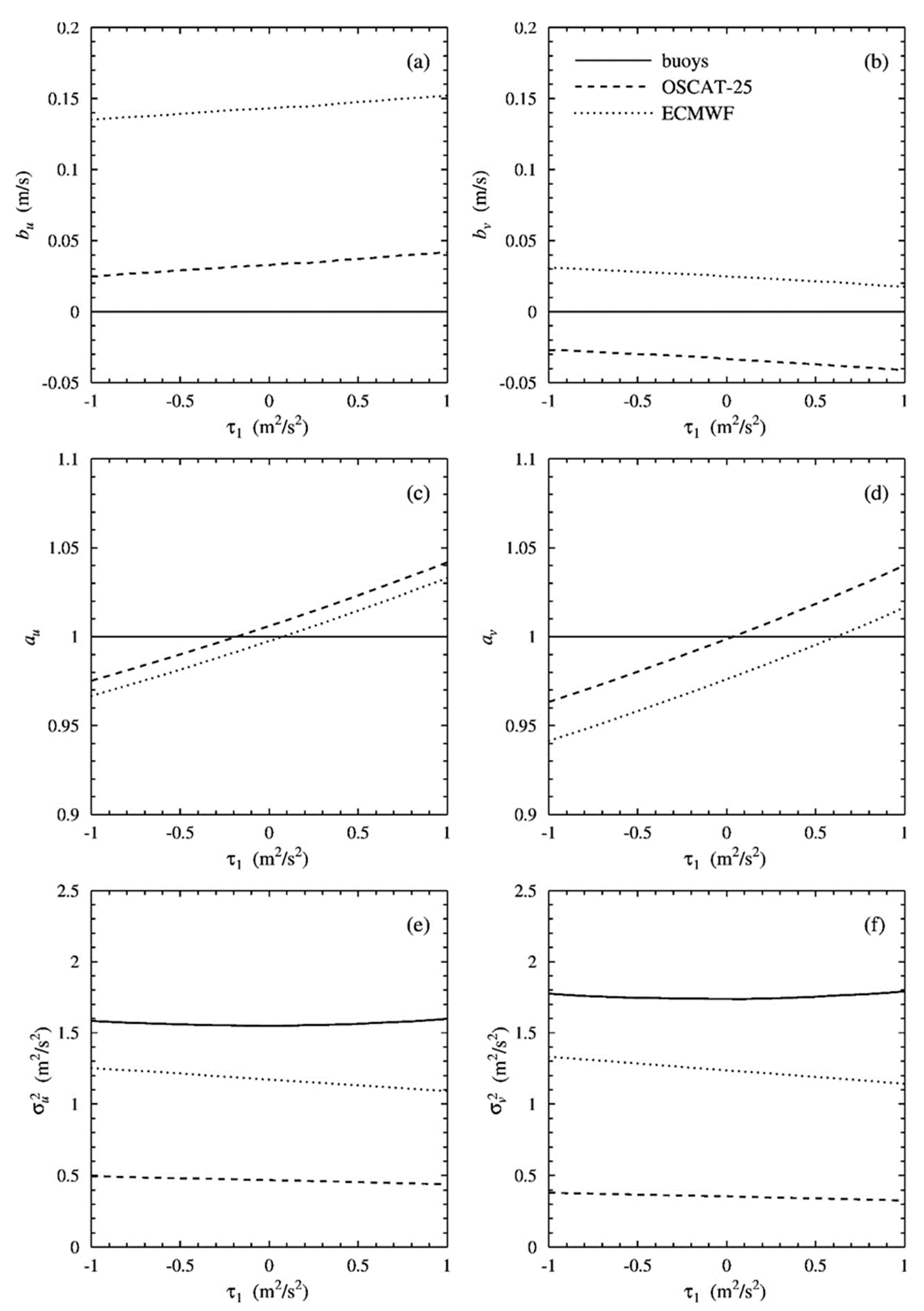
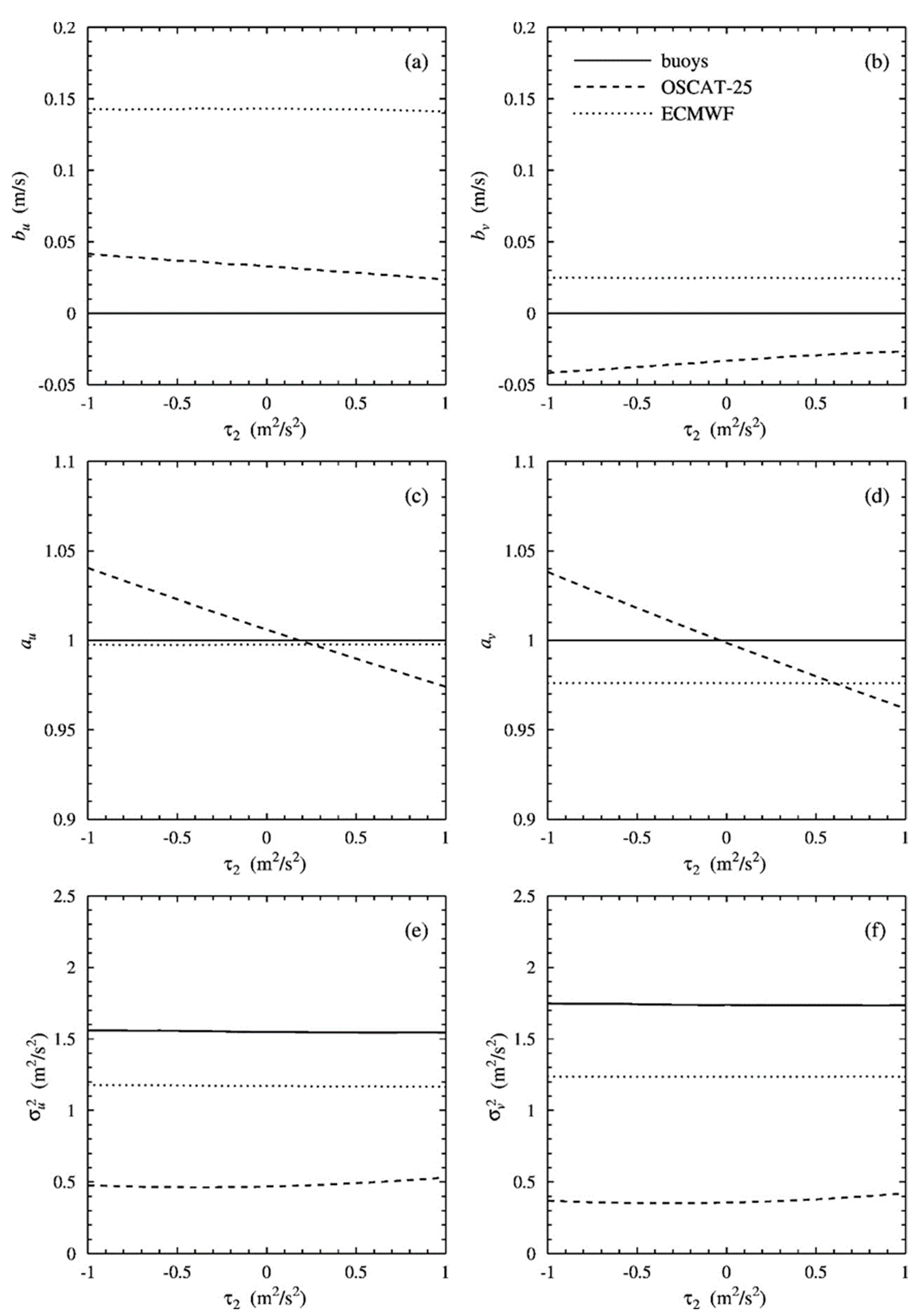
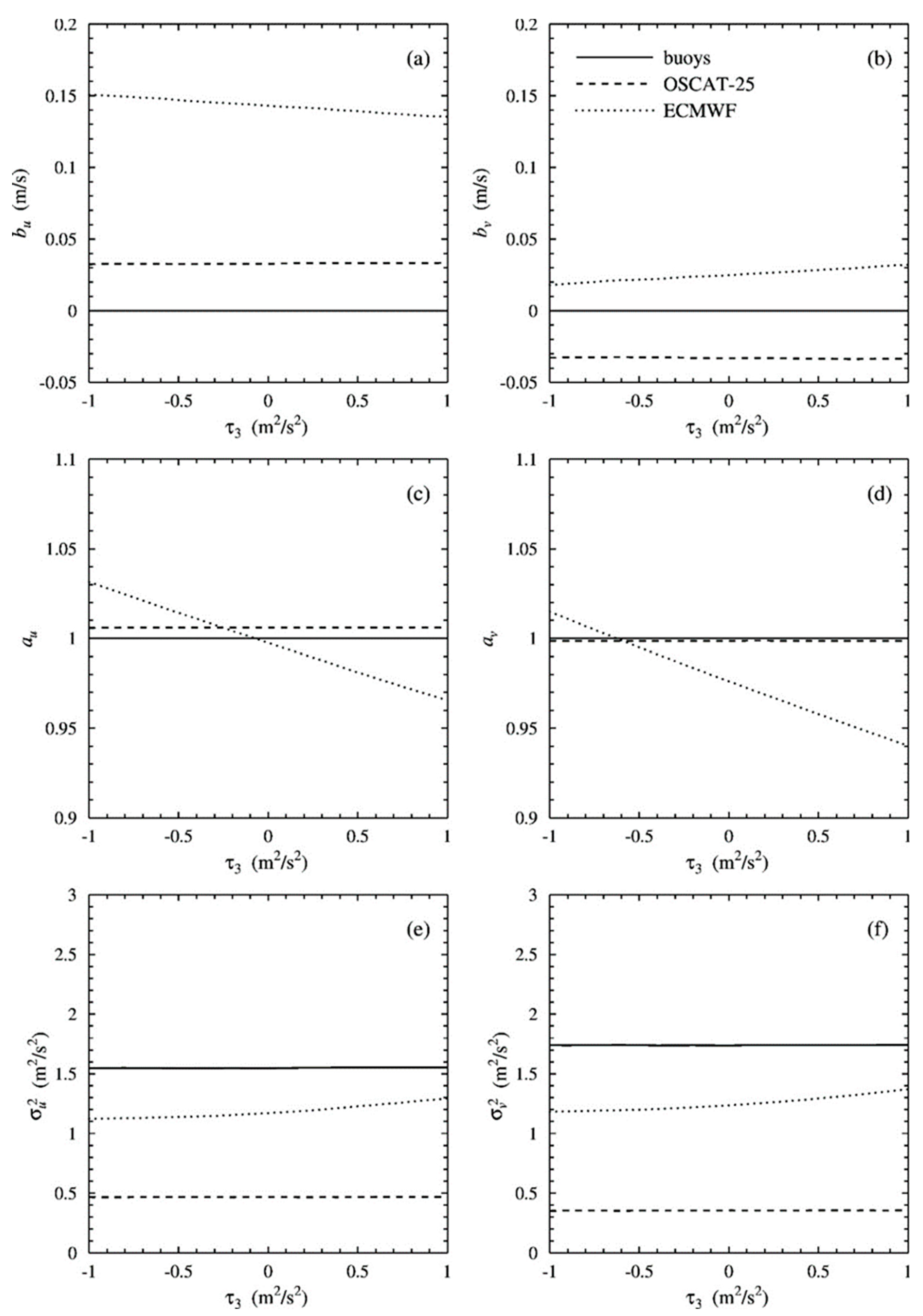
Figure 1a,b show the effect of error non-orthogonality in the buoys, τ1, on the calibration biases, Figure 1c,d that on the calibration scalings, and Figure 1e,f that on the observation error variances for the zonal wind component (Figure 1a,c,e) and the meridional wind component (Figure 1b,d,f). Figure 2 and Figure 3 are similar to Figure 1, but for error non-orthogonality in OSCAT and in the ECMWF forecast, and , respectively. The figures show results for the observation error variances of the calibrated data.
In all figures, the calibration biases are only weakly affected by error non-orthogonality. Note that the calibration bias of the buoys equals 0 as they were selected as calibration reference. The effect on the bias depends on the dynamic range of and hence differs for and .
More effect of error non-orthogonality can be seen in the calibration scalings, as expected. For error non-orthogonality in the buoys (Figure 1), the scaling of both scatterometer and ECMWF increases with increasing , while for error non-orthogonality in the scatterometer (Figure 2) or in the ECMWF forecasts (Figure 3), the calibration scaling of the system having error non-orthogonality decreases with , the other systems being unaffected.
This can be summarized as that error non-orthogonality only reduces the calibration scaling of the system having it. If that system happens to be the calibration reference, as in Figure 1, it will lift the other calibration scalings.
The most surprising in Figure 1, Figure 2 and Figure 3 is that the observation error variances are only very weakly affected by error non-orthogonality. Apparently, the effects of in Equations (9) and (10) largely cancel, and this can be understood by making a first-order Taylor expansion of the observation error variances in ,
For example, let . From Equation (14) one readily finds that
Now the off-diagonal covariances are all equal to each other when the triple collocation algorithm has converged, because then the calibration scalings are all equal to 1. Therefore is independent of to first order, and only dependencies of second and higher order remain. Similarly,
and the linear dependency of on vanishes because of the equality of the off-diagonal covariances. Finally,
because follows from by replacing with and interchanging and . The linear dependencies of , , and on and can be shown to vanish in the same manner.
It must be stressed here that the observation error variances are for the calibrated data. To retrieve the observation error variances in the uncalibrated data one must divide by . As a result, the observation error variances of the uncalibrated data do depend on error non-orthogonality in a manner opposite to the calibration scalings.
5. Conclusions
Error non-orthogonality is included in an elegant and concise manner in the covariance equations for triple collocation. The formalism is applied on a data set consisting of all collocated wind velocities in 2013 from buoys, OSCAT-25, and ECMWF forecasts. Varying the error non-orthogonality of each system separately shows only weak dependence for the calibration biases and, in particular, the observation error variances. The observation error variances are sensitive to error non-orthogonality only in second and higher order. This implies that error non-orthogonality cannot be blamed for possible unexpected observation error variances from triple collocation analyses of ocean surface vector winds. Only the calibration scalings show a strong dependency on error non-orthogonality. The calibration scaling of the system with error non-orthogonality decreases with increasing , except for the reference system where the calibration scalings of all other systems will increase with increasing . This implies that error non-orthogonality is aliased with calibration error in scatter plots, at least qualitatively and for relatively large , where the calculated regression line deviates from the diagonal in the cloud of observed points for both cases.
Because of the generality of the covariance equations, as for higher-order collocations as elaborated in [15] as well, error non-orthogonality can also be studied for quadruple and higher-order collocations. However, the results are expected not to differ much from the results presented here.
Author Contributions
Conceptualization and methodology, J.V. and A.S.; software, J.V.; validation, J.V.; formal analysis, J.V.; investigation, J.V.; resources, A.S.; data curation, A.V.; writing—original draft preparation, J.V.; writing—review and editing, J.V., A.S., and A.V.; visualization, J.V.; supervision, A.S.; project administration, A.S. and A.V.; funding acquisition, A.S. and A.V. All authors have read and agreed to the published version of the manuscript.
Funding
This work has been funded by EUMETSAT within the framework of the Ocean and Sea Ice Satellite Application Facility (OSI SAF).
Data Availability Statement
The collocation data set can be obtained from the authors upon a request to [email protected]. The PenWP source code can be downloaded free of charge at https://nwp-saf.eumetsat.int/site/software/scatterometer/penwp/ (accessed on 25 August 2022). A simple free triple collocation code in Python can be found at https://github.com/knmiscat/triple_collocation (accessed on 25 August 2022).
Acknowledgments
The authors thank Jean Bidlot of ECMWF for his assistance in obtaining the buoy data and Weicheng Ni of the National University of Defense Technology in China for his interest in this work and stimulating discussions.
Conflicts of Interest
The authors declare no conflict of interest. The funder had no role in the design of the study; in the collection, analysis, or interpretation of data; in the writing of the manuscript; or in the decision to publish the results.
References
- Stoffelen, A. Toward the True Near-surface Wind Speed: Error Modelling and Calibration using Triple Collocation. J. Geophys. Res. 1998, 103, 7755–7766. [Google Scholar] [CrossRef]
- Vogelzang, J.; Stoffelen, A.; Verhoef, A.; Figa-Saldaña, J. On the Quality of High-resolution Scatterometer Winds. J. Geophys. Res. 2011, 116, C10033. [Google Scholar] [CrossRef]
- Abdalla, S.; De Chiara, G. Estimating Random Errors of Scatterometer, Altimeter, and Model Wind Speed Data. IEEE J. Sel. Top. Appl. Earth Obs. Remote Sens. 2017, 10, 2406–2414. [Google Scholar] [CrossRef]
- Danielson, R.E.; Johannessen, J.A.; Quartly, G.D.; Rio, M.-H.; Chapron, B.; Collard, F.; Donlon, C. Exploitation of Error Correlation in a Large Analysis Validation: GlobCurrent Case Study. Rem. Sens. Env. 2018, 217, 476–490. [Google Scholar] [CrossRef]
- Hoareau, N.; Portabella, M.; Lin, W.; Ballabrera-Poy, J.; Turiel, A. Error Characterization of Sea Surface Salinity Products using Triple Collocation Analysis. IEEE Trans. Geosci. Remote Sens. 2018, 56, 5160–5168. [Google Scholar] [CrossRef]
- Roebeling, R.A.; Wolters, E.L.A.; Meirink, J.F.; Leijnse, H. Triple Collocation of Summer Precipitation Retrievals from SEVIRI over Europe with Gridded Rain Gauge and Weather Radar Data. J. Hydrometeorol. 2012, 13, 1552–1566. [Google Scholar] [CrossRef]
- Wild, A.; Chua, Z.-W.; Kuleshov, Y. Triple Collocation Analysis of Satellite Precipitation Estimates over Australia. Remote Sens. 2022, 14, 2724. [Google Scholar] [CrossRef]
- Gruber, A.; Su, C.-H.; Crow, W.T.; Zwieback, S.; Dorigo, W.A.; Wagner, W. Estimating Error Cross-correlations in Soil Moisture Data Sets using Extended Collocation Analysis. J. Geophys. Res. Atmos. 2016, 121, 1208–1219. [Google Scholar] [CrossRef]
- Fan, X.; Lu, Y.; Liu, Y.; Li, T.; Xun, S.; Zhao, X. Validation of Multiple Soil Moisture Products over an Intensive Agricultural Region: Overall Accuracy and Diverse Responses to Precipitation and Irrigation Events. Remote Sens. 2022, 14, 3339. [Google Scholar] [CrossRef]
- Su, K.; Zheng, W.; Yin, W.; Hu, L.; Shen, Y. Improving the Accuracy of Groundwater Storage Estimates Based on Groundwater Weighted Fusion Model. Remote Sens. 2022, 14, 202. [Google Scholar] [CrossRef]
- McColl, K.A.; Vogelzang, J.; Konings, A.G.; Entekhabi, D.; Piles, M.; Stoffelen, A. Extended triple collocation: Estimating Errors and Correlation Coefficients with respect to an Unknown Target. Geophys. Res. Lett. 2014, 41, 6229–6236. [Google Scholar] [CrossRef]
- Hersbach, H.; Bell, B.; Berrisford, P.; Hirahara, S.; Horányi, A.; Muñoz-Sabater, J.; Nicolas, J.; Peubey, C.; Radu, R.; Schepers, D.; et al. The ERA5 Global Reanalysis. Q. J. R. Meteorol. Soc. 2020, 146, 1999–2049. [Google Scholar] [CrossRef]
- Rivas, M.B.; Stoffelen, A. Characterizing ERA-Interim and ERA5 Surface Wind Biases using ASCAT. Ocean Sci. 2019, 15, 831–852. [Google Scholar] [CrossRef]
- Verhoef, A.; Vogelzang, J.; Stoffelen, A. Scientific Validation Report (SVR) for the Ku-band Wind Data Records. In OSI SAF Report SAF/OSI/CDOP3/KNMI/TEC/RP/415; EUMETSAT: Darmstadt, Germany, 2022. [Google Scholar]
- Vogelzang, J.; Stoffelen, A. Quadruple Collocation Analysis of In-situ, Scatterometer, and NWP Winds. J. Geophys. Res. Ocean. 2021, 126, e2021JC017189. [Google Scholar] [CrossRef]
- Vogelzang, J.; King, G.P.; Stoffelen, A. Spatial Variances of Wind Fields and their Relation to Second-order Structure Functions and Spectra. J. Geophys. Res. Ocean. 2015, 120, 1048–1064. [Google Scholar] [CrossRef] [Green Version]
Figure 1.
Effect of the error non-orthogonality in the buoys (system 1) for the calibration bias in (a), the calibration bias in (b), the calibration scaling in (c), the calibration scaling in (d), the observation error variance in (e), and the observation error variance in (f).
Figure 1.
Effect of the error non-orthogonality in the buoys (system 1) for the calibration bias in (a), the calibration bias in (b), the calibration scaling in (c), the calibration scaling in (d), the observation error variance in (e), and the observation error variance in (f).

Figure 2.
As Figure 1, but for error non-orthogonality τ2 in OSCAT (system 2).
Figure 2.
As Figure 1, but for error non-orthogonality τ2 in OSCAT (system 2).

Figure 3.
As Figure 1, but for error non-orthogonality in the ECMWF forecasts (system 3).
Figure 3.
As Figure 1, but for error non-orthogonality in the ECMWF forecasts (system 3).

Publisher’s Note: MDPI stays neutral with regard to jurisdictional claims in published maps and institutional affiliations. |
© 2022 by the authors. Licensee MDPI, Basel, Switzerland. This article is an open access article distributed under the terms and conditions of the Creative Commons Attribution (CC BY) license (https://creativecommons.org/licenses/by/4.0/).
Share and Cite
MDPI and ACS Style
Vogelzang, J.; Stoffelen, A.; Verhoef, A. The Effect of Error Non-Orthogonality on Triple Collocation Analyses. Remote Sens. 2022, 14, 4268. https://doi.org/10.3390/rs14174268
AMA Style
Vogelzang J, Stoffelen A, Verhoef A. The Effect of Error Non-Orthogonality on Triple Collocation Analyses. Remote Sensing. 2022; 14(17):4268. https://doi.org/10.3390/rs14174268
Chicago/Turabian StyleVogelzang, Jur, Ad Stoffelen, and Anton Verhoef. 2022. "The Effect of Error Non-Orthogonality on Triple Collocation Analyses" Remote Sensing 14, no. 17: 4268. https://doi.org/10.3390/rs14174268
Note that from the first issue of 2016, this journal uses article numbers instead of page numbers. See further details here.