Article

Temporal Variability of Surface Reflectance Supersedes Spatial Resolution in Defining Greenland’s Bare-Ice Albedo

by
Tristram D. L. Irvine-Fynn
1,*,
Pete Bunting
1,
Joseph M. Cook
2,
Alun Hubbard
3,4,
Nicholas E. Barrand
5,
Edward Hanna
6,
Andy J. Hardy
1,
Andrew J. Hodson
7,8,
Tom O. Holt
1,
Matthias Huss
9,10,11,
James B. McQuaid
12,
Johan Nilsson
13,
Kathrin Naegeli
1,14,15,
Osian Roberts
1,
Jonathan C. Ryan
16,
Andrew J. Tedstone
11,
Martyn Tranter
2 and
Christopher J. Williamson
17
1
Department of Geography and Earth Sciences, Aberystwyth University, Aberystwyth SY23 3DB, UK
2
Department of Environmental Science, Aarhus University, DK-4000 Roskilde, Denmark
3
Centre for Arctic Gas Hydrate, Environment and Climate, UiT—The Arctic University of Norway, 9019 Tromso, Norway
4
Department of Geography, University of Oulu, FI-90014 Oulu, Finland
5
School of Geography Earth and Environmental Sciences, University of Birmingham, Birmingham B15 2TT, UK
6
Lincoln Climate Research Group, School of Geography, University of Lincoln, Lincoln LN6 7DW, UK
7
Department of Arctic Geology, University Centre in Svalbard (UNIS), N-9171 Longyearbyen, Norway
8
Department of Environmental Sciences, Western Norway University of Applied Sciences, 6856 Sogndal, Norway
9
Swiss Federal Institute for Forest, Snow and Landscape Research (WSL), CH-8903 Birmensdorf, Switzerland
10
Laboratory of Hydraulics, Hydrology and Glaciology (VAW), ETH Zurich, CH-8093 Zurich, Switzerland
11
Department of Geosciences, University of Fribourg, CH-1700 Fribourg, Switzerland
12
School of Earth and Environment, University of Leeds, Leeds LS2 9JT, UK
13
Jet Propulsion Laboratory, California Institute of Technology, Pasadena, CA 91109, USA
14
Institute of Geography, Universität Bern, CH-3012 Bern, Switzerland
15
Remote Sensing Laboratories, Department of Geography, University of Zürich, CH-8057 Zurich, Switzerland
16
Department of Geography, University of Oregon, Eugene, OR 97403, USA
17
School of Geographical Sciences, University of Bristol, Bristol BS8 1SS, UK
*
Author to whom correspondence should be addressed.
Remote Sens. 2022, 14(1), 62; https://doi.org/10.3390/rs14010062
Submission received: 22 October 2021 / Revised: 9 December 2021 / Accepted: 17 December 2021 / Published: 23 December 2021

Abstract

:
Ice surface albedo is a primary modulator of melt and runoff, yet our understanding of how reflectance varies over time across the Greenland Ice Sheet remains poor. This is due to a disconnect between point or transect scale albedo sampling and the coarser spatial, spectral and/or temporal resolutions of available satellite products. Here, we present time-series of bare-ice surface reflectance data that span a range of length scales, from the 500 m for Moderate Resolution Imaging Spectrometer’s MOD10A1 product, to 10 m for Sentinel-2 imagery, 0.1 m spot measurements from ground-based field spectrometry, and 2.5 cm from uncrewed aerial drone imagery. Our results reveal broad similarities in seasonal patterns in bare-ice reflectance, but further analysis identifies short-term dynamics in reflectance distribution that are unique to each dataset. Using these distributions, we demonstrate that areal mean reflectance is the primary control on local ablation rates, and that the spatial distribution of specific ice types and impurities is secondary. Given the rapid changes in mean reflectance observed in the datasets presented, we propose that albedo parameterizations can be improved by (i) quantitative assessment of the representativeness of time-averaged reflectance data products, and, (ii) using temporally-resolved functions to describe the variability in impurity distribution at daily time-scales. We conclude that the regional melt model performance may not be optimally improved by increased spatial resolution and the incorporation of sub-pixel heterogeneity, but instead, should focus on the temporal dynamics of bare-ice albedo.

Graphical Abstract

1. Introduction

Melt and runoff from the Greenland Ice Sheet has been greater this century than during the previous 350 years [1]. In recent decades, the ice sheet has experienced intensified and prolonged melt seasons [2], more anticyclonic air circulation and reduced cloud cover [3,4], a greater proportion of precipitation falling as rain [5,6], and expansion of the ice sheet’s ablation area [7,8,9]. Each have contributed to record runoff, ice sheet mass loss, and global sea-level rise [10]. The bare-ice ablation area contributes up to 80% of total runoff [11], with the majority of melt driven by shortwave radiation fluxes [12,13]. As a result, Greenland’s surface melt and mass balance is highly sensitive to seasonal albedo variations [14,15]. Recent satellite-based studies have reported long-term darkening of the ablation zone [16,17,18], underpinned by spatially variable inter- and intra-annual evolution of bare-ice reflectance [14,19,20]. However, the detail of short-term spatiotemporal reflectance dynamics in Greenland’s bare-ice regions remains poorly resolved and crudely represented in regional climate models. This, therefore, represents an important research goal for accurate projection of the ice sheet’s surface mass balance and contribution to sea-level rise [21,22].
Greenland’s seasonally bare-ice zone comprises a wide variety of ice types and foliation, interspersed by crevasses, fractures, residual snow patches, meltwater features, and scattered distributed impurities (including dust, aerosols, emergent particles and debris, mineral-microbe aggregates, algae, and other microbiota) [23,24,25,26,27,28,29,30]. Drivers of change in the optical properties of Greenland’s bare-ice have previously been investigated at seasonal timescales and illustrate the importance of reductions in superimposed ice [19,20,23] and the growth of ice algae [25,27,31]. These processes darken the bare-ice surface over the summer, while autumn freeze-up by the creation of superimposed ice [32,33] and freezing of cryoconite holes [34], along with new snowfall, raises the surface reflectance. Reflectance variability is often attributed to ongoing melting across a complex and spatially heterogeneous bare-ice zone where several inter-dependent melt processes may operate simultaneously [23,25,35,36]. These include: melt-driven creation of a porous weathering crust, which may then be affected by subsurface freezing or removed by rainfall or high turbulent energy exchange [26,37]; transient surface meltwater ponding in the weathering crust or crevasses [30,37,38,39]; evolving surface meltwater channel networks [40]; and, the distribution and geometry of impurities and cryoconite holes in response to relative fluxes of radiative and turbulent energy [41,42,43]. Collectively, these concurrent, spatiotemporally diverse processes, driven by micro- to synoptic-scale meteorological conditions, result in a quasi-stochastic variability in the reflectance of the ice sheet’s bare-ice surface.
Recent studies have attempted to investigate the relative impact of these processes on bare-ice reflectance variability at the satellite sub-pixel scale [25,26,30,31,35,43,44,45,46]. These studies show that the presence of impurities causes a positive skew in the distribution of surface reflectance over 250–500 m Moderate Resolution Imaging Spectrometer (MODIS) pixel scales [26,47], and begin to demonstrate a complex and dynamic interplay between the bio-physical characteristics that underpin the spatiotemporal variability of reflectance. The presence of these variabilities at very fine spatiotemporal scales are further complicated by both the evolution of surface topography [48,49] and its associated anisotropic characteristics [50]. The subsequent retrieval of bare-ice albedo is therefore particularly challenging due to the requirement of appropriate bidirectional reflectance distribution functions (BRDFs) for the many and varied surface types in the bare-ice zone [51,52].
In the face of these challenges, regional surface mass balance models have applied a range of reflectance values across the entire Greenland Ice Sheet: from invariant reflectance [53,54,55], to spatially variable but temporally static values derived from satellite observations [56], to composite satellite products with coarse spatial resolution (~1 km) and temporal (8–16 day) variability [57]. A recent assessment using the MODIS MOD10A1 product in the Canadian Arctic Archipelago [58] demonstrated that, while accounting for spatial variation, employing a temporally interpolated average albedo yielded improved model performance relative to MODIS-derived minimum [59] or seasonally-averaged [60] bare-ice albedo. However, the 500 m resolution MOD10A1 product fails to capture spatial surface albedo variability [26], and there is now an increasing focus on developing higher spatial resolution ice sheet surface mass balance models [22,56,61]. There is, therefore, an outstanding requirement to explore high resolution/fine-scale heterogeneity in bare-ice reflectance to resolve the impact of spatiotemporal variations in the optical properties of Greenland’s bare-ice over daily to seasonal timescales.
To address this research gap, we investigate short term (diurnal-to-synoptic) and seasonal variability in bare-ice surface reflectance using multi-scale observations from a site in western Greenland, obtained during the 2016 ablation season. Our data, captured over an area of ~0.13 km2 (or 13 ha), and at spatial resolutions from 0.01 to 10 m, are used to examine variations in the distribution and mean surface reflectance over a bare-ice region. We use a simplified energy balance model to illustrate the importance of adequately describing the spatial and temporal variability in local areal mean reflectance or albedo for modelling bare-ice ablation.

2. Data, Methods, and Experimental Design

2.1. Study Site

The study site is located on the Kangerlussuaq (K-) Transect in western Greenland, 38 km from the ice margin and proximal to the Institute for Marine and Atmospheric Research Utrecht (IMAU) S6 Automatic Weather Station (AWS) (67°04.78′N, 49°24.08′W, ~1020 m a.s.l., Figure 1a). This location is within the Greenland’s ablation area where 90% of the net June-August (JJA) energy fluxes are defined by the surface albedo and an annual ice loss of ~1.96 m w.e. is typical [12]. Measurements were collected during the ablation season between 16 July and 17 August 2016 (day of year (DOY) 198–230) during which time the site was characterized by bare-ice [20]. The site lies at the western edge of the ‘dark zone’, where dust, cryoconite, and algae reduce the surface albedo [25,27,29,30,36,44]. A supraglacial region of interest (ROI) was demarcated over ~0.13 km2 and ablation measurements were taken following standard protocols [62] at daily to 3-day intervals at 12 regularly distributed stakes.
Local meteorological data, including shortwave incoming (SWin) and reflected (SWout) radiation and air temperature (Ta), were recorded at the IMAU S6 AWS, located at a similar elevation approximately ~1 km west of the ROI (Figure 1a) and exhibiting equivalent, representative bare-ice surface characteristics (see Smeets et al., 2018; Figure 1a). Time periods influenced by cloud were identified from the incident radiation record. Ice surface reflectance at S6 was derived following Smeets et al. [63] using a 24-h moving ‘accumulated albedo’ ratio of |SWout|: SWin.

2.2. Surface Reflectance Datasets

2.2.1. Satellite Reflectance Products

To examine how bare-ice albedo evolved over the study period, we acquired the 500 m MOD10A1 (Collection 6) albedo product [64] for the MODIS pixel containing the center-point of ROI for the summer melt season months (30 May–7 September: DOY 150–250) 2000 and 2016. The MOD10A1 product provided the black-sky broadband albedo estimate for the visual and near infrared (VNIR) wavelengths. These observations were taken under clear-sky conditions and therefore the black-sky estimate, assuming no diffuse illumination, was considered the most appropriate. These MOD10A1 data were filtered for quality issues using the Snow Cover Basic QA band bitmask and, following the 11-day running median and standard deviation methods proposed by Box et al. [14], we constrained albedo values to between 0.21 [23] and 0.84 [14]. The accuracy of the albedo product over bare-ice is thought to be <0.07 [46,65]. For comparison, the daily MOD09GQ (at 250 m pixel size) and the 8-day composite MOD09A1 reflectance products were also acquired for the pixel containing the ROI during the 2016 study period. To enable comparison with medium resolution data, Sentinel-2 multi-spectral imagery (at 10 m horizontal resolution) was acquired for the same MODIS pixel area. A total of fifteen Sentinel-2 cloud-free scenes were acquired for the JJA ablation period in 2016 and were processed to surface reflectance (including topographic normalization) using the 6S atmospheric model [66], implemented using the open-source Python library ARCSI [67]. The 6S model was parameterized with an aerosol optical depth (AOD) of 0.05 using the ‘maritime’ aerosol profile, the atmospheric water vapor and ozone were defined using the 6S standard ‘subarctic summer’ atmospheric profile. The mean VNIR reflectance was calculated using the 10 m resolution Sentinel-2 VNIR bands for the analysis and comparison with our other measurements. We opt to explore ‘reflectance’ as a proxy for albedo, owing to the multi-scale nature of our study and the absence of the appropriate BRDFs for heterogenous bare-ice across the scale ranges.

2.2.2. Field Spectroscopy Observations

Field-spectroscopy was conducted using a StellarNet Blue-Wave (SNBW) spectrometer, measuring reflectance over visible wavelengths (400–700 nm) within which >50% of the total incident solar radiation is received, and where most of the variability in ice surface reflectance takes place [68]. The spectrometer was fitted with a 10° mat black collimating cowl giving an effective measurement footprint diameter of 0.1 m (or measurement area of ~0.008 m2) from the acquisition height of ~0.7 m. Following a consistent operator approach, hemispheric-conical reflectance factor (HCRF) measurements [42,69] were collected in natural illumination under constant cloud conditions within two hours of local solar noon at a spectral resolution of 1 nm. The sensor was positioned at nadir and oriented into the principal solar plane. For each survey, HCRF data were recorded at 30 points distributed over the ROI (Figure 1b) in a grid layout at ~50 m spacing to provide a spatially representative sample of surface reflectance [46].
At each of the 30 points, individual sample surfaces were identified in a circle of radius 1 m around the central location, sampling at ~45 compass degrees. Each sample measurement was a mean of 10 replicates made with the sensor remaining in position and with a consistent integration time (<1 s). The reflectance of a horizontal white Halon reference panel (>97% reflectance) was made immediately before and after each sample measurement set to estimate the incident irradiance, with all samples at a point measured within a ~2-min period. This sample measurement sequence was repeated ten times across the ROI between DOY 198 to 230. As the survey points were guided by hand-held GPS locations with an estimated horizontal precision of 3 m, and the ice flows to the west at ~70 m a−1, measurements were not made repeatedly at identical locations throughout the survey period but remained within the ROI. Post-processing of the SNBW data involved the discarding of corrupt sample spectra (totaling <7% of all sample measurements), the transformation of individual spectra to irradiance using the instrumental calibration, and calculation of reflectance defined as the ratio of each ice surface sample irradiance to the mean measurement set of the white reference panel irradiance.

2.2.3. Uncrewed Aerial Vehicle Imagery and Reflectance Measurements

Upscaling from discrete spectroscopic measurements, yielding data at a finer spatial resolution, was achieved using a DJI Phantom Pro 3 drone (hereafter, DPP3) following the uncrewed aerial vehicle (UAV) methodologies described by Ryan et al. [30,35,70]. Between DOY 203 and 230, the DPP3 was flown periodically over the study site at 70 m altitude above the ice surface (Figure 1b), using a pre-defined flight-plan. Optical red-green-blue (RGB) images (12 Mpix) were taken with the onboard FC300X camera with a 4 mm focal length and ISO-100. For each survey flight, ice surface characteristics across the ROI were reconstructed using Agisoft PhotoScan Pro (v1.2). Photogrammetric point clouds contained between 180 and 250 million points for each scene. Following mesh construction, orthomosaics and point clouds were generated at ground resolutions of between 2.5 and 2.7 cm pixel−1. These datasets were re-projected (using nearest-neighbor resampling) to 2.5 cm pixel resolution using fixed markers on the ice surface demarcating the ROI, to enable the comparison of imagery acquired on different survey dates. Geolocation of the images included feature mapping and co-registration to ensure the same surface area extent was included in the final orthomosaics, and locational artefacts arising from ice flow were avoided. In the absence of ground control point data for each survey, horizontal uncertainties of ~ 1 m in the co-located orthomosaics were estimated from feature matching and accuracy of DPP3′s onboard GPS.
To produce comparable datasets over JJA, here, the photogrammetrically derived RGB orthomosaics of the ROI were transformed to surface reflectance through an empirical line calibration [71,72] using in-situ reflectance measurements of matt white, grey and black calibration panels collected using the StellarNet spectrometer. This post-processing normalization approach assumed illumination across each image set (collected over a < 18-min window) remained constant, and was employed to account for irradiance variations between the DPP3 flights, and internal image color adjustment during the photogrammetric orthomosaic processing itself. The calibration panels (each ~0.1 m2 or 16 pix per panel) were placed within the ROI, and nadir reflectance at each panel was measured coinciding with the time of each DPP3 survey. Spectral resampling was undertaken to ensure correspondence between the spectrometer readings and the RGB data recorded by the DPP3: spectra were resampled to RGB band discretization by fitting Gaussian functions to the onboard camera sensor responses and integrating these at 1 nm intervals to enable the total reflectance over each RGB band to be estimated from the spectral radiometer readings [73]. Empirical linear relationships for each waveband were derived between the spectrometer reflectance measurements and the associated orthomosaic Digital Numbers (DNs) from the three calibration panels by squaring the original DN values (yielding r2 > 0.992). This resulted in surface reflectance for each of the RGB wavebands, and while linear methods exist for the narrow-to-broadband albedo conversion [74], these have not been verified for the DPP3 low altitude imaging and on-board camera. Therefore, here, as a proxy for surface reflectance across the visible spectrum, we used the mean of the RGB band values for each pixel [75].

2.3. Numerical Modelling of Ice Ablation

To explore the impact of dynamism in surface reflectance on ice melt (ablation), we employed a distributed melt model [76] based on a simplified surface energy balance [77]. Ablation is defined by the total energy available for melt (Qm), given by:
Qm = (1 − α) SWin + c1Ta + c2
where α is local albedo or reflectance, SWin is incident shortwave radiation, Ta is air temperature at 2 m, and c1 and c2 are constants. The combined components c1Ta + c2 estimate the turbulent heat fluxes and longwave radiation. The model was driven by the hourly meteorological input data: SWin and Ta collected at the IMAU S6 weather station, and Qm converted to ice ablation, in m w.e. The in-situ ice ablation measurements across the ROI, at daily time-steps, were used to internally calibrate c1 and c2.
Spatial sensitivity was explored using a 600 × 600 cell model domain that included an arbitrary topography taken from an excerpt of the photogrammetrically derived resampled point cloud for 23 July (DOY 205). During the reference model run (which was based on the ice reflectance distribution obtained from the DPP3 data on DOY 205) we calibrated our model and optimized the bulk exchange coefficient to account for the sensible heat flux. This coefficient was kept constant in all consecutive model runs where synthetic reflectance distributions were implemented over the model domain to describe albedo (α) for the ROI. Then, to assess the relevance of temporal sensitivity to areal mean reflectance, we re-optimized the model for a single point for differing albedo (α) parameterizations over the summer ablation season (JJA). Eleven α parameterizations from previous studies were used (Table 1) to simulate temporal variations in the areal mean surface albedo. Of the five temporally invariant parameterizations, we used: a fixed bare-ice mean [56]; MODIS minimum α [59]; and seasonal means derived from filtered MOD10A1 data [60] and following a linear interpolation to fill missing daily values [58]. Rather than average the lowest 5% of values extracted from a 16-day average composite product (MOD43 or MCD43A3) over a multi-year period [60], we opted for the lowest 10% of values in the MOD10A1 record (here, n = 5) for 2016 to define a constant αmin5.
Continuing to use the MOD10A1 data series to provide a temporally coarse variability in ice surface characteristics, we firstly simulated an 8-day composite albedo series (α MOD8dc) by extracting the values for the days that provided the MOD09A1 composite data points (cf. [57]). Examination of the MOD10A1 records for the ROI from 2000 to 2015 highlighted a perennial, broadly sinusoidal pattern of albedo across the summer season, as reported by Box et al. [14]. In recognition of the cosine approach used in early positive degree-day models of ice sheet surface mass balance [78], we fitted a cosine function centered on mid-July to the MOD10A1 albedo records for 150 days from May to September (MJJAS: DOY121–271); the cosine function was limited by α < 0.84 [14,79] and defined by day-of-year (time, t). The ordinary least squares coefficient of determination (r2) was used to iteratively solve values for the amplitude of variation around the mean (αamp) and constants d1 and d2, where d1 − d2 represents the day of the onset of albedo decline as the seasonal snow begins to metamorphose and melt. For each of the years from 2000 to 2015, this cosine approach revealed a mean r2 of 0.68 (0.39 < r2 < 0.89) between the observed and parameterized albedo, with the spring onset of the albedo decline ranging from DOY 83 to 132. To represent more physically based bare-ice albedo parameterizations [39,80], we redefined our cosine model, exchanging the independent variable, time (t), for cumulative Positive Degree Days (ΣPDD), where PDD was defined as the daily average temperature if >0 °C. As a comparative alternative, we also examined a parabolic fit for α against ΣPDD, where constant b2 is the ΣPDD at which α reaches its minimum (b3) (Table 1).
For each temporally varied albedo parameterization, we calibrated the ablation model coefficients c1 and c2 using the observed average ablation measurements (in m w.e. hr−1) defined over the time-steps between ablation surveys. These coefficients were then kept constant over time, and SWin and Ta records for 2016 were used to drive the ice ablation model simulations.

3. Results

We focus here on the nature and impact of spatiotemporal variability in reflectance characteristics, describing reflectance distribution statistics within the ROI over time. Although our analysis precludes the direct comparison of absolute values due to differences in sensor configuration, after co-registration of the UAV orthomosaics with a co-located systematic ground-sampling strategy within the ROI, our approach ensures comparability and consistency in the spatiotemporal patterns detected at each scale.

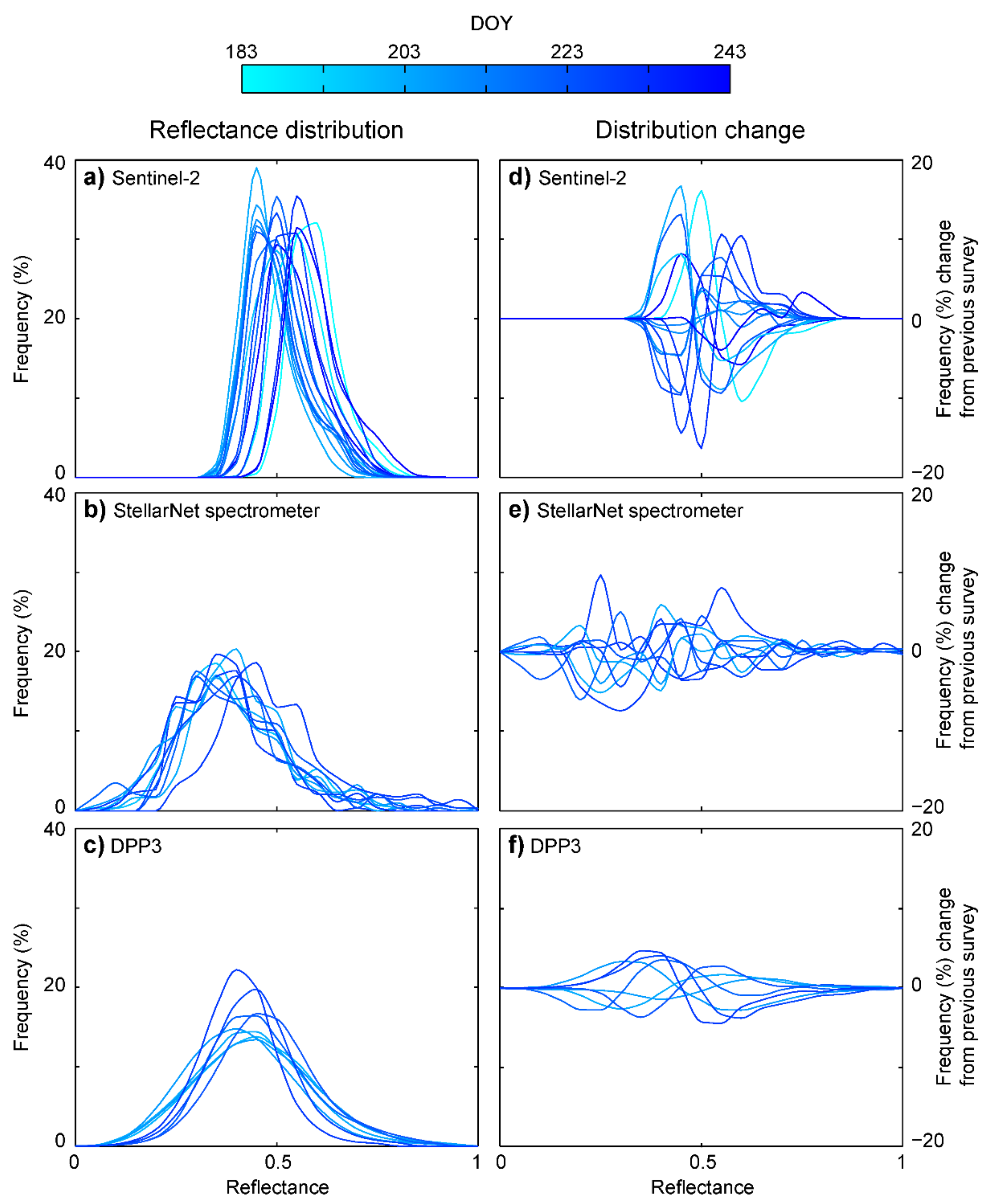
3.1. Bare-Ice Reflectance Variability

The 2016 melt season was darker than average [20], with MOD10A1 albedo persistently below the mean albedo recorded for the locality between 2000 and 2015 (Figure 2a). The long-term accumulated albedo proxy recorded at S6 suggested broadly stable surface reflectance typified the locality during the summer period: reflectance averaged ~0.47 (± 0.06) with intermittent, temporary decreases or increases (Figure 2c). These temporal variations qualitatively showed an association with the synoptic changes evidenced by periods of cloud cover which decreased SWin (e.g., DOY 199–202, 215, 222–224 and 229; Figure 2b). Bare ice persisted until DOY249, when snowfall increased reflectance at S6 to >0.7. Notwithstanding the uncertainty in representativeness of point measurements [46], the discrepancy between the HCRF reflectance approximations and true albedo [42,52,81], and the locational difference between our ROI and S6, the MOD10A1 albedo record for the 2016 bare-ice season (DOY180–250) correlates with the equivalent daily mean S6 reflectance time-series (r = 0.48, p < 0.001).
Significant correlations between the 10 pair-wise combinations of the MOD10A1, S6 reflectance, MOD09GQ and Sentinel-2 time-series (0.33 < r < 0.93, p < 0.01) highlighted the statistical similarity in the seasonal (JJA) pattern of local albedo and reflectance at the locality (Figure 2c–e). This overarching pattern was also observed in the ground-based SNBW and DPP3-derived reflectance data (Figure 2e), with means of 0.385 and 0.468, respectively. The cause of the lower SNBW average reflectance value is likely due to the sample locations for the SNBW measurements missing the brightest areas of the ice surface (see Figure 1b). Owing to the absence of concurrent measurements and a dearth of data pairs, retrieving correlations for these fine-scale observations with the satellite-derived time-series is not possible. Cloud cover can influence observed glacier surface albedo by up to 0.08 [23]; this likely results from the combined influence of factors, including the spectral attenuation of irradiance [82] on the heterogenous surface, and the changing optical properties of emergent, ablating ice [42]. During cloudy periods, typically the ratio of shortwave irradiance to turbulent energy fluxes decreases and this degrades and/or removes the more reflective, less consolidated and porous decimeter-scale surface ice layer that is created by the subsurface melting that is particularly associated with clear-sky conditions [26,83]. However, the DPP3 reflectance data collected on DOY224 and SNBW measurements on DOY 200 and 223 were consistent with similar records from clear-sky days. This suggests that, owing to the brevity and nature of the cloudy phases during our observation period, the effect of such influences was slight. With both reflectance datasets being generated from nadir downward-facing ratios and calibrated against the same white reference, these data are sufficiently representative.
As the spatial resolution of observations increases, the range of reflectance values also rises (Figure 2f). The coarser resolution of the Sentinel-2 product thus masks the finer resolution spatial variability through pixel scale spatial averaging. At the finest resolution of the DPP3 product, discrete and localized points of high or low reflectance are recorded. This variability is demonstrated in standard deviations of reflectance (σ; Figure 2g), particularly in the latter half of the period. Despite a high range, DPP3 shows a lowered σ, indicative of reduced variability around the mean, with a high degree of spatial autocorrelation [46]. The SNBW surveys show a smaller number of observations than the DPP3 spatial maps, and sample points at distances that are larger than the spatial autocorrelation, and so reveal more variability around the mean.
Changes in distribution between each measurement set are most clearly illustrated by the skewness (s) and kurtosis (k) (Figure 2h,i). The Sentinel-2, SNBW and DPP3 datasets all exhibit positive (right) skew, as previously reported for bare-ice using MODIS and Sentinel-2 data [26,45,47]. While the day-to-day variability in the distribution function for Sentinel-2 is masked as a result of the temporal resolution and the spatial averaging at the pixel scale, the higher spatial resolutions show that non-Gaussian distributions are persistent and that these distributions vary at the daily timescale. Such variability is suggestive of short-term changes and dynamics in the ice surface properties and characteristics.
Temporal variability is investigated further by examining spatial reflectance frequency distributions themselves (Figure 3a–c, refer also to Figure 1b). The spread of values depends on the dataset resolution: for example, Sentinel-2 shows narrower reflectance distributions compared to SNBW and DPP3, a result of spatial averaging within the pixel footprint, while the higher spatial resolution datasets better detail the range of reflectance seen over the heterogeneous bare-ice. With features, such as cryoconite holes, occupying ~8% of the surface area in the locality [84], the coarser resolution of Sentinel-2 eliminates observation of these discrete, ‘dark’ (<0.2) reflectance points and reduces the presence of tails within the distribution, with values exhibiting a closer fit around the mean. In contrast, the SNBW and DPP3 show a wider range, with spatial resolution able to capture the larger spread of reflectance values and, consequently, a lower mean. Over time, as shown by the distribution descriptors (Figure 2), the variations in the histogram form were not systematic. The change in distribution between each observation, for the three contrasting scale reflectance datasets, revealed changes of up to 20% (Figure 3d–f). This is indicative of a rapidly evolving and topographically complex bare-ice environment.
Our multi-scale observations support the previously identified need to examine sub-pixel variability in bare-ice surface reflectance in west Greenland [26,85], and to explore the relative precision of reflectance and/or albedo derived from platforms, particularly satellite platforms, at a range of scales. The discrepancies between in-situ HCRF, Sentinel-2 and MODIS products, as shown here, are unresolved yet well-known and often ascribed to differences in spatial aggregation and calibration of conversion methods [26,45,46,85]. While current methods often simplify the conversion of reflectance to albedo, at fine resolutions uncertainties in BRDFs, especially for lower reflectance surfaces common to heterogenous bare-ice environments typical of the ice sheet’s ablation zone, result in errors in albedo evaluation of up to 11% [52].
Our analysis shows that despite differences in sensor configuration, there are variations in the spatiotemporal patterns (Figure 3) of surface reflectance that can be resolved at each scale of measurement. This is critical, as it undermines the use of near-surface measurements, such as field spectroscopy and fixed-albedometers, as providing perfect benchmark satellite-validation tools [35]. Moreover, it also precludes the use of coarse-resolution satellite imagery to fully elucidate the processes operating across the ice surface that cause albedo to vary.

3.2. Reflectance Variability and Ablation

3.2.1. Spatial Variability

The ice melt (ablation) model [76] was used to examine the relevance of the spatial reflectance variability observed in this study. To begin, model runs employed a Gaussian reflectance distribution for variable mean albedo (Figure 4a), randomly assigned over the model domain (Figure 4b). Although linear conversions are feasible [74,86], in the absence of validated BRDF models at the necessary spatial resolution for impurity contaminated glacier ice, we use reflectance as a proxy for albedo (α). Comparison between model runs utilizing the arbitrary topography and a flat, unvaried surface yielded changes in the total melt of <0.5%; this result indicates that small-scale topography (slope and aspect variations) makes minimal difference to seasonal melt production. The mean reflectance varied while retaining a constant standard deviation (σ), skewness (s) and kurtosis (k), and revealed a linear response of surface melt to changes in albedo: a 0.01 change in bare-ice albedo increases or decreases melt by 2% (Figure 4e). As expected, retaining a constant mean (0.468, the average derived from the eight DPP3 surveys), and sequentially adjusting σ, s and k independently, resulted in negligible changes (<1%) in the melt production across the model runs, likely to be associated with the randomized population.
As we have shown, variability in the reflectance distribution across the ROI exhibits simultaneous changes to the mean, σ, s and k (Figure 2). To simulate these changes, a beta distribution was employed to describe α over the model domain. The standard beta probability density function, f(x), defined over the interval 0 to 1, is parameterized by two positive shape parameters (A and B > 0) and is well-suited to modelling the dynamic distributions of observations of a percentage variable, X (e.g., albedo measurements over space) [87]:
f x = x A 1 1 x B 1 β A , B 0     x     1 ;   A ,   B > 0
where x is a realization of X and β is the beta function. Here, again using the ice reflectance distribution obtained from the arbitrarily selected DPP3 survey on DOY205 as the ‘control’, we fitted a probability density function to the observed data, which defined parameters A and B as 2.108 and 2.583, respectively, (or A:B = 0.82; Figure 4c,d). As the beta distribution can also be defined by the sum of the shape parameters, we generated synthetic surface reflectance distributions for the model domain defined by A + B = 4.7; this provided positively and negatively skewed distributions with co-varied mean, σ, s and k (Figure 4c). The output from this second set of model runs highlighted a statistically similar inverse relationship between the mean reflectance and total melt (Figure 4e): 95% confidence intervals for the linear regressions showed significant similarity in the slope of the albedo-melt relationships. The mean daily variation of 0.025 exhibited in the MOD10A1 data series for 2016 implies that, for ablation controlled by albedo, daily changes in meltwater production were ±4.75%.
These simple simulations show that subtle changes in distribution of reflectance revealed by our nested examination of sub-MODIS-pixel variability in 2016 are not primary controls on melt production, at least at the scale of our ROI. It remains unclear as to whether coarser-resolution products (derived from MODIS or Sentinel-2) adequately and robustly represent pixel area mean reflectance through the assumed linear mixing models. Rather, our data suggest that for a given area, short-term (daily) changes in the areal mean reflectance may be an important control on melt production.

3.2.2. Temporal Variability

To assess the importance of temporal variation in areal mean reflectance of the bare-ice zone of western Greenland, we explored the efficacy of simulations of cumulative ablation against observed ablation (stake measurements) over the ROI by reporting the mean absolute error (MAE), the root mean squared error (RMSE) and the Nash-Sutcliffe Efficiency criterion (NSE: [88]) and Willmott Index of Agreement (d: [89]) which are predictive skill metrics commonly used in hydraulic modelling (Table 1). These metrics were also calculated for the average hourly melt rate each model predicted compared to that for the observed ablation measurements. Over the JJA period, characterized by clear skies and daily peak irradiance that was typically >500 Wm−2, the daily average air temperature remained above 0 °C throughout the summer (except for DOY182, 228, 229) until the autumn transition following DOY240 (Figure 5a). The variety of albedo parameterizations (Figure 5b) all performed similarly well in simulating cumulative ablation with goodness-of-fit metrics NSE and d > 0.9, and typical mean absolute errors of <0.10 m. The projections of cumulative bare-ice ablation of between 2.01 and 2.45 m w.e. (Figure 5c) fit well with the local long-term annual mean surface mass balance of −1.96 m w.e. at the IMAU S6 weather station [12], particularly in light of 2016 being a relatively moderate, unexceptional melt year [8].
The models that performed least well in predicting cumulative ablation across the goodness-of-fit metrics were the invariant fixed (αfix), minimum (αmin) and mean observed MOD10A1 (αMODmean) albedo parameterizations (Table 1); in contrast, all the models employing a dynamic albedo input yielded higher NSE and d indices, and lower MAE and RMSE (Table 1). Intermediate model performance was found for the linearly interpolated daily MOD10A1 series (αMODint), the lowest 10% MOD10A1 values (αmin5), and the composite product approximation (αMOD8dc). At the average hourly melt time-scale, despite modelled ablation using αfix resulting in high NSE and low MAE scores, across the model skill metrics, the dynamic albedo models consistently outperformed other formulations, and particularly the αmin5 and αMOD8dc parameterizations.
All the model runs exhibited an underestimation of melt between DOY199 and 217 (Figure 5d), when reflectance values were low (Figure 2). With seasonal minimum albedo typically reached ~36 days after bare-ice onset [90], we speculate that this underestimation of melt is a function of ice algae: discrete algal blooms not only darken the ice surface over length-scales below that of the resolution of satellite observation, but also exhibit non-linear growth following a brief lag phase after the onset of bare-ice conditions [25,26,27,44]. These biological early melt season processes may not be fully captured by either satellite products or air temperature-derived estimations of albedo. Following DOY218, all of the model variants fall within the range of observed ablation measurements, which also illustrate the cumulative uncertainties associated with the ground-based measurements themselves. Examination of our modelled ablation during the observation period highlights how the temporally dynamic α simulations performed almost identically (Figure 5d): all yielding RMSEs < 0.013 m w.e. and mirroring the αMODint output. These latter models all tracked the ROI’s median ablation well, and show that the use of poorly defined, invariant albedo values can result in over- or under-estimation of cumulative summer ablation by ±11%.

4. Discussion

Our multi-scale analysis reveals a spatial and temporal heterogeneity of bare-ice reflectance in the western section of the Greenland Ice Sheet. The daily MODIS MOD10A1 albedo record for the pixel containing our study site during the 2016 summer JJA melt season exhibited a decreasing trend followed by an increase, over a range of 0.26, superimposed with day-to-day variation up to 0.09. Even excluding the end of summer period from DOY240, the seasonal bare-ice albedo variation of 0.16 exceeds the 0.11 reported for bare-ice across the ice sheet [90]; late season increases in surface reflectance is not solely a result of late season snowfall accumulation [90], but rather can also arise independently from the formation of ice lids and/or freeze-up of cryoconite holes [34] and initial autumn superimposed ice formation [13,33]. The daily variability, however, is comparable to or below the uncertainties reported from assessments of the MOD10A1 product of between 0.03 to 0.1 [14,45,46,91], with the greater magnitudes of uncertainty likely in the JJA period owing to bare-ice heterogeneity [35]. The MOD10A1 product failed to resolve albedo increase [26], despite Sentinel-2 and fine-scale multi-spectral measurements showing substantial increases in clean ice over the pixel scale. Consequently, confidence in the short-term variations in the MOD10A1 record may be questioned. Nonetheless, similar seasonal and marked daily-to-synoptic scale variations in the daily and composite MOD09 reflectance products and the weekly Sentinel-2 observations for the bare-ice period during the melt season are observed.
Mean summer reflectance in the 0.25 km2 ROI study site from Sentinel-2 showed the same seasonal cycle as that observed in the MOD10A1 time series, albeit over a smaller reflectance range (~0.13). However, Sentinel-2′s coarse temporal resolution precludes identification of shorter-term variability and surface reflectance value tend towards the higher end of in-situ measurements (e.g., our DPP3 and SNBW data, see Figure 3), and darker and brighter surfaces and over- and under-estimated, respectively [92]. This is due to areal averaging of sub-pixel (<10 m) scale heterogeneities. Spatial aggregation of mean surface characteristics at both the MODIS (250 or 500 m) and Sentinel-2 (10 m) pixel scale is enhanced due to some impurities (e.g., cryoconite holes that are less than 1 m in diameter; Figure 1b) being obscured from non-zenith illumination and non-nadir observation angles [35,45,46] and spatial changes occurring at sub-pixel length scales [25,26].
Despite showing similar, relatively small (<0.13) daily to multi-day changes in mean reflectance, as observed by Sentinel-2, our finer scale data displayed increased standard deviation (σ > 0.1) and range (>0.95) in the reflectance distribution. Such resolution-dependent distribution has been reported elsewhere [52]. Cloud cover is known to adjust retrieved reflectance derived from ground- and UAV-based measurement platforms owing to changes in the downwelling and upwelling spectral energy distributions [85,93]. However, only three days of our fine-resolution observations were influenced by cloud cover, and deviations in reflectance distribution were not particularly marked; changes in spatial mean reflectance were characteristically less than the maximum of 0.08 identified for cloud-effects on HCRF broadband reflectance for Greenland ice types [23]. These findings suggest that processes causing variations in the apparent optical properties of bare-ice at daily timescales under clear sky conditions may have a similar magnitude impact on surface albedo as changes in cloud cover. Therefore, we argue that the reflectance records presented here demonstrate a seasonal and daily variability in bare-ice reflectance distribution and, by inference, a spatiotemporal heterogeneity in the albedo of the bare-ice surface, as implied by the MOD10A1 data record.
The processes underlying the dynamics in the optical characteristics of the bare-ice environment of our ROI are expressed in not only the mean surface reflectance but its changing distributions. Such seasonal and synoptic transitions in reflectance and albedo distributions have previously been reported in western Greenland [26,47]. At the start of the bare-ice phase, higher reflectance (>0.6) surfaces, such as residual seasonal snow and superimposed ice, result in either bimodal or negatively skewed unimodal reflectance distributions [45,47]. However, our fine-resolution data does not capture these early season conditions, and despite the elevated mean reflectance (DOY183–193) shown by Sentinel-2, its spatial resolution and sampling bias [92] likely masks the true expression of the reflectance distributions. Once early summer season bright surfaces are eliminated, with increased exposure of darker bare-ice, and associated impurities, meltwater and ice algal growth, the mean reflectance decreases and reflectance distributions tend to be those with a positive skew with variable kurtosis, as evident in our multi-scale datasets. Subsequently, as ice ablation is reduced later in the season, mean reflectance increases and skewness declines with a clear trend toward negative skew (Figure 2h); we acknowledge, however, that due to the synoptic event evident for DOY236–243 and the duration of our fine-resolution observations, our datasets do not fully capture the freeze-up of the bare-ice surface.
At the scale of a MODIS pixel, skew in reflectance distribution may result in a 2% increase in hourly surface melt predictions [26]. Based on our model of ablation utilizing a beta distribution to simulate a skewed surface albedo distribution, we demonstrate that the nature of the albedo distribution skew is not itself critical for simulating melt at daily to seasonal timescales if the areal mean surface albedo is accurately characterized. Recognition of the temporal evolution of the areal mean albedo of the bare-ice surface is, instead, crucial. Approaches utilizing temporally (and spatially) constant representations of bare-ice albedo will be subject to greater uncertainties: arbitrary bare-ice albedo or an albedo defined by the lowest observed value(s) for a location may, respectively, under- or over-predict seasonal ablation by ~10%. Certainly, for Greenland’s dark zone and other marginal areas, assumptions that bare-ice albedo lies between 0.5 and 0.55 [54], which is closer to the bare-ice onset of 0.565 [90], will underestimate ice melt. Similarly, use of satellite-derived albedo minima will overestimate melt through lacking recognition of the seasonal changes in the optical properties of the ice surface.
Our ablation model sensitivity analysis study shows how the use of an albedo parameterization that portrays short-term (daily) temporal variability, rather than fixed values, results in improved ablation estimates. Here, ablation model performance at seasonal and daily (or average hourly) time-scales was improved whether accounting for fine scale temporal variability by using a mean albedo calculated from linearly interpolated daily time-series of the MOD10A1 record [58] or by employing more sophisticated periodically evolving [57], time-dependent, or physically based parameterizations. Consequently, our results support the use of melt-dependent parameterizations [39], as employed within the Modèle Atmosphérique Régionale (MAR) [18,94]; although in its current form, with α limited to >0.4, MAR likely underestimates ablation, particularly in the darker regions of the Greenland Ice Sheet. We therefore argue that exploration, development and testing of cyclical or physically based bare-ice albedo dynamics at moderate to high temporal resolution are required for further forecasting and sensitivity studies.
Irrespective of the data source uncertainties in observing true bare-ice albedo, this study emphasizes the need to account for the short-term spatial variation in the optical properties of the bare-ice surface in modelling ice ablation. Specifically, there is a need to constrain the representativeness and accuracy of the spatial mean albedo at numerical model grid resolutions. While dynamic non-Gaussian reflectance distributions, primarily arising from ice surface processes, are themselves not an important consideration for ablation, at least at daily timescales, definition of representative spatial mean reflectance observations, and variability therein, is essential for accurate predictions of bare-ice melt at daily to seasonal timescales. To achieve this, it is critical that the inherent surface variability induced by the biologically active, ablating ice interface is recognized. With some regions in Greenland recently experiencing increased clear-sky conditions [3,4], high-pressure blocking [95,96], rising air temperatures [2] and increasing bare-ice areas [8,9], adequately characterizing bare-ice albedo, and its spatiotemporal evolution, is critical to improving projections of the ice sheet’s surface mass balance.

5. Conclusions

Despite its critical role in amplifying Greenland’s ice ablation, bare-ice albedo remains poorly characterized and parameterized in numerical models. Here, we demonstrate substantial spatial and temporal variability in the reflectance of the bare-ice environment using a multi-scale analysis that uniquely draws together and compares finer-resolution ground-based spectrometry, UAV- and Sentinel-2 derived reflectance observations and the coarse resolution MODIS reflectance and albedo products. Our analysis highlights daily-to-seasonal synoptic variability in bare-ice reflectance, evident in both the spatially averaged reflectance for our 1300 m2 study area along with the actual reflectance distributions measured in-situ with a field-spectrometer. At the highest spatial resolution, varying but consistently positive skewed reflectance distributions were observed throughout the 2016 peak melt season. Modelling bare-ice melt with these reflectance distributions described using a beta function yields no significant difference compared to a Gaussian distribution, but highlights the importance of accurately describing the areal mean albedo. Further assessment exploring the temporal variability in bare-ice albedo emphasizes the critical importance of parameterizations at daily-to-synoptic resolution, with inappropriate schemes yielding large errors in seasonal ablation of up to 11%. Given that summer high-pressure, clear-sky blocking conditions have been increasing in the last 30 years, with concomitant air temperature warming and expansion of ice sheet ablation areas, we argue that future research efforts must provide robust albedo evaluations for heterogenous bare-ice across the range of available observational platform scales, and further refine evolving bare-ice albedo parameterizations using temporally and physically based descriptors.

Author Contributions

Conceptualization, T.D.L.I.-F., P.B. and J.M.C.; Methodology, T.D.L.I.-F., P.B., A.J.H. (Andy J. Hardy), J.M.C., K.N. and M.H.; Investigation and Data Acquisition, T.D.L.I.-F., P.B., J.M.C., A.J.H. (Andy J. Hardy), J.B.M., J.N., O.R., A.J.T., M.T. and C.J.W.; Formal Analysis, T.D.L.I.-F., P.B., O.R., K.N., M.H. and A.H.; Data Curation, T.D.L.I.-F., P.B., A.J.H. (Andy J. Hardy), J.M.C. and O.R.; Writing—Original Draft Preparation, T.D.L.I.-F., P.B., J.M.C., J.C.R. and A.H.; Writing—Review & Editing, A.H., N.E.B., J.M.C., J.C.R., E.H., A.J.H. (Andrew J. Hodson), T.O.H., A.J.T. and C.J.W.; Visualization, T.D.L.I.-F., P.B. and O.R.; Funding Acquisition, M.T., A.J.H. (Andrew J. Hodson), E.H. and T.D.L.I.-F. All authors have read and agreed to the published version of the manuscript.

Funding

This research was funded by NERC’s Large Grant ‘Black and Bloom’ (NE/M020991/1, NE/M021025/1, NE/M021084/1 and NE/M020770/1) supporting T.D.L.I.-F., J.M.C., E.H., A.J.H. (Andrew J. Hodson), J.B.M., J.N., A.J.T., M.T., C.J.W.; T.D.L.I.-F. acknowledges Leverhulme Trust Research Fellowship RF-2018-584/4; K.N. acknowledges SNSF Mobility Fellowship Grant (P2FRP2/174888); A.H. acknowledges a research professorship from the Research Council of Norway through its Centres of Excellence scheme (Grant 223259) and an Academy of Finland visiting fellowship to the University of Oulu. J.N. was supported by the NASA MEaSUREs ITS_LIVE project, the NASA Cryospheric Sciences program the Jet Propulsion Laboratory, California Institute of Technology, through an agreement with the National Aeronautics and Space Administration.

Institutional Review Board Statement

Not applicable.

Informed Consent Statement

Not applicable.

Data Availability Statement

The data presented in this study are available on the Zenodo repository at https://doi.org/10.5281/zenodo.5735626.

Acknowledgments

Constructive comments from three anonymous reviewers are acknowledged for improving the clarity of the paper. Morgan Jones, Neil Glasser, Oliver Bartlett and Hywel Griffiths are thanked for commenting on earlier drafts.

Conflicts of Interest

The authors declare no conflict of interest.

References

  1. Trusel, L.D.; Das, S.B.; Osman, M.B.; Evans, M.J.; Smith, B.; Fettweis, X.; McConnell, J.R.; Noel, B.P.Y.; van den Broeke, M.R. Nonlinear rise in Greenland runoff in response to post-industrial Arctic warming. Nature 2018, 564, 104–108. [Google Scholar] [CrossRef]
  2. Hanna, E.; Cappelen, J.; Fettweis, X.; Mernild, S.H.; Mote, T.L.; Mottram, R.; Steffen, K.; Ballinger, T.J.; Hall, R. Greenland surface air temperature changes from 1981 to 2019 and implications for ice-sheet melt and mass-balance change. Int. J. Climatol. 2021, 41, E1336–E1352. [Google Scholar] [CrossRef]
  3. Hofer, S.; Tedstone, A.J.; Fettweis, X.; Bamber, J.L. Decreasing cloud cover drives the recent mass loss on the Greenland Ice Sheet. Sci. Adv. 2017, 3, e1700584. [Google Scholar] [CrossRef] [Green Version]
  4. Hanna, E.; Cropper, T.E.; Hall, R.J.; Cappelen, J. Greenland Blocking Index 1851–2015: A regional climate change signal. Int. J. Climatol. 2016, 36, 4847–4861. [Google Scholar] [CrossRef] [Green Version]
  5. Doyle, S.H.; Hubbard, A.; van de Wal, R.S.W.; Box, J.E.; van As, D.; Scharrer, K.; Meierbachtol, T.W.; Smeets, P.C.J.P.; Harper, J.T.; Johansson, E.; et al. Amplified melt and flow of the Greenland ice sheet driven by late-summer cyclonic rainfall. Nat. Geosci. 2015, 8, 647–653. [Google Scholar] [CrossRef]
  6. Oltmanns, M.; Straneo, F.; Tedesco, M. Increased Greenland melt triggered by large-scale, year-round cyclonic moisture intrusions. Cryosphere 2019, 13, 815–825. [Google Scholar] [CrossRef] [Green Version]
  7. Fettweis, X.; Tedesco, M.; van den Broeke, M.; Ettema, J. Melting trends over the Greenland ice sheet (1958–2009) from spaceborne microwave data and regional climate models. Cryosphere 2011, 5, 359–375. [Google Scholar] [CrossRef] [Green Version]
  8. Noel, B.; van de Berg, W.J.; Lhermitte, S.; van den Broeke, M.R. Rapid ablation zone expansion amplifies north Greenland mass loss. Sci. Adv. 2019, 5, eaaw0123. [Google Scholar] [CrossRef] [Green Version]
  9. Ryan, J.C.; Smith, L.C.; van As, D.; Cooley, S.W.; Cooper, M.G.; Pitcher, L.H.; Hubbard, A. Greenland Ice Sheet surface melt amplified by snowline migration and bare ice exposure. Sci. Adv. 2019, 5, eaav3738. [Google Scholar] [CrossRef] [Green Version]
  10. Shepherd, A.; Ivins, E.; Rignot, E.; Smith, B.; van den Broeke, M.; Velicogna, I.; Whitehouse, P.; Briggs, K.; Joughin, I.; Krinner, G.; et al. Mass balance of the Greenland Ice Sheet from 1992 to 2018. Nature 2020, 579, 233–239. [Google Scholar] [CrossRef]
  11. Steger, C.R.; Reijmer, C.H.; van den Broeke, M.R. The modelled liquid water balance of the Greenland Ice Sheet. Cryosphere 2017, 11, 2507–2526. [Google Scholar] [CrossRef] [Green Version]
  12. Munneke, P.K.; Smeets, C.J.P.P.; Reijmer, C.H.; Oerlemans, J.; van de Wal, R.S.W.; van den Broeke, M.R. The K-transect on the western Greenland Ice Sheet: Surface energy balance (2003–2016). Arct. Antarct. Alp. Res. 2018, 50, e1420952. [Google Scholar] [CrossRef] [Green Version]
  13. Van den Broeke, M.; Smeets, P.; Ettema, J.; van der Veen, C.; van de Wal, R.; Oerlemans, J. Partitioning of melt energy and meltwater fluxes in the ablation zone of the west Greenland ice sheet. Cryosphere 2008, 2, 179–189. [Google Scholar] [CrossRef] [Green Version]
  14. Box, J.E.; Fettweis, X.; Stroeve, J.C.; Tedesco, M.; Hall, D.K.; Steffen, K. Greenland ice sheet albedo feedback: Thermodynamics and atmospheric drivers. Cryosphere 2012, 6, 821–839. [Google Scholar] [CrossRef] [Green Version]
  15. Helsen, M.M.; van de Wal, R.S.W.; Reerink, T.J.; Bintanja, R.; Madsen, M.S.; Yang, S.T.; Li, Q.; Zhang, Q. On the importance of the albedo parameterization for the mass balance of the Greenland ice sheet in EC-Earth. Cryosphere 2017, 11, 1949–1965. [Google Scholar] [CrossRef] [Green Version]
  16. He, T.; Liang, S.L.; Yu, Y.Y.; Wang, D.D.; Gao, F.; Liu, Q. Greenland surface albedo changes in July 1981–2012 from satellite observations. Environ. Res. Lett. 2013, 8, 044043. [Google Scholar] [CrossRef]
  17. Riihela, A.; King, M.D.; Anttila, K. The surface albedo of the Greenland Ice Sheet between 1982 and 2015 from the CLARA-A2 dataset and its relationship to the ice sheet’s surface mass balance. Cryosphere 2019, 13, 2597–2614. [Google Scholar] [CrossRef] [Green Version]
  18. Tedesco, M.; Doherty, S.; Fettweis, X.; Alexander, P.; Jeyaratnam, J.; Stroeve, J. The darkening of the Greenland ice sheet: Trends, drivers, and projections (1981–2100). Cryosphere 2016, 10, 477–496. [Google Scholar] [CrossRef] [Green Version]
  19. Shimada, R.; Takeuchi, N.; Aoki, T. Inter-annual and geographical variations in the extent of bare ice and dark ice on the Greenland Ice Sheet derived from MODIS satellite images. Front. Earth Sci. 2016, 4, 43. [Google Scholar] [CrossRef] [Green Version]
  20. Tedstone, A.J.; Bamber, J.L.; Cook, J.M.; Williamson, C.J.; Fettweis, X.; Hodson, A.J.; Tranter, M. Dark ice dynamics of the south-west Greenland Ice Sheet. Cryosphere 2017, 11, 2491–2506. [Google Scholar] [CrossRef] [Green Version]
  21. Van den Broeke, M.; Box, J.; Fettweis, X.; Hanna, E.; Noel, B.; Tedesco, M.; van As, D.; van de Berg, W.J.; van Kampenhout, L. Greenland Ice Sheet surface mass loss: Recent developments in observation and modeling. Curr. Clim. Change Rep. 2017, 3, 345–356. [Google Scholar] [CrossRef] [Green Version]
  22. Van de Berg, W.J.; van Meijgaard, E.; van Ulft, L.H. The added value of high resolution in estimating the surface mass balance in southern Greenland. Cryosphere 2020, 14, 1809–1827. [Google Scholar] [CrossRef]
  23. Boggild, C.E.; Brandt, R.E.; Brown, K.J.; Warren, S.G. The ablation zone in northeast Greenland: Ice types, albedos and impurities. J. Glaciol. 2010, 56, 101–113. [Google Scholar] [CrossRef] [Green Version]
  24. Goelles, T.; Boggild, C.E. Albedo reduction of ice caused by dust and black carbon accumulation: A model applied to the K-transect, West Greenland. J. Glaciol. 2017, 63, 1063–1076. [Google Scholar] [CrossRef] [Green Version]
  25. Stibal, M.; Box, J.E.; Cameron, K.A.; Langen, P.L.; Yallop, M.L.; Mottram, R.H.; Khan, A.L.; Molotch, N.P.; Chrismas, N.A.M.; Quaglia, F.C.; et al. Algae drive enhanced darkening of bare ice on the Greenland Ice Sheet. Geophys. Res. Lett. 2017, 44, 11463–11471. [Google Scholar] [CrossRef]
  26. Tedstone, A.J.; Cook, J.M.; Williamson, C.J.; Hofer, S.; McCutcheon, J.; Irvine-Fynn, T.; Gribbin, T.; Tranter, M. Algal growth and weathering crust state drive variability in western Greenland Ice Sheet ice albedo. Cryosphere 2020, 14, 521–538. [Google Scholar] [CrossRef] [Green Version]
  27. Williamson, C.J.; Anesio, A.M.; Cook, J.; Tedstone, A.; Poniecka, E.; Holland, A.; Fagan, D.; Tranter, M.; Yallop, M.L. Ice algal bloom development on the surface of the Greenland Ice Sheet. FEMS Microbiol. Ecol. 2018, 94, fiy025. [Google Scholar] [CrossRef] [PubMed]
  28. Jones, C.; Ryan, J.; Holt, T.; Hubbard, A. Structural glaciology of Isunguata Sermia, West Greenland. J. Maps 2018, 14, 517–527. [Google Scholar] [CrossRef] [Green Version]
  29. Wientjes, I.G.M.; van de Wal, R.S.W.; Schwikowski, M.; Zapf, A.; Fahrni, S.; Wacker, L. Carbonaceous particles reveal that Late Holocene dust causes the dark region in the western ablation zone of the Greenland ice sheet. J. Glaciol. 2012, 58, 787–794. [Google Scholar] [CrossRef] [Green Version]
  30. Ryan, J.C.; Hubbard, A.; Stibal, M.; Irvine-Fynn, T.D.; Cook, J.; Smith, L.C.; Cameron, K.; Box, J. Dark zone of the Greenland Ice Sheet controlled by distributed biologically-active impurities. Nat. Commun. 2018, 9, 1065. [Google Scholar] [CrossRef] [PubMed] [Green Version]
  31. Williamson, C.J.; Cook, J.; Tedstone, A.; Yallop, M.; McCutcheon, J.; Poniecka, E.; Campbell, D.; Irvine-Fynn, T.; McQuaid, J.; Tranter, M.; et al. Algal photophysiology drives darkening and melt of the Greenland Ice Sheet. Proc. Natl. Acad. Sci. USA 2020, 117, 5694–5705. [Google Scholar] [CrossRef] [PubMed] [Green Version]
  32. Janssens, I.; Huybrechts, P. The treatment of meltwater retention in mass-balance parameterizations of the Greenland ice sheet. Ann. Glaciol. 2000, 31, 133–140. [Google Scholar] [CrossRef] [Green Version]
  33. Pfeffer, W.T.; Meier, M.F.; Illangasekare, T.H. Retention of Greenland runoff by refreezing: Implications for projected future sea-level change. J. Geophys. Res. Oceans 1991, 96, 22117–22124. [Google Scholar] [CrossRef]
  34. Hodson, A.; Boggild, C.; Hanna, E.; Huybrechts, P.; Langford, H.; Cameron, K.; Houldsworth, A. The cryoconite ecosystem on the Greenland ice sheet. Ann. Glaciol. 2010, 51, 123–129. [Google Scholar] [CrossRef] [Green Version]
  35. Ryan, J.C.; Hubbard, A.; Box, J.E.; Brough, S.; Cameron, K.; Cook, J.M.; Cooper, M.; Doyle, S.H.; Edwards, A.; Holt, T.; et al. Derivation of High Spatial Resolution Albedo from UAV Digital Imagery: Application over the Greenland Ice Sheet. Front. Earth Sci. 2017, 5, 40. [Google Scholar] [CrossRef] [Green Version]
  36. Wientjes, I.G.M.; Van de Wal, R.S.W.; Reichart, G.J.; Sluijs, A.; Oerlemans, J. Dust from the dark region in the western ablation zone of the Greenland ice sheet. Cryosphere 2011, 5, 589–601. [Google Scholar] [CrossRef] [Green Version]
  37. Cooper, M.G.; Smith, L.C.; Rennermalm, A.K.; Miege, C.; Pitcher, L.H.; Ryan, J.C.; Yang, K.; Cooley, S. Meltwater storage in low-density near-surface bare ice in the Greenland ice sheet ablation zone. Cryosphere 2018, 12, 955–970. [Google Scholar] [CrossRef] [Green Version]
  38. Greuell, W. Melt-water accumulation on the surface of the Greenland ice sheet: Effect on albedo and mass balance. Geogr. Ann. A 2000, 82, 489–498. [Google Scholar] [CrossRef]
  39. Zuo, Z.; Oerlemans, J. Modelling albedo and specific balance of the Greenland ice sheet: Calculations for the Sondre Stromfjord transect. J. Glaciol. 1996, 42, 305–317. [Google Scholar] [CrossRef]
  40. Yang, K.; Smith, L.C.; Cooper, M.G.; Pitcher, L.H.; van As, D.; Lu, Y.; Lu, X.; Li, M.C. Seasonal evolution of supraglacial lakes and rivers on the southwest Greenland Ice Sheet. J. Glaciol. 2021, 67, 592–602. [Google Scholar] [CrossRef]
  41. Chandler, D.M.; Alcock, J.D.; Wadham, J.L.; Mackie, S.L.; Telling, J. Seasonal changes of ice surface characteristics and productivity in the ablation zone of the Greenland Ice Sheet. Cryosphere 2015, 9, 487–504. [Google Scholar] [CrossRef] [Green Version]
  42. Cook, J.M.; Hodson, A.J.; Gardner, A.S.; Flanner, M.; Tedstone, A.J.; Williamson, C.; Irvine-Fynn, T.D.L.; Nilsson, J.; Bryant, R.; Tranter, M. Quantifying bioalbedo: A new physically based model and discussion of empirical methods for characterising biological influence on ice and snow albedo. Cryosphere 2017, 11, 2611–2632. [Google Scholar] [CrossRef] [Green Version]
  43. Takeuchi, N.; Sakaki, R.; Uetake, J.; Nagatsuka, N.; Shimada, R.; Niwano, M.; Aoki, T. Temporal variations of cryoconite holes and cryoconite coverage on the ablation ice surface of Qaanaaq Glacier in northwest Greenland. Ann. Glaciol. 2018, 59, 21–30. [Google Scholar] [CrossRef] [Green Version]
  44. Cook, J.M.; Tedstone, A.J.; Williamson, C.; McCutcheon, J.; Hodson, A.J.; Dayal, A.; Skiles, M.; Hofer, S.; Bryant, R.; McAree, O.; et al. Glacier algae accelerate melt rates on the south-western Greenland Ice Sheet. Cryosphere 2020, 14, 309–330. [Google Scholar] [CrossRef] [Green Version]
  45. Moustafa, S.E.; Rennermalm, A.K.; Roman, M.O.; Wang, Z.S.; Schaaf, C.B.; Smith, L.C.; Koenig, L.S.; Erb, A. Evaluation of satellite remote sensing albedo retrievals over the ablation area of the southwestern Greenland ice sheet. Remote Sens. Environ. 2017, 198, 115–125. [Google Scholar] [CrossRef]
  46. Ryan, J.C.; Hubbard, A.; Irvine-Fynn, T.D.; Doyle, S.H.; Cook, J.M.; Stibal, M.; Box, J.E. How robust are in situ observations for validating satellite-derived albedo over the dark zone of the Greenland Ice Sheet? Geophys. Res. Lett. 2017, 44, 6218–6225. [Google Scholar] [CrossRef] [Green Version]
  47. Moustafa, S.E.; Rennermalm, A.K.; Smith, L.C.; Miller, M.A.; Mioduszewski, J.R.; Koenig, L.S.; Hom, M.G.; Shuman, C.A. Multi-modal albedo distributions in the ablation area of the southwestern Greenland Ice Sheet. Cryosphere 2015, 9, 905–923. [Google Scholar] [CrossRef] [Green Version]
  48. Cathles, L.M.; Abbot, D.S.; Bassis, J.N.; MacAyeal, D.R. Modeling surface-roughness/solar-ablation feedback: Application to small-scale surface channels and crevasses of the Greenland ice sheet. Ann. Glaciol. 2011, 52, 99–108. [Google Scholar] [CrossRef] [Green Version]
  49. Nolin, A.W.; Payne, M.C. Classification of glacier zones in western Greenland using albedo and surface roughness from the Multi-angle Imaging SpectroRadiometer (MISR). Remote Sens. Environ. 2007, 107, 264–275. [Google Scholar] [CrossRef]
  50. Knap, W.H.; Oerlemans, J. The surface albedo of the Greenland ice sheet: Satellite-derived and in situ measurements in the Sondre Stromfjord area during the 1991 melt season. J. Glaciol. 1996, 42, 364–374. [Google Scholar] [CrossRef] [Green Version]
  51. Greuell, W.; Reijmer, C.H.; Oerlemans, J. Narrowband-to-broadband albedo conversion for glacier ice and snow based on aircraft and near-surface measurements. Remote Sens. Environ. 2002, 82, 48–63. [Google Scholar] [CrossRef]
  52. Naegeli, K.; Damm, A.; Huss, M.; Wulf, H.; Schaepman, M.; Hoelzle, M. Cross-comparison of albedo products for glacier surfaces derived from airborne and satellite (Sentinel-2 and Landsat 8) optical data. Remote Sens. 2017, 9, 110. [Google Scholar] [CrossRef] [Green Version]
  53. Alexander, P.M.; LeGrande, A.N.; Fischer, E.; Tedesco, M.; Fettweis, X.; Kelley, M.; Nowicki, S.M.J.; Schmidt, G.A. Simulated Greenland surface mass balance in the GISS Model E2 GCM: Role of the ice sheet surface. J. Geophys. Res. Earth 2019, 124, 750–765. [Google Scholar] [CrossRef]
  54. Bougamont, M.; Bamber, J.L. A surface mass balance model for the Greenland ice sheet. J. Geophys. Res. Earth 2005, 110, F04018. [Google Scholar] [CrossRef]
  55. Rae, J.G.L.; Aoalgeirsdottir, G.; Edwards, T.L.; Fettweis, X.; Gregory, J.M.; Hewitt, H.T.; Lowe, J.A.; Lucas-Picher, P.; Mottram, R.H.; Payne, A.J.; et al. Greenland ice sheet surface mass balance: Evaluating simulations and making projections with regional climate models. Cryosphere 2012, 6, 1275–1294. [Google Scholar] [CrossRef] [Green Version]
  56. Noel, B.; van de Berg, W.J.; Machguth, H.; Lhermitte, S.; Howat, I.; Fettweis, X.; van den Broeke, M.R. A daily, 1 km resolution data set of downscaled Greenland ice sheet surface mass balance (1958–2015). Cryosphere 2016, 10, 2361–2377. [Google Scholar] [CrossRef] [Green Version]
  57. Navari, M.; Margulis, S.A.; Tedesco, M.; Fettweis, X.; Alexander, P.M. Improving Greenland surface mass balance estimates through the assimilation of MODIS albedo: A case study along the K-Transect. Geophys. Res. Lett. 2018, 45, 6549–6556. [Google Scholar] [CrossRef]
  58. Williamson, S.N.; Copland, L.; Thomson, L.; Burgess, D. Comparing simple albedo scaling methods for estimating Arctic glacier mass balance. Remote Sens. Environ. 2020, 246, 111858. [Google Scholar] [CrossRef]
  59. Dumont, M.; Gardelle, J.; Sirguey, P.; Guillot, A.; Six, D.; Rabatel, A.; Arnaud, Y. Linking glacier annual mass balance and glacier albedo retrieved from MODIS data. Cryosphere 2012, 6, 1527–1539. [Google Scholar] [CrossRef] [Green Version]
  60. Colgan, W.; Box, J.E.; Fausto, R.S.; van As, D.; Barletta, V.R.; Forsberg, R. Surface albedo as a proxy for the mass balance of Greenland’s terrestrial ice. Geol. Surv. Den. Greenl. 2014, 31, 91–94. [Google Scholar] [CrossRef] [Green Version]
  61. Wilton, D.J.; Jowett, A.; Hanna, E.; Bigg, G.R.; van den Broeke, M.R.; Fettweis, X.; Huybrechts, P. High resolution (1 km) positive degree-day modelling of Greenland ice sheet surface mass balance, 1870–2012 using reanalysis data. J. Glaciol. 2017, 63, 176–193. [Google Scholar] [CrossRef] [Green Version]
  62. Hubbard, B.; Glasser, N.F. Field Techniques in Glaciology and Glacial Geomorphology; John Wiley & Sons: Chichester, UK, 2005. [Google Scholar]
  63. Smeets, P.C.J.P.; Munneke, P.K.; van As, D.; van den Broeke, M.R.; Boot, W.; Oerlemans, H.; Snellen, H.; Reijmer, C.H.; van de Wal, R.S.W. The K-transect in west Greenland: Automatic weather station data (1993–2016). Arct. Antarct. Alp. Res. 2018, 50, e1420954. [Google Scholar] [CrossRef] [Green Version]
  64. Hall, D.K.; Riggs, G.A. MODIS/Terra Snow Cover Daily L3 Global 0.05 Deg CMG, Version 6. 2019. Available online: https://nsidc.org/data/MOD10A1/versions/6 (accessed on 9 March 2021).
  65. Casey, K.A.; Polashenski, C.M.; Chen, J.; Tedesco, M. Impact of MODIS sensor calibration updates on Greenland Ice Sheet surface reflectance and albedo trends. Cryosphere 2017, 11, 1781–1795. [Google Scholar] [CrossRef] [Green Version]
  66. Vermote, E.F.; ElSaleous, N.; Justice, C.O.; Kaufman, Y.J.; Privette, J.L.; Remer, L.; Roger, J.C.; Tanre, D. Atmospheric correction of visible to middle-infrared EOS-MODIS data over land surfaces: Background, operational algorithm and validation. J. Geophys. Res. Atmos. 1997, 102, 17131–17141. [Google Scholar] [CrossRef] [Green Version]
  67. Bunting, P.; Clewley, D. Atmospheric and Radiometric Correction of Satellite Imagery (ARCSI). 2018. Available online: https://remotesensing.info/arcsi/ (accessed on 1 September 2021).
  68. Cutler, P.M.; Munro, D.S. Visible and near-infrared reflectivity during the ablation period on Peyto Glacier, Alberta, Canada. J. Glaciol. 1996, 42, 333–340. [Google Scholar] [CrossRef] [Green Version]
  69. Schaepman-Strub, G.; Schaepman, M.E.; Painter, T.H.; Dangel, S.; Martonchik, J.V. Reflectance quantities in optical remote sensing-definitions and case studies. Remote Sens. Environ. 2006, 103, 27–42. [Google Scholar] [CrossRef]
  70. Ryan, J.C.; Hubbard, A.L.; Box, J.E.; Todd, J.; Christoffersen, P.; Carr, J.R.; Holt, T.O.; Snooke, N. UAV photogrammetry and structure from motion to assess calving dynamics at Store Glacier, a large outlet draining the Greenland ice sheet. Cryosphere 2015, 9, 1–11. [Google Scholar] [CrossRef] [Green Version]
  71. Moran, M.S.; Bryant, R.; Thome, K.; Ni, W.; Nouvellon, Y.; Gonzalez-Dugo, M.P.; Qi, J. A refined empirical line approach for reflectance factor retrieval from Landsat-5 TM and Landsat-7 ETM+. Remote Sens. Environ. 2001, 78, 71–82. [Google Scholar] [CrossRef]
  72. Smith, G.M.; Milton, E.J. The use of the empirical line method to calibrate remotely sensed data to reflectance. Int. J. Remote Sens. 1999, 20, 2653–2662. [Google Scholar] [CrossRef]
  73. Boggs, T.P. Spectral Python (Spy): Python module for hyperspectral image processing. Available online: https://github.com/spectralpython/spectral (accessed on 25 September 2017).
  74. Liang, S.L. Narrowband to broadband conversions of land surface albedo I: Algorithms. Remote Sens. Environ. 2001, 76, 213–238. [Google Scholar] [CrossRef]
  75. Rippin, D.M.; Pomfret, A.; King, N. High resolution mapping of supra-glacial drainage pathways reveals link between micro-channel drainage density, surface roughness and surface reflectance. Earth Surf. Proc. Land. 2015, 40, 1279–1290. [Google Scholar] [CrossRef] [Green Version]
  76. Huss, M.; Zemp, M.; Joerg, P.C.; Salzmann, N. High uncertainty in 21st century runoff projections from glacierized basins. J. Hydrol. 2014, 510, 35–48. [Google Scholar] [CrossRef] [Green Version]
  77. Oerlemans, J. Glaciers and Climate Change; CRC Press—A.A. Balkema Publishers: Abingdon, UK, 2001. [Google Scholar]
  78. Reeh, N. Parameterization of melt rate and surface temperature in the Greenland ice sheet. Polarforschung 1991, 59, 113–128. [Google Scholar]
  79. Konzelmann, T.; Ohmura, A. Radiative fluxes and their impact on the energy-balance of the Greenland Ice-Sheet. J. Glaciol. 1995, 41, 490–502. [Google Scholar] [CrossRef] [Green Version]
  80. Marshall, S.J.; Miller, K. Seasonal and interannual variability of melt-season albedo at Haig Glacier, Canadian Rocky Mountains. Cryosphere 2020, 14, 3249–3267. [Google Scholar] [CrossRef]
  81. Knap, W.H.; Brock, B.W.; Oerlemans, J.; Willis, I.C. Comparison of Landsat TM-derived and ground-based albedos of Haut Glacier d’Arolla, Switzerland. Int. J. Remote Sens. 1999, 20, 3293–3310. [Google Scholar] [CrossRef]
  82. Bartlett, J.S.; Ciotti, A.M.; Davis, R.F.; Cullen, J.J. The spectral effects of clouds on solar irradiance. J. Geophys. Res. Oceans 1998, 103, 31017–31031. [Google Scholar] [CrossRef]
  83. Müller, F.; Keeler, C.M. Errors in short-term ablation measurements on melting ice surfaces. J. Glaciol. 1969, 8, 91–105. [Google Scholar] [CrossRef] [Green Version]
  84. Cook, J.M.; Hodson, A.J.; Anesio, A.M.; Hanna, E.; Yallop, M.; Stibal, M.; Telling, J.; Huybrechts, P. An improved estimate of microbially mediated carbon fluxes from the Greenland ice sheet. J. Glaciol. 2012, 58, 1098–1108. [Google Scholar] [CrossRef] [Green Version]
  85. Burkhart, J.F.; Kylling, A.; Schaaf, C.B.; Wang, Z.S.; Bogren, W.; Storvold, R.; Solbo, S.; Pedersen, C.A.; Gerland, S. Unmanned aerial system nadir reflectance and MODIS nadir BRDF-adjusted surface reflectances intercompared over Greenland. Cryosphere 2017, 11, 1575–1589. [Google Scholar] [CrossRef] [Green Version]
  86. Naegeli, K.; Damm, A.; Huss, M.; Schaepman, M.; Hoelzle, M. Imaging spectroscopy to assess the composition of ice surface materials and their impact on glacier mass balance. Remote Sens. Environ. 2015, 168, 388–402. [Google Scholar] [CrossRef]
  87. Johnson, N.L.; Kotz, S.; Balakrishnan, N. Continuous Univariate Distributions, Volume 2; John Wiley & Sons, Inc.: Hoboken, NJ, USA, 1995; Volume 289. [Google Scholar]
  88. Nash, J.E.; Sutcliffe, J.V. River flow forecasting through conceptual models part I—A discussion of principles. J. Hydrol. 1970, 10, 282–290. [Google Scholar] [CrossRef]
  89. Willmott, C.J. On the validation of models. Phys. Geogr. 1981, 2, 184–194. [Google Scholar] [CrossRef]
  90. Wehrle, A.; Box, J.E.; Niwano, M.; Anesio, A.M.; Fausto, R.S. Greenland bare-ice albedo from PROMICE automatic weather station measurements and Sentinel-3 satellite observations. GEUS Bull. 2021, 47, 5284. [Google Scholar] [CrossRef]
  91. Stroeve, J.; Box, J.E.; Wang, Z.S.; Schaaf, C.; Barrett, A. Re-evaluation of MODIS MCD43 Greenland albedo accuracy and trends. Remote Sens. Environ. 2013, 138, 199–214. [Google Scholar] [CrossRef]
  92. Hartl, L.; Felbauer, L.; Schwaizer, G.; Fischer, A. Small-scale spatial variability in bare-ice reflectance at Jamtalferner, Austria. Cryosphere 2020, 14, 4063–4081. [Google Scholar] [CrossRef]
  93. Podgorny, I.; Lubin, D.; Perovich, D.K. Monte Carlo study of UAV-measurable albedo over Arctic sea ice. J. Atmos. Ocean. Tech. 2018, 35, 57–66. [Google Scholar] [CrossRef]
  94. Alexander, P.M.; Tedesco, M.; Fettweis, X.; van de Wal, R.S.W.; Smeets, C.J.P.P.; van den Broeke, M.R. Assessing spatio-temporal variability and trends in modelled and measured Greenland Ice Sheet albedo (2000–2013). Cryosphere 2014, 8, 2293–2312. [Google Scholar] [CrossRef] [Green Version]
  95. Delhasse, A.; Kittel, C.; Amory, C.; Hofer, S.; van As, D.; Fausto, R.S.; Fettweis, X. Brief communication: Evaluation of the near-surface climate in ERA5 over the Greenland Ice Sheet. Cryosphere 2020, 14, 957–965. [Google Scholar] [CrossRef] [Green Version]
  96. Hanna, E.; Hall, R.J.; Cropper, T.E.; Ballinger, T.J.; Wake, L.; Mote, T.; Cappelen, J. Greenland blocking index daily series 1851-2015: Analysis of changes in extremes and links with North Atlantic and UK climate variability and change. Int. J. Climatol. 2018, 38, 3546–3564. [Google Scholar] [CrossRef]
Figure 1. (a) Location of the ROI proximate to S6 (red dot) with Sentinel-2 imagery from 5 July 2016, to provide broader regional context and illustrate representativeness of the study site; (b) uncrewed aerial vehicle survey area on 23 July 2016, overlain on the Sentinel-2 imagery, and ground-based point locations of repeat spectrometer data collection.
Remotesensing 14 00062 g001
Figure 2. (a) Filtered MODIS MOD10A1 albedo series for 2016 shown in comparison with the records for 2000–2015 for the single pixel co-located with this study’s ROI. (b) Irradiance at the S6 automatic weather station, used to indicate cloud influenced time periods during 2016. (c) Ice surface reflectance (or accumulated albedo) derived from the S6 weather station during 2016. (d) Quality filtered MODIS MOD09GQ time-series, for 2016, with the MOD09A1 8-day composite product windows indicated for the latter. Summary statistics including (e) spatial means, (f) maximum ranges, (g) standard deviations, σ, (h) skewness, s, and (i) kurtosis, k, for the Sentinel-2, StellarNet (SNBW) spectrometer and UAV (DPP3) derived reflectance observations.
Remotesensing 14 00062 g002
Figure 3. Reflectance distribution frequency plots for (a) Sentinel-2, (b) ground-based SNBW spectrometer surveys, and (c) DPP3 derived spatial datasets; reflectance is grouped into 0.05 (5%) bins. Equivalent plots of distribution change between each of the platform surveys are given in (df), again with a 5% reflectance bin size. The distributions for the ground-based reflectance surveys exhibit a less smooth form arising from the categorization of the reduced number of observations (n ≈ 300) compared to the image-based observations (n ≥ 2500).
Remotesensing 14 00062 g003
Figure 4. Simplified schematic of the reflectance scenarios used to test the sensitivity of melt prediction to high-resolution reflectance variability with (a) examples of the normal distributions and (b) associated spatial plot of the 600 × 600 model domain input scenario (mean α = 0.468, σ = 0.14), and (c) examples of the beta distributions and (d) a plot of the albedo input for A:B = 0.82. In (a,c), distributions with the lowest and highest mean α are shown with solid and dashed vertical lines, respectively; in (b,d), albedo is in greyscale, from black (α = 0) to white (α = 1). (e) Illustrates the linear increase in melt following reduction in mean surface reflectance for the normal distribution (circles) and for the beta distributions (triangles) focused on the window 0.35 < α < 0.6. The filled circles and triangles in (e) represent the reflectance distributions and associated means shown in (a,c).
Remotesensing 14 00062 g004
Figure 5. (a) Irradiance (SWin) and air temperature (Ta) records at S6 for the JJA melt season in 2016. (b) Time-series of daily albedo parameterizations for the same summer period (cf. Table 1). (c) Modelled cumulative ice ablation using the varied albedo descriptors in (b) for JJA. (d) Comparison between model realizations and observed cumulative ablation recorded over 12 locations within the ROI at daily time-steps; observed cumulative ablation at daily time-steps shown as median with 25–75% quartile and full data range. Key for (bd) shown in (d).
Remotesensing 14 00062 g005
Table 1. Description of constant and time-variant albedo parameterizations explored for prediction of cumulative melt over the ROI, including the parameter values and Nash-Sutcliffe, Willmott, mean absolute and root mean square error goodness-of-fit metrics (respectively, NSE, d, MAE and RMSE) to observed ablation over the JJA season. The associated goodness-of-fit metrics for the average hourly melt rate between on-site ablation observations are shown in parentheses. NSE and d are dimensionless, MAE and RMSE are in m w.e. Goodness-of-fit metrics are displayed with a red relative heatmap shading, ranging from red for weaker to white for stronger model performance.
Albedo EstimateAlbedo Parameterizationα Value in 2016c1c2NSEdMAERMSE
Fixed bare-ice albedo α = α fix 0.47524.8−36.9
0.9360.9840.0920.106
(0.231)(−0.343)(0.0005)(0.0006)
MOD10A1
series minimum
α = α min 0.24020.0−96.3
0.9560.9900.0690.087
(0.123)(−0.320(0.0006)(0.0005)
MOD10A1
series lowest 10% values
α = α min 5 0.25420.3−92.8
0.9570.9900.0690.006
(0.131)(−0.323)(0.0006)(0.0007)
MOD10A1 bare-ice series mean α = α MODmean 0.32921.8−73.7
0.9560.9900.0730.033
(0.169)(−0.330)(0.0005)(0.0007)
Interpolated MOD10A1 bare-ice series mean α = α MODintmean 0.34518.9−80.0
0.9550.9890.0750.006
(0.175)(−0.328)(0.0005)(0.0007)
MOD10A1 interpolated daily
series
α = α MODint 0.240–0.56522.1−69.8
0.9600.9910.0680.020
(0.140)(−0.300)(0.0005)(0.0006)
Simulated MOD10A1 8-day composite α = α MOD 8 dc 0.260–0.4817.4−78.7
0.9570.9900.0710.006
(0.116)(−0.356)(0.0006)(0.0007)
Cosine seasonal variation α = α cos =
α amp α max α amp . cos 2 π t + d 1 d 2
0.277–0.53016.6−74.9
0.9610.9910.0670.009
(0.158)(−0.290)(0.0005)(0.0007)
Cosine seasonal variation
inc. noise (E)
α = α cosE =
α amp α max α amp . cos 2 π t + d 1 d 2 + E
0.262–0.54217.1−75.9
0.9620.9910.0660.003
(0.166)(−0.262)(0.0005)(0.0007)
Physically
related to
ΣPDD
α = α PDDc =
α amp α max α amp . cos 2 π PDD + d 1 d 2
0.292–0.44717.1−76.5
0.9600.9910.0680.013
(0.171)(−0.295)(0.0005)(0.0007)
Physically
related to
ΣPDD
α = α PDDp =
b 1 PDD b 2 2 + b 3
0.271–0.42017.2−70.9
0.9610.9910.0670.010
(0.162)(−0.291)(0.0005)(0.0007)
Publisher’s Note: MDPI stays neutral with regard to jurisdictional claims in published maps and institutional affiliations.

