Article

Intercalibration of Backscatter Measurements among Ku-Band Scatterometers Onboard the Chinese HY-2 Satellite Constellation

1
School of Marine Sciences, Nanjing University of Information Science and Technology, Nanjing 210044, China
2
Laboratory for Regional Oceanography and Numerical Modeling, Qingdao National Laboratory for Marine Science and Technology, Qingdao 266000, China
3
National Satellite Ocean Application Service, Beijing 100081, China
4
Southern Marine Science and Engineering Guangdong Laboratory, Guangzhou 511458, China
5
Royal Netherlands Meteorological Institute, 3730 AE De Bilt, The Netherlands
*
Author to whom correspondence should be addressed.
Remote Sens. 2021, 13(23), 4783; https://doi.org/10.3390/rs13234783
Submission received: 30 September 2021 / Revised: 13 November 2021 / Accepted: 17 November 2021 / Published: 25 November 2021
(This article belongs to the Special Issue Remote Sensing of Ocean Surface Winds)

Abstract

:
The Chinese HY-2D satellite was launched on 19 May 2021, carrying a Ku-band scatterometer. Together with the operating scatterometers onboard the HY-2B and HY-2C satellites, the HY-2 series scatterometer constellation was built, constituting different satellite orbits and hence opportunity for mutual intercomparison and intercalibration. To achieve intercalibration of backscatter measurements for these scatterometers, this study presents and performs three methods including: (1) direct comparison using collocated measurements, in which the nonlinear calibrations can also be derived; (2) intercalibration over the Amazon rainforest; (3) and the double-difference technique based on backscatter simulations over the global oceans, in which a geophysical model function and numerical weather prediction (NWP) model winds are needed. The results obtained using the three methods are comparable, i.e., the differences among them are within 0.1 dB. The intercalibration results are validated by comparing the HY-2 series scatterometer wind speeds with NWP model wind speeds. The curves of wind speed bias for the HY-2 series scatterometers are quite similar, particularly in wind speeds ranging from 4 to 20 m/s. Based on the well-intercalibrated backscatter measurements, consistent sea surface wind products from HY-2 series scatterometers can be produced, and greatly benefit data applications.

1. Introduction

The Ku-band scatterometer onboard the Chinese HY-2D satellite (HSCAT-D) was launched on 19 May 2021. Together with the operating scatterometers onboard the HY-2B (HSCAT-B) and HY-2C (HSCAT-C) satellites, the HY-2 scatterometer constellation was built. This can greatly promote the applications of global sea surface winds by satellite scatterometers. Figure 1 shows the orbital positions of HY-2B, HY-2C, and HY-2D at one moment. This manuscript elaborates some methodologies that can be used to achieve intercalibration of radar backscatter measurements by the HY-2 series of scatterometers.
Scatterometer backscatter measurements, i.e., normalized radar cross section (NRCS, or σ 0 ), can be used to monitor sea ice in polar areas [1,2,3], to estimate the accumulated land precipitation [4,5], but are mainly designed for remote sensing of global sea surface wind speeds and directions (vector winds) [6,7,8,9]. Previously, the HSCAT-B and HSCAT-C sea surface wind products were validated by comparing in situ buoy winds, numerical weather prediction (NWP) model winds, and winds from the advanced scatterometer (ASCAT) onboard the MetOp-series satellites [10]. It is reported that both HSCAT-B and HSCAT-C winds show quite good quality and comparable validating statistics as ASCAT winds, despite some well-known common error characteristics related to sea surface temperature (SST) and the rotating observing geometry of Ku-band scatterometers [10,11,12,13].
The HSCAT-B, C, and D instruments are very similar, but fly in different orbits. HY-2B is in a sun-synchronous orbit with 99.34° inclination and it crosses the equator at nearly the same local solar time (LST) every day (descending at 6 a.m., ascending at 6 p.m.), whereas the HY-2C and HY-2D are in non-sun-synchronous orbits with 66.0° inclination and their equator crossing times shift each orbit. The period of orbital repeat is 14 days for HY-2B, and 10 days for both HY-2C and HY-2D. The intercalibration of HSCAT backscatter measurements is a prime requirement to guarantee and improve the consistency of the HY-2 series scatterometer geophysical products. However, no absolute calibration approach is available for HSCAT instruments so far. Hence, we here consider relative calibration techniques.
Studies of the intercalibration of scatterometer backscatter measurements have been performed for C-band scatterometers onboard the ERS-series and MetOp-series satellites [14,15,16], for Ku-band scatterometers onboard the QuikSCAT, OceanSAT-2, and international space station (ISS) [17,18,19]. In these studies, the presented methodologies include (1) direct comparison using collocated measurements; (2) intercalibration over the Amazon rainforest; (3) intercalibration using simulated backscatter over the global oceans; for each observed σ 0 data, a corresponding simulated σ 0 can be obtained via a geophysical model function (GMF) with numerical weather prediction (NWP) winds and observing geometry as inputs [20]; (4) and comparison of the multi-dimensional measurement space NRCS distributions over the ocean from different scatterometers and periods, called “cone metrics” [16]. This latter method was not elaborated for Ku-band pencil-beam scatterometers and will not be further addressed here. The above-mentioned methods must deal with differences in observing incidence angles (radar beam pattern gain). However, this part is not needed in this study, because all the HY-2 series pencil-beam scatterometers operate at the same incidence angles, i.e., 41.5° and 48.5° for horizontal (HH) and vertical (VV) beam polarizations respectively. Section 2 briefly introduces the datasets used in this study, and describes the intercalibration methods. The results and discussions are provided in Section 3. Finally, conclusions are presented in Section 4.

2. Datasets and Methods
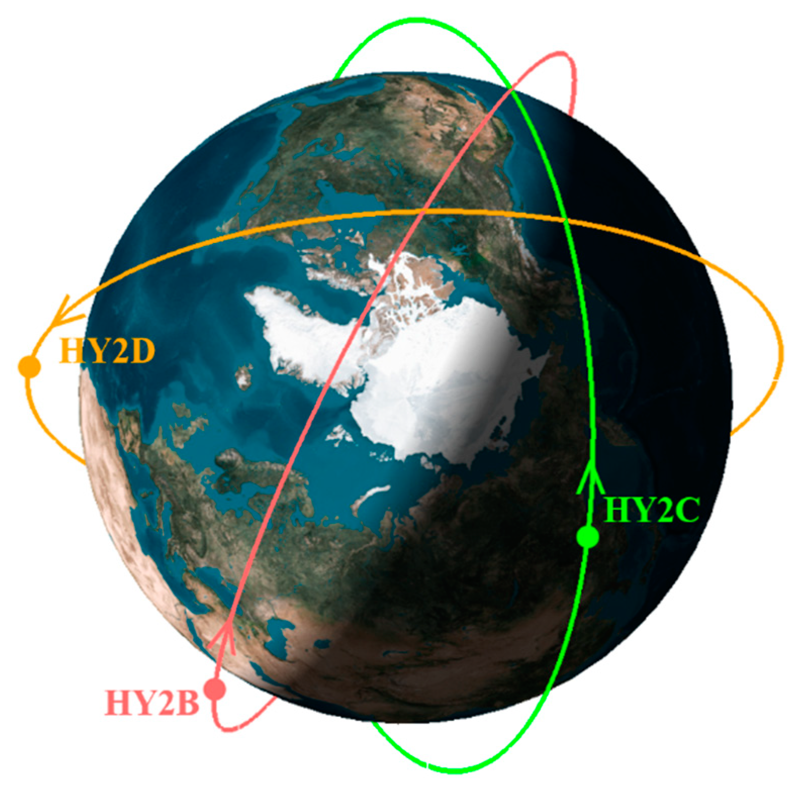
2.1. Datasets

The backscatter data contained in Level 1B (L1B) or Level 2A (L2A) products from Ku-band scatterometers onboard the spacecraft of HY-2B, HY-2C, HY-2D, QuikSCAT, and ISS were used. Table 1 provides brief information on these data products. We note that the σ 0 data from HY-2 scatterometers L1B products are used hereafter with an initial correction (provided in Table 1). The initial constant gain corrections are crudely estimated for each HSCAT instrument, and more precise and inter-calibrated corrections will be achieved based on this.
In addition, the NWP winds are from the European Centre for Medium-Range Weather Forecasts (ECMWFs) operational forecast model. The forecast time steps of +3 h, +6 h, …, +18 h are used in this study. The NWP data are quadratically interpolated with respect to time and bi-linearly interpolated with respect to geolocation. Note that small systematic differences exist between these standard ECMWF NWP 10-m winds and the more representative stress-equivalent 10-m winds [21], while these will be globally similar for all HY-2 wind datasets.

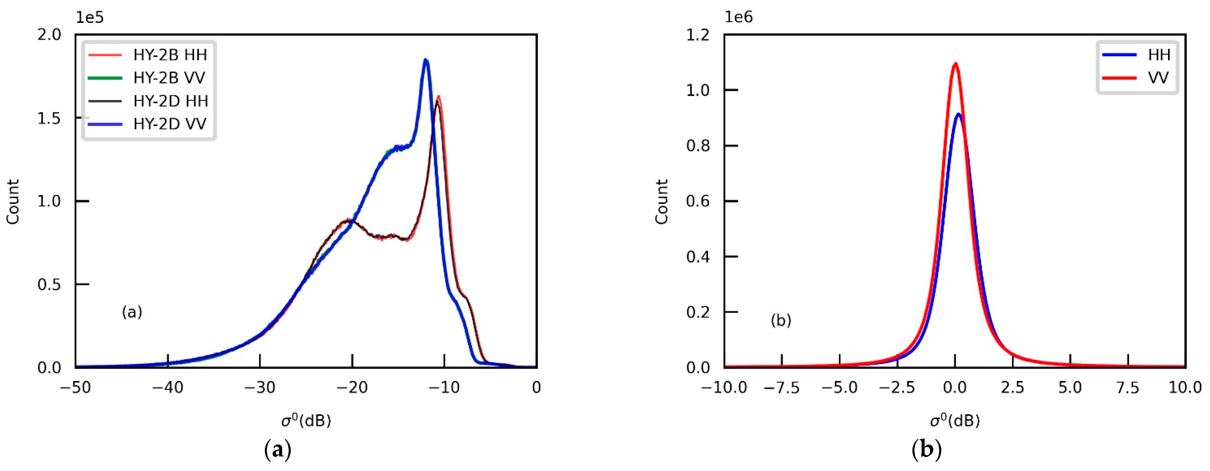
2.2. Direct Comparison Using Collocated Measurements

This method is based on the comparison of σ 0 data measured by two of the HSCAT scatterometers over the same area with a short time lag in order to limit geophysical changes to the scenes (in particular ocean wind speed and direction). The collocation constraints are: (1) the maximum spatial distance between pairs of σ 0 is 25.0 km; (2) the maximum temporal distance is 60 min; (3) and the maximum difference in antenna azimuth angle is 5°. In this study, the observing incidence angle is not a concern, since all the HSCAT instruments operate at the same fixed incidence angle. Figure 2 shows the global distribution of collocated HY-2B and HY-2D measurements in three months. The collocations are over land and oceans, and a few of them may be over sea ice. Besides, it is clear that there are more collocations near the latitude of 60° N or 60° S. This is because the HY-2D satellite only reaches latitudes within ±60°.
Based on the collocations, histograms of σ 0 values for each polarization can be generated. Then the probability density function (PDF) and cumulative distribution function (CDF) of σ 0 data for each polarization can be further made. Figure 3 provides the histogram of σ 0 data for the case of HY-2B and HY-2D, in which the σ 0 interval (horizontal axis) is 0.1 dB. It is clear that the curves of HY-2B and HY-2D are almost overlapping, and the histogram of corresponding differences is shown in Figure 3b for each polarization.
Based on the collocated backscatter measurements, the intercalibration result of the direct comparison method can be derived by two ways: (1) taking the average of differences between the collocated σ 0 data, i.e., the overall bias for each polarization; (2) and using a CDF matching technique to calculate σ 0 dependent calibration in dB units (i.e., corresponding to a nonlinear calibration for σ 0 in linear units).
The CDF matching method was applied in the derivation of the C-band model version 7 (CMOD-7) for sea surface wind retrieval, in which the CDF is for wind speed [8]. In this study, it will be applied to the CDF of σ 0 data. Two CDFs of σ 0 data can be matched in this way: one CDF is set as a reference and the other one is calibrated nonlinearly with respect to the reference. To each original (un-calibrated) data point σ o 0 a calibrated data point σ r 0 is associated, such that the original CDF value at σ o 0 equals the reference CDF value at σ r 0 . Thus, the calibration value at σ o 0 is σ o 0 σ r 0 .

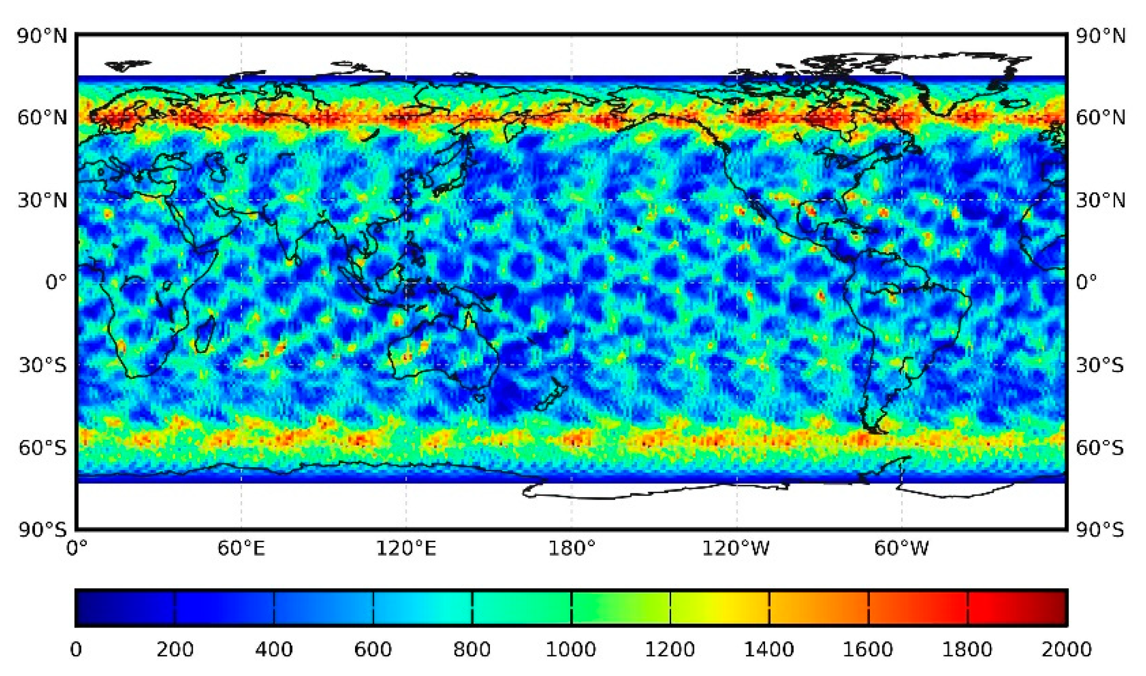
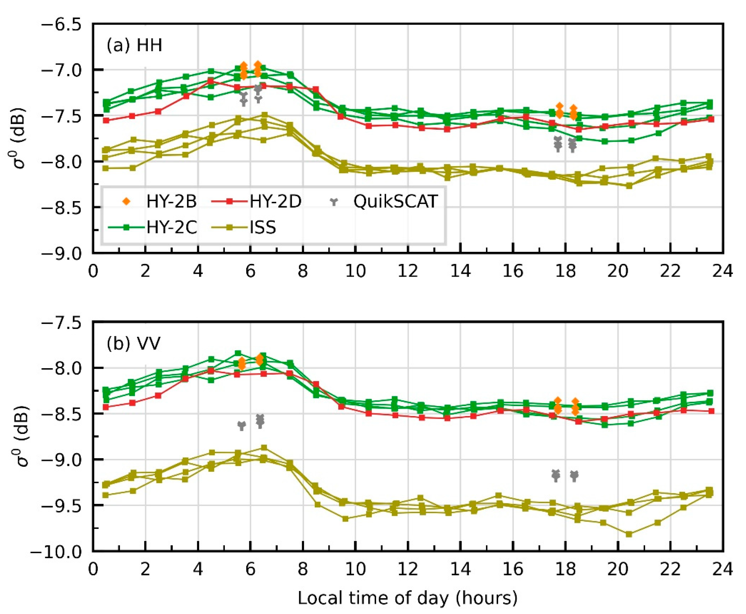
2.3. Intercalibration over the Amazon Rainforest

The Amazon rainforest is often used as a natural land target for the calibration of scatterometer σ 0 measurements, mainly because the azimuth dependence is negligible (less than 0.1 dB in magnitude) [19,22,23]. However, the annual, seasonal, and diurnal variations in σ 0 over the Amazon should be further investigated. In addition, the incidence-angle dependence of σ 0 over the Amazon rainforest is strong, but well-known and not a concern in this study [19].
The calibration target regions in the Amazon rainforest are defined by a spatial mask. In this study, a new Amazon mask, as shown in Figure 4, is defined based on HSCAT-B HH measurements in ascending passes in 2019. The σ 0 data are firstly binned into a regular grid (0.25° × 0.25°); then grid points with a standard deviation (SD) smaller than 0.5 dB are kept; lastly, some isolated grid points are manually removed (with less than three of eight kept as neighbor grid points). The new Amazon mask is different from the mask defined by the QuikSCAT data and used in [19], due to the rainforest declination, but the new one is fully contained in the older one.
The average annual σ 0 value of each grid point in the masked area in the Amazon is shown in Figure 4. Even though the annual variation in each grid point is less than 0.5 dB, the spatial distribution in the backscatter magnitude varies noticeably and ranges from −7.0 dB to −8.0 dB.
To estimate the annual, seasonal, and diurnal variations in σ 0 over the masked area in the Amazon rainforest, 9 years of QuikSCAT data, 33 months of HSCAT-B data, and 11 months of HSCAT-C data were used to generate Figure 5 and Figure 6.
Figure 5 provides the ten-day average of σ 0 measured by QuikSCAT (solid lines) and HSCAT-B (dotted lines) for different years, in which the yearly average was subtracted separately. Figure 6 provides the full diurnal variation in σ 0 for different seasons (winter (DJF), spring (MAM), summer (JJA), and autumn (SON)), which was measured by HSCAT-B, HSCAT-C, and RapidScat.
As we can see from Figure 5, the patterns of inter-annual variation are different from polarizations (HH or VV) and satellite passing orientation (ascending or descending). For QuikSCAT, the inter-annual variation in descending passes (6:00) is smaller than that of ascending passes (18:00). While for HSCAT-B, variation in descending passes (18:00) is stronger than ascending passes (6:00). The σ 0 differences between ascending and descending passes essentially come from the diurnal variations (as shown in Figure 6).
Figure 6 shows that the diurnal variation reaches 0.5 dB, which is much stronger than the seasonal or annual variation. There is a clear peak near sunrise (local time between 6:00 and 7:00 in the morning), and this can be attributed to the dew drops forming on leaves [24]. The diurnal variations shown in Figure 6 are in line with some previous studies [19,24,25,26].
It is clear from Figure 6 that the overall diurnal variations in ISS and HY-2 are quite similar, though the large vertical distances are caused by the incidence angle dependence and intercalibration, where QuikSCAT VV at 6:00 or 18:00 LST fits within the diurnal bounds. On the other hand, QuikSCAT HH and all HY-2 values are quite consistent. All HY-2 scatterometers provide measurements at 6:00 and 18:00, as dictated by the 6:00/18:00 LST orbit of HY-2B and HY-2A. Only HY-2C and HY-2D provide data at all LST. In this study, the relative calibrations are derived by comparing the data at local time around 6:00 and 18:00 in the following steps:
  • Average the σ 0 data for the local time in range of [5:00, 7:00] for each polarization. Then form the same average for σ 0 data in the local time range of (17:00, 19:00). The results are denoted as σ HH , 6 0 ,   σ HH , 18 0 ,   σ VV , 6 0 , and σ VV , 18 0 .
  • Compute the difference of average σ 0 values between two of HSCAT instruments at 6:00 and 18:00 separately for each polarization. The results are denoted as Δ σ HH , 6 0 ,   Δ σ HH , 18 0 ,   Δ σ VV , 6 0 , and Δ σ VV , 18 0 .
  • Compute the mean difference for the same polarization; the results are denoted as Δ σ HH 0 and Δ σ VV 0 .
Δ σ HH 0 = ( Δ σ HH , 6 0 + Δ σ HH , 18 0 ) / 2 ,
Δ σ VV 0 = ( Δ σ VV , 6 0 + Δ σ VV , 18 0 ) / 2 ,

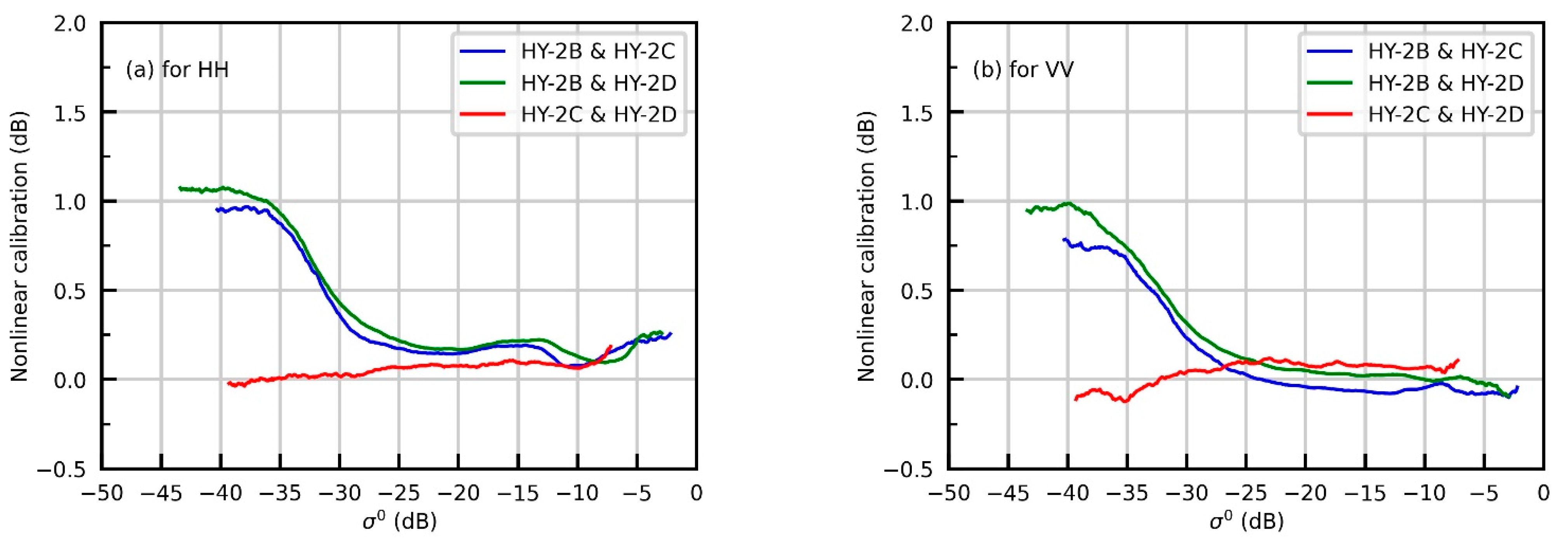
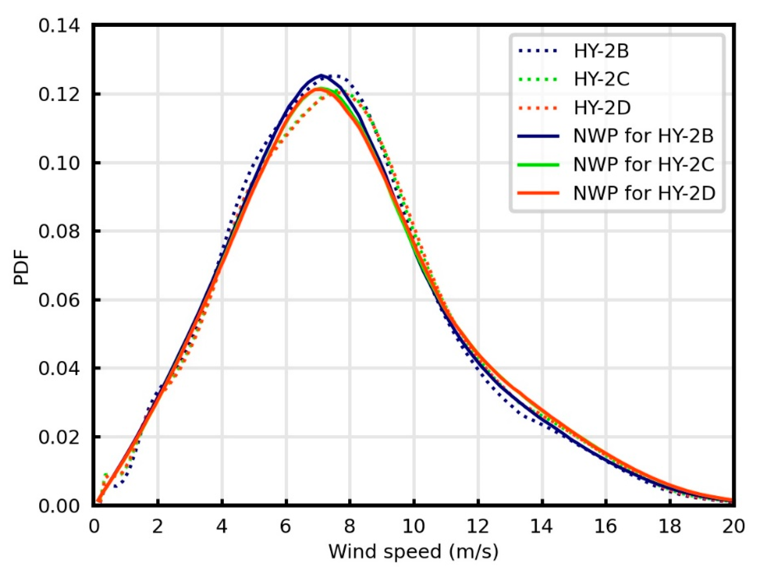
2.4. Double-Difference Technique Based on Backscatter Simulations over the Global Oceans

A backscatter calibration method based on numerical weather prediction (NWP) winds, called NOC, has been widely used for the calibration of spaceborne scatterometer measurements [20]. In this study, the double-difference technique is essentially the difference between the individual NOC results of two of the HSCAT instruments.
For each observed backscatter measurement ( σ o 0 ) over an ocean, the NWP wind can be matched. Then the simulated backscatter value ( σ s 0 ) can be computed via the NSCAT-4 geophysical model function (GMF) [27]:
σ s 0 = GMF ( V , φ , θ , p ) ,
where V is the sea surface wind speed, φ is the wind direction relative to the direction of radar antenna look, θ is the associated incidence angle, and p is the polarization. The NOC result ( Δ σ noc 0 ) is then defined as the distance between the observed and simulated σ 0 data for each polarization:
Δ σ noc 0 = σ s 0 ¯ σ o 0 ¯ ,
where σ s 0 ¯ and σ o 0 ¯ are σ 0 values that are first average over each wind direction in 6° bins, and then over all wind speeds with a weight proportional to the wind speed PDF over 1 m/s bins. In effect, the measured or simulated σ 0 are averaged over all wind azimuths weighted in accordance with a uniform wind azimuth distribution, and then they are averaged over all wind speeds weighted in accordance with the wind speed distribution.
The double-difference result is then defined as the difference between Δ σ noc 0 of two HSCAT instruments.

3. Results and Discussions

The intercalibration results obtained using the presented three methods are provided in Table 2. “Collocated” stands for the direct comparison using collocated measurements, “Rainforest” stands for intercalibration over the Amazon rainforest and “NOC” stands for the double difference based on backscatter simulations over the global oceans. In performing all methods, the same period (three months) of HY-2B, HY-2C, and HY-2D data were used.
As introduced above, the collocation method uses the CDF matching technique, and thus can generate nonlinear calibrations as a function of σ 0 value. Figure 7a,b shows the nonlinear corrections for HH and VV polarizations separately. We can see that the differences among HSCAT σ 0 data are small, particularly between HY-2C and HY-2D. However, the HY-2B σ 0 data below −25 dB shows noticeable separation against HY-2C or HY-2D. This can be related to the gain variation caused by the telemetric antenna temperature, noise processing, and different thermal conditions for the instrumentation in the different orbits (different solar illumination conditions). Note that backscatter values below −25 dB are relatively infrequent (see Figure 3a) and will mainly affect low wind speed retrievals over the ocean.
The HY-2B is in a sun-synchronous dawn-dusk orbit (6:00/18:00 LST), while HY-2C and HY-2D are in a similar asynchronous orbit with respect to the sun. This implies 2 groups of scatterometer with different sun irradiation conditions and hence different thermal space environments with possible effects on the calibration of noise and gain. The fact that the calibrations are different, does not imply correctness of one or the other, since both systems can, in principle, be varying due to thermal effects, but the variation along the orbits is rather similar for HY-2C and HY-2D. All scatterometers hence may be affected. At moderate winds, 0.1 dB bias implies 0.1 m/s wind speed error. At low winds, the amount of dB’s in 0.1 m/s increases. So, whereas the calibration bias below −25 dB increases, its effect on the wind speed error remains modest and only a few 10ths of a m/s. Integrating the backscatter PDF from low to high values corresponds to integrating the wind speed PDF from low to high values. So, below −25 dB implies about 10% of the lowest winds.
We furthermore considered that radar backscatter over land is relatively more stable than over the dynamic ocean in the collocation time window. However, we tested the direct comparison method for only the measurements over land or ocean, or for shorter time difference, where the results shown in Table 2 and Figure 7 only change negligibly (less than 0.05dB; not shown).
Figure 8 shows the hourly average σ 0 over the Amazon as measured by HH or VV polarization of HY-2B, HY-2C, and HY-2D scatterometers in summer. In performing the rainforest method, considering the diurnal variations, the scatterometer measurements that are used are limited to 5:00 to 7:00 and 17:00 to 19:00 according to local solar time.
The overall diurnal variations of HY-2C and HY-2D are clear, and the peaks are expected to occur around 6:00 near sunrise. However, this is not exactly the case for HY-2D. These results are assessed in the in-orbit test phase of scatterometers, while based on these results, further analyses of satellite gain and noise variations as a function of, inter alia, thermal conditions, will be useful. We do not have a clear explanation for that so far. Nevertheless, the σ 0 values over the Amazon near sunrise are very close.
The well-known NOC procedure was performed for HY-2B, HY-2C, and HY-2D measurements. In doing the NOC procedure, the simulated σ 0 are computed via the NSCAT-4 GMF with the ECMWF model operational forecast winds (real 10-m winds) as inputs. Figure 9 shows the PDF of ECMWF wind speeds matched for HY-2B, HY-2C, or HY-2D. Noting that the NOC is performed based on wind vector cells (WVCs), instead of the original individual σ 0 measurement contained in L1B product. The spatial size of a WVC is approximately 25 × 25 km2, which is closer to the ECMWF model resolution than the original σ 0 measurement. Besides, the normal quality control (QC) is applied to screen the data that may be contaminated by rain [28].
The PDFs of global wind speeds sampled by HY-2C and HY-2D are quite similar, while HY-2B shows noticeable differences from them. This is because the spatial coverage of HY-2C or HY-2D over a high latitude area is more frequent than HY-2B. Nevertheless, the differences in wind speed PDF have a limited effect on the NOC results.
In summary, the results among the three methods are comparable and their differences are roughly within 0.1 dB. The relative calibration values provided by the three methods are all small, which means the initial corrections (introduced in Section 2.1) for individual instruments are quite consistent.
To validate the appropriateness of all calibration results of the instruments, we compare the scatterometer winds with ECMWF model winds. Figure 10 shows the wind speed bias between HY-2 scatterometer and ECMWF model winds as a function of average wind speed. In the scatterometer wind retrieval processing, the same procedure (including NOC calibration, QC, GMF, and NWP auxiliary data) is followed for HY-2B, HY-2C, and HY-2D. The wind speed PDFs of scatterometer and ECMWF winds are shown in Figure 9.
As shown in Figure 10, the sea surface winds are very consistent among HY-2B, HY-2C, and HY-2D for wind speeds above 4 m/s and below 20 m/s, particularly between HY-2C and HY-2D. This is essentially in line with the results provided by the collocation method (shown in Figure 7). HY-2 scatterometer wind speeds are lower than ECMWF winds, and the biases increase as wind speed increases over the range from 8 to 18 m/s. In line with earlier studies [9,10,11,12], we conclude that this pattern is mainly caused by the NSCAT-4 GMF, the ECMWF wind input, and partly by the NOC results. Besides, the highest speed bins suffer from statistical sampling artefacts [29]. In particular, at high wind speed (>12 and <22 m/s) conditions, the wind speed biases compared with ECMWF winds among HY-2 scatterometers are all negative, since many high winds occur over cold sea surface temperatures, where the GMF produces too high a roughness at a provided input ECMWF wind speed. Conversely, backscatter values provide too low wind speeds after inversion over cold SST and hence the negative bias. Second, the ocean roughness responds to the local air mass density [21], which was not taken into account here and to atmospheric stability, which reduces the global wind by about 0.2 m/s, corresponding to approximately 0.2 dB [30]. Thirdly, different QC classes correspond to different backscatter biases with respect to the GMF, which is caused by the probability of the detection of rain and by the retrieval validation in enhanced wind variability conditions (without rain) [31]. Note in particular that enhanced wind variability near moist convection is not resolved by the ECMWF model [32] and the NOC in tropical rainy areas will therefore be offset. Finally, we note that both persistent small-scale and large-scale biases exist in the ECMWF model [32], such that satellites with different sampling may collect different NOC values. This latter effect appears small for the sampling difference between HY-2B and both HY-2C and HY-2D, since the NOC intercalibration effects are generally small for VV (Table 2). However, Table 2 shows that the backscatter intercalibration in NOC for the HH signal can reach 0.2 dB, which is not negligible.
The collocation method appears the most direct method of intercalibration, as it uses an identical weather sample for two instruments. For the rainforest and NOC method, different samples are chosen, but rather a fixed procedure is used. The rainforest method uses a relatively small domain with variable sampling and backscatter variations in time and location. NOC uses the global oceans as target and prior information on its variability, which is well forecast by ECMWF generally. However, we note that GMF errors and ECMWF model changes will affect NOC. Rainforest variability and errors related to NOC may cause uncertainty in the results. Using HY-2B as reference and the collocation differences as leading, one can compute the corrections for VV and HH for HY-2C as the sum of half the differences of HY-2B-HY-2C, HY-2B-HY-2D and HY-2D-HY-2C, resulting in −0.054 and +0.106 dB corrections, respectively. Similarly, for VV and HH of HY-2D, the sum of half the differences of HY-2B-HY-2C, HY-2B-HY-2D and HY-2C-HY-2D, result in +0.013 and +0.182 dB corrections, respectively. By applying these corrections for HY-2C and HY-2D, we obtain Table 3 based on Table 2.
One may note from Table 3 that the collocation differences with respect to HY-2B are within a few hundredths of a dB, similar to the relative accuracy of ASCAT and ERS calibration in measurement space [16]. The uncertainty in the rainforest calibration appears generally larger, in particular for HH against HY-2B. The different sampling of the scatterometers appears to introduce the largest uncertainty for the NOC method, particularly for VV. Nevertheless, in this representation all differences are well-below 0.1 dB for any method. Differences between HY-2C and HY-2D are particularly small between the different methods.
The small remaining uncertainty in the VV and HH calibration can potentially cause effects in the wind direction retrieval and in the mutual consistency of the measurements with the GMF. The latter is expressed in the wind retrieval residual and quantified as a maximum likelihood estimate (MLE), which is also used to detect geophysical anomalies for wind retrieval, such as rain [26]. Hence, small calibration changes in VV and HH, or VV with respect to HH, may affect QC, rain contamination, GMF definition, MLE values and wind speed and direction. These effects can be further investigated for all scatterometers after intercalibration.
Since the results of intercalibration provided by the collocation method and rainforest are comparable with NOC, almost the same curves of wind speed bias are expected for scatterometer winds using the calibrations provided by these methods. While the presented three methods for achieving intercalibration of scatterometer backscatter measurements are all effective, the rainforest and NOC methods depend on geophysical models of the rainforest or the ocean, which essentially ignore spatial and temporal variability effects. The collocation method proves very useful to obtain a more direct assessment of relative instrument calibration, more independent of geophysical variability effects, and to obtain an estimate of the uncertainty in the rainforest and NOC methods.

4. Conclusions

The number of satellite scatterometers is increasing, and consistencies of their sea surface wind products are critically important for data applications. In this study, we focus on the recently developed Chinese spaceborne scatterometer constellation, i.e., the Ku-band rotating pencil-beam scatterometer onboard the HY-2 series satellites. Three methods are presented and performed to achieve the intercalibration of backscatter measurements among the HY-2 scatterometers, which include: (1) direction comparison using the collocated backscatter measurements, in which the nonlinear calibrations can also be derived by using the CDF matching technique; (2) intercalibration over the Amazon rainforest; (3) and the double-difference technique based on backscatter simulations over global oceans, which essentially employs the calibration method called NOC.
In performing the direct collocation, a large number of collocations between HY-2 scatterometers are used over land, ice, and ocean and with a temporal difference less than 60 min. For the rainforest, considering the annual, seasonal, and diurnal variations in σ 0 data over masked Amazon rainforest, the scatterometer measurements that are used are limited from 5:00 to 7:00 and 17:00 to 19:00 according to local solar time. NOC is performed based on wind vector cells with a spatial size of 25 × 25 km2 instead of the original σ 0 data contained in L1B products.
The results among the three methods are quite close, and, when using the direct collocation method as reference, the differences are within 0.1 dB. To verify the results, scatterometer wind speeds are compared with the ECMWF model forecasts. It is shown that the curves of wind speed biases among HY-2 scatterometers are extremely close for wind speeds above 4 m/s and below 20 m/s. It is clear that the consistency of sea surface wind speeds among HY-2B, HY-2C, and HY-2D is well-established. Next, we can investigate the potential capability of these three methods to extend to all the spaceborne scatterometers and compare with cone metrics [16].

Author Contributions

Conceptualization, Z.W.; methodology, Z.W., J.Z. and W.L.; software, Z.W. and B.M.; validation, Y.Z. (Youguang Zhang); formal analysis, Z.W.; investigation, Z.W. and Y.Z. (Yi Zhang); resources, Y.H. and M.L.; data curation, Q.F. and J.Z.; writing—original draft preparation, Z.W.; writing—review and editing, Z.W. and A.S.; visualization, Z.W.; supervision, Z.W.; project administration, Z.W., Q.F. and J.Z.; funding acquisition, Y.H. and M.L. All authors have read and agreed to the published version of the manuscript.

Funding

This research was funded by National Natural Science Foundation of China, grant number 41906153, and partly by Key Special Project for Introduced Talents Team of Southern Marine Science and Engineering Guangdong Laboratory (Guangzhou), grant number GML2019ZD0302. Ad Stoffelen is supported by the EUMETSAT OSI SAF.

Institutional Review Board Statement

Not applicable.

Informed Consent Statement

Not applicable.

Data Availability Statement

The NSOAS ASCAT L1B data products are available at https://osdds.nsoas.org.cn/ (accessed on 1 September 2021). The QuikSCAT and ISS L2A data products are accessed from NASA PO.DAAC.

Acknowledgments

The authors would like to thank Jur Vogelzang, who is working on scatterometry at KNMI, for details and discussions in performing the CDF matching technique.

Conflicts of Interest

The authors declare no conflict of interest.

References

  1. Remund, Q.P.; Long, D.G. A decade of QuikSCAT scatterometer sea ice extent data. IEEE Trans. Geosci. Remote Sens. 2013, 52, 4281–4290. [Google Scholar] [CrossRef] [Green Version]
  2. Belmonte Rivas, M.; Otosaka, I.; Stoffelen, A.; Verhoef, A. A scatterometer record of sea ice extents and backscatter: 1992–2016. Cryosphere 2018, 12, 2941–2953. [Google Scholar] [CrossRef] [Green Version]
  3. Li, M.; Zhao, C.; Zhao, Y.; Wang, Z.; Shi, L. Polar sea ice monitoring using HY-2A scatterometer measurements. Remote Sens. 2016, 8, 688. [Google Scholar] [CrossRef] [Green Version]
  4. Turk, F.J.; Sikhakolli, R.; Kirstetter, P.; Durden, S.L. Exploiting over-land OceanSat-2 scatterometer observations to capture short-period time-integrated precipitation. J. Hydrometeorol. 2015, 16, 2519–2535. [Google Scholar] [CrossRef]
  5. Brocca, L.; Massari, C.; Ciabatta, L.; Wagner, W.; Stoffelen, A. Remote sensing of terrestrial rainfall from Ku-band scatterometers. IEEE J. Sel. Top. Appl. Earth Obs. Remote Sens. 2016, 9, 533–539. [Google Scholar] [CrossRef]
  6. Liu, W.T. Progress in scatterometer application. J. Oceanogr. 2002, 58, 121–136. [Google Scholar] [CrossRef]
  7. Ricciardulli, L.; Wentz, F.J. A scatterometer geophysical model function for climate-quality winds: QuikSCAT Ku-2011. J. Atmos. Ocean. Technol. 2015, 32, 1829–1846. [Google Scholar] [CrossRef]
  8. Stoffelen, A.; Verspeek, J.A.; Vogelzang, J.; Verhoef, A. The CMOD7 geophysical model function for ASCAT and ERS wind retrievals. IEEE J. Sel. Top. Appl. Earth Obs. Remote Sens. 2017, 10, 2123–2134. [Google Scholar] [CrossRef]
  9. Wang, Z.; Stoffelen, A.; Zhang, B.; He, Y.; Lin, W.; Li, X. Inconsistencies in scatterometer wind products based on ASCAT and OSCAT-2 collocations. Remote Sens. Environ. 2019, 225, 207–216. [Google Scholar] [CrossRef]
  10. Wang, Z.; Stoffelen, A.; Zou, J.; Lin, W.; Verhoef, A.; Zhang, Y.; He, Y.; Lin, M. Validation of new sea surface wind products from Scatterometers Onboard the HY-2B and MetOp-C satellites. IEEE Trans. Geosci. Remote Sens. 2020, 58, 4387–4394. [Google Scholar] [CrossRef]
  11. Wang, Z.; Stoffelen, A.; Fois, F.; Verhoef, A.; Zhao, C.; Lin, M.; Chen, G. SST dependence of Ku-and C-band backscatter measurements. IEEE J. Sel. Top. Appl. Earth Obs. Remote Sens. 2017, 10, 2135–2146. [Google Scholar] [CrossRef]
  12. Wang, Z.; Zou, J.; Stoffelen, A.; Lin, W.; Verhoef, A.; Li, X.; He, Y.; Zhang, Y.; Lin, M. Scatterometer Sea Surface Wind Product Validation for HY-2C. IEEE J. Sel. Top. Appl. Earth Obs. Remote Sens. 2021, 14, 6156–6164. [Google Scholar] [CrossRef]
  13. Wang, H.; Zhu, J.; Lin, M.; Zhang, Y.; Chang, Y. Evaluating Chinese HY-2B HSCAT ocean wind products using buoys and other scatterometers. IEEE Geosci. Remote Sens. Lett. 2019, 17, 923–927. [Google Scholar] [CrossRef]
  14. Elyouncha, A.; Neyt, X. C-band satellite scatterometer intercalibration. IEEE Trans. Geosci. Remote Sens. 2012, 51, 1478–1491. [Google Scholar] [CrossRef]
  15. Anderson, C.; Figa-Saldana, J.; Wilson, J.J.W.; Ticconi, F. Validation and cross-validation methods for ASCAT. IEEE J. Sel. Top. Appl. Earth Obs. Remote Sens. 2017, 10, 2232–2239. [Google Scholar] [CrossRef]
  16. Rivas, M.B.; Stoffelen, A.; Verspeek, J.; Verhoef, A.; Neyt, X.; Anderson, C. Cone metrics: A new tool for the intercomparison of scatterometer records. IEEE J. Sel. Top. Appl. Earth Obs. Remote Sens. 2017, 10, 2195–2204. [Google Scholar] [CrossRef] [Green Version]
  17. Bhowmick, S.A.; Kumar, R.; Kumar, A.K. Cross calibration of the OceanSAT-2 scatterometer with QuikSCAT scatterometer using natural terrestrial targets. IEEE Trans. Geosci. Remote Sens. 2013, 52, 3393–3398. [Google Scholar] [CrossRef]
  18. Zec, J.; Jones, W.L.; Alsabah, R.; Al-Sabbagh, A. RapidScat cross-calibration using the double difference technique. Remote Sens. 2017, 9, 1160. [Google Scholar] [CrossRef] [Green Version]
  19. Madsen, N.M.; Long, D.G. Calibration and validation of the RapidScat scatterometer using tropical rainforests. IEEE Trans. Geosci. Remote Sens. 2015, 54, 2846–2854. [Google Scholar] [CrossRef]
  20. Stoffelen, A. A simple method for calibration of a scatterometer over the ocean. J. Atmos. Ocean. Technol. 1999, 16, 275–282. [Google Scholar] [CrossRef] [Green Version]
  21. de Kloe, J.; Stoffelen, A.; Verhoef, A. Improved use of scatterometer measurements by using stress-equivalent reference winds. IEEE J. Sel. Top. Appl. Earth Obs. Remote Sens. 2017, 10, 2340–2347. [Google Scholar] [CrossRef]
  22. Kunz, L.B.; Long, D.G. Calibrating SeaWinds and QuikSCAT scatterometers using natural land targets. IEEE Geosci. Remote Sens. Lett. 2005, 2, 182–186. [Google Scholar] [CrossRef]
  23. Zhu, D.; Zhang, L.; Dong, X.; Yun, R.; Lin, W. Preliminary calibrations of the CFOSAT scatterometer. In Proceedings of the 2019 IEEE International Geoscience and Remote Sensing Symposium, Yokohama, Japan, 28 July–2 August 2019; pp. 8347–8349. [Google Scholar] [CrossRef]
  24. Satake, M.; Hanado, H. Diurnal change of Amazon rain forest/spl sigma//sup 0/observed by Ku-band spaceborne radar. IEEE Trans. Geosci. Remote Sens. 2004, 42, 1127–1134. [Google Scholar] [CrossRef]
  25. van Emmerik, T.; Steele-Dunne, S.; Paget, A.; Oliveira, R.S.; Bittencourt, P.R.; Barros, F.D.V.; van de Giesen, N. Water stress detection in the Amazon using radar. Geophys. Res. Lett. 2017, 44, 6841–6849. [Google Scholar] [CrossRef] [Green Version]
  26. Jaruwatanadilok, S.; Stiles, B.W. Trends and variation in Ku-band backscatter of natural targets on land observed in QuikSCAT data. IEEE Trans. Geosci. Remote Sens. 2013, 52, 4383–4390. [Google Scholar] [CrossRef]
  27. KNMI. NSCAT-4 Geophysical Model Function. Available online: https://scatterometer.knmi.nl/nscat4_gmf/ (accessed on 26 September 2021).
  28. Portabella, M.; Stoffelen, A. Rain detection and quality control of SeaWinds. J. Atmos. Ocean. Technol. 2001, 18, 1171–1183. [Google Scholar] [CrossRef]
  29. Stoffelen, A.; Vogelzang, J. Wind Bias Correction Guide. Document SAF/OSI/CDOP3/KNMI/SCI/GUI/390, NWPSAF-KN-UD-007, Version 1.5, 18-01-2021, KNMI, The Netherlands. Available online: https://nwp-saf.eumetsat.int/site/download/documentation/scatterometer/Wind_Bias_Correction_Guide_v1.5.pdf (accessed on 8 November 2021).
  30. Portabella, M.; Stoffelen, A. On scatterometer ocean stress. J. Atmos. Ocean. Technol. 2009, 26, 368–382. [Google Scholar] [CrossRef] [Green Version]
  31. Xu, X.; Stoffelen, A. Improved rain screening for ku-band wind scatterometry. IEEE Trans. Geosci. Remote Sens. 2019, 58, 2494–2503. [Google Scholar] [CrossRef]
  32. Belmonte Rivas, M.; Stoffelen, A. Characterizing ERA-Interim and ERA5 surface wind biases using ASCAT. Ocean Sci. 2019, 15, 831–852. [Google Scholar] [CrossRef] [Green Version]
Figure 1. The orbital positions of HY-2B, HY-2C, and HY-2D satellites at one moment.
Remotesensing 13 04783 g001
Figure 2. Global distribution of collocated HY-2B and HY-2D measurements for three months (June 2021 to August 2021). The color stands for the number of matchups in each 1° × 1° grid.
Remotesensing 13 04783 g002
Figure 3. Histogram of the matched σ 0 for each polarization of HSCAT-B or HSCAT-D (a), and the corresponding σ 0 differences (b). The histograms are counted with interval of 0.1 dB.
Remotesensing 13 04783 g003
Figure 4. Spatial mask defining the Amazon rainforest selected grid points. The color scale (in dB) depicts the average of the HSCAT-B HH measurements over 2019.
Remotesensing 13 04783 g004
Figure 5. Ten-day average σ 0 for the Amazon as measured by QuikSCAT (solid lines) or HSCAT-B (dotted lines) for different years. (a) for ascending passes, HH polarization; (b) for ascending passes, VV polarization; (c) for descending passes, HH polarization; (d) for descending passed, VV polarization.
Remotesensing 13 04783 g005
Figure 6. Hourly average σ 0 over the Amazon as measured by HSCAT-B, HSCAT-C, HSCAT-D, ISS/RapidScat, and QuikSCAT/SeaWinds for different seasons (different lines with the same color). Noting that only summer is available for HSCAT-D so far.
Remotesensing 13 04783 g006
Figure 7. The results of nonlinear calibration obtained using the CDF matching technique. It is masked if the number of samples in a bin (size of 0.1 dB) is less than 1000. (a) HH measurements, (b) VV measurements.
Remotesensing 13 04783 g007
Figure 8. Hourly average σ 0 over the Amazon as measured by HY-2B, HY-2C, and HY-2D in summer, 2021. Marker “■” stands for HH polarization, and “•” stands for VV polarization.
Remotesensing 13 04783 g008
Figure 9. Wind speed PDFs of HY-2 series scatterometer winds and the collocated ECMWF model winds.
Remotesensing 13 04783 g009
Figure 10. Wind speed bias between HY-2 scatterometer and ECMWF model winds as a function of average wind speed. The bin size is 0.5 m/s, and it is masked if the number of samples are less than 100 in a bin.
Remotesensing 13 04783 g010
Table 1. A brief description of datasets.
ScatterometerProductsInitial CorrectionsTime Period
HHVV
HY-2BL1B V20+0.5 dB−0.7 dBDecember 2018~August 2021
HY-2CL1B V20−1.3 dB−1.4 dBOctober 2020~August 2021
HY-2DL1B V22−0.6 dB−0.5 dBJune 2021~August 2021
QuikSCATL2A V2//January 2000~December 2008
ISSL2A V1.1//October 2014~August 2015
Table 2. Results of backscatter intercalibration among HY-2 series scatterometers.
CaseCollocatedRainforestNOC
HH (dB)VV (dB)HH (dB)VV (dB)HH (dB)VV (dB)
HY-2B and HY-2C+0.132−0.060+0.043−0.056+0.133+0.022
HY-2B and HY-2D+0.155+0.019+0.128+0.039+0.202+0.089
HY-2C and HY-2D+0.076+0.067+0.086+0.096+0.069+0.067
Table 3. Results of backscatter intercalibration among HY-2 series scatterometers after small dB corrections to HY-2C and HY-2D VV and HH (see text).
CaseCollocatedRainforestNOC
HH (dB)VV (dB)HH (dB)VV (dB)HH (dB)VV (dB)
HY-2B and HY-2C+0.0260.114−0.063−0.002+0.027+0.076
HY-2B and HY-2D−0.027+0.006−0.054+0.026+0.020+0.076
HY-2C and HY-2D0.0000.000+0.010+0.029−0.0070.000
Publisher’s Note: MDPI stays neutral with regard to jurisdictional claims in published maps and institutional affiliations.

