Development of an Electric Arc Furnace Simulator Based on a Comprehensive Dynamic Process Model


1
Department for Industrial Furnaces and Heat Engineering, RWTH Aachen University, Kopernikustr. 10, 52074 Aachen, Germany
2
Process Metallurgy Research Unit, University of Oulu, P.O. Box 4300, University of Oulu, 90014 Oulu, Finland
*
Author to whom correspondence should be addressed.
Processes 2019, 7(11), 852; https://doi.org/10.3390/pr7110852
Submission received: 22 October 2019
/
Revised: 8 November 2019
/
Accepted: 11 November 2019
/
Published: 14 November 2019
(This article belongs to the Special Issue Process Modeling in Pyrometallurgical Engineering)
Abstract
:A simulator and an algorithm for the automatic creation of operation charts based on process conditions were developed on the basis of an existing comprehensive electric arc furnace process model. The simulator allows direct user input and real-time display of results during the simulation, making it usable for training and teaching of electric arc furnace operators. The automatic control feature offers a quick and automated evaluation of a large number of scenarios or changes in process conditions, raw materials, or equipment used. The operation chart is adjusted automatically to give comparable conditions at tapping and allows the assessment of the necessary changes in the operating strategy as well as their effect on productivity, energy, and resource consumption, along with process emissions.
1. Introduction
The electric arc furnace (EAF) process is the main process for recycling of ferrous scrap [1] and the second most important steelmaking process route in terms of global steel production [2]. EAF process models have proven to be useful for improving process understanding and control as well as resource and energy efficiency by providing information that cannot be measured directly during the process due to the extreme conditions inside the furnace. Numerous models have been developed using different approaches both for the complete process as well as local phenomena or single process phases. However, few simulators allow for real-time manipulation of simulations by the user. Logar et al. [3] describe a simulator based on their process model and the World Steel Association provides an online EAF simulator on their website [4]. The simulator of Logar et al. [3] is based on a previously developed process model considering detailed heat transfer [5,6] and thermochemical equations [7] as well as an electrical model [8], whereas the World Steel Association gives only limited information about the workings of their model [9]. Other published models run simulations based on predetermined input data and although they can be used to study different scenarios, they do not adapt to current simulation results or user inputs.
In order simulate the process independent of plant data and cover extreme cases that may occur with unusual user input, a comprehensive mechanistic modelling approach is necessary. Several such models are available in the literature such as those of Bekker et al. [10,11,12] and MacRosty et al. [13,14,15] who introduced some of the simplifications and assumptions that Logar et al. based their model on, as well as several others that have been published with a varying degree of detail [16,17,18,19,20,21,22,23,24,25,26,27,28,29,30,31]. Both Meier et al. [32,33,34,35,36,37] and Fathi et al. [38] have published models developed on the basis of the work of Logar et al. [3,5,6,7,8]. With the exception of Logar et al., all these models rely on predetermined input from measured data and, as far as can be determined from the published information, no other simulators that provide direct feedback and control for the user are available. Meier implemented the automatic control of the model on the basis of current simulation results [35], but his model does not allow direct user input during the simulation. The model and simulator presented here are based on a further development of the model proposed by Meier [39]. Although the general model structure and most of the assumptions and simplifications from Logar et al. [3,5,6,7,8] remain, the model has been adjusted for a different solver algorithm [36] and substantially modified [32,33,34,36,37,39] making it one of the most comprehensive and up-to-date EAF process models currently available. The differences compared to the model published by Logar et al. include a more efficient numerical method for solving the model equations [36], increased detail in the gas phase with additional species and reactions [34,37], a more comprehensive model of the radiative heat transfer considering the influence of the gas phase [32,37], the treatment of different carbon carriers [33], and the refinement of the thermochemical model for the interaction of slag and melt with each other as well as the injected oxygen and carbon [39].
2. Process Model
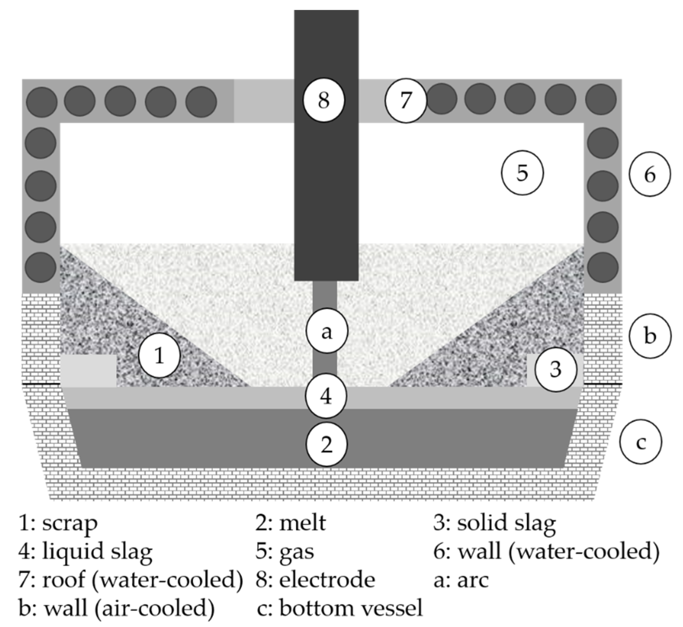
The model presented here as a basis for the simulator is essentially the state of development documented in a previous publication [39]. The model is executed in the MATLAB environment. Within the model there are eight different zones (i.e., control volumes), each of which is homogeneous in terms of composition and temperature. Separate energy and mass balances are defined for each zone. The zones are the (1) solid scrap, (2) liquid metal, (3) solid slag formers, (4) liquid slag, (5) gas phase, (6) water cooled wall and roof, and (8) the electrode(s). The electric arc is treated simply as a heat source whereas the air-cooled bottom vessel and lower wall section are represented as heat sinks. Figure 1 shows a schematic illustration of all zones and heat sinks/sources within the model.
Relevant phenomena such as heat exchange through radiation and direct contact, phase changes and mass transfer between zones, chemical reactions, as well as the change in geometry during meltdown, are considered in the model. Simulation results have been validated using extensive data from industrial furnaces [32,33,34,37,39].
The operation of the furnace is characterized by continuous as well as discontinuous mass and energy flows. For the charging of scrap baskets, the amount and composition of scrap, slag formers, and coal charged with each basket can be considered with an unlimited number of baskets per heat. The charging in bulk of coal, slag formers, or alloys without scrap can be accounted for as well by defining the desired amount and composition and charging it independently. Due to the discontinuous change of conditions inside the furnace resulting from charging of material in bulk, the integration is stopped and restarted with new initial values adjusted according to the added material for each charging event.
The time-dependent model input or operation chart consists of the electric energy input characterized by voltage and current as well as the mass flows of oxygen for lances, burners and post-combustion, natural gas for burners, coal for carbon lancing, slag former injection, and off-gas extraction. The cooling of the wall and roof is determined on the basis of the mass flows and inlet temperature of the respective cooling water flows. For the simulation based on plant data, these inputs are determined from measured values or estimates and stored for each heat at the beginning of the simulation to be evaluated at every time step of the simulation. Additional parameters describing furnace-specific properties such as the geometry and empirical factors adjusted for each individual plant are stored in a separate Excel file. Different parameter sets can be defined and automatically simulated in succession. By comparing the results for different parameter settings, empirical parameters can be adjusted for different furnaces or process conditions and the impact of parameters such as the composition of slag formers or coal and gases can be evaluated. For the automatic control of the simulation as implemented by Meier [35], the masses charged in bulk are predetermined while the time of charging, mass flows, and electric energy input are determined on the basis of the progress of the simulation and rules derived from the operation of a real-life furnace. For the simulator, the operation chart and charging of baskets can be determined by the user during the simulation.
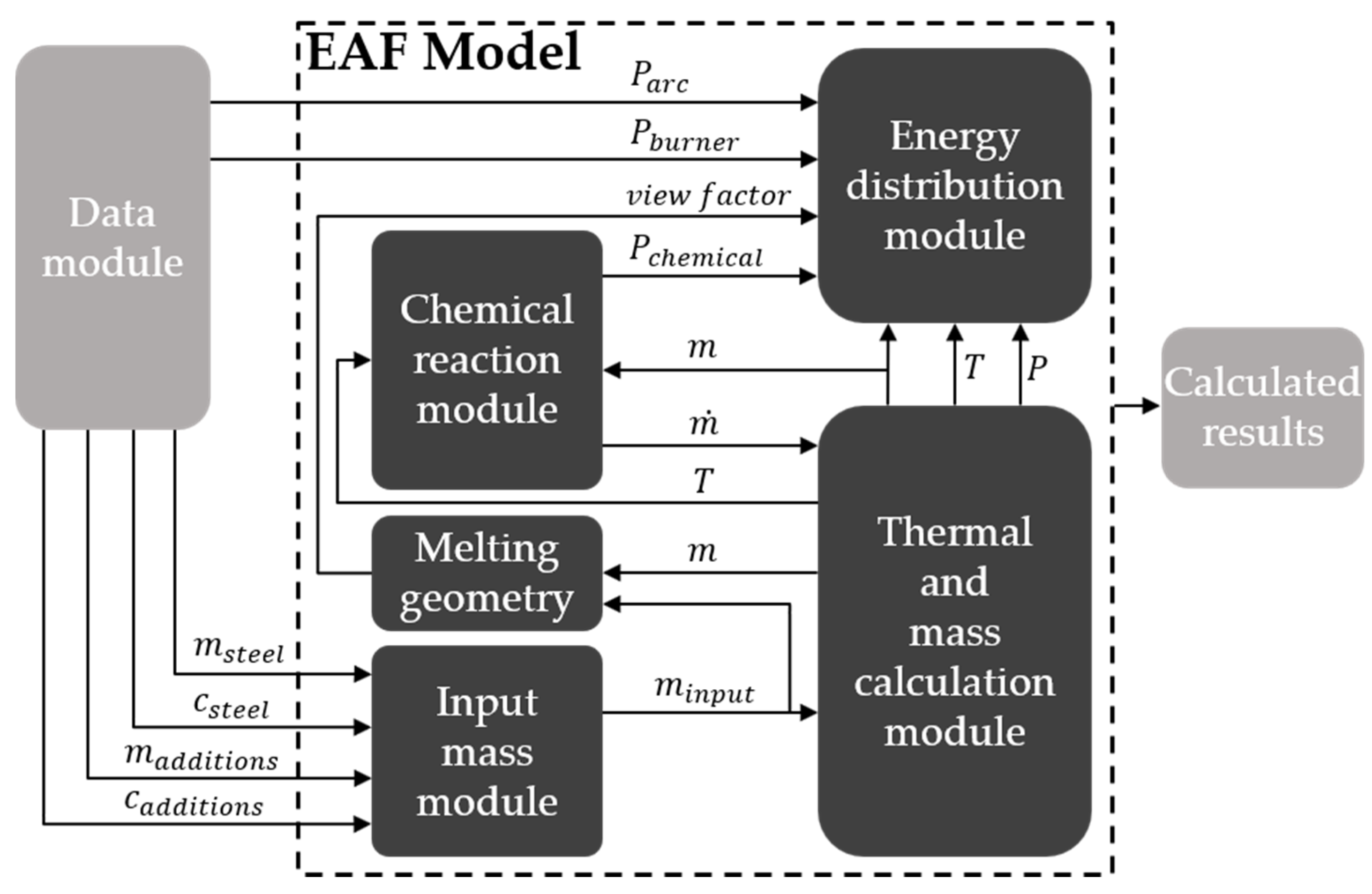
Figure 2 shows the structure of the model with its different modules and the exchange of information between them. Essentially, the main model runs independent from the type of data use and the change between the three running modes (measurement-based simulations, automatic control, and user-input-controlled simulations) affects only the data module and its interaction with the main model.
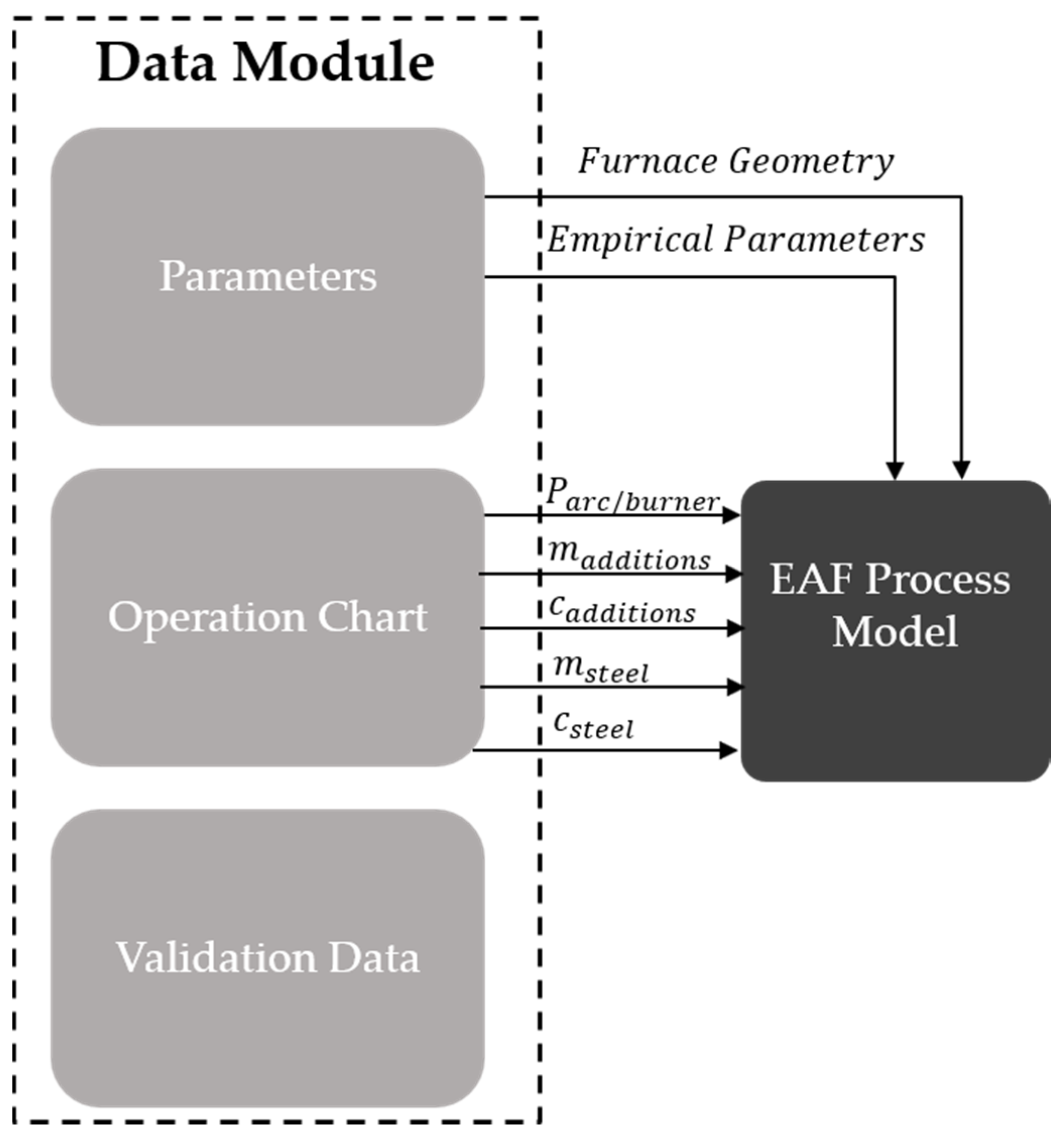
The data module determines both the initial conditions for each basket that are calculated in the input mass module and the time-dependent input during the simulation that is transferred to the energy distribution module for each time step. Figure 3 shows how the structure of the data module and the data that is exchanged with the EAF model when measured data is used. The input is predetermined for each point of time and together with the geometry and other furnace-specific parameters determines the input for the model. The validation data is not used directly as model input but can be compared to model results and to adjust empirical parameters.
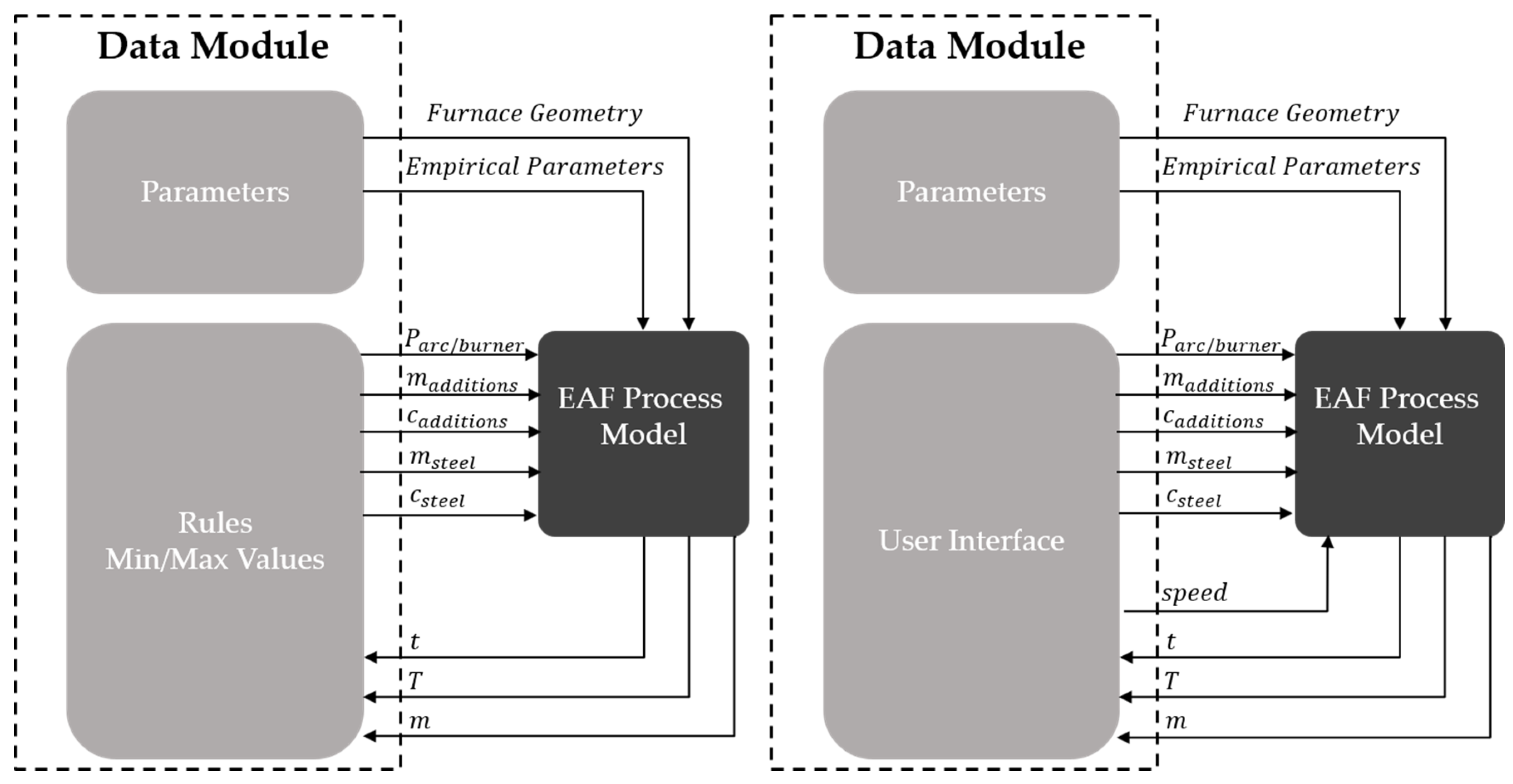
Figure 4 shows the structure of the data model for the automatic control (left) and simulator (right) modes. Because the input is no longer predetermined for the full simulation, the time and current state have to be passed back to the data module for each step. In the case of the automatic control mode, the current input is then determined on the basis of the current set of parameters, rules, and minimum/maximum values and passed back to the EAF model. In the simulator mode, the user interface is updated with the current model results and the input for the model is updated with those set in the interface so that any changes made by the user since the last update are carried over to the EAF model. Furthermore, for the simulator mode, the selected speed is passed to the model as an additional input parameter, whereas in all other cases the model always runs with the highest attainable speed by default.
3. Automatic Control Mode
The automatic control mode of the simulation implemented by Meier [35] was developed to evaluate different scenarios such as the use of alternative materials of varying quantity and composition, for instance, the replacement of coal with alternative carbon carriers and the use of oxygen from different sources with varying oxygen and nitrogen content, or different operating strategies for the control of post-combustion, burners, and carbon and oxygen lances. The simulations are automatically adjusted to reach the predetermined conditions at tapping for all scenarios so that their impact on energy consumption, operating cost, and carbon emissions can be evaluated.
3.1. Input
Different scenarios for which automatic operating strategies are to be generated and compared can be defined by the user in an additional worksheet of the Excel file used for the furnace parameters. First, the masses and compositions of scrap, two coal types, and two slag formers (usually lime and dolomite) charged with three scrap baskets are defined. Although the input file is currently limited to this, the model allows the addition of both more baskets and additional types of coal or slag formers. The scrap composition can be defined separately for each basket. Furthermore, the initial conditions before charging of the first basket, namely, the mass, temperature, and composition of the hot heel present in the furnace have to be set. In addition to the values defining the initial conditions and charged material, the minimum and maximum values have to be set for the electric power and voltage, oxygen input for lances, post-combustion and burners, carbon injection, off-gas mass flow, slag former injection, natural gas for burners, and the voltage. The variation of these parameters between the selected minimum and maximum values over the course of each simulation is determined according to a set of rules that in turn can be adjusted through the parameters shown and described in Table 1.
One minimum and several maximum values can be given for each parameter. The model automatically selects all possible combinations and runs a simulation for each case. This can be combined with the variation of parameters, such as the composition of coal and slag formers, allowing a large number of scenarios to be simulated and compared automatically.
3.2. Control of Operation Chart Parameters
Using predefined rules, the model determines the desired value for each parameter from the selected minimum and maximum values during the simulation, replacing the fixed operation chart determined from measured data. The rules are derived from the current operating strategies and operation charts from the regular operation of different EAF. The simulation starts with the charging of the first basket and is terminated after the scrap charged with the final basket has melted and a predefined carbon content and temperature of the melt have been reached. After and before the charging of each basket all values of the operation chart are set to their minimum (power off) values for the delays defined by tstart-delay and tstop-delay to account for the power-off time associated with the raising and lowering of the electrodes, as well the opening and closing of the roof as necessary, when scrap is charged into the furnace. The condition for charging the next basket is that the sum of the currently remaining solid scrap volume and the volume of the scrap charged with the next basket are below the maximum allowed scrap volume Vscrap-max. If no additional basket is defined and the conditions for tapping are met, all operation chart parameters are reduced to their minimum values and the simulation is terminated. The charging of the second and additional baskets is triggered by an event function that constantly checks if the necessary conditions have been met. Initially, once the conditions are met for charging of the next basket, all operation chart parameters are reduced to their respective minimum values and the simulation continues until tstop-delay has passed. The simulation is then stopped and reinitiated with new starting values and continues with a power-off period determined by tstart-delay and the following power-on period just as with the first basket.
A hyperbolic tangent function is used to allow rapid but continuous changes between states where necessary. It can assume values between one and zero and is based on a controlling variable and a threshold. φ(a,b) indicates a hyperbolic tangent function that has the value zero as long as the variable a is smaller than the threshold b, and rapidly changes to one if a increases to values higher than b. For example, the factor indicating the charging of the next basket would be based on the maximum allowed scrap volume Vscap-max, the scrap volume in the next basket Vscrap-next, and the actual scrap volume Vscrap, as shown in Equation (1):
Φbasket = φ (Vscrap,Vscrap-max − Vscrap-next).
It would become zero once the free volume is large enough to charge the next basket. Such factors are used for all conditions and delays defining the operation chart.
The electric power is reduced for the initial period after charging until bore down has progressed far enough to allow the arc to burn inside the scrap, at which point significantly less radiation is received by the wall and roof, and maximum power can be used. Later during the process, power is reduced once the full bath surface is uncovered and the flat bath phase begins. During any stage of the process, the power will be reduced if the wall temperature reaches the critical temperature Twall-crit. The voltage is assumed to be a linear function of the power and the current is determined accordingly.
The oxygen lance mass flow is initially set to the percentage defined by Olance-min and increases once the burner power conditions set by Clance-burner is fulfilled with another increase to its maximum value once the complete bath surface is free of solid scrap. The ratio of the first and second increase is determined by the parameter Clance-bath. Post-combustion oxygen flow is started with the maximum value once the additional delay tpost-delay has passed and a minimum of 5% of the scrap has melted. It is stopped once the mass of solid scrap remaining divided by the initial amount of scrap has reached Cpost-scrap. The burners are started with full power and both oxygen and natural gas input are stopped once the remaining scrap has reached Cburner-scrap. Carbon injection is started after meltdown of the last scrap charge has progressed far enough to create a free bath surface as defined by Ccarbon-bath. Once the melt temperature approaches the desired tapping temperature or the amount of remaining scrap reaches Ccarbon-scrap, carbon injection is phased out. Oxygen lancing is reduced proportionally with the reduction in carbon injection.
Off-gas extraction is started at the minimum mass flow and increased with the injection of gases and carbon. Because the injection of slag formers using lances is not practiced at the furnaces this automatic control was initially designed for, no rules have been defined for this purpose and the mass flow is permanently set to zero. The practice could, however, be included by simply defining the necessary factors and rules, as the process model does include the necessary equations and simulations based on measured data have been run successfully for furnaces where the injection of lime is practiced. Cooling water flows and inlet temperatures are assumed to be constant for these simulations.
4. Simulator Mode
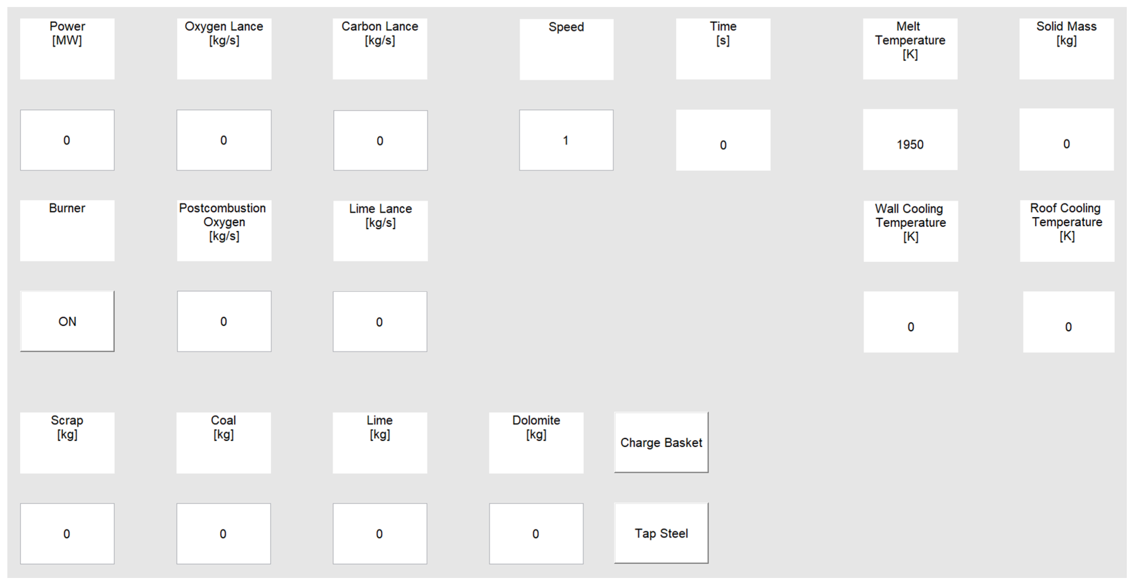
Direct real-time feedback and control are necessary for the simulator function. Therefore, a user interface has to be implemented to control the simulator and display current results while the simulation is running. Figure 5 shows the currently used interface which displays the simulation time, current melt temperature, remaining solid scrap mass, and the cooling water outlet temperatures of wall and roof to indicate the progress of the process. The user can enter values for electric power, oxygen, carbon, and lime injection, and select burners ‘on’ or ‘off’ to control the simulation. The button ‘charge basket’ allows for the charging of the masses selected for scrap, coal, lime, and dolomite in the corresponding fields.
The model allows the display of any value calculated during the simulation, parameters such as the total energy consumption or off-gas composition and temperature that can be used for control of industrial furnaces that can easily be added to the display. The same is true for information that is not attainable for a real-world furnace such as temperatures and energy or mass flows inside the furnace. Furthermore, every operation chart parameter can be added and manipulated by the user. Values for off-gas mas flow, arc voltage, and cooling water flows are currently set automatically but could be added to the interface instead. Simulations are started by charging the first basket and ended using the button ‘tap steel’. Pressing these buttons during the simulation triggers an event and the sequence of determining new starting values and reinitiating the integration, which is described for the simulation using measured data or automatic control.
4.1. Simulation Speed
The EAF model runs simulations significantly faster than the real process times—the process taking roughly one hour per heat in reality can be simulated in less than a minute using a tabletop computer (3.4 GHz, 4 core central processing unit, 32 GB random-access-memory). In order to allow the user to make inputs and evaluate the current results, the simulation has to be slowed down. Therefore, the simulation is paused after each second of simulated process time, the user interface is updated, and values changed by the user after the previous update are returned to the process model. The duration of the pause depends on the actual speed of the simulation and the desired speed set by the user. If the simulation is progressing slower than the desired simulation rate, the pause is set to the smallest possible value that allows the user interface to be updated. Otherwise, the pause is held long enough to allow the simulation to synchronize with the desired simulation rate. The simulation speed can be adjusted by the user during the simulation.
4.2. Model Adjustments
Due to the different nature of the simulation input, several changes to the model and solver are required to insure fast and stable operation when using the simulator. When measured data is used as input, the operation chart values can be interpolated between time steps and the full operation chart is available at all times. For the automatic control, smooth changes are insured through the use of a hyperbolic tangent function and the rules remain the same throughout the simulation, allowing for stable simulation. Furthermore, both the automatic control and measured data from industrial operation usually insure smooth and consistent progression of the process, whereas with the simulator erratic user inputs and far more extreme and unusual states can be encountered, posing a significant challenge for the process model.
4.2.1. Continuity of Operation Chart
When using the simulator, the model has to be adjusted for unpredictable and discontinuous changes in operation chart values due to user input. Whenever such sudden changes are detected by the ODE15s solver used for the EAF model, negative time steps can occur, meaning that the solver will jump back to an earlier time and recalculate with a smaller step-size. Therefore, it is not possible to always use the value currently set in the interface. Instead, the operation chart is extended with the current time and values every time the interface is updated, and if negative steps occur then the previous values are used accordingly.
4.2.2. Pressure Oscillations
In rare cases, usually when reinitiating electric energy input after long power-off periods, the calculated pressure can start oscillating, causing the simulation to become very slow and eventually crash. This is caused by a feedback loop from the coupling of leak air ingress with the pressure and temperature of the gas phase. The pressure is calculated using the ideal gas law according to Equations (2) and (3):
where P is the pressure, t is the time, T is the gas phase temperature, R is the gas constant, and mi and Mi are the masses and molar masses of species in the gas phase, respectively. V is the volume of the gas phase and is assumed to remain constant, whereas the mass of the gas phase depends on the density and composition of the gas.
The leak air intake is assumed to be a linear function of the pressure inside the furnace, as shown in Equation (4):
where a, b, and c are empirical parameters fitted to match measured data and optimize stability. In some cases, an increased intake of leak air will cause the temperature to drop, with a resulting reduction in pressure that in turn will increase the leak air ingress and vice versa. This can lead to unstable behavior and pressure oscillations with large amplitudes. This problem was addressed by defining the leak air ingress as a differential variable according to Equation (5).
This allows the solver to detect steep changes in the leak air intake and adjust the time-step accordingly so that oscillations can be avoided. The difference in simulation results between Equations (4) and (5) is negligible.
4.2.3. Additional Stability Improvements and Model Acceleration
In addition to the pressure oscillations, certain unusual cases exist where masses would reach small negative values causing the model to crash. This was rectified by using the ‘NonNegative’ option of the ODE15s solver to insure the necessary adjustments of time-steps when masses approach zero with a steep gradient and the adjustment of some empirical model parameters, especially in several hyperbolic tangent functions that reduce chemical reaction rates when the mass of a reactant is small. Furthermore, the model was accelerated by making the integration more efficient. The ODE15s solver numerically calculates a Jacobian matrix that leads to a high number of function evaluations with a single variable changing. By detecting this behavior and using previous results for expensive analytical calculations, such as the determination of chemical activities and radiative heat transfer, if none of the relevant inputs have changed, the simulation speed is increased significantly. Furthermore, the number of function evaluations could be reduced by using the ‘JPattern’ option. Overall this made the simulation more stable and significantly faster [39]. Crashes or non-physical results such as negative masses have not been observed with the new model, even with unrealistic inputs and extreme conditions.
5. Results and Discussion
Validation of the EAF process model using extensive measured process data from a 140 t direct current (DC) furnace can be found in previous publications where the thermochemistry of the gas phase [34] and liquid phases [39], the behavior of different carbon carriers [33], the heat transfer [32], as well as the performance of the complete model [37], were evaluated thoroughly, which is not reproduced here. The model has also been tested with data from additional furnaces including both alternating current (AC) and DC technology and has given satisfactory results after adjustment of the empirical parameters during preliminary research. Instead, various simulations where both were run in automatic control and simulator mode were set up to evaluate the model stability and speed as well as its capability to reproduce existing operation strategies and adjust them for an altered set of boundary conditions.
5.1. A Case Study for Different Operating Modes
The automatic control was initially adjusted to reproduce the results obtained from simulations with measured data. Inputs with the scrap baskets as well as maximum and minimum mass flows were set to match those documented for an industrial 140 t DC furnace. After adjusting the automatic control to match the simulation on the basis of measured data for the operation chart, a scenario was tested where the oxygen used for the furnace operation was taken from a different source with an oxygen content of 40% instead of the 99% used for the initial case, with the remaining fraction consisting of nitrogen in both cases. The mass flows for oxygen lancing, burners, and post-combustion were adjusted to have the same mass flow of pure oxygen. Due to the decreased oxygen content, this led to an increased total mass flow and more nitrogen being injected together with the oxygen. The operation chart was automatically adjusted to reach the same tapping temperature and maximum carbon content, resulting in an increased energy consumption (both electrical and chemical) and an increased tap-to-tap time. The following cases were studied:
- Case 1, indicating the results obtained by adjusting the automatic control to reproduce the measured operation chart;
- Case 2, indicating the results from the same control settings with the decreased oxygen content.
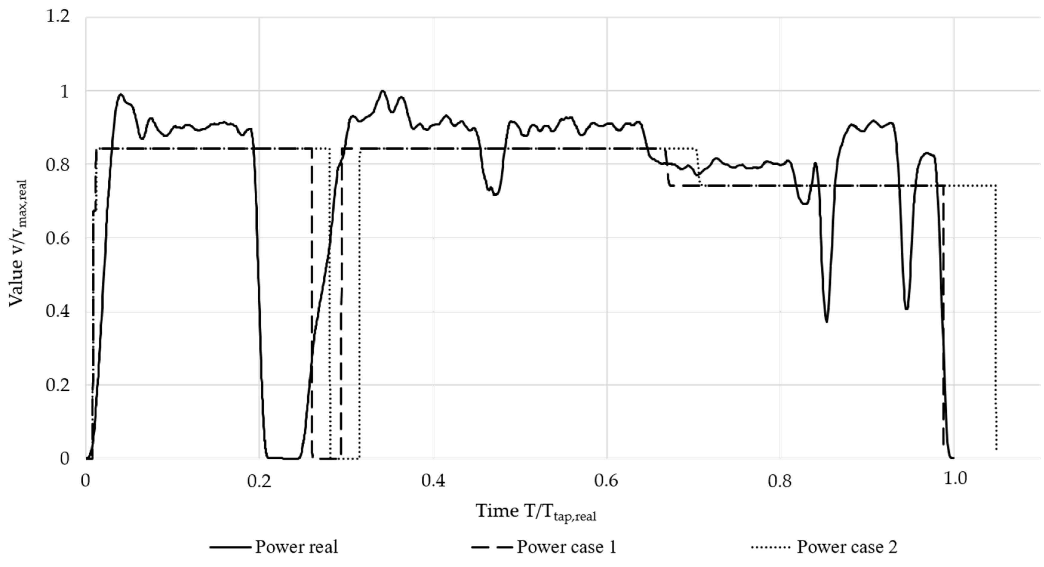
The oxygen shown in the following discussion is the actual mass of pure oxygen; therefore, between Case 1 and Case 2 the total oxygen consumption increased by 6.5%, whereas, due to the increased nitrogen fraction, the nitrogen carried into the furnace with the injected oxygen for Case 2 was 64 times that of Case 1. Figure 6 shows the measured electrical power (real) during the heat compared to the automatic control for Case 1 and Case 2. The time was normalized using tap-to-tap time of the measured heat, the power was normalized using the maximum measured value.
Although the measured value fluctuated, the automatic control gave constant values. This had little impact on the overall consumption if the mean measured power was selected for automatic control. As can be seen from the reduction in power to zero, for the measured heat, the second basket was charged at about 0.23 process time, whereas automatic control charging occurred at roughly 0.3 for Case 1 and slightly later for Case 2. The time when the second basket was charged depended on the initial density of the scrap as well as other parameters, which could vary between baskets, and the progression of the process was not reproduced exactly here. Therefore, the reduction of power and mass flows associated with the charging of the second basket occurred slightly later in the simulations when compared to the measured operation chart. At about 0.65 and 0.7, the power was reduced for the flat bath phase for Case 1 and Case 2, respectively.
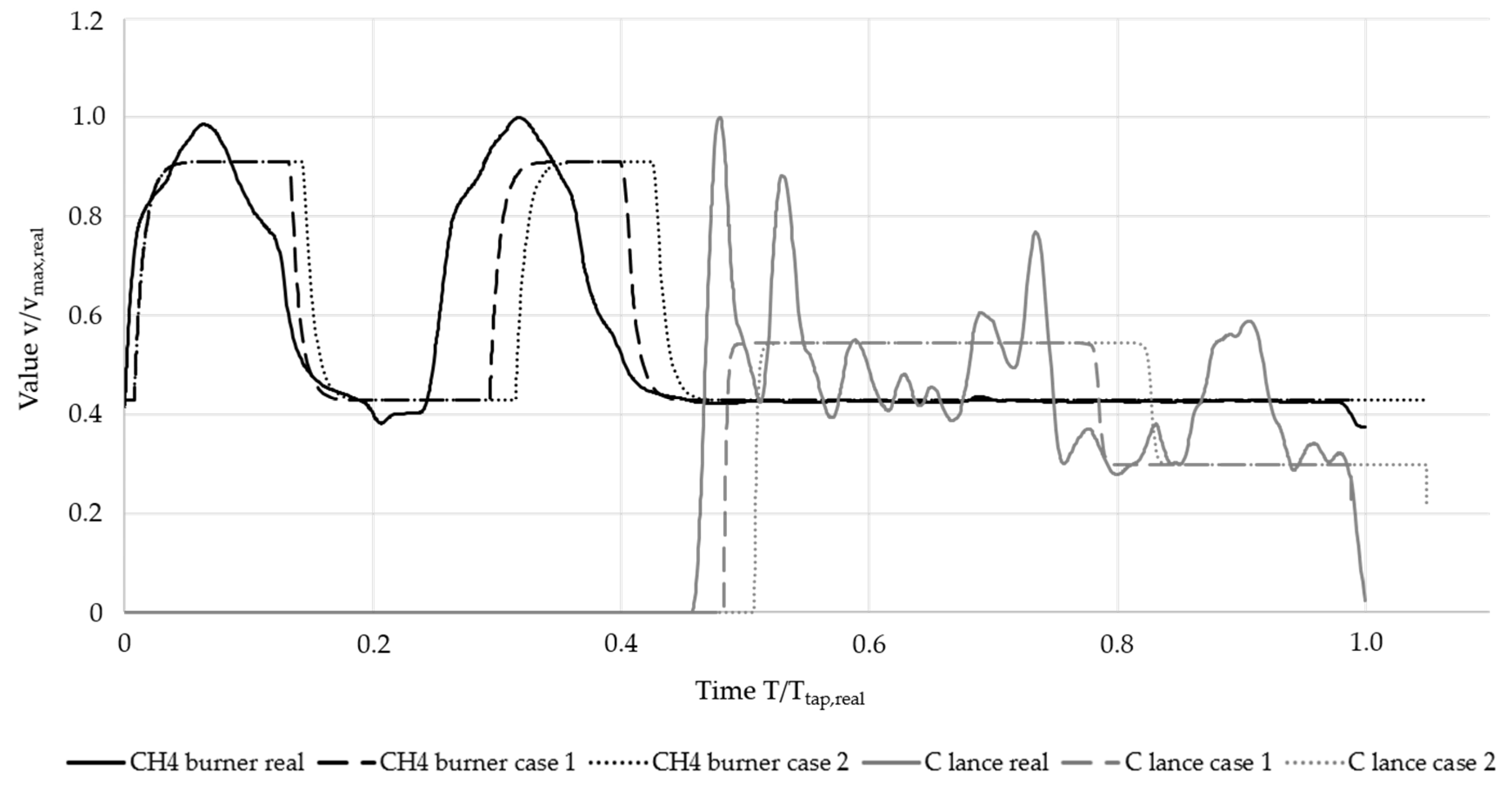
Figure 7 shows the consumption of natural gas denoted by CH4 and injected coal denoted by C for the measured heat and Cases 1 and 2. Mass flows and time were normalized the same way as in Figure 6. For the first basket, the burners both in Case 1 and Case 2 showed almost identical behavior as was measured. Due to the delayed charging of the second basket, burner operation was delayed as well for the second basket, with a larger delay for Case 2 as meltdown of the initial basket was slower when compared to Case 1. Carbon lancing started slightly later than for the measured operation chart and the mass flow was reduced at around 80% of the process time.
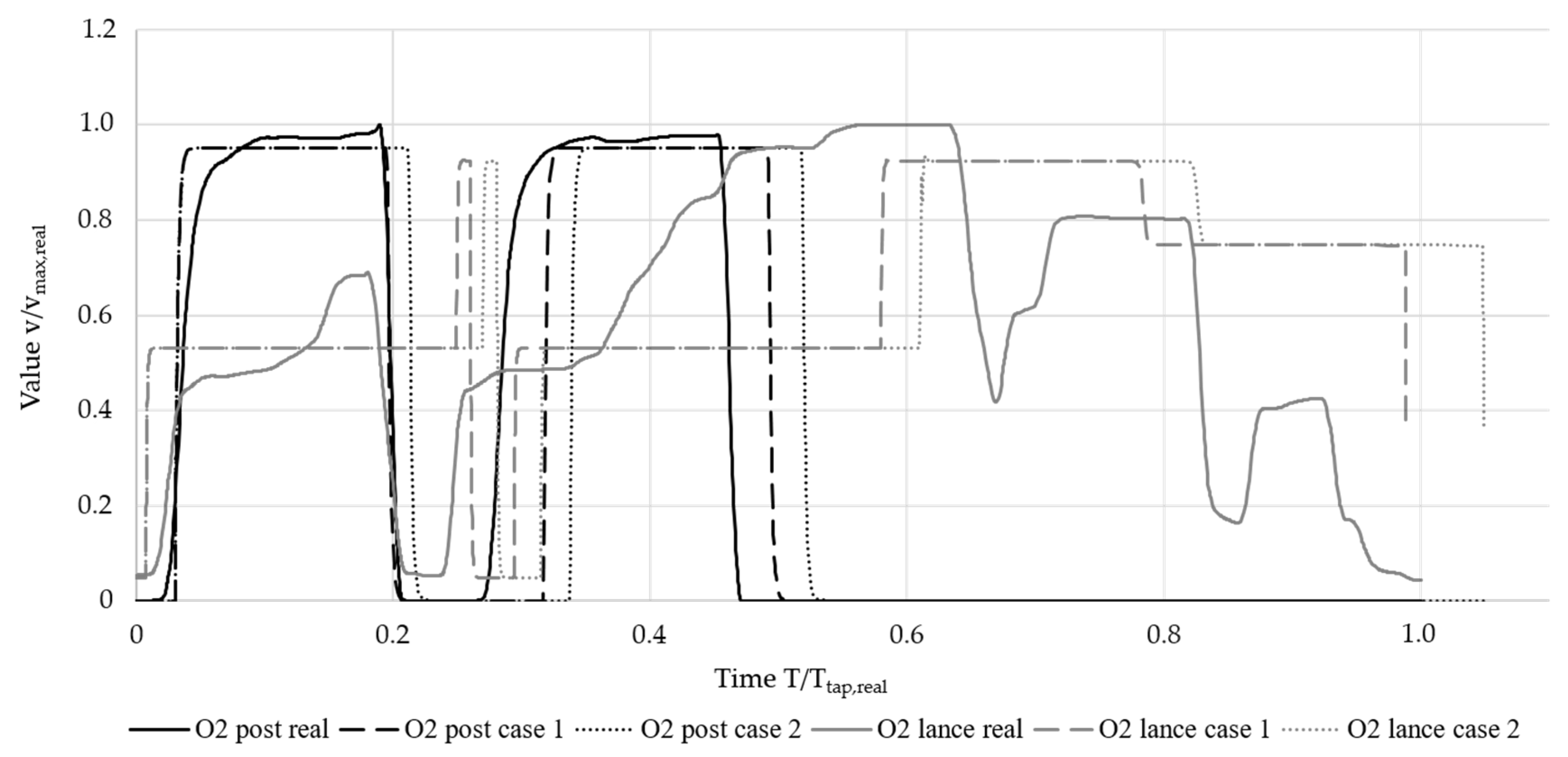
Figure 8 shows the normalized mass flows of post-combustion and lanced oxygen. The oxygen mass flow for natural gas combustion is not shown as its profile was similar to that of the natural gas shown in Figure 7. The post-combustion oxygen followed a profile comparable to that of the burners and showed good agreement with the measured values. With the automatic control, oxygen lancing was increased for a short period before the second basket was charged. At roughly 60% process time, the mass flow was increased to its maximum value and reduced again at around 80% for the flat bath phase until tapping. The measured value showed a smoother progression during meltdown and fluctuated more during the flat bath phase; however, the general profile and the total oxygen consumption could be reproduced during automatic control.
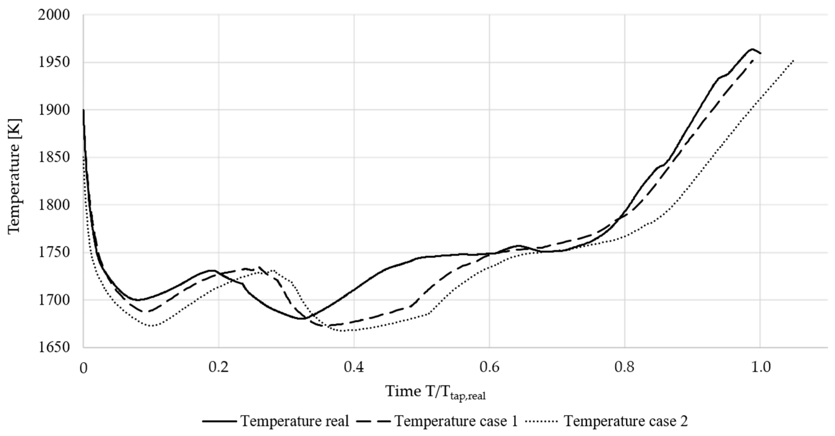
Figure 9 shows the progression of the simulated melt temperature for the measured operation chart and Cases 1 and 2. The delayed charging of the first basket was visible between 0.2 and 0.4 process time, as the temperature drop associated with the charging of cold scrap occurred later under automatic control. Although the temperature profile of Case 1 closely followed that of the measured case and reached tapping temperature almost simultaneously, the increased energy demand for Case 2 was visible in the lower temperature during the process and the delayed achievement of the desired tapping temperature. Overall, the automatic control implemented was able to reproduce the progression of the heat compared to the measured operation chart and indicate what impact a different oxygen source would have under otherwise similar conditions, showing the increased tap-to-tap time and consumption of electrical and chemical energy when the same operating strategies were applied in both cases.
Table 2 shows the resulting consumption of electric power, oxygen, natural gas, and coal, as well as the extracted off-gas and tap-to-tap time for the two cases relative to the values measured for the complete heat. Again, the increases in electrical and chemical energy used for Case 2 were visible.
5.2. Speed and Stability
For the simulator mode, the model speed and stability are most important. After charging a basket, the simulation is initiated and the solver takes 3–5 s to run the initial steps. After this initial delay, the simulator can be run at higher speed, allowing up to 20 seconds of the process to be simulated per second of real-time. Therefore, periods during meltdown or refining where no user input is necessary can be simulated at high speeds, whereas lower speeds can be selected during phases where frequent user inputs are necessary.
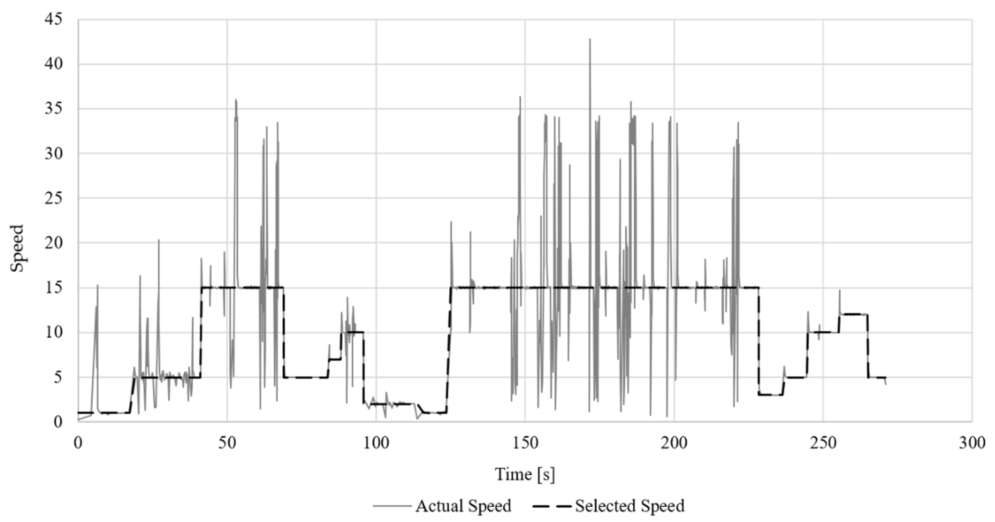
Figure 10 shows the progression of the selected simulation speed and the actual speed attained by the simulator during an example heat where two baskets were charged and a total process time of 2646 s was simulated in 272 s of real-time. The speed actually attained was calculated for each second of simulated process time. For most of the time, the simulation matched the selected speed; however, there were numerous instances where the speed dropped below the selected speed which was then compensated by an increased speed until the simulation and the target speed synchronized again. This never took more than a few seconds and the actual delay between the target time and the simulation stayed within less than 20 s. The short periods of re-synchronization were barely noticeable for the user, and inputs could be made precisely at the desired time and state of the simulated process.
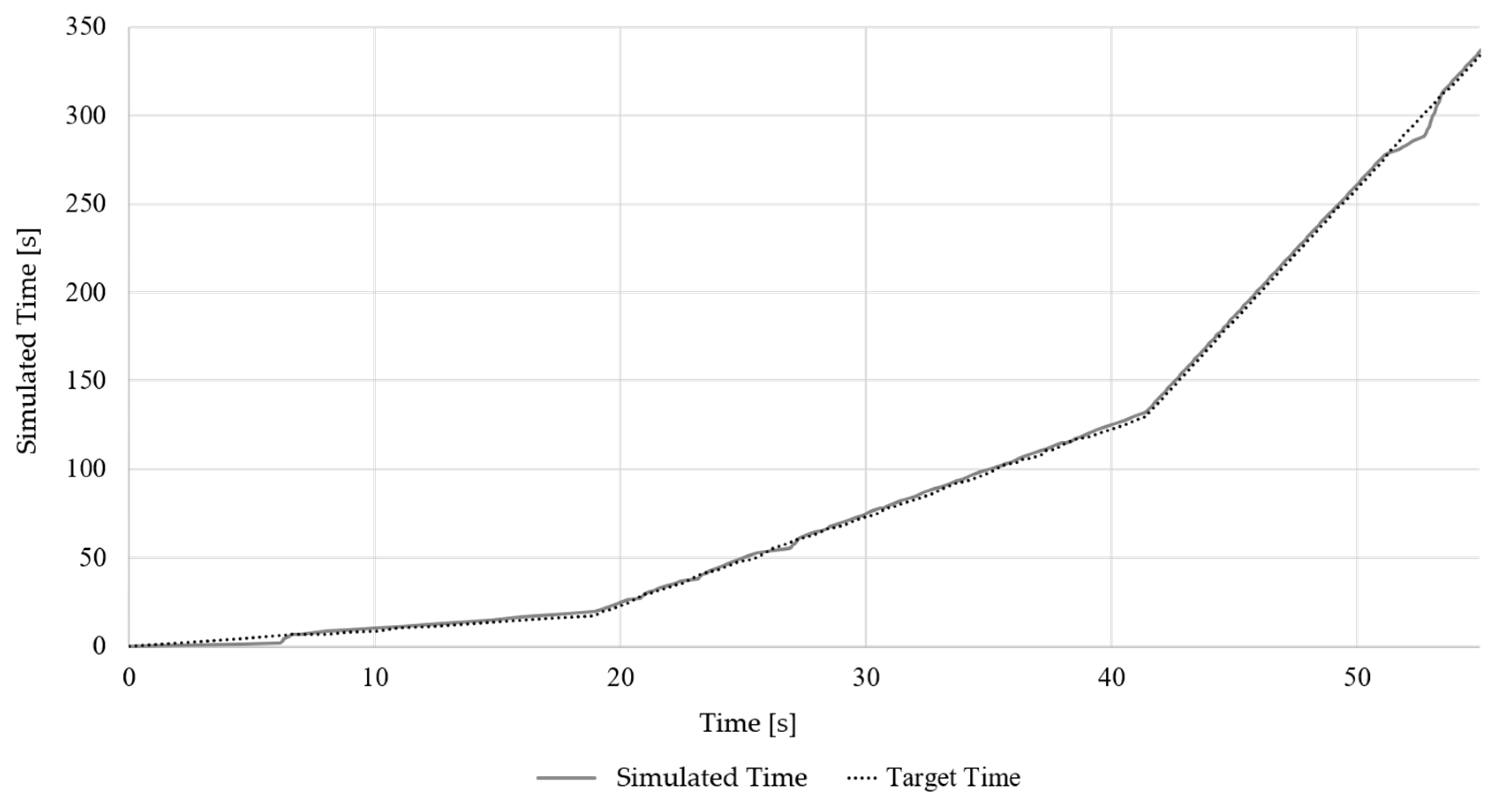
Figure 11 shows the simulated and the target time during the first 55 s of the same simulation. The delay during initialization is visible at 0–6 s, after which the simulation synchronized with the desired speed and closely matched the target time. After the initiation of the basket, deviations from the target time remained small and lasted for no more than 5 seconds.
Although results obtained with the automatic control and simulator cannot be validated using measured data, the internal consistency of the model can be evaluated using energy and mass balances. An energy balance using all heat flows calculated during the simulation yielded and error in the order of magnitude of 10−10 kWh, which was assumed to be a numerical error and was irrelevant for the simulation results. The mass balance prepared for each element gave a maximum error of 0.1% of the respective total mass, which was of no relevance for the simulation results.
The above examples illustrate the potential of the simulator developed. The simulator can be run in different modes depending on the aim of the simulation and, consequently, the simulator is applicable for different purposes such as process development, online predictions, and training of electric arc furnace operators. Simulators of this type are also applicable for dynamic optimization problems [40] and as soft sensors for evaluating parameters that are crucial for the EAF operators [3]. Another notion highlighting the importance of developing fundamental process models further is the fact that the computational load of comprehensive computational-fluid-dynamics-based approaches [41] remains—at least for the time being—too high for online applications.
5.3. Further Research
The Simulator mode allows direct user input and feedback during the simulation through a simple graphical interface. Although the current demonstrator is limited, all operation chart values can easily be added and manipulated during the simulation and additional settings such as compositions of charged materials for each basket could be added. All intermediate results of the model, such as temperatures, heat flows, and masses, are available during the simulation.
A target value is selected (for example 100 MW of electrical power) for both the automatic control and the simulator modes, and that exact value was used during the simulation, whereas in reality many operation chart values, especially the electrical power, current, and voltage, will fluctuate due to random influences such as the behavior of the electric arcs. In further work, a stochastic element could be added to introduce such fluctuations during simulations and produce more realistic behavior. Furthermore, it may be necessary to adjust the density of the scrap for each basket separately to better reproduce the behavior seen in real-life operation of the furnace.
In addition, further improvement of the underlying process model itself is of course possible. For example, a better representation of the melting behavior of scrap and adjustments for the use of other input materials, such as direct reduced iron, hot briquetted iron, or hot metal; improved description of the foaming of the slag; as well as the automatic adjustment of model parameters for different furnaces are possible areas of further research.
6. Conclusions
An automatic control and a simulator were developed on the basis of a comprehensive dynamic EAF process model that has previously been validated exhaustively using data from industrial furnaces. The automatic control is capable of reproducing real-live operation charts and adjusting them for different operating conditions. It can be used to evaluate various scenarios such as new control strategies, different materials for injection and charging, or the installation of new equipment. The rules currently used are partially based on parameters that cannot be measured or observed directly in the real-live process, and adjusted rules that are based more closely on the actual parameters used in process control such as total electric energy input and off-gas composition may be more useful for future work. The rules and parameters can be adjusted easily to allow different furnaces and operating strategies to be replicated and evaluated.
The simulator was shown to be stable and fast enough to run simulations based on user input in real-time as well as with higher speeds selected by the user with no noticeable delay apart from a few seconds during initialization after charging. Additional inputs and outputs can be added to make the simulator more versatile. For use in teaching and training, a more refined user interface and documentation would also be useful.
Due to the modular structure of the EAF process model simulations based on measured data, automatic control and simulator input can be run using the same basic model and structure with changes only necessary to the input module and the evaluation and output of the results, with the flexible solver algorithm allowing for stable and fast simulations for all cases. The model can therefore be used to evaluate the current state of the process and identify potential for improvement, to create and assess different scenarios and operating strategies, and for training and teaching using the simulator.
Author Contributions
Conceptualization, methodology, software, and writing—original draft preparation by T.H.; supervision, project administration, and writing—review and editing by T.E.; writing—review and editing by V.-V.V.
Funding
This research received no external funding
Conflicts of Interest
The authors declare no conflict of interest.
References
- Madias, J. Electric Furnace Steelmaking: Treatise in Process Metallurgy—Volume 3: Industrial Processes; Elsevier: Oxford, UK, 2014; pp. 271–300. [Google Scholar]
- Steel Statistical Yearbook 2018; World Steel Association: Brussels, Belgium, 2018.
- Logar, V.; Škrjanc, I. Development of an Electric Arc Furnace Simulator Considering Thermal, Chemical and Electrical Aspects. ISIJ Int. 2012, 52, 1924. [Google Scholar] [CrossRef]
- World Steel Association. Electric Arc Furnace Simulation. Available online: https://steeluniversity.org/product/electric-arc-furnace-simulation/ (accessed on 12 July 2019).
- Logar, V.; Škrjanc, I. Modeling and Validation of the Radiative Heat Tranfer in an Electric Arc Furnace. ISIJ Int. 2012, 52, 1225–1232. [Google Scholar] [CrossRef]
- Logar, V.; Dovžan, D.; Škrjanc, I. Modeling and Validation of an Electric Arc Furnace Part 1, Heat and Mass Transfer. ISIJ Int. 2012, 52, 402–412. [Google Scholar] [CrossRef]
- Logar, V.; Dovžan, D.; Škrjanc, I. Modeling and Validation of an Electric Arc Furnace Part 2, Thermo-chemistry. ISIJ Int. 2012, 52, 413–423. [Google Scholar] [CrossRef]
- Logar, V.; Dovžan, D.; Škrjanc, I. Mathematical modeling and experimental validation of an electric arc furnace. ISIJ Int. 2011, 51, 382–391. [Google Scholar] [CrossRef]
- Electric Arc Furnace Simulation User Guide; University of Liverpool: Liverpool, UK, 2006.
- Bekker, J.G.; Craig, I.K.; Pistorius, P.C. Model predictive control of an electric arc furnace off-gas process. Control Eng. Pract. 2000, 8, 445–455. [Google Scholar] [CrossRef]
- Bekker, J.G.; Craig, I.K.; Pistorius, P.C. Modeling and Simulation of an Electric Arc Furnace Process. ISIJ Int. 1999, 39, 23–32. [Google Scholar] [CrossRef]
- Bekker, J.G. Modelling and Control of an Electric Arc Furnace Off-Gas Process. Master’s Thesis, University of Pretoria, Pretoria, South Africa, 1998. [Google Scholar]
- MacRosty, R.D.M.; Swartz, C.L.E. Dynamic optimization of electric arc furnace operation. AIChE J. 2007, 53, 640–653. [Google Scholar] [CrossRef]
- MacRosty, R.D.M.; Swartz, C.L.E. Dynamic modeling of an industrial electric arc furnace. Ind. Eng. Chem. Res. 2005, 44, 8067–8083. [Google Scholar] [CrossRef]
- MacRosty, R.D.M.; Swartz, C.L.E. Optimization as a tool for process improvement in EAF operations. In Proceedings of the Iron and Steel Technology Conference AISTech, Charlotte, NC, USA, 9–12 May 2005. [Google Scholar]
- Matson, S.; Ramirez, W.F. Optimal Operation of an Electric Arc Furnace. In Proceedings of the 57th Electric Furnace Conference, Pittburgh, PA, USA, 14–16 November 1999. [Google Scholar]
- Matson, S.A.; Ramirez, W.F. The dynamic modeling of the electric arc furnace. In Proceedings of the 55th Electric Furnace Conference, Chicago, IL, USA, 9–12 November 1997. [Google Scholar]
- Matson, S.A.; Ramirez, W.F.; Safe, P. Modeling an EAF using Dynamic Material and Energy Balances. In Proceedings of the 56th Electric Furnace Conference, New Orleans, LA, USA, 15–18 November 1998. [Google Scholar]
- Deneys, A.C.; Peaslee, K.D. Post-Combustion in the EAF—A Steady State Simulation Model. In Proceedings of the 55th Electric Furnace Conference, Chicago, IL, USA, 9–12 November 1997. [Google Scholar]
- Shah, D.H.; Peaslee, K.D. Post Combustion in EAF-Dynamic Simulation Model. In Proceedings of the 56th Electric Furnace Conference, New Orleans, LA, USA, 15–18 November 1998. [Google Scholar]
- Cameron, A.; Saxena, N.; Broome, K. Optimizing EAF Operations by Dynamic Process Simulation. In Proceedings of the 56th Electric Furnace Conference, New Orleans, LA, USA, 15–18 November 1998. [Google Scholar]
- Cameron, A. Optimising electric arc furnace operations. Steel Times 1999, 227, 7–10. [Google Scholar]
- Modigell, M.; Traebert, A.; Monheim, P. A modelling technique for metallurgical processes and its applications. AISE Steel Technol. 2001, 78, 45–47. [Google Scholar]
- Traebert, A.; Modigell, M.; Monheim, P.; Hack, K. Development of a modelling technique for non-equilibrium metallurgical processes. Scand. J. Metall. 1999, 28, 285–290. [Google Scholar]
- Morales, R.D.; Rodríguez-Hernández, H.; Conejo, A.N. A mathematical simulator for the EAF steelmaking process using direct reduced iron. ISIJ Int. 2001, 41, 426–436. [Google Scholar] [CrossRef]
- Nyssen, P.; Colin, R.; Knoops, S.; Junque, J. On-line EAF control with a dynamic metallurgical model. In Proceedings of the 7th European Electric Steelmaking Conference (EEC), Venice, Italy, 26–29 May 2002. [Google Scholar]
- Nyssen, P.; Marique, C.; Prüm, C.; Bintner, P.; Savini, L. A New Metallurgical Model for the Control of EAF Operations. In Proceedings of the 6th European Electric Steelmaking Conference, Düsseldorf, Germany, 13–15 June 1999. [Google Scholar]
- Nyssen, P.; Monfort, G.; Junque, J.L.; Brimmeyer, M.; Hubsch, P.; Baumert, J.C. Use of a dynamic metallurgical model for the on-line control and optimization of the electric arc furnace. In Proceedings of the STEELSIM, 2nd International Conference of Simulation and Modelling of Metallurgical Processes in Steelmaking, Graz/Seggau, Austria, 12–14 September 2007. [Google Scholar]
- Nyssen, P.; Ojeda, C.; Baumert, J.C.; Picco, M.; Thibaut, J.C.; Sun, S.; Waterfall, S.; Ranger, M.; Lowry, M. Implementation and on-line use of a dynamic process model at the ArcelorMittal-Dofasco electric arc furnace. In Proceedings of the STEELSIM, 4th International Conference of Simulation and Modelling of Metallurgical Processes in Steelmaking, METEC InSteelCon, Düsseldorf, Germany, 27 June–1 July 2011. [Google Scholar]
- Arnout, S.; Verhaeghe, F.; Blanpain, B.; Wollants, P.; Hendrickx, R.; Heylen, G. A Thermodynamic Model of the EAF Process for Stainless Steel. Steel Res. Int. 2006, 77, 317–323. [Google Scholar] [CrossRef]
- Kho, T.S.; Swinbourne, D.R.; Blanpain, B.; Arnout, S.; Langberg, D. Understanding stainless steelmaking through computational thermodynamics Part 1: Electric arc furnace melting. Trans. Inst. Min. Metall. Sect. C 2010, 119, 1–8. [Google Scholar] [CrossRef]
- Meier, T.; Gandt, K.; Hay, T.; Echterhof, T. Process Modeling and Simulation of the Radiation in the Electric Arc Furnace. Steel Res. Int. 2018, 89, 1700487. [Google Scholar] [CrossRef]
- Meier, T.; Hay, T.; Echterhof, T.; Pfeifer, H.; Rekersdrees, T.; Schlinge, L.; Elsabagh, S.; Schliephake, H. Process Modeling and Simulation of Biochar Usage in an Electric Arc Furnace as a Substitute for Fossil Coal. Steel Res. Int. 2017, 88, 1600458. [Google Scholar] [CrossRef]
- Meier, T.; Gandt, K.; Echterhof, T.; Pfeifer, H. Modeling and Simulation of the Off-gas in an Electric Arc Furnace. Metall. Mater. Trans. B 2017, 48, 3329–3344. [Google Scholar] [CrossRef]
- Meier, T. Energetische Analyse des Sauerstoffeinsatzes im Elektrolichtbogenofen Mithilfe Eines Selbstregelnden Dynamischen Prozessmodells. Master’s Thesis, RWTH Aachen University, Aachen, Germany, 2017. [Google Scholar]
- Meier, T.; Logar, V.; Echterhof, T.; Igor, Š.; Pfeifer, H. Modelling and Simulation of the Melting Process in Electric Arc Furnaces—Influence of Numerical Solution Methods. Steel Res. Int. 2016, 87, 581–588. [Google Scholar] [CrossRef]
- Meier, T. Modellierung und Simulation des Elektrolichtbogenofens. Ph.D. Thesis, RWTH Aachen University, Aachen, Germany, 2016. [Google Scholar]
- Fathi, A.; Saboohi, Y.; Škrjanc, I.; Logar, V. Comprehensive Electric Arc Furnace Model for Simulation Purposes and Model-Based Control. Steel Res. Int. 2017, 83, 1600083. [Google Scholar] [CrossRef]
- Hay, T.; Reimann, A.; Echterhof, T. Improving the Modeling of Slag and Steel Bath Chemistry in an Electric Arc Furnace Process Model. Metall. Mater. Trans. B 2019, 50, 2377–2388. [Google Scholar] [CrossRef]
- Saboohi, Y.; Fathi, A.; Škrjanc, I.; Logar, V. Optimization of the Electric Arc Furnace Process. IEEE Trans. Ind. Electron. 2019, 66, 8030–8039. [Google Scholar] [CrossRef]
- Odenthal, H.-J.; Kemminger, A.; Krause, F.; Vogl, N. A Holistic CFD Approach for Standard and Shaft-Type Electric Arc Furnaces. In Proceedings of the AISTech 2017, Nashville, TN, USA, 8–11 May 2017. [Google Scholar]
Figure 1.
Model zones.

Figure 2.
Model structure (translated from [37]). EAF: electric arc furnace.
Figure 2.
Model structure (translated from [37]). EAF: electric arc furnace.

Figure 3.
Data module with measured data.

Figure 4.
Data module for automatic control and simulator modes.

Figure 5.
User interface.

Figure 6.
Electric power comparison.

Figure 7.
Natural gas and injected coal comparison.

Figure 8.
Oxygen comparison.

Figure 9.
Melt temperature comparison.

Figure 10.
Selected and attained simulation speed.

Figure 11.
Simulated and target time.


Table 1.
Parameters for automatic control.
| Parameter | Unit | Description |
|---|---|---|
| tstop-delay | s | Time to raise electrodes and open roof |
| tstart-delay | s | Time to close roof and lower electrodes |
| Vscrap-max | % | Maximum fraction of furnace volume that can be filled with scrap |
| Pstart-reduction | % | Reduction of electric power during bore down (until arc is covered by scrap) |
| Prefine-reduction | % | Reduction of electric power during refining (flat bath) |
| Pwall-reduction | % | Reduction of electric power when water-cooled wall overheats |
| Twall-crit | K | Critical wall temperature for power reduction |
| Olance-min | % | Fraction of maximum value during reduced lancing |
| Clance-burner | % | Oxygen lancing increased when burner power below this fraction |
| Clance-bath | % | Influence of free bath surface on oxygen lancing |
| Cpost-scrap | % | Post-combustion reduced when remaining scrap below this fraction |
| tpost-delay | s | Post-combustion starting with delay after power on |
| Cburner-scrap | % | Burner power reduced when remaining scrap below this fraction |
| Ccarbon-batth | % | Carbon lancing initiated when free bath surface above this fraction |
| Ccarbon-scrap | % | Carbon lancing reduced when remaining scrap below this fraction |
Table 2.
Calculated performance indicators for the study cases.
| Parameter | Case 1 | Case 2 |
|---|---|---|
| Electric energy | 1 | 1.06 |
| Oxygen through lance | 1.1 | 1.17 |
| Oxygen for post-combustion | 1 | 1.06 |
| Injected carbon | 0.9 | 0.96 |
| Off-gas | 1.06 | 1.13 |
| Natural gas | 0.99 | 1.04 |
| Oxygen for natural gas burners | 1 | 1.07 |
| Total oxygen | 1.07 | 1.14 |
© 2019 by the authors. Licensee MDPI, Basel, Switzerland. This article is an open access article distributed under the terms and conditions of the Creative Commons Attribution (CC BY) license (http://creativecommons.org/licenses/by/4.0/).
Share and Cite
MDPI and ACS Style
Hay, T.; Echterhof, T.; Visuri, V.-V. Development of an Electric Arc Furnace Simulator Based on a Comprehensive Dynamic Process Model. Processes 2019, 7, 852. https://doi.org/10.3390/pr7110852
AMA Style
Hay T, Echterhof T, Visuri V-V. Development of an Electric Arc Furnace Simulator Based on a Comprehensive Dynamic Process Model. Processes. 2019; 7(11):852. https://doi.org/10.3390/pr7110852
Chicago/Turabian StyleHay, Thomas, Thomas Echterhof, and Ville-Valtteri Visuri. 2019. "Development of an Electric Arc Furnace Simulator Based on a Comprehensive Dynamic Process Model" Processes 7, no. 11: 852. https://doi.org/10.3390/pr7110852
Note that from the first issue of 2016, this journal uses article numbers instead of page numbers. See further details here.