


Robust Placement and Control of Phase-Shifting Transformers Considering Redispatch Measures


Energy Information Networks & Systems, Technical University of Darmstadt, 64283 Darmstadt, Germany
*
Author to whom correspondence should be addressed.
Energies 2023, 16(11), 4438; https://doi.org/10.3390/en16114438
Submission received: 19 April 2023
/
Revised: 23 May 2023
/
Accepted: 26 May 2023
/
Published: 31 May 2023
(This article belongs to the Special Issue Optimal Power Flow: Optimization and Control of Electric Power Systems)
Abstract
:Flexible AC transmission systems (FACTSs) can maximize capacity utilization under time-varying grid usage patterns by actively controlling the power flow of the transmission lines, e.g., with phase-shifting transformers (PST). In this paper, we propose an algorithm to determine the minimum number of PSTs and their location such that the grid can operate robustly for any realization of the (active) power set points from a known, continuous uncertainty set. As we show in our experiments, only considering a few extreme grid scenarios cannot provide this guarantee. The proposed algorithm considers the trade-offs between PST placement and operational decisions, such as PST control and redispatch. By minimizing the worst-case redispatch cost, it yields two affine linear control policies for these as a byproduct. Power flow is modeled as a constrained linear system, and the control design and actuator minimization tasks are formulated as a mixed-integer linear program (MILP). We also design a greedy algorithm, whose optimal value differs less than 20% from the MILP solution while being one to two orders of magnitude faster to compute. The proposed algorithm is evaluated for a small demonstrative 3-bus example and the IEEE 39 bus test system.
1. Introduction
Variable renewable energies from wind and sun are important to reduce the global carbon footprint of energy systems. At the same time, their variability creates novel challenges for both the design and the operation of transmission grids. Especially when large renewables capacities are localized in few regions with good natural resources, their power generation may lead to line overloads in the grid. Redispatch is a common measure to counteract these congestions, but it may be expensive. Grid capacity extensions are a last resort but typically require a long time to implement and are subject to societal resistances. Thus, utilizing active power flow control technologies in the grid is an attractive and often cost-effective option for grid operators. Flexible alternating current transmission systems (FACTSs) utilize power electronics to enhance the grid’s controllability [1]. Examples include static var compensators (SVC), thyristor-controlled series capacitors (TCSCs), and thyristor-controlled phase-shifting transformers (PST), which are part of various grid development plans, e.g., in Germany (www.netzentwicklungsplan.de (accessed on 2 February 2023)).
An important question that naturally arises is where to place such FACTS devices in the power grid and how to control them. Maximizing the loadability of the system for one demand scenario considering various FACTS devices can be solved by genetic algorithms [2] or by the alternating direction method of multiplier (ADMM) [3]. Mixed integer linear programming (MILP) can be used for PST [4] or SVC [5] placement in the same one-scenario setting. Several scenarios are considered in approaches based on two-stage stochastic programming [6,7,8], which allows to account for the expected scenario-dependent generation costs as well. All of these approaches do not guarantee system feasibility or the (re-)dispatch costs for situations outside the (typically few) considered scenarios. In our experimental section, we show that relying only on extreme generation situations may be misleading about the grid’s feasibility for intermediate in-feeds.
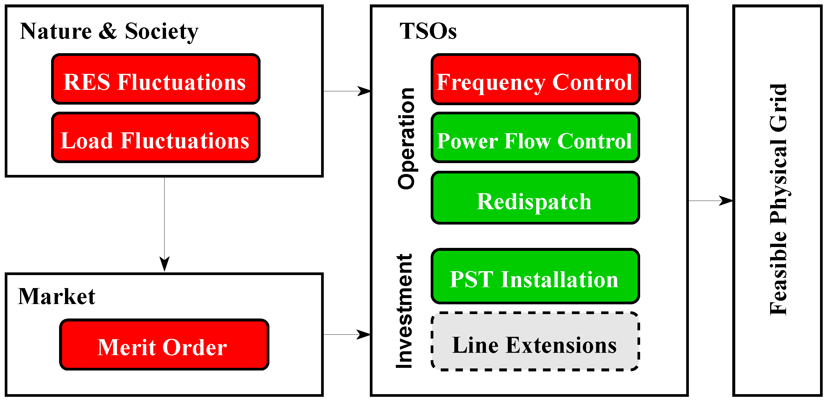
In this paper, we propose an algorithm to find the minimal number and location of PSTs that can guarantee system feasibility and limit redispatch costs for all scenarios in a continuous uncertainty set. Considered uncertainty factors are renewable, and load fluctuations as well as the corresponding dispatch decisions are determined by markets or load–frequency control, see Figure 1. During PST placement, we take into account the grid operators’ situation-dependent control options, such as specifying PST settings and redispatch orders to the attached power plants. Our algorithm thus produces, as a byproduct of the PST placement task, control policies to dynamically determine the PST settings and the redispatch orders. These policies are assumed to be affine linear in the uncertain factors in our work. They are chosen optimally in the sense that they minimize the worst-case redispatch cost in this class of controls. Since we consider the often strongly non-linear dispatch decisions by markets and frequency control as part of the uncertainty set, the linearity assumption for small to medium-sized redispatch corrections is plausible.
In our proposed method, we model the power flow in the grid as a set of linear equations, similar to the approach used in [9,10]. However, we employ a robust optimization framework instead of relying on chance constraints to model the uncertainty in power injections. Doing so allows us to write the continuous part of the placement and control problem as a linear program, which is easier to solve than the second-order cone programs derived from chance-constrained optimization problems. The authors of [11] also use a robust optimization approach in the context of reserve scheduling in power systems with highly uncertain power injections. In our work, we extend this approach by also considering the optimal location of PSTs. The resulting robust optimization problem can be solved with MILP. It is worth noting that fuzzy logic represents a widely used alternative to handle uncertainty in power systems [12,13,14]. However, fuzzy methods may encounter scalability issues when dealing with the large-scale problems often encountered in power systems. Consequently, heuristics may be necessary to reduce solving times [15].
The uncertainty set considered in the robust optimization should be large enough to cover at least a selection of plausible scenarios and all mixtures of these. At the same time, the uncertainty set should not be too large in order to avoid excessive conservatism of the solution. We use principal component analysis (PCA) [16] based on a set of given scenarios to define the uncertainty set as a rotated hyperrectangle as in [17]. While the solution might be conservative, it is guaranteed to yield feasible system states for this continuous set.
Due to the computational expense of exact methods to determine the optimal placement of FACTS, various studies have suggested heuristics as a solution to this problem [18,19,20]. In this study, we also propose a greedy algorithm that yields near-optimal solutions while being much faster to solve than the MILP. It iteratively checks for improvement in the objective function when adding a PST to a transmission line in a hill-climbing fashion. In each iteration, the algorithm solves the linear programming relaxation of the proposed MILP and projects the fractional solution onto the feasible set of the original problem. While the maximum number of iterations grows linearly with the number of transmission lines in the grid, a parametrized stopping condition can drastically reduce the algorithm’s search space. We demonstrate that for a realistically sized transmission grid, the greedy algorithm is more than 40 times faster to compute than the MILP and finds a solution with an objective value that is 17% greater. Despite a relatively big optimality gap for a planning problem, the solution of the greedy algorithm is still useful, e.g., in preliminary grid analyses.
Two examples are evaluated numerically. The first example with three buses stylizes a typical grid situation in Germany, where centralized wind power leads to loop flows through neighboring countries. The computed affine linear policies are compared against optimizing the redispatch separately for each scenario. We can show that considering only extreme scenarios with no or maximal wind generation are not sufficient to guarantee grid feasibility in all situations. The second example uses the IEEE 39 bus test case and real-world time series.
The remainder of the paper is structured as follows. In Section 2, we define the linear power flow model employed throughout this work. We give a formal problem definition in Section 3. Section 4 presents our proposed MILP formulation assuming that the uncertainty set is a (convex) polytope. In Section 5, we show how to construct the polytopic uncertainty set given a collection of renewable and load scenarios and their corresponding dispatch results. The numeric evaluation is described in Section 7. Conclusions are drawn in Section 8.
2. Power Flow Model
We use the common DC approximation [21] to linearly model the power flow in a transmission grid with N buses and L lines. Power line flows are denoted as , voltage phase angles as , and the phase shifts potentially added by the PSTs as . We then have
where is the grid’s incidence matrix and is a diagonal matrix with the line susceptances.
Let be the uncertain vector of power set points of the P generators/loads of the grid, where is the corresponding uncertainty set. Moreover, let denote the vector of power adjustments caused by redispatch actions. The power injections at the buses of the grid are then given by
where is the matrix that maps generators/loads to the buses, at which they are connected to the grid. According to Kirchhoff’s first law, the nodal power injections match the sum of the power flows on the connected lines, i.e., . By substituting (1) into the previous relationship and equalizing it with (2), it is possible to express the voltage phase angles of the buses as
Since a constant shift of the phase angles does not change the physical situation, is not invertible, and we use the pseudo-inverse to obtain a minimum norm solution. Substituting (3) into (1), the power line flows can be written as a linear function of the power set points , the redispatch and the phase shifts added by the PSTs as
with . Throughout this paper, denotes the identity matrix with appropriate dimensions. This model allows us to express line capacity constraints as a linear function of the modeled uncertainties and the control decisions.
3. Formal Problem Statement
The optimization of the number and placement of PSTs needs to consider the control actions to be performed with them as well as the effect of redispatch measures that are important additional operational measures available to the grid operators. In this paper, we assume that the control policies for setting the phase shifts and the power adjustments are affine linear functions of the system state, i.e., they depend linearly on the uncertain power set points . We, thus, can write the policies as
where is parametrized by and , and by and .
We now can formally define the optimization task we aim to solve in this work. We aim at determining the minimal set of PSTs and their location along with the control policies (5) and (6) such that the total worst-case redispatch costs and the PST installations costs are minimized while ensuring that the grid operates within its feasible region for any realization of the uncertain elements . With indicating the placement of a PST at a transmission line and being the worst-case redispatch cost, the optimization problem can then be written as
Here, is a vector of ones with appropriate dimensions, and is a weighting factor between the cost for placing the PSTs in the grid and the worst-case redispatch cost. It should be chosen depending on the assumed probability of the worst-case redispatch situation. Vector denotes the maximum transport capacity of the lines, and is the PST technical constraint on the maximum allowed phase shift. Redispatch power adjustments sum to zero and should not violate the situation-dependent physical limitations , of generation or consumption for each element of . An example of such bounds is and for wind and solar power plants. We generally assume a linear relation, i.e., and , where and are diagonal matrices. Moreover, represents the cost of increasing the power output of a generator/load by one unit.
4. Robust Optimization with Polytopic Uncertainty
In this section, we formulate a MILP model to solve the optimization task defined in the last section. By assuming a polytopic uncertainty set , we are able to express the infinite number of robustness constraints as a finite set of linear constraints using duality properties.
To this end, we first use expression (4) and the parametrizations (5) and (6) to rewrite the constraints of (7) in compact matricial form, i.e.,
with and being defined in (9) and (10), respectively, where · represents zero entries:
Next, we assume that the uncertainty set of the power set points is a polytope defined as the intersection of M halfspaces. That is, given the exterior representation of
with and , we assume that such that , . In our experiments, the uncertainty set is guaranteed to be a polytope by construction as shown in Section 5.
Using (8) and (11), our optimization task is equivalent to the following min-max optimization problem:
where K is the number of rows of , is the set , is the j-th row of , and is the j-th element of .
We transform the min-max problem (12) into a single-stage linear program using duality theory. As is nonempty and bounded, the inner optimization problem is always feasible, and hence its primal and dual problems have the same objective value by strong duality. We can thus rewrite (12) as
where are the dual variables of the j-th inner problem. Optimization problem (13) can then be formulated as a single-level minimization problem:
The equivalence between (13) and (14) can be verified by noticing that an optimal solution for (14) is also a feasible solution for (13) and that both objective functions have the same value. On the other hand, an optimal solution for the outer problem of (13) implies that there exists a that satisfies the constraints of the inner problem, and, thus, the solution would also be feasible in (14), and both objective functions would have the same value.
5. Robust Uncertainty Set
The optimization formulated above enables us to solve the robust PST placement problem as a MILP model given a polytopic uncertainty set . As sketched in Figure 1, the influencing factors to be described via the uncertainty set are not only the renewable and load uncertainties but also the market and frequency control measures. These potentially large effects are determined via complex mechanisms, often showing highly non-linear behavior with respec to the loads and renewables. For example, the classic merit-order algorithm uses one power plant after the other in full, but it does not proportionally scale production levels. By including these factors in the uncertainty set, the linearity assumption for the remaining minor deviations from redispatch and active flow control can be justified.
To create realistic uncertainty sets, we propose to generate samples by creating a set of plausible renewable generation and load scenarios either from measurements or probabilistic models. For each scenario a market model, e.g., a simple merit-order dispatch, is used to compute the dispatch decisions. The full information is then used to generate a continuous uncertainty set that covers the modeled scenarios but also the space in between, i.e., all (convex) combinations of them.
Given S scenarios of the uncertain vector of power set points , , a first set enclosing all these points can be defined as
where and are defined as and for all dimensions .
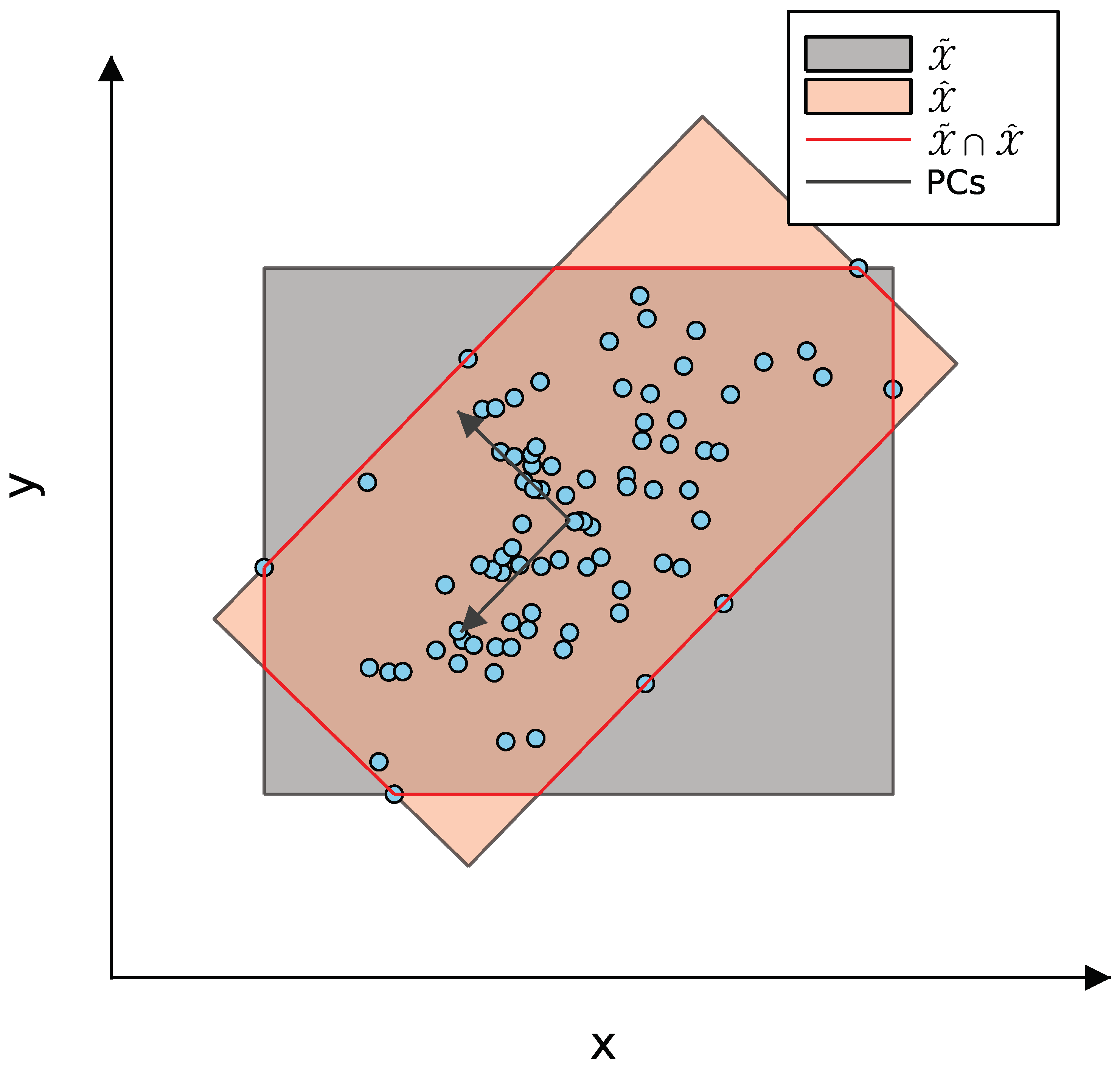
However, as shown in Figure 2, this axis-aligned hyperrectangle can be large and lead to overly conservative solutions in case the components of are highly correlated, which is usually the case in power systems (consider, for instance, that the wind or photovoltaic production in close by locations will typically be similar).
To leverage these correlations between the different dimensions of the scenarios, we use PCA to compute a tighter, rotated uncertainty set as in [17].
Let be the data matrix. We first center the data by subtracting them by their empirical mean to obtain the matrix . Next, we calculate the empirical covariance matrix as . Symmetric matrix can be diagonalized, i.e., , where has the eigenvectors of in its columns and is a diagonal matrix with the corresponding eigenvalues on its diagonal. This allows us to construct a rotated, data-aligned hyperrectangle as
where and , with and being the j-th elements of the row vectors and containing the maximum and minimum values among the S scenarios in the direction of the principal components, respectively.
With this approach, we are able to fit a possibly much tighter set to the scenarios by defining the uncertainty set as the intersection between and , i.e.,
which is shown in Figure 2.
6. Greedy Algorithm for Solving Robust MILP
As the size of the grid increases, the runtime for solving (14) to optimality becomes too long as shown in our experiments (see Section 7). We, thus, propose a hill-climbing-like heuristic that iteratively checks whether adding a PST to a line decreases the value of the objective function. Each iteration relies on solving the linear programming relaxation of (14) and projecting the fractional solution onto the feasibility set of the original MILP. The algorithm performs, at most, L iterations, thus yielding polynomial time complexity. However, the solution of the proposed method is only guaranteed to be a local minimum on the solution space of the original MILP by nature of the hill-climbing procedure.
The algorithm first determines a lower bound for the objective function of (14) by solving its linear programming relaxation, as any solution of the (mixed-)integer program is a feasible solution of its linear relaxation. If the optimal solution of the relaxed problem has all values of as 0 or 1, it will also be the optimal solution to the MILP. To obtain an upper bound, we can solve (14) with fixed to the value of the solution to the relaxed problem rounded to the closest integer.
The algorithm proceeds in a hill-climbing fashion to improve the integer solution. With being the value of from the solution to the relaxed problem, the algorithm places a PST into the line corresponding to the largest element of , i.e., it fixes element of to 1. If the line already has a PST, the algorithm adds a PST to the line corresponding to the next largest element of . With one of the elements of fixed, the algorithm solves the relaxed problem and uses the rounded solution to update the upper bound of the objective function. The algorithm continues adding PSTs to the grid until the value of the objective function stops decreasing between iterations, or if the largest element of is smaller than some parameter .
The pseudocode for the proposed greedy algorithm is presented in Algorithm 1, where ⌀ is the empty set, is the set of lines with PST, is the round operator, and represents the cardinality of a set. While the Main procedure implements the hill-climbing algorithm, the solve procedure solves the linear relaxation of the original MILP (14) with the variables corresponding to the lines that are already equipped with PST being fixed to one.
| Algorithm 1 Greedy algorithm for solving robust MILP. |
|
7. Experiments
We demonstrate our proposed approach for two examples, a small 3-bus test grid and the IEEE 39 bus system. Our implementation uses the modeling language JuMP [22] and Gurobi [23] to solve the MILP model (14).
7.1. 3-Bus Test Grid
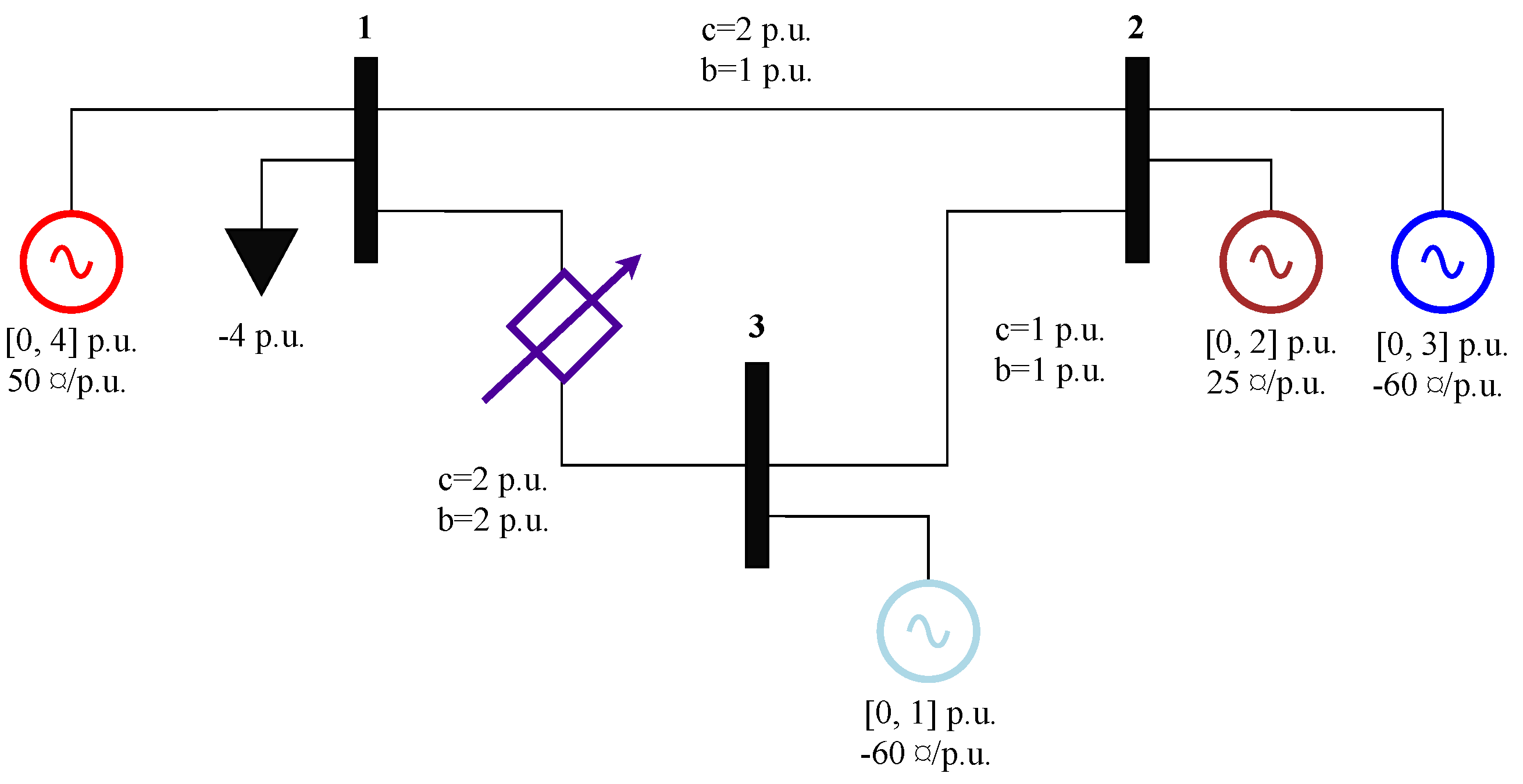
We first apply the proposed algorithm to the grid in Figure 3. The figure also contains the values of the loads, generator limits and unit costs, as well as line capacities and susceptances. The unit cost of wind production has a negative value, mirroring precedence for renewable power generation over conventional one, as well as standard subsidy policies.
Power is represented in the per unit system (p.u.) for some base power value and costs in a generic currency ¤. The example is a stylized sketch of the situation in Germany, with much wind and lignite generation in the East and the load center and many gas power plants in the Southwest [24]. Bus 3 would then represent neighboring countries.
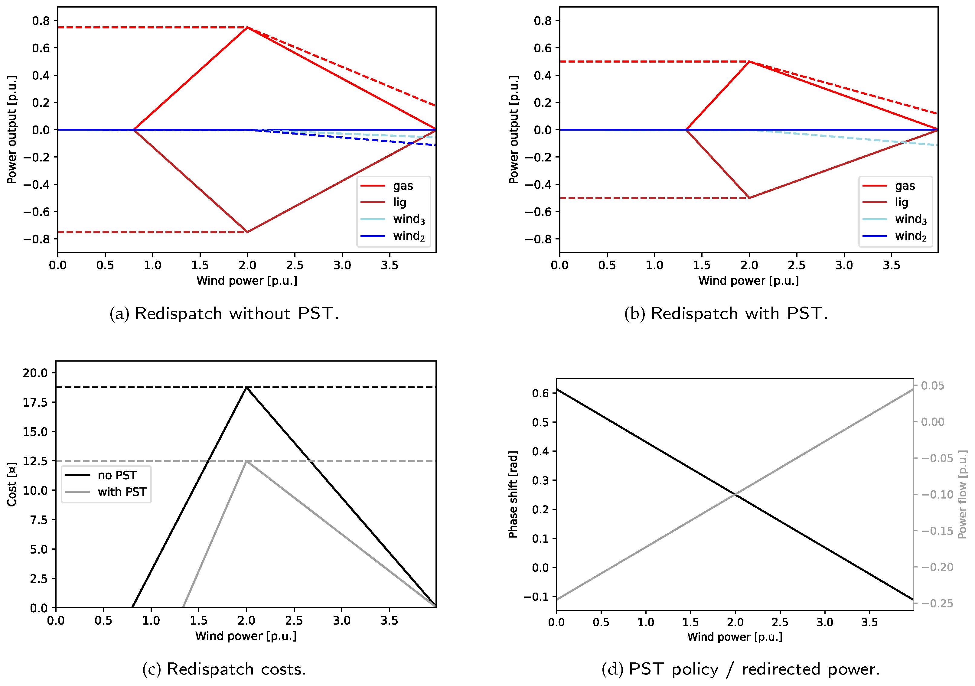
In Figure 4, we examine the operation patterns of the test grid when varying the available wind power from zero to its maximum capacity. Both wind sites are scaled proportionally. For each wind in-feed, we determine the cost optimal dispatch using the merit order algorithm. Demands that cannot be covered from wind alone are supplied by the lignite power plant first and then by the gas power plant. For each scenario, we then obtain a cost-optimal redispatch by solving (7).
As can be seen in Figure 4, no redispatch is needed when the wind is minimal or maximal: the merit-order dispatch is directly feasible. With no wind, the generation pattern is 2 p.u. at bus 1 and 2 p.u. at bus 2. With maximum wind, the generation is 3 p.u. at bus 2 and 1 p.u. at bus 3. A grid analysis based only on these two scenarios could conclude that the grid can be feasibly operated for all possible wind outputs without additional measures, such as PST placement or redispatch. However, this would be the wrong conclusion, since for 2 p.u. of wind, the generation pattern is 3.5 p.u. at bus 2 and 0.5 p.u. at bus 3, which leads to a capacity violation on line (2,3). This example thus proves that relying on few scenarios, as is often done for two-stage stochastic programming approaches due to computational limitations, is not enough to ensure universal grid feasibility. In contrast, our robust approach considers a continuous uncertainty with all (convex) scenario mixtures included. While for this low-dimensional example, one can obviously include average scenarios into a scenario-based analysis, this would be much more difficult in more complex, high-dimensional setups, where the number of required scenarios could be huge. Note that our approach scales only in the dimension of the uncertainties but not in the number of scenarios, which can grow exponentially with the number of uncertainty dimensions if an even cover of the scenario space is desired.
In Figure 4a,b, we also show the redispatch policies computed by solving (14). For Figure 4a, we choose such that no PST is installed, but higher redispatch costs are preferable, whereas in Figure 4b, the parameter is chosen to be small enough such that one PST on line (1,3) is optimal. Note that the derived values of the computed redispatch policy are not linear in the wind power production. However, they are affine linear in the dispatch, including the non-linear merit order results. Even for this low-dimensional example, the redispatch policies qualitatively resemble the optimal redispatch values computed for each scenario individually. For higher-dimensional examples, the linearity condition might even be less restrictive. For both cases, with and without PST, the implied worst-case cost by the computed affine linear policy matches the worst-case cost of the scenario-wise optimized redispatch schedule as shown in Figure 4c.
The example also shows that the redispatch cost can be reduced by increasing the controllability of the power flow in the grid with the addition of a PST. Figure 4d shows the angle shift added by the PST following the affine control policy as well as the amount of power flow redirected from branch (2,3) to (2,1). These settings ensure a feasible grid power flow in all situations. It is worth noting that in the “no wind” situation, the PST also redirects energy from line (2,3) to line (1,2), which helps increase the distance to the feasibility border since without PST interaction the line (2,3) would be fully loaded.
7.2. IEEE 39 Bus Test Case
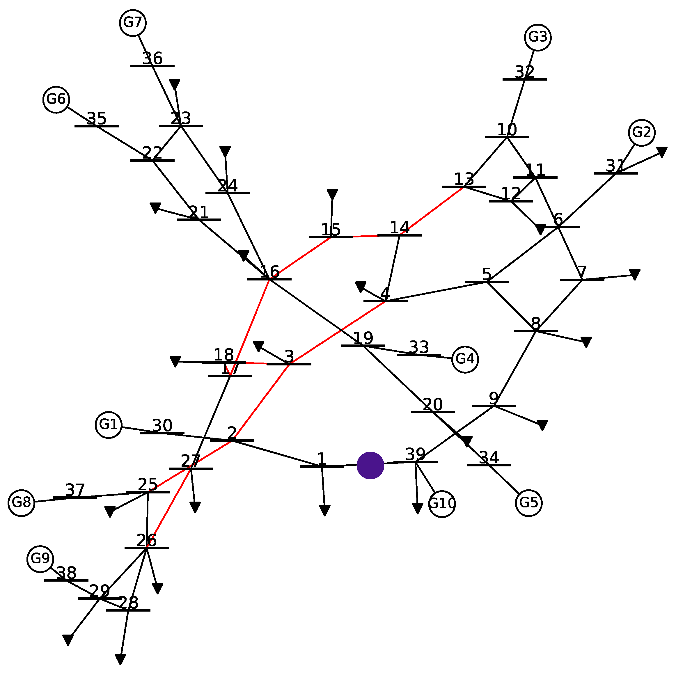
We now examine a larger example, namely the IEEE 39 test case, which contains 39 buses, 46 transmission lines, 10 generators, and 21 loads as shown in Figure 5. The properties of the transmission lines, generators, and loads are based on the MATPOWER test cases [25]. To generate diverse usage scenarios, we proceed as follows. We start with an hourly load profile curve aggregated for a single country. Here, we use the Danish load from 28 September 2020 and 27 September 2021 to generate 8735 scenarios [26]. To obtain nodal load time series that are both realistically correlated but are also partly independent of each other, we normalize the given load curve by its maximum value to yield , , and add randomness as follows:
where is the nominal value given in the IEEE test case for load i, and is a sample of the uniform distribution . Merit order is used for the dispatch of the generators where the dispatch cost of a generator is taken proportional to the inverse of its maximum active power output.
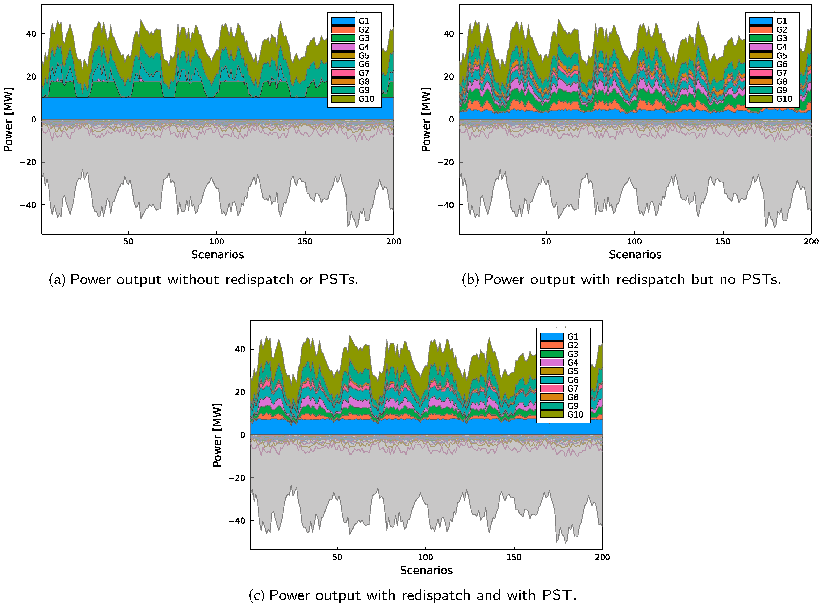
In Figure 6a, we show the dispatch of the generators for the first 200 consecutive time steps. The system without redispatch or PSTs is infeasible for the generated scenarios in the sense that the power flow over some transmission lines is larger than their capacity. We show in Figure 5 the transmission lines with the largest violations in red.
In Figure 6b, we show the power output of the generators when following the computed redispatch policy without any PST. This is achieved for very high PST installation costs in the MILP (14) problem. The optimal redispatch policy makes the power flow feasible for all scenarios, and the worst-case redispatch cost is ¤. The cheap generator G1 produces less power than is economically optimal without considering grid constraints.
For Figure 6c, we solve the MILP (14), now lowering the PST installation costs significantly. With these settings, the algorithm proposes to install 1 PST between buses 1 and 39 as shown in Figure 5. Given this decision, it is possible to reduce the worst-case redispatch cost to ¤ by using more power from the cheaper generator G1.
Optimality versus computation time is examined in Table 1, comparing the MILP and the greedy algorithm proposed in Section 6 for the same setting. The greedy algorithm is run with two different values of . With equal to , the algorithm does not propose the installation of any PST. If the value of is decreased to , the algorithm finds a better solution that yields ¤ for the worst-case redispatch cost, an increase of compared to the optimal solution of the MILP. In this solution, a PST is installed between buses 2 and 3.
Using a local compute node with 22 cores, MILP optimality with a 10% gap was proven after 5 h and 48 min. While acceptable for grid-planning purposes, the computation time is relatively high. In the configuration with equal to , the computation time of the greedy algorithm is 116 times faster than solving the MILP, and it is times faster for equal to . One could further improve the computational time of both the MILP and the proposed algorithm by, for example, restricting the affine linear maps to depend on principal components of the in-feeds only, thereby reducing the dimensions of and . Nevertheless, Table 1 shows that the proposed greedy algorithm outputs near-optimal objective values while being much faster to solve than the original MILP. The results show that the hill-climbing approach could be a valuable tool in preliminary analyses of PST placement, where sub-optimal solutions are acceptable. Then, once the final model is defined, the MILP can be run to find the optimal placement solution.
8. Conclusions
In this work, we presented an algorithm to find the minimal set of PSTs and the optimal phase shift and redispatch policies that enable the feasible operation of the transmission system for a continuous set of uncertain in-feed scenarios. We demonstrated our algorithm with two examples, proving that only considering a few extreme scenarios may not be sufficient to guarantee feasible grid states under all conditions and that the PST placement can significantly reduce the worst-case redispatch cost. The experiments also show that a proposed greedy algorithm can compute solutions much faster than the MILP, making it suitable for preliminary analyses on large grids. The proposed methodology can be easily extended to solve the optimal placement problem of different FACTS devices as long as a linear relationship model exists between their actuation and the grid power flow.
Author Contributions
Conceptualization, A.S. and F.S.; methodology, A.S.; software, A.S.; validation, A.S. and F.S.; formal analysis, A.S. and F.S.; investigation, A.S. and F.S.; resources, A.S.; data curation, A.S.; writing—original draft preparation, A.S. and F.S.; writing—review and editing, A.S. and F.S.; visualization, A.S.; supervision, F.S.; project administration, F.S.; funding acquisition, F.S. All authors have read and agreed to the published version of the manuscript.
Funding
This research was funded by the German Federal Ministry of Education and Research in project AlgoRes (grant no. 01|S18066A). It was performed in the context of the LOEWE center emergenCITY. We acknowledge support by the Deutsche Forschungsgemeinschaft (DFG, German Research Foundation) and the Open Access Publishing Fund of Technical University of Darmstadt.
Data Availability Statement
Not applicable.
Conflicts of Interest
The authors declare no conflict of interest. The funders had no role in the design of the study; in the collection, analyses, or interpretation of data; in the writing of the manuscript; or in the decision to publish the results.
References
- Proposed terms and definitions for flexible AC transmission system (FACTS). IEEE Trans. Power Deliv. 1997, 12, 1848–1853. [CrossRef]
- Gerbex, S.; Cherkaoui, R.; Germond, A.J. Optimal location of multi-type FACTS devices in a power system by means of genetic algorithms. IEEE Trans. Power Syst. 2001, 16, 537–544. [Google Scholar] [CrossRef]
- Duan, C.; Fang, W.; Jiang, L.; Niu, S. FACTS devices allocation via sparse optimization. IEEE Trans. Power Syst. 2015, 31, 1308–1319. [Google Scholar] [CrossRef]
- Lima, F.G.; Galiana, F.D.; Kockar, I.; Munoz, J. Phase shifter placement in large-scale systems via mixed integer linear programming. IEEE Trans. Power Syst. 2003, 18, 1029–1034. [Google Scholar] [CrossRef]
- Mínguez, R.; Milano, F.; Zárate-Miñano, R.; Conejo, A.J. Optimal network placement of SVC devices. IEEE Trans. Power Syst. 2007, 22, 1851–1860. [Google Scholar] [CrossRef]
- Xu, X.; Zhao, J.; Xu, Z.; Chai, S.; Li, J.; Yu, Y. Stochastic optimal TCSC placement in power system considering high wind power penetration. IET Gener. Transm. Distrib. 2018, 12, 3052–3060. [Google Scholar] [CrossRef]
- Zhang, X.; Shi, D.; Wang, Z.; Zeng, B.; Wang, X.; Tomsovic, K.; Jin, Y. Optimal allocation of series FACTS devices under high penetration of wind power within a market environment. IEEE Trans. Power Syst. 2018, 33, 6206–6217. [Google Scholar] [CrossRef]
- Frolov, V.; Thakurta, P.G.; Backhaus, S.; Bialek, J.; Chertkov, M. Operations- and uncertainty-aware installation of FACTS devices in a large transmission system. IEEE Trans. Control. Netw. Syst. 2019, 6, 961–970. [Google Scholar] [CrossRef]
- Roald, L.; Misra, S.; Krause, T.; Andersson, G. Corrective control to handle forecast uncertainty: A chance constrained optimal power flow. IEEE Trans. Power Syst. 2016, 32, 1626–1637. [Google Scholar] [CrossRef]
- Bienstock, D.; Chertkov, M.; Harnett, S. Chance-constrained optimal power flow: Risk-aware network control under uncertainty. Siam Rev. 2014, 56, 461–495. [Google Scholar] [CrossRef]
- Vrakopoulou, M.; Margellos, K.; Lygeros, J.; Andersson, G. A Probabilistic Framework for Reserve Scheduling and N-1 Security Assessment of Systems With High Wind Power Penetration. IEEE Trans. Power Syst. 2013, 28, 3885–3896. [Google Scholar] [CrossRef]
- Momoh, J.; Ma, X.; Tomsovic, K. Overview and literature survey of fuzzy set theory in power systems. IEEE Trans. Power Syst. 1995, 10, 1676–1690. [Google Scholar] [CrossRef]
- Thukaram, D.; Jenkins, L.; Visakha, K. Improvement of system security with unified-power-flow controller at suitable locations under network contingencies of interconnected systems. IEE Proc.-Gener. Transm. Distrib. 2005, 152, 682–690. [Google Scholar] [CrossRef]
- Yan, S.; Gu, Z.; Park, J.H.; Xie, X. Sampled Memory-Event-Triggered Fuzzy Load Frequency Control for Wind Power Systems Subject to Outliers and Transmission Delays. IEEE Trans. Cybern. 2022, 53, 4043–4053. [Google Scholar] [CrossRef]
- Suganthi, L.; Iniyan, S.; Samuel, A.A. Applications of fuzzy logic in renewable energy systems—A review. Renew. Sustain. Energy Rev. 2015, 48, 585–607. [Google Scholar] [CrossRef]
- Wold, S.; Esbensen, K.; Geladi, P. Principal component analysis. Chemom. Intell. Lab. Syst. 1987, 2, 37–52. [Google Scholar] [CrossRef]
- Geng, S.; Vrakopoulou, M.; Hiskens, I.A. Chance-constrained optimal capacity design for a renewable-only islanded microgrid. Electr. Power Syst. Res. 2020, 189, 106564. [Google Scholar] [CrossRef]
- Dubey, R.; Dixit, S.; Agnihotri, G. Optimal placement of shunt FACTS devices using heuristic optimization techniques: An Overview. In Proceedings of the 2014 Fourth International Conference on Communication Systems and Network Technologies, Bhopal, India, 7–9 April 2014; IEEE: Piscataway, NJ, USA, 2014; pp. 518–523. [Google Scholar]
- Jordehi, A.R.; Jasni, J. Heuristic methods for solution of FACTS optimization problem in power systems. In Proceedings of the 2011 IEEE Student Conference on Research and Development, Cyberjaya, Malaysia, 19–20 December 2011; IEEE: Piscataway, NJ, USA, 2011; pp. 30–35. [Google Scholar]
- Ahmad, A.A.; Sirjani, R. Optimal placement and sizing of multi-type FACTS devices in power systems using metaheuristic optimisation techniques: An updated review. Ain Shams Eng. J. 2020, 11, 611–628. [Google Scholar] [CrossRef]
- Kundur, P.S.; Malik, O.P. Power System Stability and Control, 2nd ed.; McGraw Hill: New York, NY, USA, 2022. [Google Scholar]
- Dunning, I.; Huchette, J.; Lubin, M. JuMP: A Modeling Language for Mathematical Optimization. SIAM Rev. 2017, 59, 295–320. [Google Scholar] [CrossRef]
- Gurobi Optimization, LLC. Gurobi Optimizer Reference Manual. 2023. Available online: https://www.gurobi.com (accessed on 6 September 2021).
- Ptacek, J.; Modlitba, P.; Vnoucek, S.; Cermak, J. Possibilities of applying phase shifting transformers in the electric power system of the Czech Republic. In Proceedings of the CIGRE Session 2006, Paris, France, 22–25 August 2006; pp. 2–203. [Google Scholar]
- Zimmerman, R.D.; Murillo-Sánchez, C.E.; Thomas, R.J. MATPOWER: Steady-state operations, planning, and analysis tools for power systems research and education. IEEE Trans. Power Syst. 2010, 26, 12–19. [Google Scholar] [CrossRef]
- Energinet.dk. Production and Consumption Data. Available online: https://energinet.dk (accessed on 6 September 2021).
Figure 1.
We propose an efficient planning algorithm to improve the power flow controllability of transmission grids, taking into account the various operational options of the TSO (green). The approach is robust against key influencing factors (red).
Figure 1.
We propose an efficient planning algorithm to improve the power flow controllability of transmission grids, taking into account the various operational options of the TSO (green). The approach is robust against key influencing factors (red).

Figure 2.
Uncertainty set defined as the intersection of the smallest non-rotated hyperrectangle that encloses all scenarios, and a rotated hyperrectangle in the direction of the data’s principal components that also encloses all scenarios. (Plot inspired by [17]).
Figure 2.
Uncertainty set defined as the intersection of the smallest non-rotated hyperrectangle that encloses all scenarios, and a rotated hyperrectangle in the direction of the data’s principal components that also encloses all scenarios. (Plot inspired by [17]).

Figure 3.
3-bus test grid. A gas power plant (red) and a load are connected to bus 1, while a lignite power plant (brown) and a wind park (blue) are connected to bus 2. A second, smaller wind park (light blue) is connected to bus 3. A PST is added to line (1,3) for a small enough installation cost .

Figure 4.
Varying the total wind power in-feed for the 3-bus test grid in Figure 3. (a) Scenario-wise optimized redispatch (solid) and affine-linear redispatch policy (dashed) without a PST and (b) with PST. (c) The corresponding redispatch costs. (d) Optimal affine PST policy in case a PST is installed (black) and redirected power flow (gray).

Figure 5.
Topology of IEEE 39 bus test case. The lines marked in red have the largest capacity violations when solving the power flow without redispatch or PSTs. The shaded circle denotes the location proposed by our algorithm for installing a PST.
Figure 5.
Topology of IEEE 39 bus test case. The lines marked in red have the largest capacity violations when solving the power flow without redispatch or PSTs. The shaded circle denotes the location proposed by our algorithm for installing a PST.

Figure 6.
Power output of the 10 generators of the IEEE 39 system for 200 consecutive time steps. The gray area represents the total power demand. (a) The power output is defined by merit order, where the production cost is inversely proportional to the generator maximum active power output. (b) The power output is defined by the dispatch plus the redispatch generated by the optimal redispatch policy found using the proposed algorithm. (c) Same as (b) but with a PST installed between buses 1 and 39.


Table 1.
Performance evaluation of MILP and greedy algorithm .
| Cost [¤] | Time [] | PSTs | |
|---|---|---|---|
| MILP | 1.93 | 348 | 1 |
| () | 3.30 | 3 | 0 |
| () | 2.25 | 8 | 1 |
Disclaimer/Publisher’s Note: The statements, opinions and data contained in all publications are solely those of the individual author(s) and contributor(s) and not of MDPI and/or the editor(s). MDPI and/or the editor(s) disclaim responsibility for any injury to people or property resulting from any ideas, methods, instructions or products referred to in the content. |
© 2023 by the authors. Licensee MDPI, Basel, Switzerland. This article is an open access article distributed under the terms and conditions of the Creative Commons Attribution (CC BY) license (https://creativecommons.org/licenses/by/4.0/).
Share and Cite
MDPI and ACS Style
Santos, A.; Steinke, F. Robust Placement and Control of Phase-Shifting Transformers Considering Redispatch Measures. Energies 2023, 16, 4438. https://doi.org/10.3390/en16114438
AMA Style
Santos A, Steinke F. Robust Placement and Control of Phase-Shifting Transformers Considering Redispatch Measures. Energies. 2023; 16(11):4438. https://doi.org/10.3390/en16114438
Chicago/Turabian StyleSantos, Allan, and Florian Steinke. 2023. "Robust Placement and Control of Phase-Shifting Transformers Considering Redispatch Measures" Energies 16, no. 11: 4438. https://doi.org/10.3390/en16114438
Note that from the first issue of 2016, this journal uses article numbers instead of page numbers. See further details here.