
On Training Data Selection in Condition Monitoring Applications—Case Azimuth Thrusters


1
Control Engineering, Environmental and Chemical Engineering, University of Oulu, P.O. Box 4300, 90014 Oulu, Finland
2
Kongsberg Maritime AS, P.O. Box 1522, N-6065 Ulsteinvik, Norway
*
Author to whom correspondence should be addressed.
Appl. Sci. 2022, 12(8), 4024; https://doi.org/10.3390/app12084024
Submission received: 20 December 2021
/
Revised: 13 April 2022
/
Accepted: 14 April 2022
/
Published: 15 April 2022
(This article belongs to the Special Issue Health Monitoring of Mechanical Systems)
Abstract
:Machine learning techniques are commonly used in the vibration-based condition monitoring of rotating machines. However, few research studies have focused on model training from a practical viewpoint, namely, how to select representative training samples and operating areas for monitoring applications. We focus on these aspects by studying training sets with varying sizes and distributions, including their effects on the models to be identified. The analysis is based on acceleration and shaft speed data available from an azimuth thruster of a catamaran crane vessel. The considered machine learning algorithm was previously introduced in another study suggesting it could detect defects on the thruster driveline components. In this work, practical guidance is provided to facilitate its implementation, and furthermore, an adaptive method for training subset selection is proposed. Results show that the proposed method enabled the identification of usable training subsets in general, while the success of the previous approach was case-dependent. In addition, the use of Kolmogorov–Smirnov or Anderson–Darling tests for normal distribution, as a part of the method, enabled selections that covered the operating area broadly, while other tests were unfavorable in this regard. Overall, the study demonstrates that reconfigurable and automated model implementations could be achievable with minor effort.
1. Introduction
Nowadays, companies collect large amounts of data as the result of the recent progress in industrial digitalization [1]. Regardless, systematic data exploitation can still be seen as incomplete [2] while the approaches to data management and processing are unestablished. In industrial maintenance and condition monitoring (CM), machine learning (ML) methods have become an intriguing option for data analysis because they could recognize the health states of machines automatically [3]. However, the research on this field is widely realized with simulation data and data from precisely controlled laboratory tests, which are commonly free from the characteristics of industrial data, such as noise, inconsistency, outliers, incomplete records, irrelevant samples, unfavorable and varying operating areas and the lack of labeled samples [4,5,6]. In addition, the data for model training are commonly selected manually and the introduction of their characteristics may not be explicit [7]. The usability of trained models remains largely uncertain when their connections with data characteristics are poorly understood. On the other hand, the automated methods for sample selection [8,9,10] could pave the way towards reproducible solutions that are needed in the practical applications of ML. There, a single application is potentially transferred into various instances requiring robustness, automated properties and easy reconfigurability.
The most common approach to machine learning is supervised learning [11] where the model training is based on known (or labeled) samples. The sample selection for training data is usually conducted as a pre-processing step [4,5] and it often requires many trials to achieve a usable model. In common practice, the sample selection equals the elimination of samples that are noisy, redundant, or irrelevant in available datasets, and it is often realized through a manual procedure. Additionally, automated feature selection and dimensionality reduction techniques are applied to reduce the data dimensions, namely, the number of predictor variables to ease the learning process [12]. The importance of automated data selection is increasingly noted because firstly, the volume of data is expected to grow in modern computational applications [1,13] and secondly, large datasets tend to increase information redundancy and complexity, leading to low prediction precision and to decreased computational efficiency in data-driven modeling [9,14].
The recent literature on monitoring of rotating machines based on ML methods is commonly focused on the prediction performance of classifiers [3,15], but the reasoning for training data selection remains unclear. However, it is often mentioned that the training samples should enable the most accurate generalization [16]. In addition, they should be sampled from a broad distribution across the input space to contain the natural variability of the quantities in use [9]. On the other hand, all the data from such a distribution are not equally useful in model training [17] and random selection is then impractical. In industrial applications, training data are typically hand-picked based on the status codes given by the monitoring system [4,12] and based on expert knowledge [6]. The fault data of rotating machines, collected into data repositories, typically have drawbacks such as the narrow coverage of the complete operating area or poor quality. Moreover, each unique fault may show new, previously unseen symptoms in indirect measurements, such as acceleration signals. Therefore, the data of fault-free operating conditions solely are commonly applied for model training [4,5,6,12,18]. The one-class classifier is then used for anomaly detection.
However, the problem of training data selection is mainly approached from the perspective of maximizing the generalization performance in classification [19] by finding the smallest set of samples [8] with the assumption that representative data are available in more than one class. The selection strategies include the pruning of redundant samples [9], evolutionary computation methods [10], methods combining feature selection and data sampling [16] and experimental design techniques [20,21]. In addition, various studies focus on sample selection for specific algorithms, such as support vector machines [9,22,23], decision tree classifiers [16], nearest neighbor classifiers [19] and neural networks [20]. Such methods are beneficial for specific training sets containing representative data of classes. By contrast, this study focuses on selecting the training subsets that define representative operating areas for condition monitoring based on one class instead of trying to maximize the classification performance. The operating areas are defined by a single variable, namely, the shaft rotational speed, because it is commonly available in rotating machines including azimuth thrusters. This approach enables the rejection of unfavorable operating areas for monitoring, and furthermore, the selection process is unaffected by the case-specific fault conditions, which improves its general applicability.
Furthermore, industrial systems typically change during operation, which causes a dataset shift [24]. The detection of shifted datasets [25,26] and adaptation to them [27,28] are general goals in ML development that aim at practical implementation. Therefore, the data selection procedure is analyzed in this study with multiple datasets collected in chronological order during operation.
The study was made by applying the probabilistic condition monitoring algorithm introduced in [6] on the datasets collected from a single azimuth thruster. While the previous work [6] was focused on describing the algorithm for anomaly detection, this work clarifies the effect of training data on the system identification procedure of the algorithm. The performance is studied based on relatively large datasets which were not available in the previous work. More specifically, the main contributions of the study can be summarized as follows. The effects of training data on the automatically selected training subsets are illustrated, and the model adaptation to different datasets is analyzed. The ‘training subset selection’ process of the algorithm is analyzed by using the original approach for dataset segmentation, and a new, more flexible approach suitable for large datasets with varying distributions is presented. The automated selection of training subsets is based on identifying the shaft speed ranges that exhibit normal distribution in the regression residuals of predicted features. Therefore, various hypothesis tests, such as Kolmogorov—Smirnov (KS) [29], Anderson–Darling (AD) [30], Lilliefors’ test [31], Jarque–Bera (JB) [32] and Shapiro–Wilk (SW) [33], are also compared as a part of the selection process. The case study provides guidance for the implementation of the considered condition monitoring algorithm. In addition, the approach to training data selection with the purpose of identifying the operating areas in place of maximizing the classification performance gives a practical viewpoint to the use of automated supervised learning in industrial condition monitoring.
2. Materials and Methods
This section presents the process for training subset selection from available data. The competing approaches to dataset segmentation and normal distribution testing are discussed. In addition, the data for algorithm training in the case of azimuth thruster condition monitoring are described.
2.1. Training Subset Selection
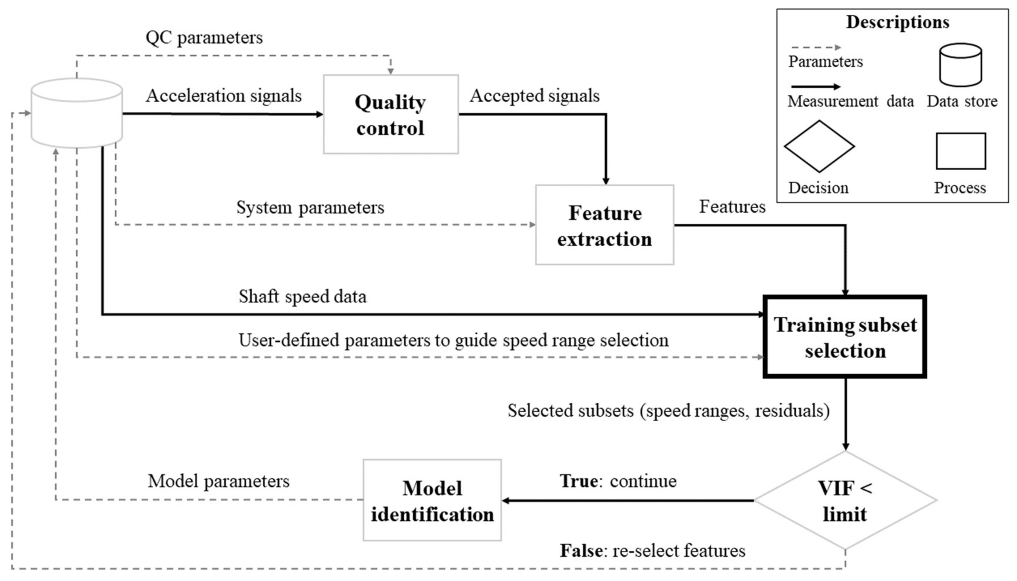
The algorithm for identifying CM models was originally presented in [6] and a flowchart of its stages is shown in Figure 1. The training subset selection process is highlighted there. It controls simultaneously the sample selection within the full training set and the selection of operating areas for monitoring. The process uses features extracted from the acceleration signal, the values of shaft rotational speed and user-defined parameters to guide the selection. The process checks the available samples in various operating areas, defined by the ranges of rotational speed values within the training subsets, and finally selects the subsets suitable for model training. To clarify, the process was named ‘speed range selection’ in the original version [6], but the name is modified here to refer to the more general concept of training data selection.
The main function of training data selection is to identify the subsets in which the predictions of linear regression models result in residuals that are normally distributed. The regression models utilize shaft speed values to predict the values of vibration features. Therefore, a residual (ri) can be defined as
where yi is a calculated feature value, xi is a shaft speed value and i is the sample number. Parameters β0 and β1 are the intercept and the regression coefficient, respectively.
ri = yi − β0 − β1xi,
The selected features are described in Table 1 and their residuals were monitored together in suitable combinations. Features 1–3 were selected for the time-domain model, features 4–8 for the bearing model and features 9–11 for the gear model. The reasoning for the selected features, the system parameters for their calculation and the use of their residuals for condition monitoring were presented in [6]. The applied system parameters included Ball Pass Frequency Inner Race (BPFI), Ball Pass Frequency Outer Race (BPFO), Ball Spin Frequency (BSF), Fundamental Train Frequency (FTF) and Gear Mesh Frequency (GMF).
As shown in Figure 1, the algorithm uses preset parameters that control its performance, and it gives model parameters that are identified during training. The preset parameters that guide the speed range selection are defined in Section 2.1.1. The studied model parameters given by the algorithm include the rotational speed ranges and the confidence intervals of regression coefficients.
The applied quality control (QC) parameters are the same as in the previous study [6], namely, the moving window size is 100 acceleration values, the limit for the range of moving mean range is 0.5 g and the limit for the absolute mean of the signal is 2 g. However, the absolute mean check was unnecessary in the case study where the signal offset was removed by the system onboard. The algorithm uses variance inflation factor (VIF) values to assess the multicollinearity of residual sets. For the sake of brevity, the analysis of such values is omitted here, but to clarify, they were strictly <10 based on random sampling.
2.1.1. Dataset Segmentation
The training subset selection process identifies the widest acceptable operating ranges, based on shaft rotational speed, without any overlap between each other. To have an acceptable range, the residual sets must be normally distributed in the data, as shown in [6]. A single residual set refers to the differences between the values of a feature and its predicted values by linear regression fitted on the training subset, see Equation (1).
In our previous work [6], the distribution of shaft speed values was divided into 55 ranges based on the deciles so that all the values between the minimum and maximum of the dataset were used. In this work, this approach is termed ’basic training subsets’. The minimum number of samples that are accepted within a range (or subset) was set to 10% of the sample size (N) of the dataset in the tests presented here.
Additionally, a new approach was proposed, where the distribution of shaft speed values was segmented into 4851 separate ranges, based on percentiles. The values from the 1st to 99th percentile were processed so that the candidate ranges were one percentage point wide at minimum and 98 percentage points at maximum (namely, the interval between the 1st and 99th percentiles). The first range covered values between 1st and 2nd percentiles, the second covered values between 1st and 3rd percentiles, the third covered values between 1st and 4th percentiles and so forth. The lower end of ranges consisted of 1–98th percentiles and the upper end consisted of 2–99th percentiles.
However, the proposed approach may result in impractically narrow ranges, and therefore, the minimum width (in rpm) was introduced as another user-defined parameter to guide the speed range selection. The minimum width was set to 5 rpm and the narrower ranges were then removed from the full set of ranges (4851 ranges). Furthermore, the ranges were required to include at least 40 samples to be accepted. Consequently, the number of subsets considered was different for each complete training set. This approach is termed ‘adaptive training subsets’ to describe its dense segmentation of distribution and high flexibility compared with the previous approach. The main differences between the approaches to dataset segmentation are summarized in Table 2.
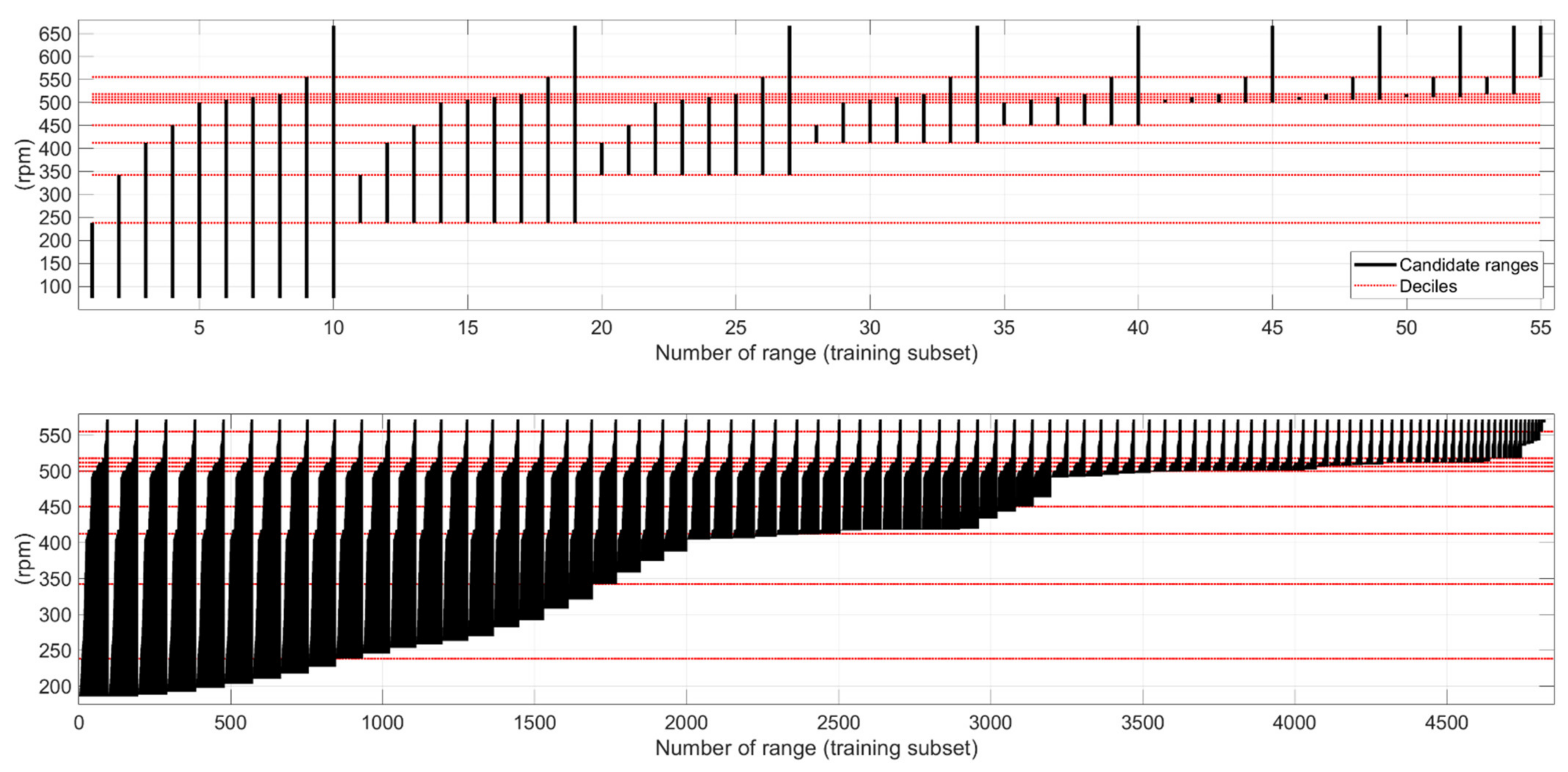
Figure 2 illustrates the candidates for shaft speed ranges with one training set (N = 3000) that is later introduced in Section 2.2. ‘Basic training subsets’ approach is shown on top in Figure 2, whereas ‘adaptive training subsets’ is shown below. The plot on top shows that in the case of a skewed distribution with many samples, the adjacent candidate ranges may have large differences in the boundary values with ‘basic training subsets’ approach. For example, the lower value of the candidate ranges jumps from 239 rpm to 343 rpm when the lower end shifts from the 20th to 30th percentile (see ranges 11–27). The plot below illustrates that ‘adaptive training subsets’ approach with thousands of candidate subsets introduces more flexibility to the range selection due to the higher resolution.
2.1.2. Applied Hypothesis Tests
Five well-known hypothesis tests were applied for testing the normal distribution of the residual sets. Most of these tests belong to the group of empirical distribution function tests, where the difference between the empirical and hypothesized cumulative distributions is evaluated. From that group, Kolmogorov–Smirnov [29], Anderson–Darling [30] and Lilliefors’ tests [31] were selected. KS and Lilliefors’ tests belong to the supremum class of methods where the greatest vertical difference between the hypothesized and empirical distribution is evaluated. In KS test, the hypothesized distribution is completely specified, whereas in Lilliefors’ test, the parameters are estimated based on the sample. Furthermore, AD test comes from the class of quadratic methods, where the squared difference between the empirical and hypothesized distributions is evaluated.
As categorized in [34], one test from the class of moment tests and one from the class of correlation tests were selected as well. Jarque–Bera belongs to the class of moment tests, where the deviation from normality is detected based on the third and fourth moments of the distribution, namely, skewness and kurtosis [32]. Finally, Shapiro–Wilk test is a correlation test based on the ratio of two estimates for scale obtained from order statistics [33].
The applied MATLAB® functions for KS, AD, Lilliefors’ and JB tests were kstest, adtest, lillietest and jbtest, respectively. SW was tested with the MATLAB® code provided by [35]. The standard 5% significance level was applied in all the hypothesis tests. The KS tests were conducted on the standardized residuals (μ = 0, σ = 1) and in the other tests the residuals were not standardized. In the AD test, the hypothesized normal distribution was generated based on the mean and standard deviation of the residual set by using the makedist function.
2.2. Description of Data
The following subsection introduces the source of data, namely, the thruster and the measurements. Then, the shaft speed data are described by focusing on the distribution of the tested datasets. The features extracted from acceleration samples are illustrated thereafter and their relation to the shaft speed shown.
2.2.1. Thruster and Measurements
The data for this study come from a UUC 455 thruster manufactured by Kongsberg Maritime Finland Oy. The data were collected during a campaign during April–May 2021 on ‘Pioneering Spirit’, the largest construction vessel in the world. Figure 3 presents a drawing of the thruster model with the main components of interest highlighted. The data from the piezoelectric accelerometer located next to the pinion shaft support bearing and gear were selected for analysis. The sampling rate varied based on the shaft speed. During one shaft revolution, 512 acceleration values were measured and the length of the complete time series in a sample was 16,384 values. Samples were collected roughly at 5-min intervals.
2.2.2. Shaft Speed Values
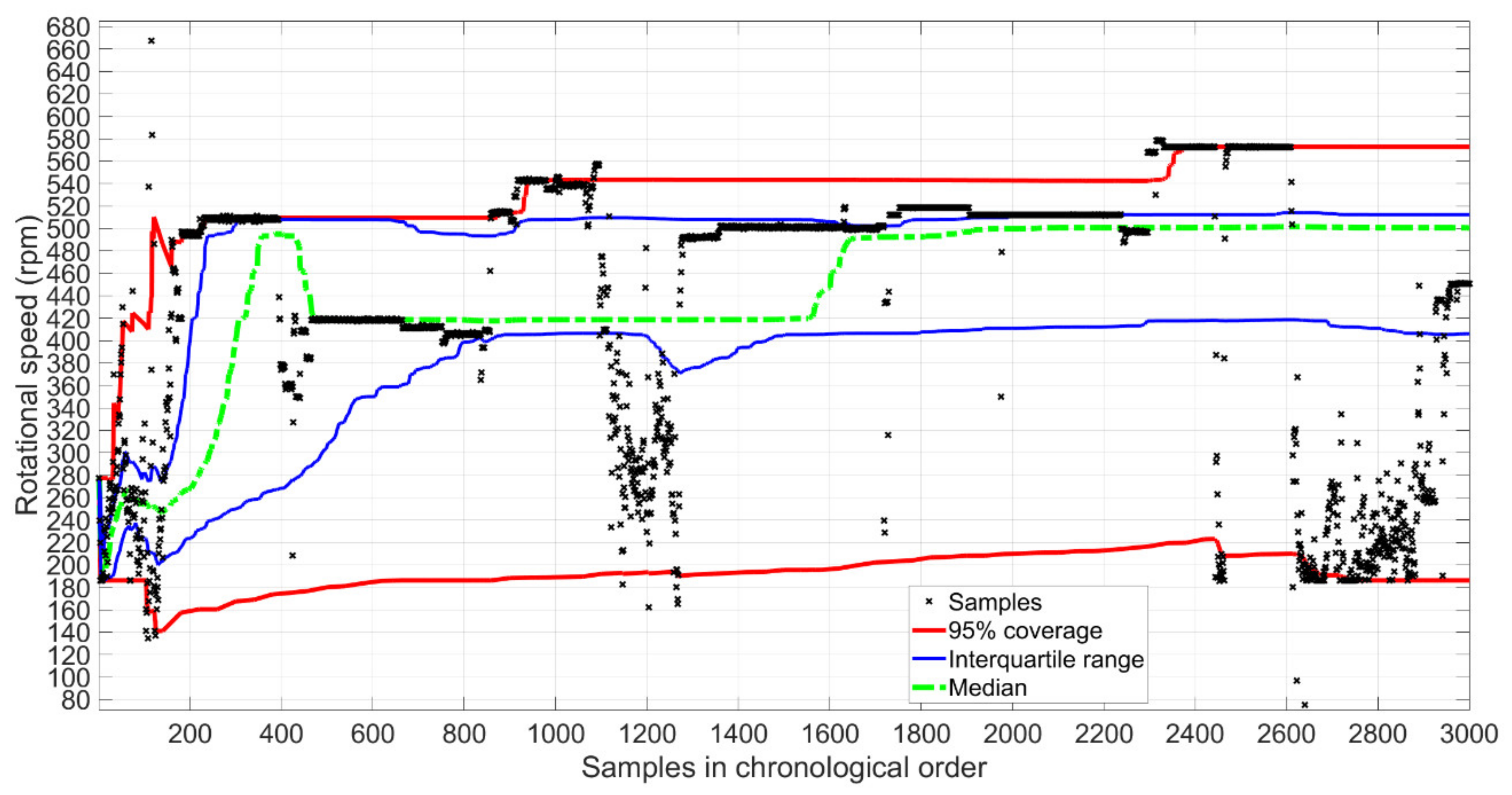
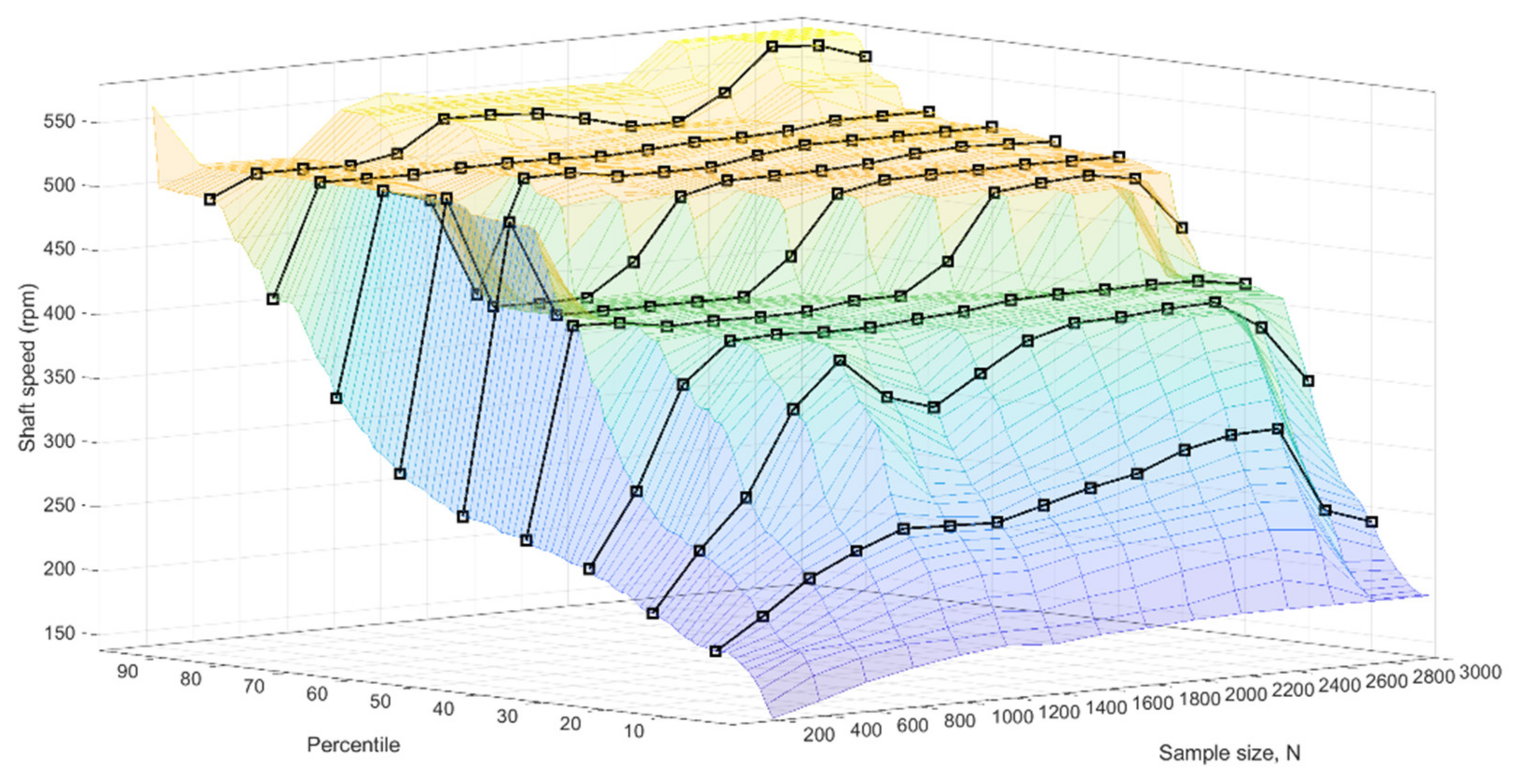
Figure 4 presents the shaft speed values during the monitored period in chronological order. In addition, the median, interquartile range and the 95% coverage are shown cumulatively so that each value is calculated based on all the values from the first one to the value of that time. To analyze the effect of sample size and distribution on the performance in training subset selection, the full dataset was chopped into different training sets with sizes from N = 200 to N = 3000 with the steps of 200 samples. Figure 5 illustrates the 1–99th percentiles of the different datasets generated.
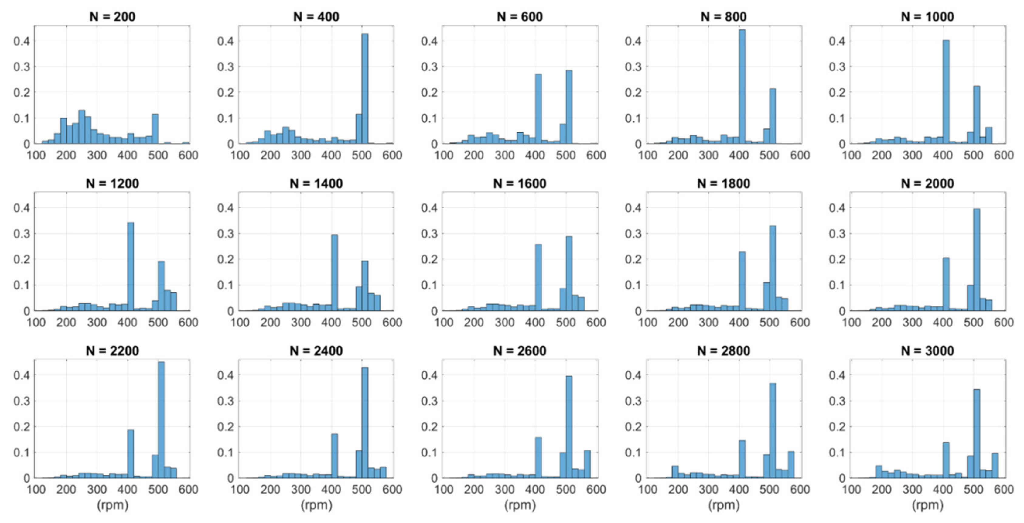
Figure 5 shows that the first 200 samples resulted in the most uniform distribution with some outlying values in the higher end (see also Figure 4). Thereafter, the thruster was commonly operated at shaft speeds around 500 rpm, with some periods of higher and lower speed. As shown in Figure 5, the median of datasets with sample sizes N = 600–1400 was around 419 rpm and increased to 500 rpm with the sample sizes N = 2000–3000. The interquartile range in Figure 4 shows that half of the samples were on a relatively narrow range (roughly 400–520 rpm) after the 800 first samples. The flat areas in Figure 5 indicate that large proportions of the samples in the distributions were collected from narrow operating areas. More details are shown in Appendix A.
2.2.3. Generated Feature Values
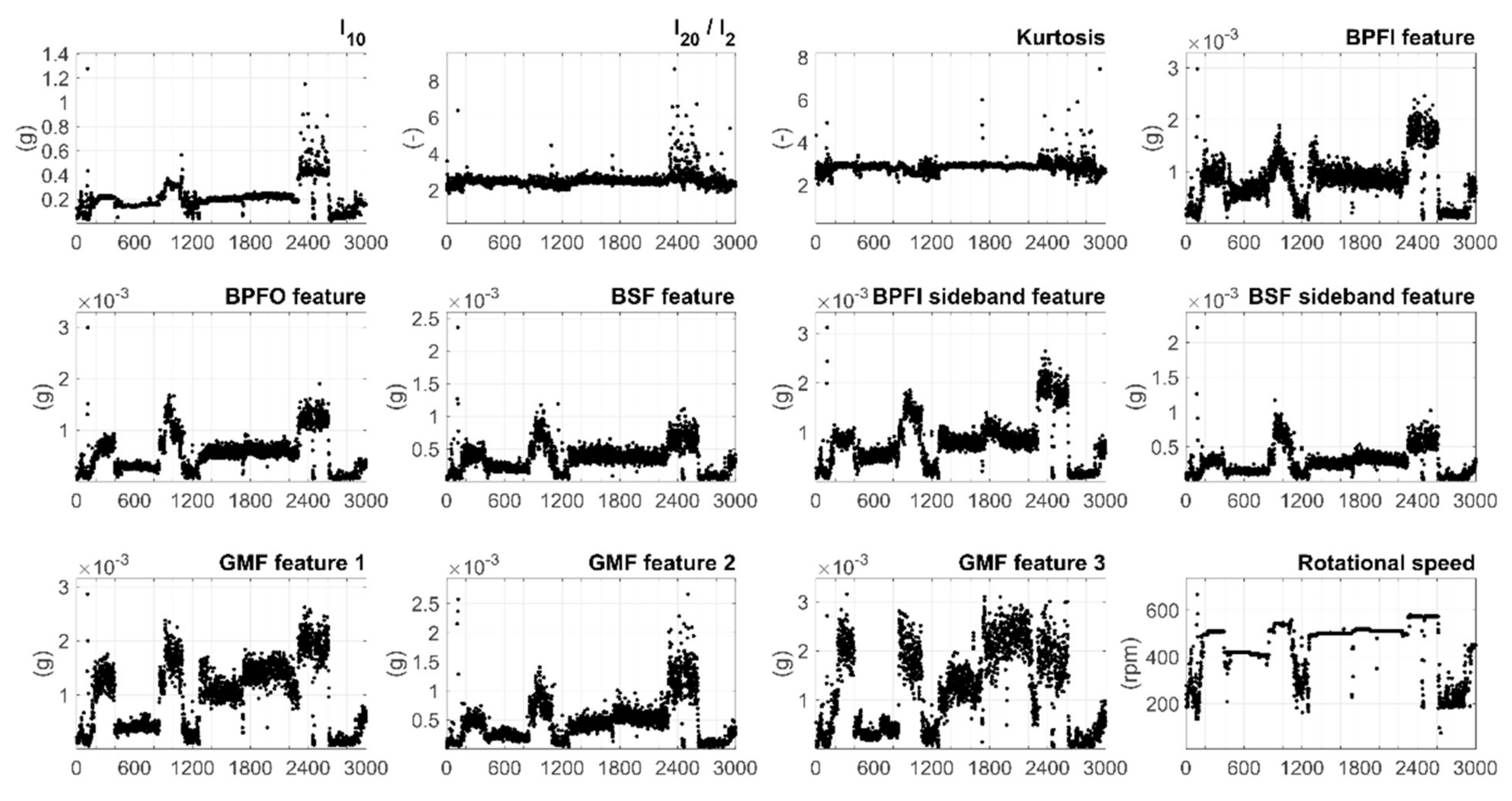
Figure 6 shows the feature values and shaft speed values in chronological order. The feature values followed the changes in the rotational speed values in a regular manner during the period which suggests that the monitored operation was relatively unchanged. Most feature values typically increased when the rotational speed increased considerably, but l20/l2 and kurtosis had a weak correlation with the shaft speed.
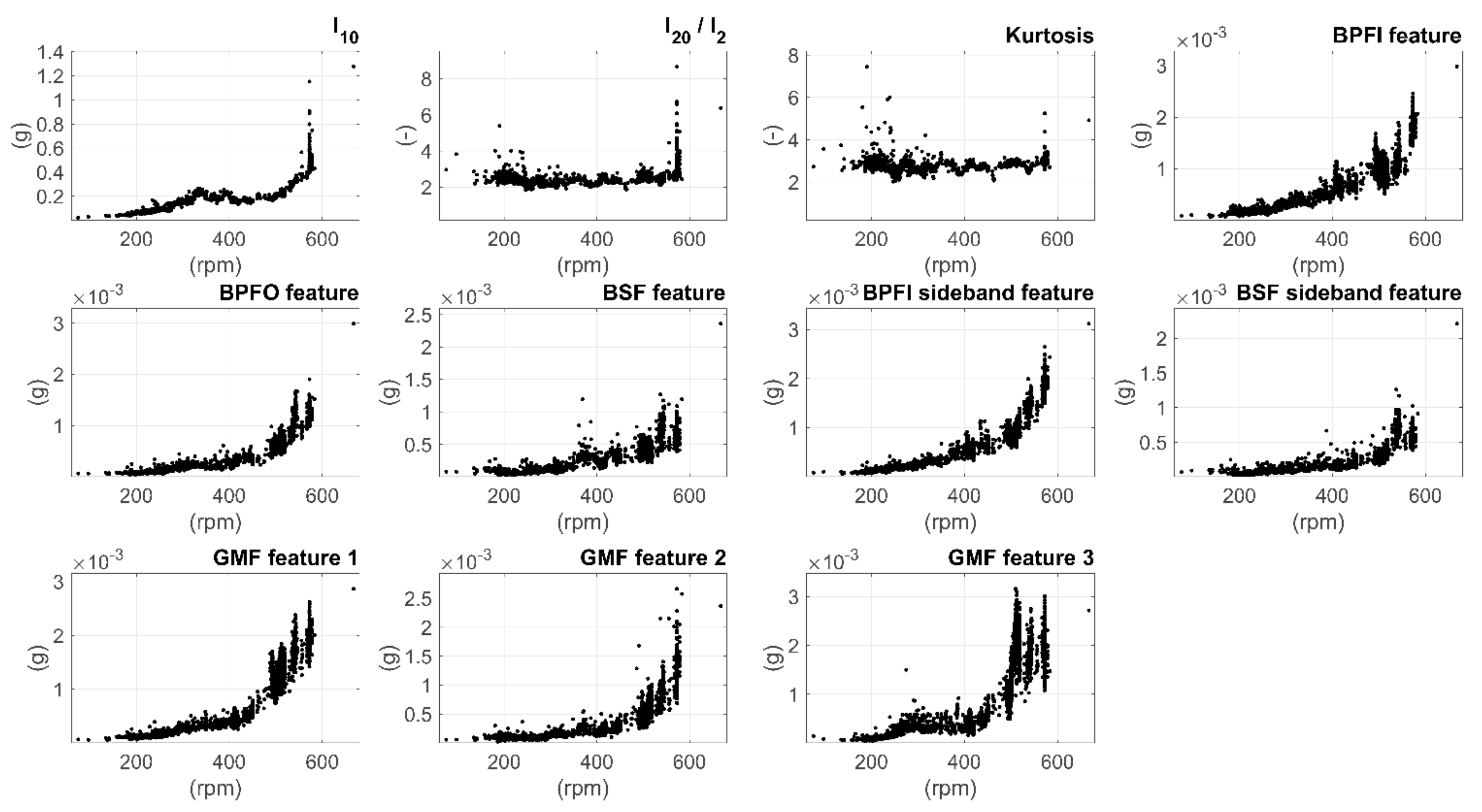
Figure 7 illustrates the correlation between the features and the shaft speed with scatter plots. Certain speed areas clearly resulted in high variation in the feature values. The high variation in kurtosis and l20/l2 roughly at 200-rpm speed could be explained by the steering angle changes during maneuvering, whereas the variation in many other features at the speed over 400 rpm is possibly a result of the ship movement during cruise. However, the effects of maneuvering and ship movements are left for future work.
3. Results
The following analysis focuses on the model training results from various viewpoints. In the first subsection, the proportion of acceptable training subsets is analyzed relative to the size of dataset. The number of selected subsets and the sizes of speed ranges for monitoring are illustrated thereafter. The third subsection shows the modeling error and parameter uncertainties for the linear regression of a single feature. Another aspect of significance, especially in the applications with limited computing capacity, is the computation time required for the system identification, and therefore, the time used in tests is analyzed in the fourth subsection. Finally, the results of different hypothesis tests for identifying normally distributed residuals are illustrated in the last subsection. The applied hypothesis test for normal distribution in Section 3.1, Section 3.2, Section 3.3 and Section 3.4 was Kolmogorov–Smirnov test.
3.1. Proportion of Acceptable Training Subsets
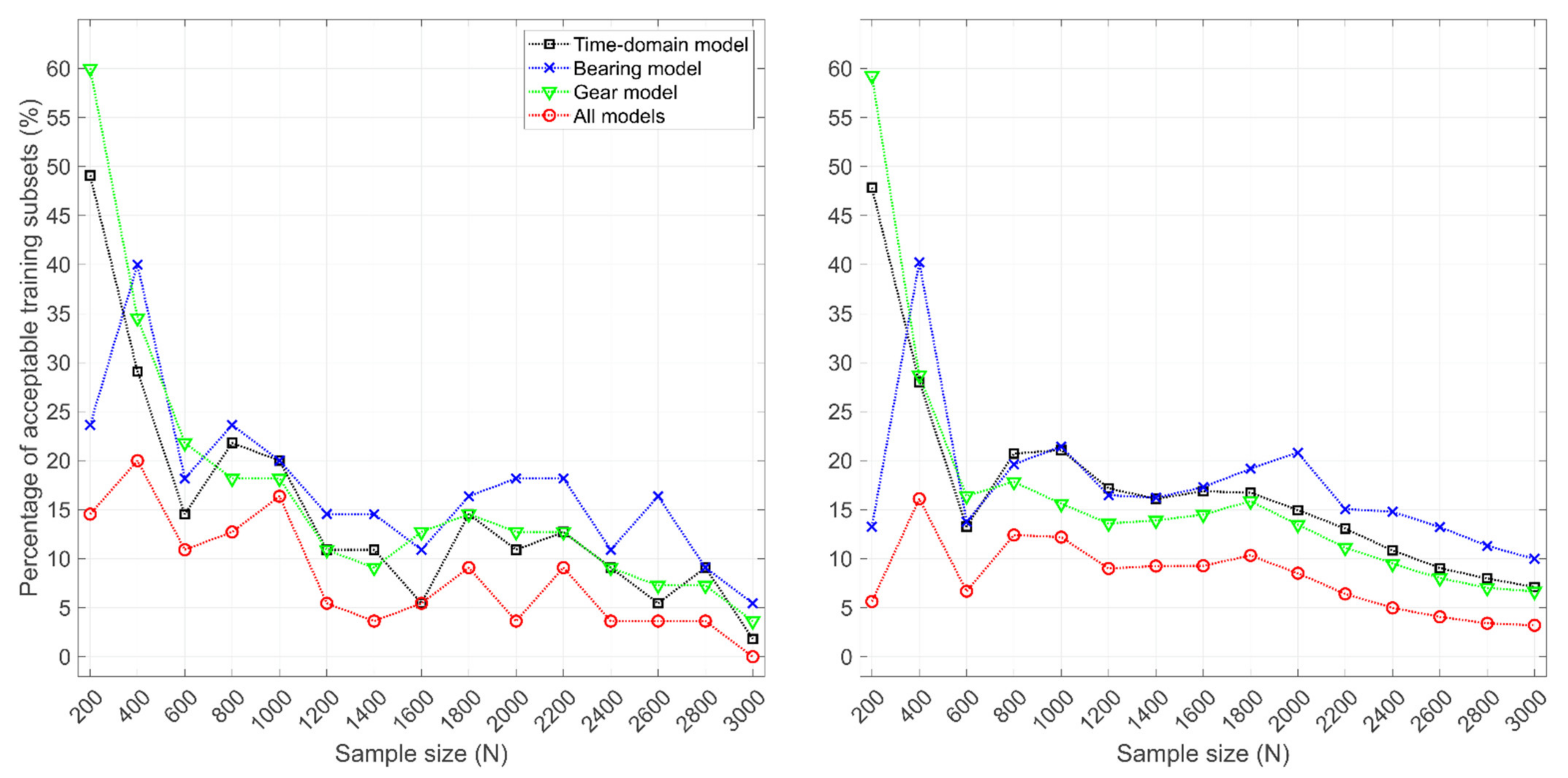
Figure 8 shows the percentage value of acceptable training subsets relative to the sample size of different datasets considered. The acceptable training subset means that the residual sets of all the considered features within the considered speed range were normally distributed within the subset. The quantity of the final selected training subsets was, however, lower than shown in Figure 8 when only the widest rotational speed ranges without overlap became selected for monitoring, as shown in Section 3.2.
Tests were conducted by using all eleven features together (all models) and separately in groups by using the time-domain model (features 1–3), the bearing model (features 4–8) and the gear model (features 9–11). With ‘basic training subsets’, the total number of subset candidates was 55 (see Figure 2), while the number varied with the ‘adaptive training subsets’ approach based on the dataset. The number of candidate subsets was then {3160, 3495, 3890, 4036, 4198, 4310, 4432, 4407, 4355, 4378, 4277, 4298, 4326, 4396, 4459} for the datasets with sizes from 200 to 3000 samples with the steps of 200 samples, respectively.
In general, the increasing size of the dataset resulted in the decreased percentage value of acceptable subsets. A large feature set, such as the case with ‘all models’, resulted in a lower number of acceptable subsets than the smaller feature sets. Both approaches to dataset segmentation resulted in a relatively similar proportion of acceptable subsets. However, the absolute number of acceptable subsets was much higher in the ‘adaptive training subsets’ approach. Moreover, the case of ‘all models’ and N = 3000 on the left had 0% acceptable subsets, whereas on the right, the corresponding result was 3.2%, which implies that the approach with thousands of training subset candidates is more useful with large datasets. Please refer to Appendix B for a similar analysis focusing on each feature separately.
3.2. Identified Operating Areas for Monitoring
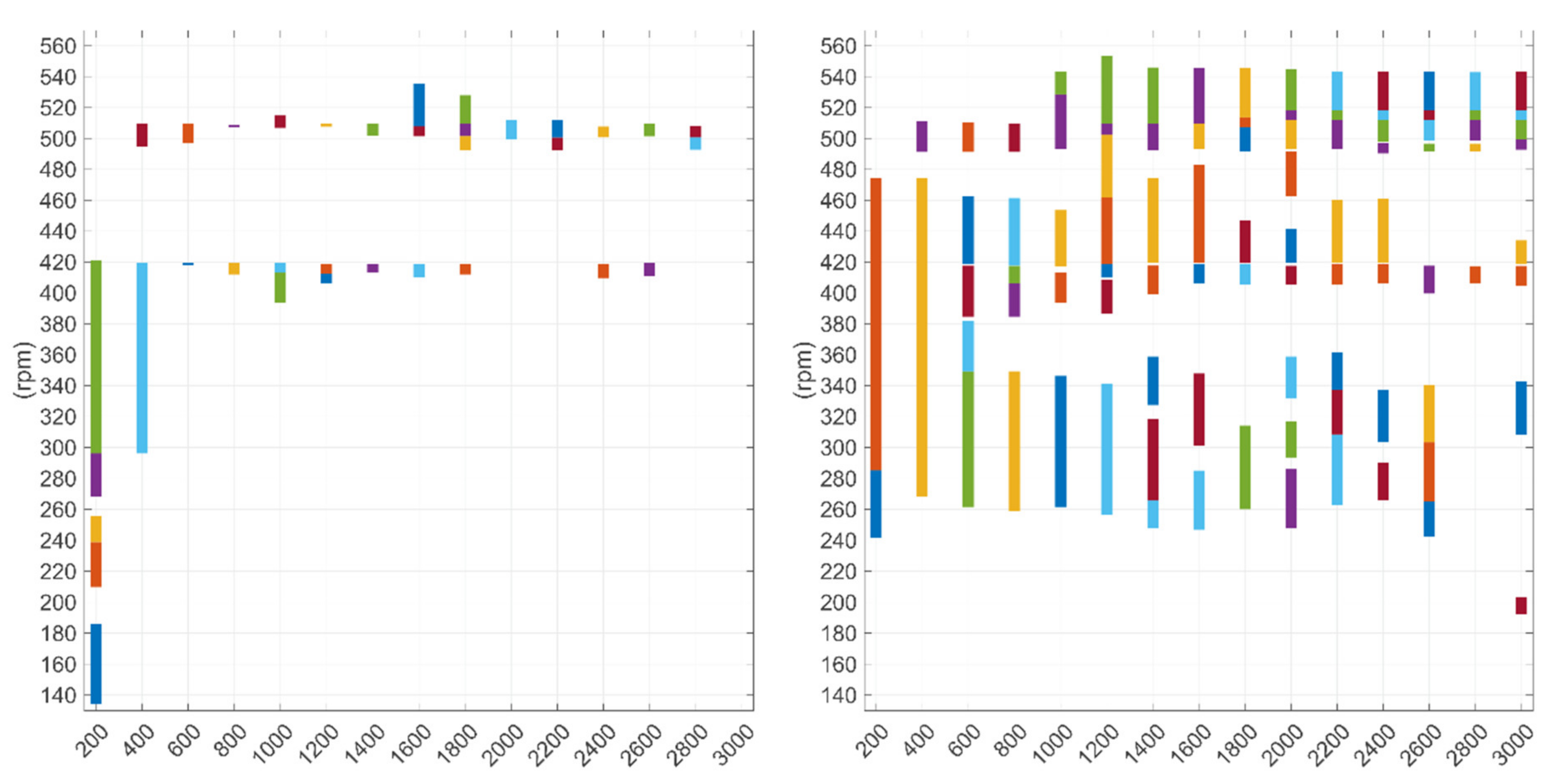
Figure 9 illustrates the shaft speed ranges that became selected for monitoring from the candidate subsets when all models (time-domain, bearing and gear) were identified together. Both plots show that the selected ranges were relatively wide when datasets were small, such as N = 200. When the datasets were larger, the selected ranges were typically narrower.
With the ‘basic training subsets’ approach (on the left), the highest number of selected subsets was five, in the case of N = 200. Then, the minimum number of samples in the subset could be as low as twenty (10% of N). Therefore, some of the subsets could be only faintly representative of the operation. When N was increased, areas around 410 and 500 rpm became selected, which could be explained by the frequent operation within such ranges (see Figure 4).
The plot on the right illustrates that generally a large proportion of the operating area was identified for monitoring irrespective of the sample size (N) when the ‘adaptive training subsets’ approach was used. The monitoring of a broad area is useful when the thruster is probably operated within a broad rotational speed range during typical use. The highest number of selected operating ranges for monitoring was nine in the case of N = 2000. When N = 200 or 400, only two ranges became selected. If many ranges are selected for use, multiple models and parameters must be identified, which may increase complexity. However, the use of simple models, as shown in Equation (1), helps to keep the complexity of the monitoring approach tolerable. Appendix C illustrates the ranges selected for the time-domain, bearing and gear models, when the models were identified separately from each other.
3.3. Effect of Training Data on Model Performance
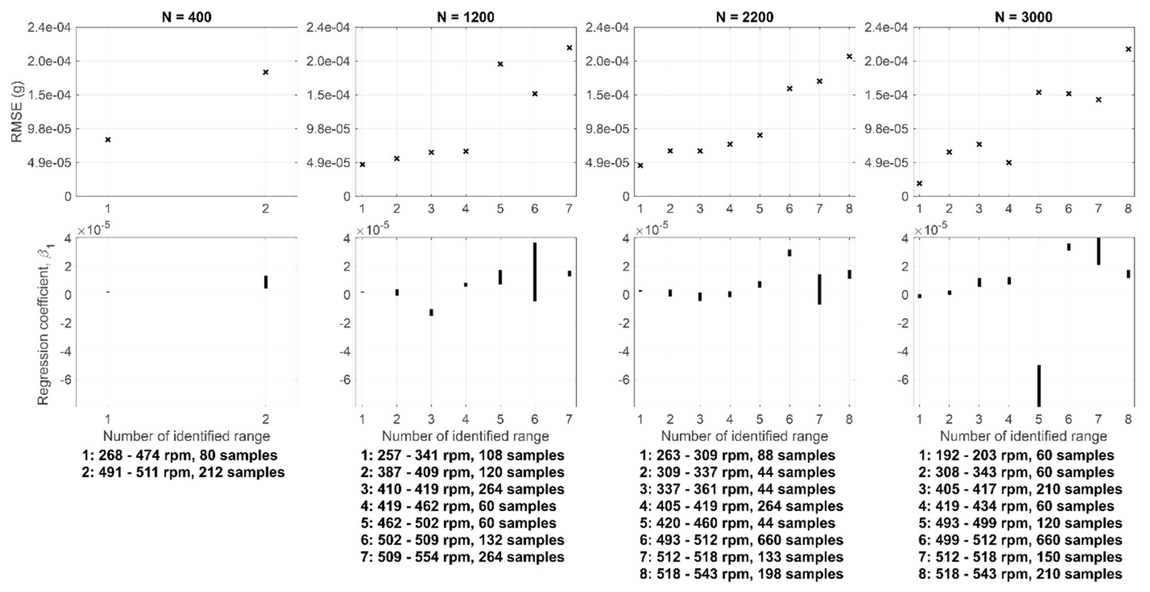
The upper plots in Figure 10 show the root-mean-square error (RMSE) for the linear regression in which GMF feature no. 1 was predicted by using the shaft speed values within different selected operating ranges. Models were identified by using the datasets with the sizes of 400, 1200, 2200 and 3000 samples. The selection of training subsets was conducted by using the ‘adaptive training subsets’ approach, where all the models were identified at the same time. Therefore, the presented models used the same operating ranges, as shown on the right in Figure 9.
The plots show that the modeling error was typically high when the speed range was selected from the higher end of distribution. This can be explained by the higher variation of values there, as shown by the plot on the lower left corner in Figure 7. However, such a correlation between RMSE and shaft speed cannot be generalized to every feature.
Moreover, the plots reveal that the number of samples within the selected speed ranges had only a minor effect on the modeling error. This is illustrated on the plots with different sample sizes (N) but similar speed ranges, such as range no. 2 on the plot with N = 400 and range no. 6 on the plot with N = 2200 with 212 and 660 samples within the ranges, respectively.
The lower plots in Figure 10 show the 95% confidence intervals for the regression coefficient (β1), see Equation (1). They were estimated based on the Wald test implemented in the coefCI function in MATLAB®. The plots reveal that the narrowest speed ranges (6–7 rpm wide) resulted in a high uncertainty of the regression coefficient values. However, this may be insignificant for monitoring purposes because the main idea in residual monitoring is to detect the increasing modeling error. At a narrow range, the predictor values vary only slightly. The plots also indicate that the number of samples within a range had no observable influence on the width of confidence intervals. A similar analysis was conducted for the intercept (β0), but due to the lack of additional value, it was omitted from here.
3.4. Computation Time in System Identification
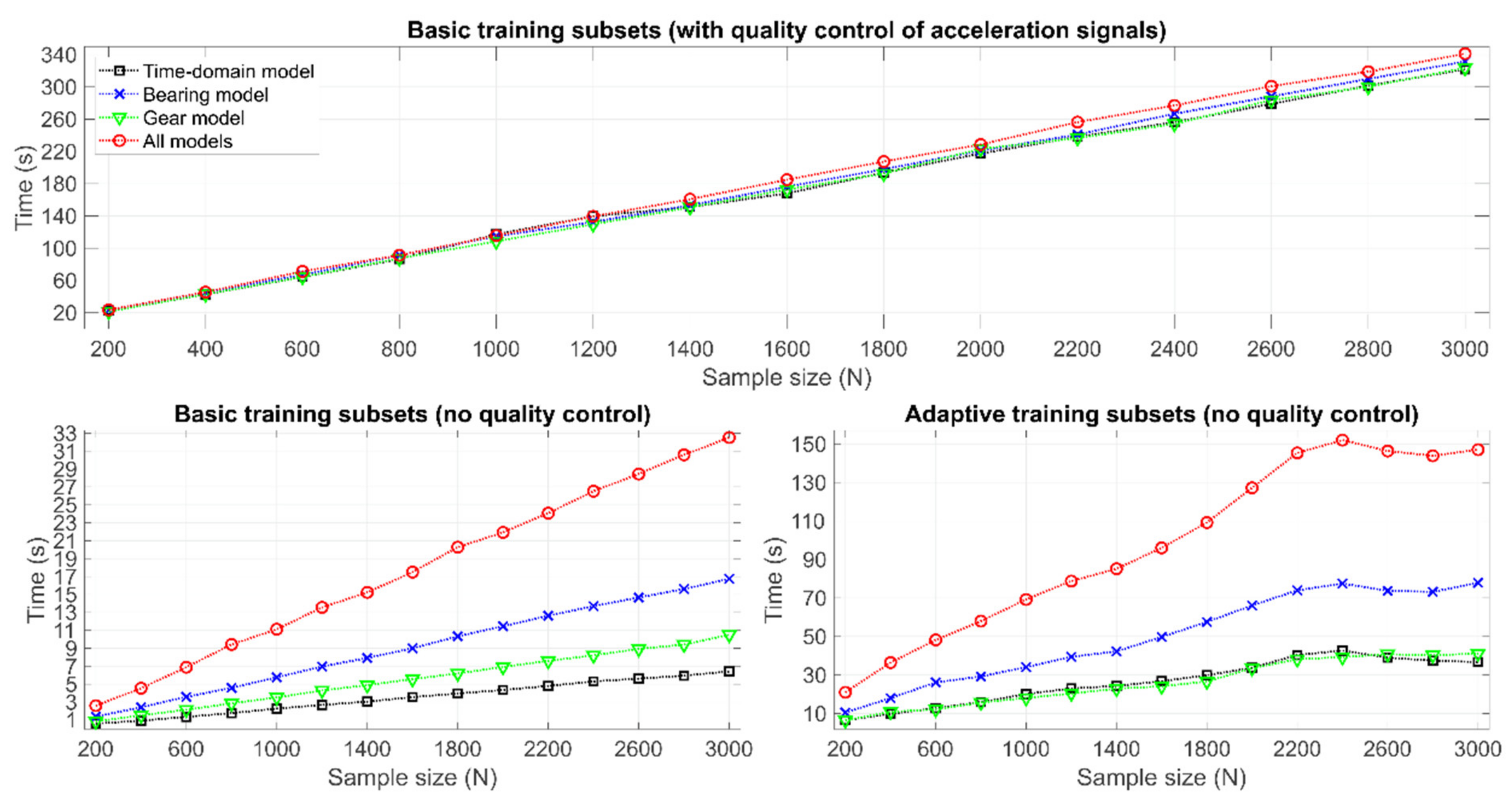
Figure 11 shows the computation time used in algorithm training as the average of two tests. The computations were performed with a standard office computer (2.20 GHz, Intel® Core™ i7-8750H CPU, 16.0 GB RAM) and MATLAB® R2020b. On the plot on top, the algorithm was trained with all its steps (see Figure 1) using the ‘basic training subsets’ approach. The plots below show the computation time without the quality control of samples, which means that each signal passed through the QC process without any processing.
The results show that the size of the sample set and computation time are strongly correlated. The larger the sample set was, the more time was needed. The same goes for the dimensionality of inputs. The algorithm with the bearing model required more computation than the algorithm with the gear model because the number of features was higher then. Comparing the plot on top with the plot below on the left, it becomes clear that QC consumed the most time in algorithm training. In QC, the most time was used by the check of moving mean range. The process was affected especially by the signal length, the window size and the motion of the window, which were 16,384; 100; and 1 value(s) here, respectively. To clarify further, the time used in quality control was independent of the approach to training subset selection (see Figure 1).
The computation time with the ‘adaptive training subsets’ approach appears low enough to be used in practice (with limited computing resources), which can be concluded from the results in the lower right plot in Figure 11. In addition, the plot reveals that the computation time was at a fixed level when N was 2200–3000 but the reason for that is unclear. However, the shape of the distribution is relatively stabilized with those datasets, as shown in Figure 5.
3.5. Comparison of Tests to Identify Normally Distributed Residuals
Figure 12 illustrates the percentage of normally distributed residual sets in training subset candidates based on five different hypothesis tests applied. The percentage values give an indication firstly on the adaptability of each hypothesis test to varying datasets and secondly on their usability in system identification. The ‘Adaptive training subsets’ approach was used in the tests, and therefore, the number of subset candidates varied in different datasets, as shown in Section 3.1. The residuals of all eleven features (see Table 1) were tested in each subset. Therefore, a 100% result requires a varying number of normally distributed residual sets in different datasets. In the case of N = 1000, for example, the number would be 11 × 4198 (the number of features × the number of training subset candidates).
In general, the results indicate that the number of normally distributed residual sets reduced when the sample size N grew. KS and AD results exhibit the highest percentages of normally distributed sets, which suggests they could be useful tests for practical implementation. Moreover, these methods had the largest change in percentage points when N changed, which indicates they have high adaptability to different datasets. The other tests, namely, Lilliefors’, JB and SW tests, resulted in lower percentages, indicating that the identification of suitable training subsets could be challenging if such tests were applied.
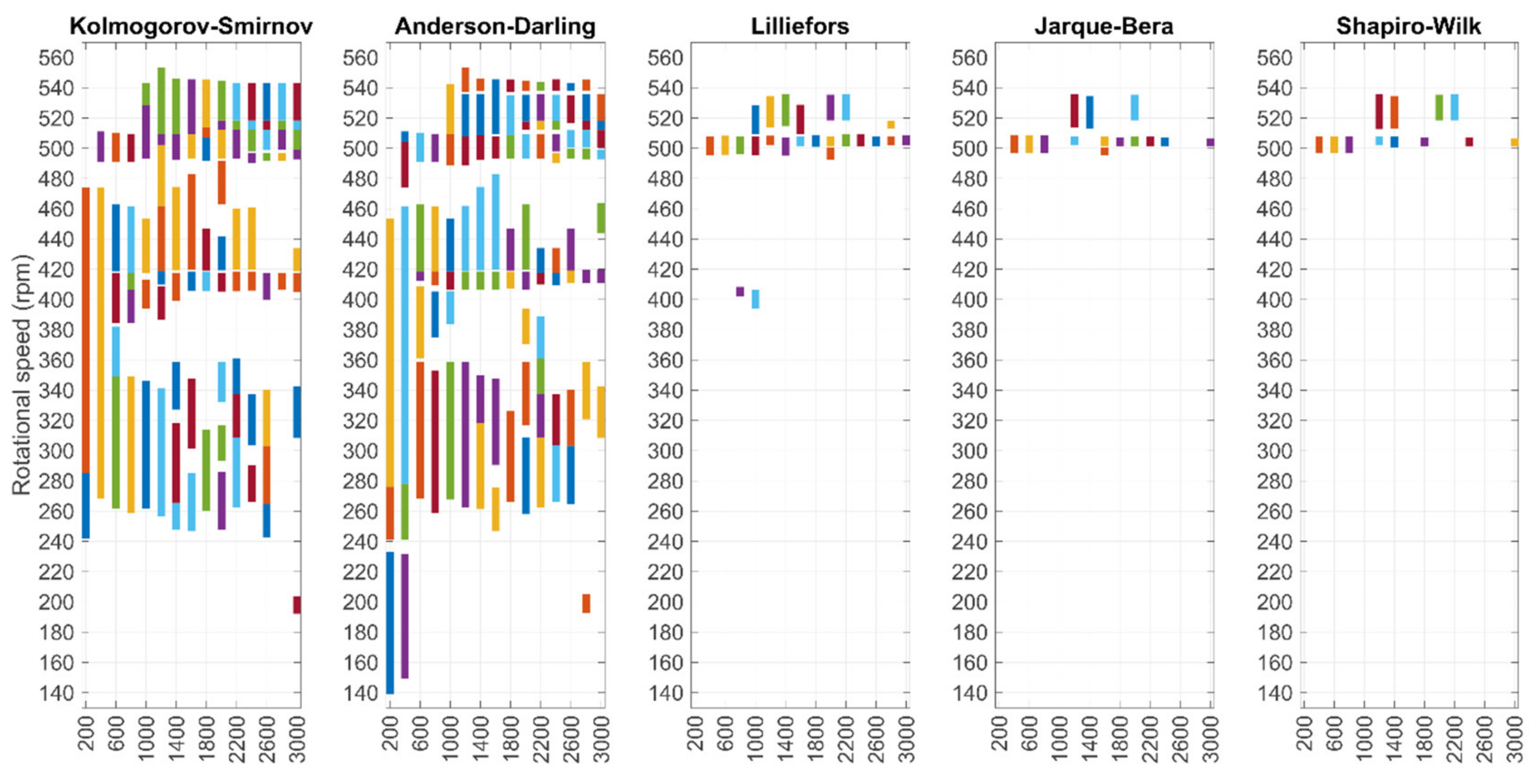
Figure 13 illustrates the operating ranges in the selected training subsets with different hypothesis tests. Relatively similar ranges with wide coverage were selected based on KS and AD. The other tests resulted in the selection of a low number of ranges. The ranges were narrow and mostly located at roughly 500 and 530 rpm speed. The selection of a few narrow ranges is unfavorable for practical monitoring.
The presented results are somewhat conflicting with the literature. Previously reported simulations reveal that powerful normality tests include methods such as SW or JB, whereas KS is less powerful [36,37]. By contrast, the results presented here suggest that the KS and AD tests could have high usability in the automated procedures presented, whereas SW and JB appear unfavorable. The selection of an appropriate test requires understanding of the considered application and its data.
4. Discussion
The results provide guidance to automated training subset selection in condition monitoring applications. Firstly, the results in Section 3.5 indicate that the broadest operating areas for monitoring could be identified by using the KS and AD tests for the check of residuals’ normal distribution. Secondly, the results in Section 3.2 and Section 3.5 show that the novel approach to dataset segmentation, namely, the ‘adaptive training subsets’ approach, adapts well to different training datasets. With this approach, usable training subsets were identified irrespective of dataset size and distribution. The results further indicate that the previously introduced approach, named here as ‘basic training subsets’, has limited usability on large datasets, but it could be used with small datasets or distributions which have a shape close to a uniform distribution.
The results show that the minimum width of a selected speed range should be constrained. The use of a narrow range is impractical for monitoring, unless the system is operated within the range regularly. The narrow range of the predictor variable, shaft rotational speed, results in wide confidence intervals for regression coefficients as shown in Figure 10. In such a case, a regression model may be useless unless it improves the normality of the samples used to define the multivariate normal distribution, which is the reference during monitoring, see [6]. In addition, the outlying samples from the edges of distribution should be omitted from the automated training subset selection, which was illustrated in Appendix C. A practical approach is to automatically select the operating areas for monitoring from a narrower interval, such as 1–99th percentiles, instead of the full distribution.
As shown in Figure 5 and Figure A1, every dataset collected from the monitored system was slightly different. The operation of azimuth thrusters, like many other industrial machines, is dynamic and the precise identification of the system based on a fixed training set is challenging. Therefore, it could be useful to update the models periodically based on the latest samples or by considering the samples from the earliest history to the current date, as was presented here, in Section 3. Such model maintenance, however, requires that the undamaged health state is ensured during the period covered by the training data, perhaps with additional methods. The versioning and control of files, databases, metadata and their relations require meticulous planning if the models are updated regularly. However, this should be feasible if the models are kept simple, as in Equation (1), and the number of features is low and their calculation is fast, as demonstrated in Section 3.4.
To further improve the training subset selection, it could be useful to study the shaft speed ranges where the deviation from the normal operation can be found the most effectively in the case of different faults. For example, the varying RMSE values in different speed ranges in Figure 10 illustrated that the level of change required for anomaly detection is varying. As illustrated in Figure 7, the typical variation of a vibration feature is sometimes larger on the high shaft speed (>400 rpm), and then, the absolute change in the feature value must be large to detect the anomaly. In some cases, it could be easier to detect the change in low-speed regions due to the lower typical variation in feature values, but the fault symptoms in low rotational speed may be faint [38]. Therefore, the research on signal processing to increase the sensitivity to varying faults could further benefit practical application and progress towards automated CM algorithms. Moreover, the ‘adaptive training subsets’ selection approach requires further testing on different applications to reveal its potential for the condition monitoring of rotating machines.
5. Conclusions
This study demonstrated the effects of training data size and distribution on automated training subset selection with a case study focusing on condition monitoring of azimuth thrusters based on a previously introduced algorithm and real measurement data. Two approaches to the segmentation of training data distribution were compared and five hypothesis tests for normal distribution were studied as a part of training subset selection. The selection of subsets was successful when the dataset was segmented flexibly into numerous subsets with varying sample sizes and ranges instead of using only a few subset candidates. The proposed ‘adaptive training subsets’ approach to dataset segmentation proved to be adaptable to all tested datasets exhibiting varying distributions and sizes. As a part of training subset selection, the normal distribution tests based on the empirical distribution functions, such as Kolmogorov–Smirnov or Anderson–Darling tests, were practical because a broad proportion of the entire operating area became covered in the training subsets. With the other hypothesis tests, the selected ranges were narrow and few. For the future development of automated condition monitoring, model training would benefit from research on sensitivity enhancement in fault detection and research on the reliability of data under the effects of varying operating situations.
Author Contributions
Conceptualization, R.-P.N.; methodology, R.-P.N.; software, R.-P.N.; validation, R.-P.N.; formal analysis, R.-P.N.; investigation, R.-P.N.; resources, S.A.B.; data curation, R.-P.N.; writing—original draft preparation, R.-P.N.; writing—review and editing, R.-P.N., M.R. and S.A.B.; visualization, R.-P.N.; supervision, M.R.; project administration, S.A.B. and R.-P.N.; funding acquisition, R.-P.N. and M.R. All authors have read and agreed to the published version of the manuscript.
Funding
This research was funded by Business Finland during Reboot IoT Factory project, grant number 4356/31/2019.
Institutional Review Board Statement
Not applicable.
Informed Consent Statement
Not applicable.
Data Availability Statement
Data sharing is not applicable to this article.
Acknowledgments
We thank the CMS team of Kongsberg Maritime Finland Oy and the project partners for the collaboration.
Conflicts of Interest
The authors declare no conflict of interest. The funders had no role in the design of the study; in the collection, analyses, or interpretation of data; in the writing of the manuscript, or in the decision to publish the results.
Appendix A
The distributions of the studied shaft speed values in the range 100–600 rpm are shown here as histograms with 20-rpm bar width.
Figure A1.
Distributions of rotational speed values in datasets of different sizes (N) shown as histograms with 20-rpm bin size. The vertical axes show the relative number of observations, i.e., the sum of all bar heights is equal to one.
Figure A1.
Distributions of rotational speed values in datasets of different sizes (N) shown as histograms with 20-rpm bin size. The vertical axes show the relative number of observations, i.e., the sum of all bar heights is equal to one.

Appendix B
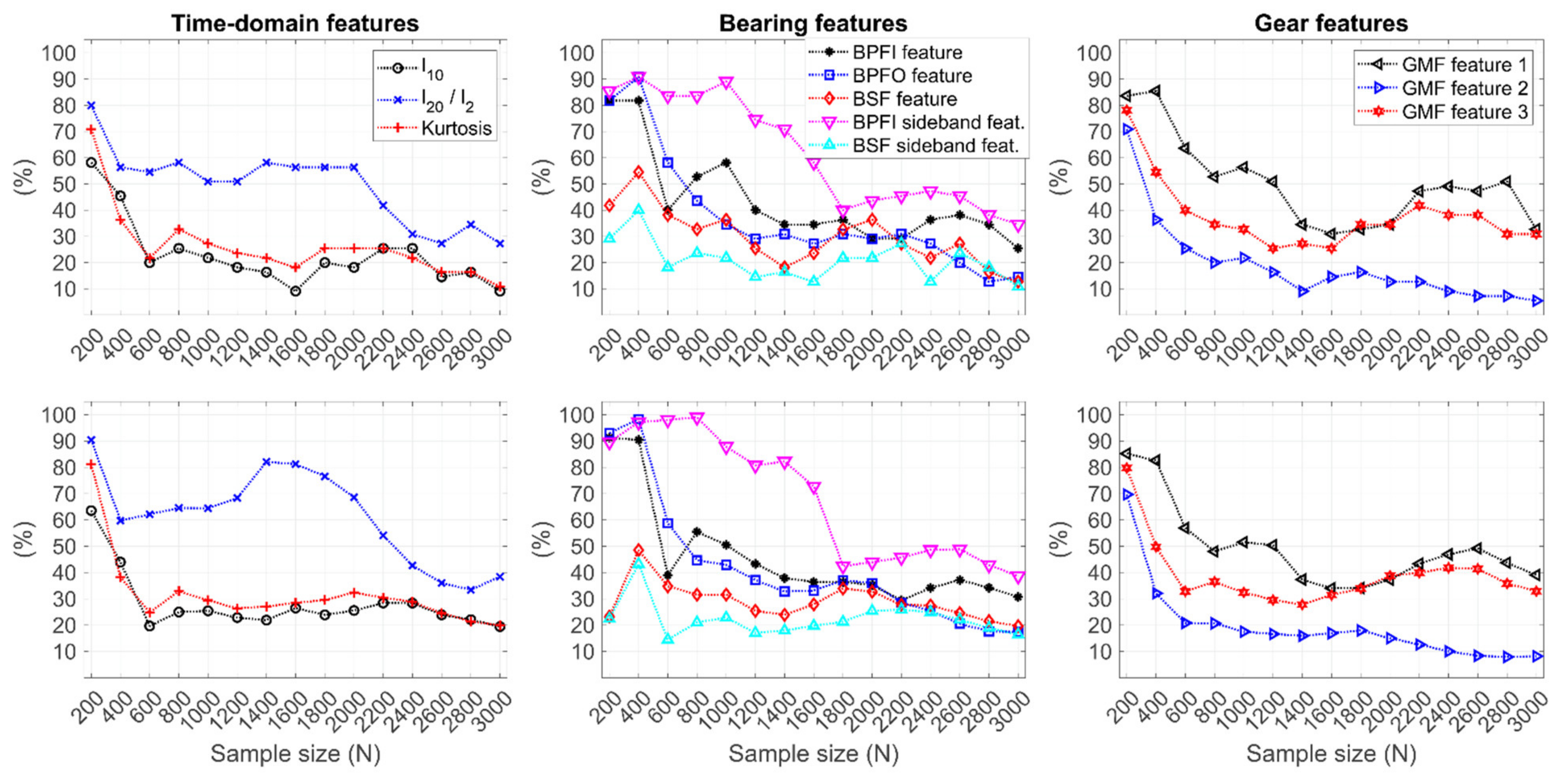
Figure A2 shows the percentage of acceptable training subsets for each feature individually. The results with the ‘basic training subsets’ approach are shown on top and the results with ‘adaptive training subsets’ are shown below. In general, the features with a low number of acceptable subsets limit the identification of appropriate models the most. In the time-domain model, l10 and kurtosis had the lowest percentages. Similarly, the BSF feature and BSF sideband feature had the lowest percentage with various sample sizes (N) in the case of bearing features. The most limiting feature for identifying the training subsets for the gear model was GMF feature no. 2.
Figure A2.
Percentage of acceptable training subsets for individual features. Dataset segmentation with ‘basic training subsets’ approach was used on top, whereas ‘adaptive training subsets’ approach was used below.
Figure A2.
Percentage of acceptable training subsets for individual features. Dataset segmentation with ‘basic training subsets’ approach was used on top, whereas ‘adaptive training subsets’ approach was used below.

Appendix C
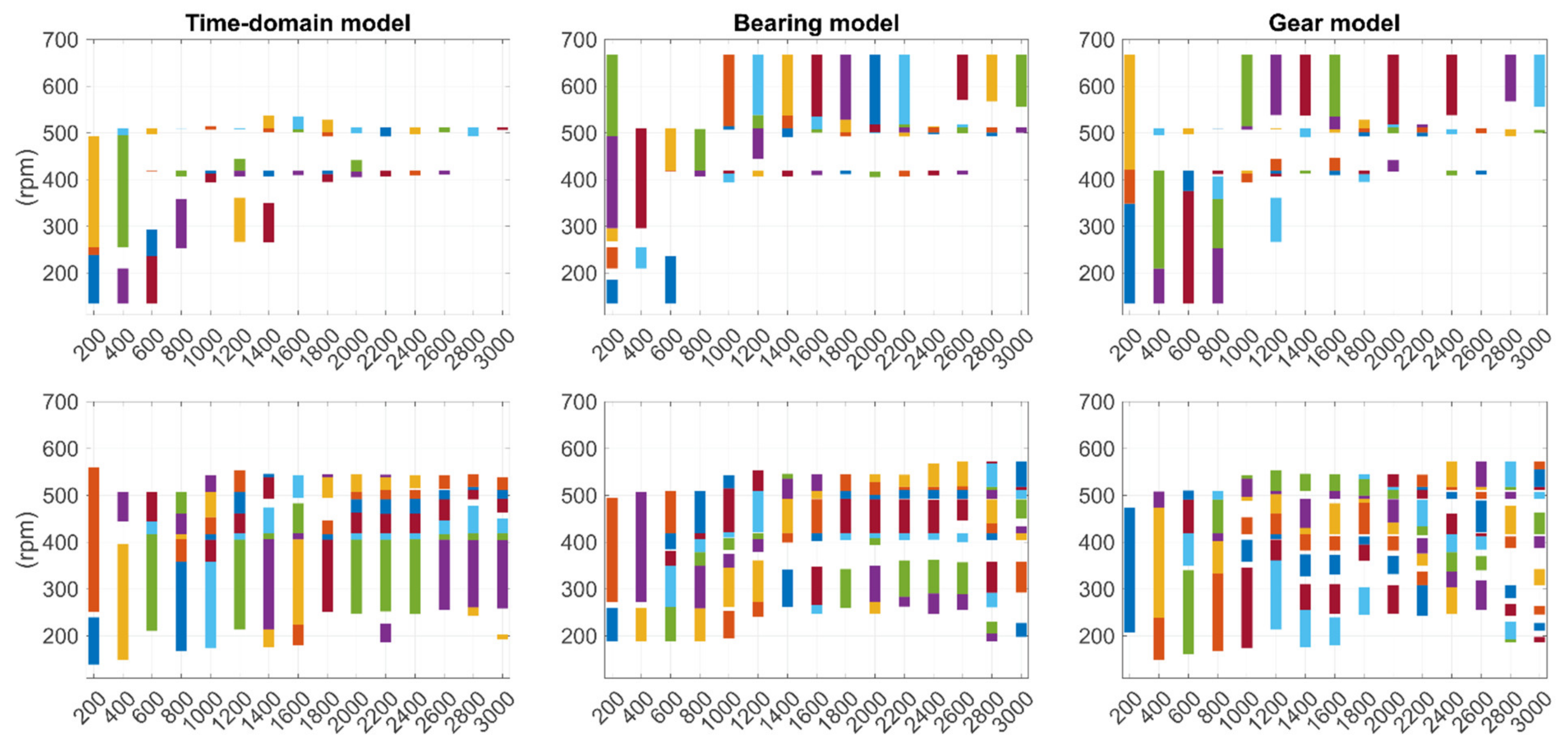
Figure A3 presents the shaft speed ranges selected for the time-domain model, the bearing model and the gear model when they were identified separately and with datasets of different sizes. The plots on top show the ranges selected with the ‘basic training subsets’ approach, whereas the ‘adaptive training subsets’ approach was used for the results illustrated on the plots below. In general, the operating ranges identified by ‘basic training subsets’ had low coverage of the total speed range in the datasets (see Figure 5). Moreover, ranges with relatively high shaft speed (up to 667 rpm) became selected with bearing and gear models from various datasets of size N ≥ 1000 samples. However, such ranges may not be representative because some high values in those datasets could be interpreted as outliers (see sample no. 115 with value 667 rpm in Figure 4). The extreme values of a dataset may require exclusion, as was conducted in the ‘adaptive training subsets’ approach. This approach also resulted in the identification of broad coverages for each model type and each dataset, as shown in Figure A3, which highlights its adaptive and reconfigurable properties in training data selection.
Figure A3.
Selected shaft speed ranges for different models. ‘Basic training subsets’ approach was used on top, whereas ‘adaptive training subsets’ was used below. Values on horizontal axis represent the sample size (N) and the vertical lines with different colors represent selected non-overlapping ranges.

References
- Sahal, R.; Breslin, J.G.; Ali, M.I. Big data and stream processing platforms for Industry 4.0 requirements mapping for a predictive maintenance use case. J. Manuf. Syst. 2020, 54, 138–151. [Google Scholar] [CrossRef]
- Marttonen-Arola, S.; Baglee, D.; Ylä-Kujala, A.; Sinkkonen, T.; Kärri, T. Modeling the wasted value of data in maintenance investments. J. Qual. Maint. Eng. 2022, 28, 213–232. [Google Scholar] [CrossRef]
- Lei, Y.; Yang, B.; Jiang, X.; Jia, F.; Li, N.; Nandi, A.K. Applications of machine learning to machine fault diagnosis: A review and roadmap. Mech. Syst. Signal Process. 2020, 138, 106587. [Google Scholar] [CrossRef]
- Wang, Z.; Liu, C. Wind turbine condition monitoring based on a novel multivariate state estimation technique. Measurement 2021, 168, 108388. [Google Scholar] [CrossRef]
- Santolamazza, A.; Dadi, D.; Introna, V. A data-mining approach for wind turbine fault detection based on SCADA data analysis using artificial neural networks. Energies 2021, 14, 1845. [Google Scholar]
- Nikula, R.-P.; Ruusunen, M.; Keski-Rahkonen, J.; Saarinen, L.; Fagerholm, F. Probabilistic condition monitoring of azimuth thrusters based on acceleration measurements. Machines 2021, 9, 39. [Google Scholar] [CrossRef]
- Piramuthu, S. Input data for decision trees. Expert Syst. Appl. 2008, 34, 1220–1226. [Google Scholar]
- Plutowski, M. Selecting Training Exemplars for Neural Network Learning. Ph.D. Thesis, University of California, San Diego, CA, USA, 1994. [Google Scholar]
- Sun, J.; Hong, G.S.; Wong, Y.S.; Rahman, M.; Wang, Z.G. Effective training data selection in tool condition monitoring system. Int. J. Mach. 2006, 46, 218–224. [Google Scholar] [CrossRef]
- García-Pedrajas, N. Evolutionary computation for training set selection. Wires. Data Min. Knowl. 2011, 1, 512–523. [Google Scholar] [CrossRef]
- LeCun, Y.; Bengio, Y.; Hinton, G. Deep learning. Nature 2015, 521, 436–444. [Google Scholar] [CrossRef]
- Kong, Z.; Tang, B.; Deng, L.; Wenyi, L.; Han, Y. Condition monitoring of wind turbines based on spatio-temporal fusion of SCADA data by convolutional neural networks and gated recurrent units. Renew. Energy 2020, 146, 760–768. [Google Scholar] [CrossRef]
- Kettaneh, N.; Berglund, A.; Wold, S. PCA and PLS with very large data sets. Comput. Stat. Data Anal. 2005, 48, 69–85. [Google Scholar] [CrossRef]
- Lv, Y.; Romero, C.; Yang, T.; Fang, F.; Liu, J. Typical condition library construction for the development of data-driven models in power plants. Appl. Therm. Eng. 2018, 143, 160–171. [Google Scholar] [CrossRef]
- Liu, R.; Yang, B.; Zio, E.; Chen, X. Artificial intelligence for fault diagnosis of rotating machinery: A review. Mech. Syst. Signal Process. 2018, 108, 33–47. [Google Scholar] [CrossRef]
- Karabadji, N.E.I.; Khelf, I.; Seridi, H.; Aridhi, S.; Remond, D.; Dhifli, W. A data sampling and attribute selection strategy for improving decision tree construction. Expert Syst. Appl. 2019, 129, 84–96. [Google Scholar] [CrossRef]
- Reeves, C.R. Training Set Selection in Neural Network Applications. In Artificial Neural Nets and Genetic Algorithms, Proceedings of the International Conference, Alès, France, 5 April 1995; Springer: Vienna, Austria, 1995; pp. 476–478. [Google Scholar]
- Dai, J.; Wang, J.; Huang, W.; Shi, J.; Zhu, Z. Machinery health monitoring based on unsupervised feature learning via generative adversarial networks. IEEE ASME Trans. Mechatron. 2020, 25, 2252–2263. [Google Scholar] [CrossRef]
- Leyva, E.; González, A.; Pérez, R. Three new instance selection methods based on local sets: A comparative study with several approaches from a bi-objective perspective. Pattern Recognit. 2015, 48, 1523–1537. [Google Scholar] [CrossRef]
- Alam, F.M.; McNaught, K.R.; Ringrose, T.J. A comparison of experimental designs in the development of a neural network simulation metamodel. Simul. Model. Pract. Theory 2004, 12, 559–578. [Google Scholar] [CrossRef]
- Niu, X.; Yang, C.; Wang, H.; Wang, Y. Investigation of ANN and SVM based on limited samples for performance and emissions prediction of a CRDI-assisted marine diesel engine. Appl. Therm. Eng. 2017, 111, 1353–1364. [Google Scholar] [CrossRef]
- Li, Y. Selecting training points for one-class support vector machines. Pattern Recognit. Lett. 2011, 32, 1517–1522. [Google Scholar] [CrossRef]
- Guo, G.; Zhang, J.-S. Reducing examples to accelerate support vector regression. Pattern Recognit. Lett. 2007, 28, 2173–2183. [Google Scholar] [CrossRef]
- Moreno-Torres, J.G.; Raeder, T.; Alaiz-Rodriguez, R.; Chawla, N.V.; Herrera, F. A unifying view on dataset shift in classification. Pattern Recognit. 2012, 45, 521–530. [Google Scholar] [CrossRef]
- Gama, J.; Žliobaite, I.; Bifet, A.; Pechenizkiy, M.; Bouchachia, A. A survey on concept drift adaptation. ACM Comput. Surv. 2014, 46, 1–37. [Google Scholar] [CrossRef]
- Zenisek, J.; Holzinger, F.; Affenzeller, M. Machine learning based concept drift detection for predictive maintenance. Comput. Ind. Eng. 2019, 137, 106031. [Google Scholar] [CrossRef]
- Kadlec, P.; Grbic, R.; Gabrys, B. Review of adaptation mechanisms for data-driven soft sensors. Comput. Chem. Eng. 2011, 35, 1–24. [Google Scholar] [CrossRef]
- Wei, D.; Han, T.; Chu, F.; Zuo, M.J. Weighted domain adaptation networks for machinery fault diagnosis. Mech. Syst. Signal Process. 2021, 158, 107744. [Google Scholar] [CrossRef]
- Massey, F.J. The Kolmogorov-Smirnov test for goodness of fit. J. Am. Stat. Assoc. 1951, 46, 68–78. [Google Scholar] [CrossRef]
- Anderson, T.W.; Darling, D.A. Asymptotic theory of certain “goodness-of-fit” criteria based on stochastic processes. Ann. Math. Stat. 1952, 23, 193–212. [Google Scholar] [CrossRef]
- Lilliefors, H.W. On the Kolmogorov-Smirnov test for normality with mean and variance unknown. J. Am. Stat. Assoc. 1967, 62, 399–402. [Google Scholar] [CrossRef]
- Jarque, C.M.; Bera, A.K. A test for normality observations and regression residuals. Int. Stat. Rev. 1987, 55, 163–172. [Google Scholar] [CrossRef]
- Shapiro, S.S.; Wilk, M.B. An analysis of variance test for normality (complete samples). Biometrika 1965, 52, 591–611. [Google Scholar] [CrossRef]
- Dufour, J.-M.; Farhat, A.; Gardiol, L.; Khalaf, L. Simulation-based finite sample normality tests in linear regressions. Econom. J. 1998, 1, C154–C173. [Google Scholar] [CrossRef] [Green Version]
- BenSaïda, A.; MATLAB Central File Exchange. Shapiro-Wilk and Shapiro-Francia Normality Tests. Available online: https://www.mathworks.com/matlabcentral/fileexchange/13964-shapiro-wilk-and-shapiro-francia-normality-tests (accessed on 22 September 2021).
- Adefisoye, J.; Golam Kibria, B.; George, F. Performances of several univariate tests of normality: An empirical study. J. Biom. Biostat. 2016, 7, 1–8. [Google Scholar]
- Saculinggan, M.; Balase, E.A. Empirical power comparison of goodness of fit tests for normality in the presence of outliers. J. Phys. Conf. Ser. 2013, 435, 012041. [Google Scholar] [CrossRef] [Green Version]
- Mishra, C.; Samantaray, A.K.; Chakraborty, G. Rolling element bearing fault diagnosis under slow speed operation using wavelet de-noising. Measurement 2017, 103, 77–86. [Google Scholar] [CrossRef]
Figure 1.
Flowchart for system identification with the position of ‘training subset selection’ highlighted (adapted from [6]).
Figure 1.
Flowchart for system identification with the position of ‘training subset selection’ highlighted (adapted from [6]).

Figure 2.
Candidates for monitored speed ranges based on two approaches to dataset segmentation, demonstrated with one training set (N = 3000): ‘Basic training subsets’ approach with 55 ranges is illustrated on top; ‘Adaptive training subsets’ approach with 4851 ranges is shown below.
Figure 2.
Candidates for monitored speed ranges based on two approaches to dataset segmentation, demonstrated with one training set (N = 3000): ‘Basic training subsets’ approach with 55 ranges is illustrated on top; ‘Adaptive training subsets’ approach with 4851 ranges is shown below.

Figure 3.
Drawing of UUC 455 thruster.

Figure 4.
Shaft speed values of samples in chronological order and the progression of distribution based on median, interquartile range and 95% coverage.
Figure 4.
Shaft speed values of samples in chronological order and the progression of distribution based on median, interquartile range and 95% coverage.

Figure 5.
Illustration of 1st to 99th percentiles of shaft speed values. The deciles from first to ninth are marked by using black lines with squares placed on chosen sample sizes.
Figure 5.
Illustration of 1st to 99th percentiles of shaft speed values. The deciles from first to ninth are marked by using black lines with squares placed on chosen sample sizes.

Figure 6.
Feature values and rotational speed in chronological order. The number of a sample is shown on horizontal axis, whereas vertical axis shows the value of each sample.
Figure 6.
Feature values and rotational speed in chronological order. The number of a sample is shown on horizontal axis, whereas vertical axis shows the value of each sample.

Figure 7.
Scatter plots between feature values and rotational speed using the largest training set with 3000 samples.
Figure 7.
Scatter plots between feature values and rotational speed using the largest training set with 3000 samples.

Figure 8.
Percentage of acceptable training subsets using different combinations of features. Dataset segmentation approach based on ‘basic training subsets’ on the left and ‘adaptive training subsets’ on the right.
Figure 8.
Percentage of acceptable training subsets using different combinations of features. Dataset segmentation approach based on ‘basic training subsets’ on the left and ‘adaptive training subsets’ on the right.

Figure 9.
Selected rotational speed ranges when all models were identified together. ‘Basic training subsets’ approach was used on the left, whereas ‘adaptive training subsets’ was used on the right. Values on horizontal axis represent the sample size (N) and the vertical lines with different colors represent selected non-overlapping ranges.

Figure 10.
Errors in prediction of GMF feature no. 1 using selected training subsets (above) and 95% confidence intervals of regression coefficient β1 (below). Number of samples in datasets increases on the plots from left to right. Selected shaft speed ranges from each dataset and number of samples within ranges are written below.

Figure 11.
Time used in algorithm training. Plot on top shows entire computation time when ‘basic training subsets’ approach was used. Plots below show corresponding computation time without quality control using ‘basic training subsets’ (left) and ‘adaptive training subsets’ (right). Note that vertical axes have different scales.

Figure 12.
Percentage of normally distributed residual sets based on five hypothesis tests. Results highlight the adaptation performance of the tests on different datasets as a part of the system identification procedure. Low percentage indicates poor applicability in practice.
Figure 12.
Percentage of normally distributed residual sets based on five hypothesis tests. Results highlight the adaptation performance of the tests on different datasets as a part of the system identification procedure. Low percentage indicates poor applicability in practice.

Figure 13.
Speed ranges in selected training subsets based on system identification with five different hypothesis tests applied. Values on horizontal axis represent the sample size (N) and the vertical lines with different colors represent selected non-overlapping ranges.
Figure 13.
Speed ranges in selected training subsets based on system identification with five different hypothesis tests applied. Values on horizontal axis represent the sample size (N) and the vertical lines with different colors represent selected non-overlapping ranges.


Table 1.
Description of features generated for condition monitoring.
| No. | Feature | Details |
|---|---|---|
| 1 | Generalized norm (l10) | Order of norm, p = 10 |
| 2 | Ratio of norms (l20/l2) | Ratio of high-order norm (p = 20) to low-order norm (p = 2) |
| 3 | Kurtosis | Indicator for the tails of probability distribution |
| 4 | BPFI feature | Median amplitude of 1–10 BPFI harmonics |
| 5 | BPFO feature | Median amplitude of 1–10 BPFO harmonics |
| 6 | BSF feature | Median amplitude of {1, 2, 4, 6} BSF harmonics |
| 7 | BPFI sideband feature | Median amplitude of the nearest sidebands on both sides of BPFI harmonics (20 sidebands altogether, spaced at shaft rotational frequency) |
| 8 | BSF sideband feature | Median amplitude of the nearest sidebands on both sides of BSF harmonics (8 sidebands altogether, spaced at FTF) |
| 9 | GMF feature 1 | Median amplitude of 1–4 GMF harmonics and two nearest sidebands on both sides (20 frequency components altogether) |
| 10 | GMF feature 2 | Median amplitude of 1 × GMF and two nearest sidebands on both sides (5 frequency components altogether) |
| 11 | GMF feature 3 | Median amplitude of 2 × GMF and two nearest sidebands on both sides (5 frequency components altogether) |
Table 2.
Applied parameter values in dataset segmentation approaches. Parameter N is the number of samples in complete training set.
Table 2.
Applied parameter values in dataset segmentation approaches. Parameter N is the number of samples in complete training set.
| Parameter | Basic Training Subsets | Adaptive Training Subsets |
|---|---|---|
| Number of subsets | 55 | ≤4851 |
| Distribution range in use (in percentiles) | 0–100 | 1–99 |
| Minimum range width (pp) | 10 | 1 |
| Minimum range width (rpm) | - | 5 |
| Minimum number of samples | 0.1 × N (rounded to integer) | 40 |
Publisher’s Note: MDPI stays neutral with regard to jurisdictional claims in published maps and institutional affiliations. |
© 2022 by the authors. Licensee MDPI, Basel, Switzerland. This article is an open access article distributed under the terms and conditions of the Creative Commons Attribution (CC BY) license (https://creativecommons.org/licenses/by/4.0/).
Share and Cite
MDPI and ACS Style
Nikula, R.-P.; Ruusunen, M.; Böhme, S.A. On Training Data Selection in Condition Monitoring Applications—Case Azimuth Thrusters. Appl. Sci. 2022, 12, 4024. https://doi.org/10.3390/app12084024
AMA Style
Nikula R-P, Ruusunen M, Böhme SA. On Training Data Selection in Condition Monitoring Applications—Case Azimuth Thrusters. Applied Sciences. 2022; 12(8):4024. https://doi.org/10.3390/app12084024
Chicago/Turabian StyleNikula, Riku-Pekka, Mika Ruusunen, and Stephan André Böhme. 2022. "On Training Data Selection in Condition Monitoring Applications—Case Azimuth Thrusters" Applied Sciences 12, no. 8: 4024. https://doi.org/10.3390/app12084024
Note that from the first issue of 2016, this journal uses article numbers instead of page numbers. See further details here.