


Abstract
Future income distribution will affect energy demand and its interactions with various societal priorities. Most future model simulations assume a single average consumer and thus miss this important demand determinant. We quantify long-term implications of alternative future income distributions for state-level residential energy demand, investment, greenhouse gas, and pollutant emission patterns in the United States (U.S.) by incorporating income quintiles into the residential energy sector of the Global Change Analysis Model with 50-state disaggregation. We find that if the income distribution within each U.S. state becomes more egalitarian than present, what means that the difference on income between the richest and poorest decreases over time, residential energy demand could be 10% (4%–14% across states) higher in 2100. This increase of residential energy demand will directly reduce energy poverty, with a very modest increment on economywide CO2 emissions (1%–2%). On the other hand, if U.S. states transition to a less equitable income distribution than present, with the difference between richest and poorest increasing over time, residential energy demand could be 19% (12%–26% across states) lower. While this study focuses on a single sector, we conclude that to improve understanding of synergies and tradeoffs across multiple societal goals such as energy access, emissions, and investments, future model simulations should explicitly consider subregional income distribution impacts.
Export citation and abstract BibTeX RIS
1. Introduction
Income inequality has increased substantially in the last 40 years in the U.S., making it one of the most unequal developed regions in the world [1]. Recent studies analyze the regressive nature of the energy system, showing that the energy burden of low-income households in the U.S. is three times greater than the burden of the higher income households [2–4]. Additionally, energy poverty has not been explicitly recognized in the U.S. as a problem separated from general poverty, what generates inefficiencies in the implementation of low-income programs aimed at combating energy poverty [5–7]. In this context, subregional income distribution could have a significant influence on energy demands, supplies, and emissions.
Literature shows that floorspace and residential energy demands are more income elastic at lower income levels and satiate at high income levels [8–12]. This implies that the response of floorspace and residential energy demands to a variation in income would be larger at lower than at higher income levels. For instance, even with very high income, people might not prefer additional rooms or larger houses [13]. Likewise, richer people might not prefer a room temperature of 50 °C during the winter [14], nor might they demand overly-bright lighting. Hence, if society transitions into a more egalitarian distribution in the future, in which the income difference between the richest and the poorest decreases over time for all the U.S. states (see section 2.2 for the details), lower income groups would experience faster and greater income growth with a resulting increase in residential energy demand [15]. In contrast, in an increasingly skewed income distribution scenario, much of the income would go to groups whose demands are already close to satiation. These changes in residential energy demand could have implications for a wide range of related metrics including energy consumption, investments, and greenhouse gas and air pollutant emissions [16].
Most previous studies incorporating income inequality considerations in their analyses are based on analysis of historical data [17–22] or use model projections, but without resolution in terms of specific end-use services [23, 24]. Table 1 shows a representative subset of key papers that explored income inequality and household energy demand in the last 30 years, while additional details on the literature review can be found in the SI (section 1 (available online at stacks.iop.org/ERL/17/014031/mmedia)).
Table 1. Summary of key papers analyzing the socio-economic dimensions of household energy use.
| Paper | Geographic scope | Period covered by analysis (historical or forward looking) | Demographic elements of focus | Type of Analysis (historical data versus model-based simulations) | Model Type (Use NA for statistical analysis of data) | Outcome metrics analyzed |
|---|---|---|---|---|---|---|
| Allen and Edmonds [25] | USA | Historical data and projections (1975,1978,1980–1990/2000) | Age, immigration status | Analysis of data and reported projections | NA | Growth of GNP |
| O'Neill & Chen [22] | USA | Historical data (1993–94) with cited projections to 2050/2100 | Household size, age | Statistical analysis of historical data | NA | Household energy use |
| Rausch et al [23, 26] | USA | Static model simulations on 2006 base year | (a) income class, region (b) Income, race/ethnicity, region of origin | Model-based projections | Multi-sector CGE (2011b with detailed hhold data for micro-simulation) | Welfare Impacts on full income (expenditure + factor income) from climate policy |
| Yanagisawa [18] | Japan | Historical data covering 2010–2015 | Income groups | Analysis of historical data | NA | Household energy consumption |
| Pachauri et al [27] | Developing Africa, South Asia | Projections over 2030 | Income groups, rural/urban | Model-based projections | Detailed, multi-sector energy model | Hhold energy consumption (of final fuels) |
| Andrich et al [20] | Australia | Historical 2011 data used for main analysis | Income groups | Calculation of key indicators from historical data | NA | Hhold income, CO2 emissions, water cons rates & health effects of emissions |
| Dennig et al [28] | Global (12 macro regions) | Projections to 2200 from model base year 2000 | Income groups | Model-based projections | Ramsey-type (simple, highly aggregate GE model), recursive dynamic | Climate impacts on per capita consumption |
| Cameron et al [29] | South Asia | Projections over 2050 | Income groups, rural/urban | Model-based projections | Detailed, multi-sector energy model | Hhold energy consumption (of final fuels) |
| Caron et al [30] | China | Projections to 2030 from model base year of 2007 | Income groups, urban/rural, regional location | Model-based projections | Multi-sector CGE | Household welfare impacts of climate policy |
| Reaños & Wölfing [19] | Germany | Hhold survey data for 2002 & 2012 | Income groups and household demographic breakdown | Econometric analysis of historical data | NA | Welfare impacts of heating cost changes |
| Khosla et al [31] | India | Historical data. 2017 (January and July) | Income groups | Econometric analysis of empirical surveys | NA | Energy demand, savings, and behavior |
| Dagnachew et al [32] | Ethiopia | Projections over 2030 | Income groups, rural/urban | Model-based projections | Detailed, multi-sector energy model with global IAM | Aggregate final energy consumption, emissions and investment |
| Oswald et al [17] | Global (86 countries) | Historical GTAP data for 2011 | Income | Calculation of key indicators from historical data | NA | Energy footprints, energy intensity and inequality |
In addition, forward-looking studies and particularly those derived using integrated assessment models, used to inform long-term strategic planning, have largely ignored the heterogenous nature of consumer demand [33–35], typically assuming a single representative consumer. Depending on how subregional income distribution patterns unfold into the future, the assumption of a single representative consumer could result in an under- or over-estimation of residential energy demand. In this study we use an innovative modeling framework to explore the long-term implications of alternative future income distributions for the residential energy sector, one of the most important demand sectors in many international energy assessments [34, 36], which accounted for 20% of total energy consumption in the U.S. in 2020 [37]. We use a version of the Global Change Analysis Model with state-level disaggregation for the U.S. (GCAM-USA), and we expand the representation of residential energy demand to include multiple representative consumers (income quintiles), each with a distinct income pathway within each of the 50 states. While this enhanced model has some limitations in terms of land-use dynamics or resolution of the consumer heterogeneity, we present an innovative approach to estimate the differences in residential energy demand for different consumer groups (quintiles) for alternative income distribution scenarios, and the associated system-wide implications for the energy and emissions systems. Additionally, this study is the first to conduct a forward-looking integrated analysis of the impacts of alternative income distributions at subnational scale.
We demonstrate that incorporating income distribution considerations has direct implications for long-term projections of residential energy demand, with subsequent effects on direct and indirect greenhouse gas (GHG) and air pollutant emissions, and power sector investments. We find that if U.S. states transition to a more egalitarian distribution, by 2100 it could result in 10% higher residential energy demand compared to a scenario in which current inequality patterns remain unchanged. This increase in demand has very little effect on system-wide emissions (1%–2%), although it can generate some modest tradeoffs for residential sector emissions and power sector investments. The effects of transitioning to a more egalitarian distribution on residential energy demands and emissions vary widely across states with the most prominent increases occurring in the Southwest, which are currently more unequal. In contrast, under a transition to a more skewed distribution, in which the wealthier income groups' incomes rise at a faster rate than lower income groups, residential energy demands, residential sector CO2 emissions, and power-sector investments could respectively be 19%, 18%, and 14% lower. In the context of the sustainable development goals [38] (SDGs), our results highlight that reducing inequality (SDG10) [39] would result in higher energy access (SDG7) [29, 40, 41], reducing energy poverty, with little effect on economywide emissions (SDG13) [42]. On the other side, it could generate some moderate tradeoffs for household air pollution (SDG3) [43] and power sector investments (SDG9) [44], which should be considered in long-term energy planning.
2. Methodology
2.1. Global Change Analysis Model (GCAM)
For this study, we use the GCAM with greater spatial detail in the U.S. region, referred to as GCAM-USA [45, 46]. This version of the model disaggregates the U.S into 51 subregions (50 states and District of Columbia) and works within the global GCAM modeling framework. The model explores human and Earth-system interconnections and is designed to explore how these evolve over time under the influence of critical socio-economic and bio-physical driving forces that can be modified according to different 'what-if' types of scenarios. The recursive-dynamic projections of GCAM are simulated in a way that consistently resolves interactions between the energy, economy, land, water, and climate systems within a fully integrated computational system. GCAM-USA is an open-source model and can be downloaded from an online repository. In this work, we use version 5.2 of GCAM-USA, which we further modified in ways that are explained below.
As a relevant feature for this study, we focus on the energy system, and in particular, the residential sector [47–49], while still maintaining the close integration with the other human and physical systems mentioned above. The building sector in GCAM-USA is disaggregated into 'residential' and 'commercial' sub-sectors. The floorspace demand is driven by population and income, so more (and/or richer) people will demand more floorspace until a satiation level is achieved. Below this satiation point the marginal utility of floorspace is positive. Above that point, the marginal utility is negative. The floorspace demand function in GCAM-USA is based on the formulation by Isaac and Van Vuuren [50], which has been extensively applied within integrated assessment modeling frameworks. It is summarized in the following equation
So, the per capita floorspace ( f) in region r, period t, and quintile i is determined by the exogenously defined satiation level (s), per capita income (I), and a time-invariant calibration-shape parameter ( ; 'satiation impedance') that represents the 'unobservable' effects driven by the variables that are not covered by the model. The details on these parameters can be found in the Supplementary information (SI, section 3.1.1), which also includes the link to the open-access GitHub repository with detailed model documentation. Total floorspace (
 ) will be calculated as per capita floorspace (
 ; see equation (1)) multiplied by population.
GCAM-USA models 14 residential services, namely cooling, heating, cooking, lighting, water heating, clothes dryer, clothes washer, computers, dishwashers, freezers, furnace fans, refrigerators, televisions, and other energy services. Cooling and heating are classified as thermal services while the other services are considered non-thermal. Demand for building services (per unit of floorspace area) depends on heating and cooling degree days, building shell conductivity, income, and satiation levels. The model also assumes satiation levels for service demands. This is summarized in the following equation (the sub-index for each service has been omitted for overview purposes):
where d is the service demand per unit of floorspace area in region r, period t and quintile i, k is a calibration parameter, DD is degree days, η is the exogenous average building shell conductance (see SI, section 3.1.2), R is the exogenous average floor-to-surface ratio of buildings (fixed to 5.5), IG is the internal gain heat from other building services, λ is an exogenous scale parameter that acts upon internal gains,  is a calibration-shape parameter ('satiation impedance'), I is the per capita income and P the price of the service. Note that for non-thermal services,
  = 1. Total service demand for each region, period, and quintile (
 ) will be calculated as service per unit of floorspace (
 ) multiplied by total floorspace (
 ).
).
The energy competition between fuels and technologies follows a logit choice model [51, 52] that prevents a winner-take-all response. So, parameters such as the fuel (endogenous) and non-fuel costs, share-weights, and the logit-exponents will have direct implications in the fuel-technology choice. The model has high-resolution details for energy services, incorporating different energy sources and/or technological options for producing each service. Additionally, the model assumes different pathways for the energy efficiency of each fuel-technology combination. Within each fuel, we explicitly model 'regular' and 'hi-efficiency' ('hi-eff') technologies where applicable. All the sector-fuel-technologies covered by the model are summarized in table S2. In terms of emissions, GCAM-USA estimates the emissions of CO2 at state, sector, and technology level for each period.
The main methodological innovation of this study is the incorporation of income quintiles to the residential sector. Each income quintile ( represents 20% of the population (fixed for all the scenarios and periods) and they are ordered from poorer (Q1) to richer (Q5). These quintiles are treated as distinct consumers in the residential energy sector and evolve over time as GCAM-USA is simulated forward and respond to income and price changes in ways defined by the demand functions discussed above. The SI (section 3.2) includes a detailed description on how these quintiles have been constructed and incorporated into the model. Finally, the calibration year of the version of the model used in this study has been updated to 2015 instead of 2010, which is the final calibration year in the default GCAM-USA version (v5.2). This upgrade enables us to more accurately calibrate our floorspace and service demand functions to recent history. Figure 1 summarizes the model structure and highlights the methodological innovations developed for this study.
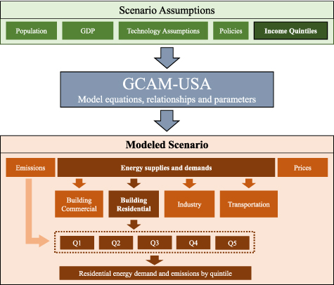
Figure 1. Overview of the methodology. The darker colors represent the modeling capabilities developed for this study.
Download figure:
Standard image High-resolution imageWe note that GCAM-USA does not include details on the household market, so the price effect is not captured by the model. GCAM-USA is not designed to include the full representation of households, so there are some variables, such as the household members or occupancy profiles that are not captured and would have some effect on our results [53]. Likewise, our floorspace function currently does not include vintage dynamics of the building sector (e.g. age structure of buildings, and capital stock turnover). In addition, floorspace is not linked with land-use in the model, so it does not capture the potential effects on land use change emissions of shifting industrial or agricultural into residential land. Nevertheless, the effects and preferences that are not covered by the variables in the model, are captured by the calibration parameter ( ), which corrects the difference between the observed and the estimated values in the final calibration year. To represent these fixed unobservable effects, this calibration parameter is kept invariant during the whole time-horizon. We note that, recent work has compared our building energy projections against a more sophisticated and detailed buildings model and found that future residential energy projections would be consistent across the models [54].
2.2. Income distribution scenarios
We introduce three illustrative scenarios for the U.S. that vary across assumptions about future income distributions. Our reference scenario is the 'Constant Income Distribution' scenario (hereinafter Constant), where income distributions remain constant at 2015 proportions throughout the century. We then construct the 'More Egalitarian Income Distribution' scenario (Egalitarian) in which all the states transition to the current income distribution of the most equal country in the world (Slovenia) in 2100. We note that the country with the narrowest gap across income quintiles is the one that we refer to as the most 'equal'. In this scenario, lower income quintiles become relatively wealthier while upper quintiles see a modest decrease in income share compared to the Constant scenario. Our third scenario, namely, 'More Skewed Income Distribution' (Skewed) assumes that all states transition to the current income distribution of the most unequal country in the world (South Africa) in 2100. In this scenario, only the income share of the wealthiest quintile increases relative to the Constant case, while the income shares for the four lower quintiles decrease compared to the Constant scenario. These scenarios are summarized in table 2, and more information can be found in SI (section 3.3, figure S5).
Table 2. Income distribution scenarios explored in this study.
| Scenario | Short name | Description |
|---|---|---|
| Constant income distribution | Constant | Income distributions are kept fixed at 2015 levels through 2100. These vary by state, with Gini coefficients a ranging from 0.37 to 0.47. |
| More egalitarian income distribution | Egalitarian | All states transition to the current income distribution of the most equal country in the world (Slovenia) in 2100, with a Gini coefficient of 0.25. |
| More skewed income distribution | Skewed | All states transition to the current income distribution of the most inequal country in the world (South Africa) in 2100, with a Gini coefficient of 0.63. |
aThe Gini coefficient is an index to measure income inequality of a determined population group (U.S. states in this study). The Gini coefficient is calculated as the area below the Lorenz curve (L(x)), a function that represents the relation between the cumulative income and the cumulative population. Mathematically,  , so a Gini coefficient of 0 indicates perfect equality and a Gini of 1 indicates perfect inequality. Therefore, a lower Gini coefficient means a more equal population.
We note that the above scenarios are purely illustrative, so the transition to the egalitarian and skewed distributions is not symmetric. While actual distributions might evolve differently into the future, these scenarios are designed to be simple 'what-ifs' based on observed outcomes. In addition, we acknowledge that the income distributions in 2100 may not be bounded to today's extremes. However, given the large uncertainty in how income distributions might evolve over a century-scale timeframe, the scenarios have been designed to lie at the boundaries of what is observable.
We also note that population and average income of each state increase over time following central estimates in existing literature [37, 55, 56]. These trajectories are equal for the three analyzed scenarios. This helps us ensure that the effects across scenarios are exclusively due to changes in the income distribution. For example, we assume that population in California grows from 39 M in 2015 to 57 M in 2100. Similarly, average per capita income grows from 40 to 118 thousand dollars per person (Thous$/pers). Then, differences across scenarios are exclusively driven by share of the income allocated to each quintile during the analyzed time horizon. While the central scenarios follow the 'business-as-usual' conditions and central estimates for the socioeconomic narrative, additional scenarios which include alternative socioeconomic pathways, modeling assumptions, and the transition to a low carbon economy have been explored in a sensitivity analysis (section 3.3).
Finally, the focus of our analysis is on a century-scale timeframe. While this long-term perspective is important in the context of CO2 emissions and power-sector investments [57], we present results for the 2050 timeframe in the SI (figures S14–S16).
3. Results
3.1. National floorspace and residential energy demands
Demands for per capita floorspace and residential energy services (e.g. cooling, heating, water heating, lighting, etc) increase over time in the Constant scenario in response to increasing per capita income. Considering that average income and population increase over time in all scenarios, floorspace in 2100 accounts for 38 billion square meters (billion m2) in the Constant scenario- an increase of 107% relative to 2015 (figure S7). Similarly, residential energy demand increases by 86% in the same periods, achieving around 20 EJ in 2100 (figure S8).
Changes in the income levels of different consumers (classified as income quintiles) driven by the transition to alternative income distributions entail variations in both floorspace and residential energy demands. In the Egalitarian scenario, floorspace and residential energy demands in 2100 are 11% and 10% higher compared to the Constant scenario (figure 2). This is because, as income shifts from upper to lower quintiles, the rise in demand for floorspace and energy by the lower (less satiated) quintiles is greater than the decline in demand for floorspace and energy by the upper (and more satiated) income groups. In contrast, floorspace and residential energy demands in 2100 are 15% and 19% lower in the Skewed scenario than in the Constant scenario. In the Skewed scenario, lower quintiles are relatively poorer and upper quintiles are relatively richer (compared to the Constant scenario). In fact, only the wealthiest quintile (Q5) is relatively richer in the Skewed scenario compared to the Constant scenario (figure S5). Hence, lower quintiles have lower floorspace and energy demands. Since the wealthiest quintile is already closer to satiation, the higher income in this scenario results in modest increases in floorspace and energy demands (+0.6% and +5%). Aggregated floorspace and residential energy demands in the Skewed scenario are lower than in the Constant scenario. Most of the changes in residential energy demand due to the transitions to alternative income distributions translate into changes in electricity and gas use (SI, figures S10 and S11). However, the transitions do not significantly affect the fuel composition of the residential sector—that is, the relative shares of the fuels remain almost unchanged (SI, section 4.2). These changes in floorspace and residential energy demands have little impact on aggregated system-wide CO2 emissions.
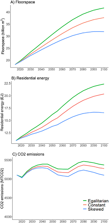
Figure 2. Floorspace, residential energy demand, and CO2 emissions in the U.S. by period and scenario. (A) Total floorspace (billion m2). (B) Total final energy in the residential sector (EJ). (C) System-wide CO2 emissions (MTCO2). The description of the Constant (Constant Income Distribution), Egalitarian (More Egalitarian Income Distribution), and the Skewed (More Skewed Income Distribution) scenarios can be found in table 2.
Download figure:
Standard image High-resolution imageSubstantial differences in energy demands by service exist across quintiles and scenarios. In the Constant scenario, all quintiles increase their total residential energy consumption by 2100 due to the over-time increase in population and floorspace demand (figure 3, top row). In the Egalitarian scenario, the lower quintiles increase their energy demand for all services (including thermal and non-thermal) as they become relatively richer, compared to Constant (figure 3, central row). In the Skewed scenario, consumers in the wealthiest quintile (Q5) have achieved the satiation level for thermal services (heating and cooling; figure 3, bottom row). Hence, with relatively higher income in this scenario, the demands of the wealthiest quintile for these services hardly increase (+2.3% and +1.5% respectively). However, the demand for non-thermal services (e.g. appliances, water heating, lighting, cooking, or electronic devices) increases more substantially (+8%).
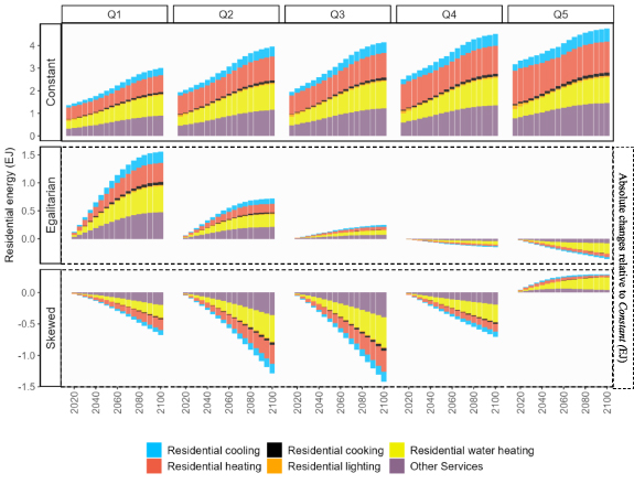
Figure 3. Residential energy by service in the Constant scenario and differences when transitioning to alternative income distributions (Egalitarian and Skewed), by sector, period, quintile, and scenario (EJ). Other services include the sum of clothes dryer, clothes washer, computers, dishwashers, freezers, furnace fans, refrigerators, televisions, and other energy services. The detail of these sectors is presented in section 3.5 in the SI. The description of the Constant (Constant Income Distribution), Egalitarian (More Egalitarian Income Distribution), and the Skewed (More Skewed Income Distribution) scenarios can be found in table 2.
Download figure:
Standard image High-resolution image3.2. Subnational dynamics
The evolution of per capita floorspace, total floorspace, and the residential energy demand have significant divergences across the U.S. states. Northern states, such as Minnesota or Vermont, have the highest per capita floorspace values in 2100 in the Constant scenario, as they have less urbanized areas and highest initial values (figure 4 top row). However, the most populated states, namely California, Texas, Florida, and New York show the highest values for absolute floorspace and residential energy demand, in base years, and in 2100.
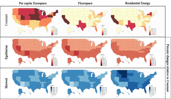
Figure 4. Per capita floor space, total floor space, and total residential energy in 2100 by state in the Constant scenario, and relative differences (%) in 2100 when transitioning to alternative income distributions. First row (shaded) shows the absolute values in 2100. Second and third rows show the percent change in 2100 for each variable when transitioning to the either Egalitarian or Skewed scenario, respectively. Red corresponds to increase relative to Constant scenario and blue corresponds to decrease relative to Constant scenario. The description of the Constant (Constant Income Distribution), Egalitarian (More Egalitarian Income Distribution), and the Skewed (More Skewed Income Distribution) scenarios can be found in table 2.
Download figure:
Standard image High-resolution imageThe impacts of alternative income distributions are heterogeneous across the U.S. In the Egalitarian scenario, per capita floorspace, floorspace, and residential energy increase throughout the U.S, compared to the Constant scenario (figure 4 central row). Most of these increases occur in Southwestern states (e.g. Nevada, New Mexico, and Arizona). These states are relatively more unequal in the base year (figure S3). Hence, the transition to a more egalitarian distribution results in higher increases in income for the lower income quintiles in these states compared to other states. In addition, the lower income quintiles in these states also have lower per capita floorspace and residential energy per unit floorspace in the base year, which implies more room for demand growth as income increases in this scenario. In the Skewed scenario, per capita floorspace, total floorspace, and residential energy decreases in all states in 2100, but the reductions are greater in the Northern states (e.g. Montana or Wyoming) which become relatively more unequal compared to the Constant scenario (figure 4 bottom row).
These changes in residential energy have some moderate impacts on total CO2 emissions (see figure 2(C)), mostly attributable to the residential sector (associated with the consumption of primary fuels), and the power sector (as a result of changes in residential electricity demand), with additional minor effects in other sectors due to indirect equilibrium effects. At U.S. level, the increase in energy consumption associated with the transition to the Egalitarian scenario, only increases economywide CO2 emissions by 1.8% in 2100, with different patterns across states (figure 5). Focusing on the residential sector (SI figure S12), the largest increases in residential CO2 emissions occur in California (+10%) and Southern and Eastern states such as Florida (+12%), Delaware (+11%), and New York (+10%), in which residential energy increases are the highest. In the Skewed scenario, 2100 residential CO2 emissions decrease relative to the Constant scenario due to lower residential energy demands. The largest reductions in the residential CO2 occur in Northern states such as Minnesota (−27%), Wyoming (−27%), Idaho (−26%), and Colorado (−24%) where decreases in residential energy demands are the highest.
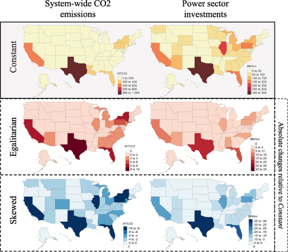
Figure 5. System-wide CO2 emissions in 2100 and undiscounted cumulative power sector investments (2020–2100) in the Constant scenario, and absolute differences when transitioning to alternative income distributions. First row (shaded) shows the absolute values. Second and third rows show the change for each variable when transitioning to the either Egalitarian or Skewed scenario, respectively. Red corresponds to an increase relative to Constant scenario and blue corresponds to decrease relative to Constant scenario. The description of the Constant (Constant Income Distribution), Egalitarian (More Egalitarian Income Distribution), and the Skewed (More Skewed Income Distribution) scenarios can be found in table 2.
Download figure:
Standard image High-resolution imageChanges in residential energy have implications for other GHG and air pollutant emissions as well but are also concentrated in the residential sector with little impact on system-wide emissions. For example, the increase in biomass and gas use in the residential sector associated with heating or non-thermal services (e.g. water heating) in the Egalitarian scenario results in an increase in carbon monoxide (CO), nitrogen oxides (NOx ), and non-methane volatile organic compounds emissions by 6%–7% in 2100 in the residential sector, while in the Skewed scenario, they are reduced between 15%–16% due to the reduction in residential energy (figure S13). Although the reductions are small, these changes in air pollutant emissions could have adverse implications for human health [58, 59]. Including income distribution effects in other sectors could potentially have more significant consequences (which we further elaborate upon in section 4—Discussion—later in the paper).
Furthermore, the higher electricity and energy demands result in a subsequent increase in power sector investments. In cumulative values (2020–2100), the investment needs associated with the power sector account for $3.26 trillion in the Constant scenario. The higher energy consumption in the Egalitarian scenario results in a national increase in investment needs of $0.2 trillion (+6%), over the base case. In absolute terms the highest investment increases are located in the largest states (Texas, California or Florida). However, in relative terms, the tradeoff is especially relevant in Southern states such as Florida, where investments increase around 10% compared to the Constant scenario. Conversely, the decrease in energy demand in the Skewed scenario reduces the cumulative power sector investments by around $0.5 trillion (−14%). Although the higher reductions occur in the most populated states, the largest relative reductions in power sector investments occur in Florida (−16% compared to Constant), followed by Alaska (−12%), Idaho (−12%), and New York (−11%).
3.3. Sensitivity analysis
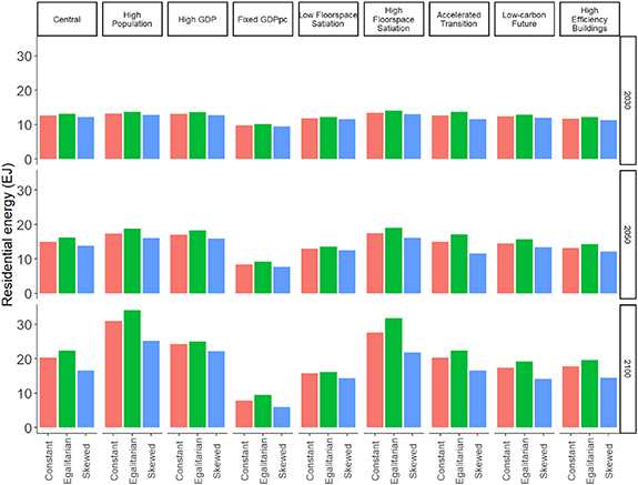
To explore the robustness of our findings, we conduct a sensitivity analysis on the following key factors: future population; future Gross Domestic Product (GDP) growth; the level of satiation in floor space demand; the assumed period for the transition of income distributions from the base levels to the scenario-specific target values; system-wide deployment of non-emitting technologies; and the deployment of energy efficiency measures in the residential sector (figure 6). Specifically, we run the following sensitivity scenarios (a) higher population; (b) higher GDP growth; (c) a scenario where population and GDP are fixed at 2015 levels ('Fixed GDPpc'); (d) lower and (e) higher floor space satiation levels compared to the central assumptions; (f) a transition to the egalitarian and skewed distributions by 2050 (as opposed to 2100 which is our central assumption); (g) a transition to a low-carbon economy; and (h) alternative building shell efficiency assumptions that combine a more ambitious efficiency improvement over time with an explicit differentiation by quintile. More details on the description of these sensitivity scenarios can be found in the SI (section 3.4).
Figure 6. Sensitivity analysis of the residential energy demands in the U.S. by period, sensitivity, and scenario. The panels show the residential energy demand by period under central and eight alternative assumptions namely High Population, High GDP, Fixed GDPpc, Low Satiation, High Satiation, Accelerated Transition (in which states are assumed to transition to the egalitarian and skewed distributions by 2050 instead of 2100 which is our central assumption), Low-carbon future, and High Efficiency Buildings. The description of the Constant (Constant Income Distribution), Egalitarian (More Egalitarian Income Distribution), and the Skewed (More Skewed Income Distribution) scenarios can be found in table 2. Detailed assumptions under the sensitivity cases are described in the SI, section 3.4.
Download figure:
Standard image High-resolution image
In all of the above sensitivity cases, residential energy demand increases in the Egalitarian case and decreases in the Skewed scenario (relative to the Constant scenario)—suggesting that the qualitative insights of our analysis are robust across different assumptions even if there are some quantitative differences. For example, the lower floor space satiation level assumption [50, 60] (60 m2/person as opposed to 100 m2/person in our central assumptions)—which is indicative of a transition toward a more urban lifestyle and compares with low energy demand scenarios reported in the literature [61]—results in lower residential energy demands in all scenarios, compared to the scenarios with central assumptions (100 m2/person). Under this assumption, all quintiles are closer to their satiation levels in the base year. Hence, changes in energy demands in the Egalitarian and Skewed scenarios compared with the Constant scenario are substantially moderated. With the lower satiation level, residential energy in 2100 increases by around 2.5% and decreases by around 9% under the Egalitarian and Skewed scenarios respectively compared to the Constant scenario.
4. Discussion
Our analysis shows that a society with lower income inequality could result in significantly improved energy access, reducing the current regressive behavior of the energy system, with very little effect on cumulative economywide CO2 emissions. This result is consistent with recent finding by various studies [32, 62–67]. We also find that the transition to a more egalitarian society could generate some moderate tradeoffs with other societal priorities or SDGs, such as an increment of CO2 and air pollutant emissions from the residential sector, or a requirement for some additional investments in the power sector, as pointed by different studies [15, 68–72]. However, these adverse side-effects could be ameliorated if the more equal income distribution is combined with a limited use of fossil fuels, or a more rapid adoption of more efficient and/or cleaner technologies and building shells by households.
Broadly, this work demonstrates that incorporating heterogeneity in terms of consumers could have important implications in shaping our understanding of future residential energy demand and emissions. Our results suggest that assuming a single representative consumer could result in under- or over-estimation of demands depending on how income distributions evolve into the future (SI, Section 8). These results are aligned with the emerging scientific literature that analyzes the importance of systematically considering not only international inequality but subregional income distribution pathways in the context of global scenario analysis [73–75]. Our results directly contribute to this research agenda, since, to our knowledge, this is the first study that uses a subregional scale (U.S.-state level) to explore forward-looking implications of alternative income distributions for residential energy demand and the associated effects for emissions and power sector investments. In addition, another novel aspect of the study is the development of a sensitivity analysis that shows that the obtained qualitative insights are robust to different uncertain assumptions on the building sector (such as satiation level or the shell efficiency projections), the socioeconomic narrative, and the underlying climate strategy. The consistency of our qualitative insights across a wide range of alternative futures should be of interest for regional and national policymakers.
We note that the degree of synergy and tradeoff across multiple societal priorities would also be affected by a range of factors that were not considered explicitly in this study such as the future evolution of lifestyles and cultural traditions [61, 76], and the implementation of air quality measures. Future work might account for these factors in more detail. More broadly, while the qualitative insights of this study might be generalizable to countries beyond the U.S., the quantitative results are more representative for developed economies and care must be taken in extrapolating our results to the rest of the world. For instance, there are significant differences in the demand for floorspace across regions around the world [47, 50, 60], with less-developed regions being far from the assumptions used in this study [77]. Similarly, in our U.S.-focused study, most of the increased energy demand in the Egalitarian scenario is accounted for by an increase in electricity and gas use. Insights about the tradeoffs across multiple societal priorities could be different if residential services are provided by traditional (e.g. traditional biomass) or other fossil (e.g. oil) or renewable (e.g. solar) fuels. For example, a potential increase in residential energy associated with a transition to a more egalitarian income distribution in countries with lack of access to clean cooking, without a corresponding investment in improving the access to clean fuels could exacerbate household air pollution, which is the cause of more than 3.8 M premature deaths each year [78]. Future work might also focus on other countries, particularly developing regions.
This work focuses on a single sector, namely, the residential energy sector. However, to estimate the effects of alternative income distributions on system-wide demands and emissions, future work could be extended to consider income distribution impacts on other demand elements such as consumer goods and transport services, which would also directly impact aggregate energy systems and emissions profiles [79]. Likewise, the study analyzes income inequality by disaggregating income quintiles, while several studies indicate that increases in inequality in wealthier economies during this century are mostly driven by wealth accumulation amongst the top 5%, 1%, or even 0.1% [80, 81]. While there are some computational and data-related limitations to run our study in such a finer scale, incorporating this level of detail would be particularly relevant in a wealthy economy such as the U.S., and is planned to be explored in future research.
Acknowledgments
This research was supported by the U.S. Department of Energy, Office of Science, as part of research in MultiSector Dynamics, Earth and Environmental System Modeling Program. The Pacific Northwest National Laboratory is operated for DOE by Battelle Memorial Institute under Contract DE-AC05-76RL01830. The views and opinions expressed in this paper are those of the authors alone. The authors also acknowledge Matthew Binsted, Pralit Patel, Claudia Tebaldi, and Sha Yu for their support.
Data availability statement
GCAM-USA can be downloaded from the following public repository: https://github.com/JGCRI/gcam-core/releases. The version of the model used in this study is stored as a working branch in the internal repository and could be provided upon reasonable request.
Author contributions
J S, G I, S M, S W, M H, and J E designed the research. J S wrote the first draft of the paper. All authors contributed to writing the paper.
Conflict of interest
The authors declare no competing interest.