

Abstract
During the past three decades, sea water level (SWL) in the Caspian Sea has declined by about 2 m and sea area has decreased by about 15 000 km2. This has affected coastal communities, the environment and economically important gulfs of the sea (e.g. Dead Kultuk). To assess the effects of coastline change and evaluate zones vulnerable to desiccation, we simulated SWL using total inflow from feeder rivers and precipitation and evaporation over the sea. We determined potential vulnerable areas of the sea over the past 80 years by comparing the minimum and maximum annual water body maps (for 1977 and 1995). We then determined the linear regression between SWL rise and covered potential vulnerable area (CVA), using annual Normalised Difference Water Index (NDWI) maps and SWL data from 1977 to 2018. Combining SWL-CVA regression and SWL simulation model enabled us to determine desiccated areas in different regions of the Caspian Sea due to changes in precipitation, evaporation and total inflow. The results showed that 25 000 km2 of the sea is potentially vulnerable to SWL fluctuations in terms of desiccation, with 70% of this vulnerable area located in Kazakhstan. Potential vulnerable area per kilometre coastline was found to be 6 km2 in Kazakhstan, 4 km2 in Russia and whole of Caspian Sea, 1.5 km2 in Iran, 1 km2 in Azerbaijan and 0.5 km2 in Turkmenistan. The results also indicated that SWL in the Caspian Sea is sensitive to evaporation and that e.g. a 37.5 mm decrease in mean annual net precipitation would lead to a 1875 km2 decrease in the sea area, while a 1 km3 decrease in mean annual inflow would lead to a 1400 km2 decrease in the sea area. Thus the developed framework enabled the spatial consequences of changes in water balance parameters on sea area to be quantified. It can be used to assess future changes in SWL and sea area due to anthropogenic activities and climate change.
Export citation and abstract BibTeX RIS

Original content from this work may be used under the terms of the Creative Commons Attribution 4.0 license. Any further distribution of this work must maintain attribution to the author(s) and the title of the work, journal citation and DOI.
1. Introduction
The Caspian Sea is a closed basin without any outlet. This sea has experienced substantial changes in sea water level (SWL) and surface area since 1940, e.g. the SWL has decreased by more than 2 m from 1995 (Cretaux et al 2011). SWL of the Caspian Sea changes 100 times faster in comparison to global sea level changes over the last century which has a huge socio-economic impacts (Arpe et al 2013). For example, several meters fluctuations in SWL have significantly altered coastal ecosystems, especially in the northern parts of the Caspian Sea (GRID-Arendal 2011).
The Caspian Sea, as a transboundary water body, is surrounded by coastal bays which are economically and environmentally important for neighbour countries. Dead Kultuk, located in north (figure 1), is very important due to diverse mosaic of landscapes provides habitats for flora and fauna (Aladin et al 2019) where is a migration corridor from Siberia to the Black Sea and Mediterranean (Kovshar et al 1996). The region is also unique due to including one of the largest hydrocarbon resources in the world. Today, a significant proportion of the north-east coastal area has changed from a permanent to seasonal water body (Pekel et al 2016). Another highly biodiverse gulf of the Caspian Sea is Miankale, a biosphere reserve located in north-eastern Iran (figure 1) where the ecological integrity has decreased in recent years (Rasouli et al 2012) and the gulf is suffering from increasing siltation (Financial Tribune 2018). Türkmenbaşy (figure 1) is another important gulf which is a part of the Khazar Nature Reserve of Turkmenistan, created to protect and study the largest hibernation of waterfowl and estuarine birds (Zonn et al 2010). Important bays on the west coast of the Caspian Sea include the Ghizil-Agaj State Reserve and the Bay of Baku in Azerbaijan and Kizlyar Bay and Astrakhan Nature Reserve in Russia. The Bay of Baku is the best harbour on the sea (Britannica 2019). The Ghizil-Agaj State Reserve is included in the list of the UNESCO Ramsar Convention as an internationally important wetland areas (Rochdi 2009). Kizlyar Bay is one of the largest bays in the Caspian Sea and is also one of the largest migratory routes for birds in Eurasia (UNESCO 2017). Astrakhan Nature Reserve, a Ramsar wetland site in the Volga delta, is one of the major suppliers of caviar to the world market (Zonn et al 2010). However, the construction of the Volgograd dam in 1950s cut off most spawning grounds of sturgeon (UNEP-WCMC 2010, Ruban and Khodorevskaya 2011).

Figure 1. (a) Digital elevation map of the Caspian Sea Basin and the sub-basins of major rivers feeding the sea, showing the location of dams, river gauges, evaporation pans and rain gauges used in this study, and images showing (b) desiccation in the Dead Kultuk Gulf (reproduced with permission from Baimukanov 2019) and c) loss of water in the Miankale Gulf, which caused botulism toxin and mortality of more than 13 000 birds in early 2020 (reproduced with permission from Iranian Students News Agency (ISNA) 2020).
Download figure:
Standard image High-resolution imageThe water balance of the Caspian Sea have been investigated in previous studies (e.g. Arpe et al 2000, Ozyavas et al 2010, Roshan et al 2012, Chen et al 2017). Because of the large socio-economic impacts of SWL changes, several attempts were carried out to forecast it (Kalinin 1941, Arpe et al 2013). A study by Chen et al (2017) on long-term SWL change in the Caspian Sea showed that increasing evaporation rates have played a dominant role in SWL decline. Elguindi and Giorgi (2006) modelled changes in SWL in the Caspian Sea over the 21st century under different greenhouse gas emission scenarios and predicted a steady decline in SWL due to large increases in evapotranspiration. Ozyavas et al (2010) assessed the contribution of meteorological and geological processes to SWL variations in the Caspian Sea and indicated an impact of seismicity on the Caspian Sea SWL oscillations by two major earthquakes in 2000.
Assessment of the spatial vulnerability of the Caspian Sea in terms of desiccation is crucial because important marginal gulfs would be affected immediately by SWL fluctuations. To our knowledge, there has been no comprehensive investigation of the vulnerability of the Caspian Sea shoreline to desiccation following alterations in total inflow, precipitation and evaporation over the sea. Therefore, the main novelty of this study is to quantify the influence of changes in water balance parameters of the Caspian Sea on desiccation of those parts of the sea that are potentially vulnerable to SWL decline. We developed a water balance simulation model of the sea to evaluate and quantify the sensitivity of the SWL to the various hydro-climatic parameters. By sensitivity analysis we showed which parameter of the water balance simulation model is more affecting SWL fluctuating. Then, we established the relationships between potential vulnerable area of the sea and SWL change using water body maps from 1970s produced by satellite images. Finally, we determined the equilibrium SWL at which water losses through evaporation from the sea are balanced out by the contributions of inflow and precipitation, at which the sea area would remain constant.
2. Study area, datasets and methods
2.1. Study area
The Caspian Sea is the largest inland water body of the world, located in Eurasia between Iran, Russia, Kazakhstan, Turkmenistan, and Azerbaijan (Iranian National Institute for Oceanography and Atmospheric Science Studies (INIOAS) 2020). The volume and area of the Caspian Sea are approximately 78 000 km3 and 371 000 km2 (excluding Garabogazköl Bay area which is around 18 000 km2 located east of the sea) (Kosarev et al 2009). It has a salinity of approximately  , about a third of the salinity of most seawater (Zonn et al 2010). The SWL of the Caspian Sea is approximately 28 m below mean sea level and mean depth of the sea is about 230 m (Amante and Eakins 2009). Based on the Köppen-Geiger climate classification, the Caspian Sea basin has diverse climates, such as cold and humid (climate type Df) in the Volga River basin, warm temperate humid (Cf) in the south and west, and arid (BW) and semi-arid (BS) in the southeast and northeast (Kottek et al 2006). In winter, 20 000–95 000 km2 of the sea is frozen in north (Kouraev et al 2004, Ivkina et al 2017). Annual precipitation in surrounding rain gauges of the sea varies between 130 mm (Cheleken in Turkmenistan) to 1900 mm (Anzali in Iran). Volga River contributes over 80% of the total discharge (Arpe et al 2000, 2013, Ozyavas et al 2010, Roshan et al 2012, Chen et al 2017), with mean annual flow of 250 km3 (Iranian National Institute for Oceanography and Atmospheric Science Studies (INIOAS) 2020). The sea is divided into three regions: Northern, Middle and Southern Caspian, which are geometrically different (Amirahmadi 2000). The Northern region has mean depth around 5–6 m and represents less than 1% of the sea's volume. The average depth of the sea in Middle Caspian reaches to 190 m (Dumont et al 2004). The Southern Caspian is the deepest region, with sea depth greater than 1000 m (Lahijani et al 2019).
2.2. Caspian sea area-volume-level relationships
SWL data for the Caspian Sea (figure 2(a)) were produced based on information retrieved from the Hydroweb database (Cretaux et al 2011) and published observations from tide gauges (Kostianoy et al 2014). In the Caspian Sea, in-situ observations of SWL are available for period 1840–2000 (Kostianoy et al 2014), while the Hydroweb database provides SWL data obtained using satellite altimetry from 1992 to present (Cretaux et al 2011). A depth map of the Caspian Sea was taken from ETOPO1 (Amante and Eakins 2009) and annual water body maps of the sea were produced by Normalised Difference Water Index (NDWI) using Landsat images (appendix A). The area-volume-level relationships in the Caspian Sea were determined based on area and SWL data time series for the sea (appendix B).

Figure 2. General information: (a) Observed SWL 1940–2015 and modelled SWL 1980–2015 in m (MSL), (b) total inflow to the Caspian Sea ( ) estimated by considering 0.86 as Volga inflow contribution to total inflow and divided by the area of the sea, (c) cumulative dam capacity (
 ) in Russia (RUS), Azerbaijan (AZR) and Iran (IR), and d) net precipitation (precipitation minus evaporation) over the Caspian Sea (
 ) estimated from the difference between annual SWL change and total flow.
Download figure:
Standard image High-resolution image2.3. Dam reservoir capacity in the Caspian Sea basin
The cumulative capacity of reservoirs in the Caspian Sea basin was estimated based on the global FAO AQUASTAT database (FAO 2014). AQUASTAT gathers detailed information about dams in each country, especially on location, height, reservoir capacity, surface area and main purpose and it covers information on over 14000 dams. As shown in figure 2(c), most of dams in the basin were constructed in the 1950s and total capacity of reservoirs is 223 km3 which mostly are in the Volga River watershed. Comparing cumulative reservoir capacity and SWL revealed that, before the 1980s, there was a connection between decreasing SWL and increasing volume of reservoirs in the basin. Without river regulation, one study in the 1990s estimated that SWL in the Caspian Sea would be at least 1–1.5 m above the level observed at that time (Georgievsky and Shiklomanov 1994). Based on AQUASTAT (FAO 2014), the majority of dams on the Volga River and Ural River are single-purpose, for hydroelectricity, so oversupply flow must pass unused from such dams.
2.4. River flow to the Caspian Sea
To estimate total inflow to the Caspian Sea, we used flow observations from downstream river gauges on major rivers taken from the Global Monthly River Discharge Data Set (RivDIS). RivDIS contains monthly averaged discharge measurements for 1018 stations located throughout the world (Vorosmarty et al 1998). The flow data included a considerable number of missing values after 1983, except for the Volga River at Vernelebyazhye gauge. Therefore, total inflow to the Caspian Sea was estimated based on the observed discharge at Vernelebyazhye in 1940–2015. Historical data obtained from RivDIS showed (appendix C and supplementary materials) that the Volga River supplies more than 80% of total inflow to the sea (Arpe et al 2000, Ozyavas et al 2010, Chen et al 2017).
2.5. Water body maps of the Caspian Sea
Water body maps of the Caspian Sea were produced using NDWI (Gao 1996, Mcfeeters 1996):
where NIR, SWIR and Green are near infrared (wavelength 0.77–0.90 µm), shortwave infrared (wavelength 1.55–1.75 µm) and green (wavelength 0.52–0.60 µm) respectively in the electromagnetic spectrum. The main NDWI is based on Green and NIR bands showed in equation (2) (Mcfeeters 1996) and the rest equations are the modified version.
The Caspian Sea is in cloudy region, so we missed some satellite images. We used the Landsat images which had cloud cover  in studied time span from 1977–2018. In order to produce annual map of NDWI, we used summer images of each year when cloud cover is less compared to other seasons; then, for specifying water from land, NDWI values greater than zero were considered (Gao 1996, Mcfeeters 1996) as threshold. In appendix A, more details are presented on the procedure of producing NDWI maps using Google Earth Engine (Gorelick et al 2017) JavaScript Application Program Interface and the selection of NDWI threshold. We could not produce NDWI maps for 1978–1986 due to the low quality of images. We calculated NDWI for the period 1987–2018 using equation (1) based on the spectral resolution of recent Landsat sensors (ETM, ETM + and OLI) which cover
  and
and  bands, but we calculated NDWI of 1977 using equation (2) due to limited bands in the Landsat MSS collection spectral resolution which has only
  and
and  .
.
2.6. Vulnerability assessment
Conceptually, the vulnerability of surrounding countries of the Caspian Sea is related to the importance of the shorelines in respect to the impacts of the SWL fluctuation. The vulnerability ratio,  in equation (3) was considered to be a representative index for comparing the vulnerability of countries:
where  is potential vulnerable area in each country, determined from comparing the NDWI maps of the sea in 1995 and 1977 when the sea had the highest and lowest areas respectively. In 1977, SWL (−29 m) was the lowest over the last 400 years (Kosarev et al 2009).
  is the length of coastline in each surrounding country. We used
  because the coastline of the Caspian Sea is not equally distributed, e.g. Kazakhstan has about 3000 km of coastline, while Azerbaijan has 650 km so vulnerability cannot be judged only by
  .
.
We quantified the relationship between SWL raise and covered potential vulnerable area (CVA) by 33 NDWI maps from 1977 to 2018. According to 30-meter spatial resolution of Landsat, SWL-CVA relationship can be developed from small sites to a whole coastline running around surrounding countries. The SWL-CVA relationship was developed for the Caspian Sea, Northern/Middle/Southern Caspian and surrounding countries.
2.7. SWL simulation model and sensitivity analysis
The annual SWL in the Caspian Sea was modelled based on the following equation:
where  is simulated SWL (m) in the Caspian Sea in year
  (
( ),
),  is the area of the sea in km2 (excluding area of Garabogazköl), which was estimated by NDWI,
  and
and  are precipitation (mm) and evaporation (mm) over the sea from the National Center for Environmental Prediction Climate Forecast System Reanalysis (NCEP-CFSR) model (Saha et al 2010). CFSR model available after 1980, which showed high accuracy when compared against in-situ data (appendix D).
  is Volga River flow in km3 at Vernelebyazhye in 1980–2015, and 0.86 is the proportional ratio of Volga River contribution to total flow to the sea. Total inflow is
  in mm shown in figure 2(b). Volga contribution is calculated by minimising the root mean square error (RMSE) between modelled and observed SWL and using that, the simulation results showed a good match between modelled and observed SWL (
 and
and  ) (figure 2(a)). It should be noted that we considered Volga contribution equals to 0.86, in order to estimate the total sea inflow from all rivers . This approach was adopted due to the lack of available inflow data from other rivers (except Volga) and outflow from the sea (e.g. to Garabogazköl Bay).
The average inflow and net precipitation in different periods are shown in figures 2(b) and (d) by solid lines. In 1977, 1995 and 2008 (figure 2(a)), a significant change observed in the trend of level, inflow and net precipitation. After dam construction on the Volga (mainly in the 1950s), the flow of this river showed a declining trend from the early 1960s to the late 1970s (figure 2(b)). However, no dam has been constructed on the Volga River since the 1970s (figure 2(c)), and mean annual Volga inflow to the Caspian Sea has increased significantly since then. Mean net precipitation ( ) from 1977 to 1995 increased from −755 to −692 mm. This increase was evident as a continuous raise in SWL between 1977 and 1995. From 1995 to 2010, net precipitation decreased, so SWL started to decline. After 2008, mean annual inflow has also declined, in parallel with continuing decreases in net precipitation, so SWL decline has become faster.
For global sensitivity analysis we applied method of Morris. Method of Morris (Morris 1991) is a so-called one-step-at-a-time method (OAT), meaning that in each run only one input parameter is given a new value that provides information regarding the overall effect of each input parameter on model output responses and the higher-order effects, such as interactions between parameters and non-linearity. For example, consider the model  with a vector of
  parameters
  within the feasible parameter space
  , that simulates
  response vectors of the system
  :
:

After running model  for the given parameter sets, the local sensitivity measure (also referred to as the elementary effect,
  ) is then computed for each parameter
  for model response
  as follows:
where  is a value in the predefined increments and
  is a random sample in the parameter space so that the transformed point
  is still within the parameter space θ. The resulting distribution
  associated with each parameter
  is then analyzed to determine
  , the mean of the distribution which assesses the overall importance of the parameter on the model output; and
  , the standard deviation of the distribution, which indicates non-linear effects and/or interactions. For non-monotonic models, some
  values with opposite signs may cancel out when µ is calculated, and hence Campolongo et al (Campolongo, Francesca and Saltelli 1997) proposed the use of
  , the sample mean of distribution of absolute values of the elementary effects. Here we introduced evaporation, precipitation and total inflow as parameters (θ) of SWL simulation model (
 ) and average of SWL in all years of simulation as the response of the model (
 ).
).
2.8. Equilibrium SWL
According to Torabi Haghighi et al (2016), closed lakes can reach an equilibrium state in response to given hydro-climatological conditions. This means that if the lake water balance components in any period (e.g. 20 years) repeat infinitely, after a response lag time, the fluctuation in lake water level, volume and area can converge to an equilibrium state. However, in some situations, level can keep increasing (e.g. forming open lakes) or decreasing trend (e.g. desiccated lakes). In the equilibrium state, lakes reach a specific area where the volume of inflow becomes equal to the volume of negative net precipitation ( ) so SWL becomes constant (Szesztay 1974, Mason et al 1994, Crétaux and Birkett 2006, Haghighi and Kløve 2015, Torabi Haghighi and Kløve 2017, Torabi Haghighi et al 2018).
To assess the equilibrium state of the Caspian Sea, we defined two sets of change factors,  and
and  (ranging between 0.9 and 1.1 with 0.01 increments), for inflow and net precipitation. Overall, a total of 421 (
 ) possible scenarios were generated to consider combinations of
  and
and  . For each scenario, time series from 1980 to 2015 of annual
  (from CFSR) and
  (total inflow) were multiplied by
  and
and  respectively. In each scenario, multiplied
  and
and  were repeated infinitely; then, SWL was simulated. In some scenarios, simulated SWL converges to constant value which is equilibrium SWL. Finally, we plotted equilibrium SWL heatmap in which each combination of probable inflow and net precipitation can be mapped to a specific equilibrium SWL. Using the SWL-CVA relationships and equilibrium SWL heatmap, we created CVA heatmaps in equilibrium states for the Caspian Sea, Northern/Middle/Southern Caspian, as well as surrounding countries.
We also determined the sensitivity of equilibrium SWL to changes in inflow and net precipitation. For this purpose, we fixed net precipitation and investigated the relationship between inflow and equilibrium SWL, and then fixed inflow and investigated the relationship between net precipitation and equilibrium SWL. The slope of these relationships shows the sensitivity of equilibrium SWL to changes in inflow or net precipitation.
3. Results
3.1. Potential vulnerable area of the Caspian Sea
Based on NDWI maps, the minimum area of the Caspian Sea over the last 400 years was estimated to be 355 000 (in 1977) and the maximum area was estimated to be 380 000 km2 (in 1995) during the past century (figure 3(a)). Therefore, the area of the Caspian Sea potentially vulnerable to desiccation was calculated to be 25 000 km2. In 1977–1995, SWL has increased about 3 m and determined potential vulnerable area is consistent with depth less than 3 m (figures 4(a) and (b)). Although this area is not the absolute historical difference between maximum and minimum area in the Caspian Sea, it reflects the most recent (from 1940 to present) observed variation in this water body. Around 70% of the potential vulnerable area is located in the Kazakhstan territory, followed by Russia (5055 km2), Iran (1089 km2), Azerbaijan (578 km2) and Turkmenistan (482 km2) (figure 3(b)). The most severe coastline retreats occur in the Northern Caspian region bordering Kazakhstan and Russia (figure 3(a)). In Kazakhstan, the coastline retreated by more than 160 km in 1977 compared to 1995. In addition, for each 1 km of coast in Kazakhstan, more than 6 km2 of coastal area are potentially vulnerable. The vulnerability ratio,  in equation (3), for whole Caspian Sea and for its coast in Russia, Iran, Azerbaijan and Turkmenistan is around 4, 4, 1.5, 1 and 0.5
  km–1 respectively (figure 3(c)).
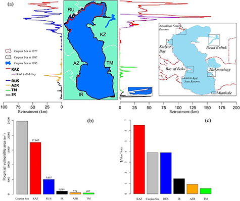
Figure 3. Spatial vulnerability of coastal areas of the Caspian Sea to SWL fluctuation: (a) coastline retreat ( ) in the west and east of the Caspian Sea and maps showing location of important gulfs in the sea, (b) potential vulnerable area (
 ) of the Caspian Sea and surrounding countries and c) vulnerability ratio (v in
 ) for the Caspian Sea and all surrounding countries (KAZ = Kazakhstan, RUS = Russia, IR = Iran, AZR = Azerbaijan, TM = Turkmenistan).
Download figure:
Standard image High-resolution image
Figure 4. Vulnerability ranking of the Northern, Middle and Southern Caspian Sea to SWL fluctuations: (a) potential vulnerable area and coasts of the Northern, Middle and Southern Caspian, (b) sea water depth, (c) linear regression between SWL and CVA of the Caspian Sea, and (d) sensitivity analysis of SWL simulation model to evaporation, total inflow and precipitation based on method of Morris (1991).
Download figure:
Standard image High-resolution imageThree ecologically important bays on the eastern coast, Dead Kultuk, Türkmenbaşy and Miankale, are highly vulnerable to SWL fluctuation (figure 3(a)). As shown by purple curve in figure 3(a), the majority of potential coastline retreatment in Kazakhstan is in Dead Kultuk and potential vulnerable areas in Iran are mainly located in the Miankale Gulf. Marginal shallow gulfs in the south of Russia, centre of Turkmenistan and south of Azerbaijan are also vulnerable to coastline retreat compared with past historical observations. For example, in Türkmenbaşy Bay, the sea retreat can be more than 25 km. In Azerbaijan, although the Bay of Baku shoreline has experienced no change during the past 80 years, the coastline retreatment in Ghizil-Agaj State Reserve is considerable. In the west of the Caspian Sea, the Kizlyar region is the most vulnerable area. Astrakhan Nature Reserve on the western shoreline is another highly vulnerable region. Around 90% of the potential vulnerable area of the sea is on the Northern Caspian coast, 10% is on Southern Caspian coast, and less than 100 km2 (0.4%) is on the Middle Caspian coast.
3.2. SWL-CVA linear regression and sensitivity analysis of SWL to change in  and
and


Based on the available images from 1977 to 2018 (33 NDWI maps) and SWL data for this period, the relationship between SWL raise in m (MSL) and CVA in km2 was calculated at different scales from the whole of the Caspian Sea to coastal regions in surrounding countries (table 1). The slope of the linear regression between SWL and CVA for the whole of the sea was  m–1 (figure 4(c)), which indicates that with a 1 m rise in SWL, about 7700 km2 of the potential vulnerable area of the Caspian Sea would be covered. Linear approximations in table 1 are restricted to a period from 1977 to 2018 (
 ) so, based on assumptions in regression models, any extrapolation of a fitted regression equation beyond the range of SWL can lead to biased estimates.
Table 1. Relationship between sea water level (SWL, m) and covered potential vulnerable area (CVA,  2) for the Caspian Sea and surrounding countries.
| Region | Equation | r2 |
|---|---|---|
| Caspian Sea |  |
0.91 |
| Northern Caspian |  |
0.90 |
| Middle Caspian |  |
0.68 |
| Southern Caspian |  |
0.56 |
| Kazakhstan |  |
0.88 |
| Russia |  |
0.42 |
| Iran |  |
0.65 |
| Azerbaijan |  |
0.75 |
| Turkmenistan |  |
0.66 |
Results of sensitivity analysis (figure 4(d)) indicate that the overall importance of evaporation (represented by  ) on the SWL simulation model output is highest followed by total inflow and precipitation respectively. In terms of
  , total inflow has the highest value followed by evaporation and precipitation that means total inflow is the variable involved in interaction with other variables and its effect is non-linear in SWL simulation model.
3.3. Equilibrium state of the Caspian Sea
We found that each 1 km3 inflow alteration changes the equilibrium SWL by about 16–18 cm, while each 10 mm variation in P-E changes the equilibrium SWL by about 6–6.5 cm. It should be noted that the highest SWL in the Caspian Sea from 1980 to 2018, the period for which the SWL-CVA relationship is developed, equals to −26 m (in 1995). However, in the 1880s,  m has been observed. Therefore, heatmaps of CVA for different parts of the sea (figure 5) were produced by extrapolating the SWL-CVA relationship for the range from −26 to −25.5. In this range, some coastal areas which were dry in 1995 will go under water and CVA can reach 27 500 km2 in figure 5(b), i.e. more than potential vulnerable area (25 000 km2).
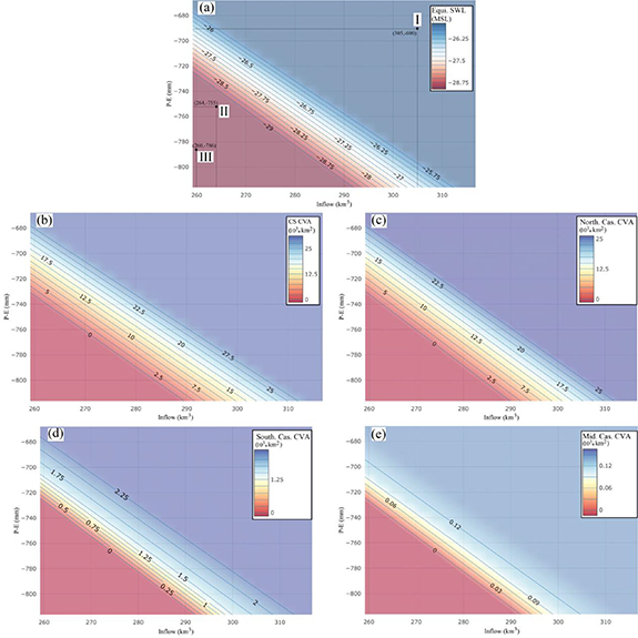
Figure 5. (a) Equilibrium sea water level (SWL in m) of the Caspian Sea (CS) based on different combinations of total inflow and net precipitation (P-E) and CVA in equilibrium state for: (b) the Caspian Sea, (c) Northern Caspian coast (North. Cas.), (d) Southern Caspian coast (South. Cas.), and (e) Middle Caspian coast (Mid. Cas.).
Download figure:
Standard image High-resolution imageThe highest SWL in the Caspian Sea observed from 1840 to present was −25.5 m, so we considered equilibrium SWL more than −25.5 as one class (blue zone: full state, figure 5(a). Available records indicate that SWL less than −29 m has not occurred in the past, so equilibrium SWLs below −29 m are also categorised into one class in figure 5(a) (red zone: worst state). In 1987, when SWL was −27.7 m, the Dead Kultuk Bay was completely desiccated, shown in figure 3(a). We show this SWL in figure 5(a) as a white zone in the heatmap, before restoration work on Dead Kultuk Bay as an important environmental icon of the Caspian Sea. Therefore, around −27.7 m is a transient SWL between warning and restoring zones of the equilibrium SWL heatmap in figure 5(a).
Using calculated equilibrium  (figure 5(a)) and
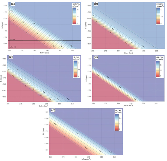
  regression model (table 1), we quantified CVA and water balance parameters (net precipitation and inflow) relation separately for surrounding countries of the sea in figure 6 As shown in this figure, Kazakhstan is the most vulnerable country by almost 18 000 km2 of potential vulnerable area. In recent years from 2010 to 2015, the average of
  mm and
  km3. Under current situation, to recover all vulnerable area of Kazakhstan (reaching the contour of 18 000 km2), the total inflow should increase from 260 to more than 300 km3 or net precipitation should increase from −786 to −680 mm. Also, contour 18 000 km2 determines other possible combination of
  and
and  for recovering all potential vulnerable area in Kazakhstan. As described before, to go beyond 18 000 km2 and reach 20 000 km2 contour, the SWL of the sea should increase from −26 m (highest observed SWL in 1995) to −25.5 m.
Figure 6. Covered potential vulnerable area (CVA in km2) in equilibrium SWL based on different combinations of total inflow and net precipitation (P-E) for (a) Kazakhstan (KAZ), (b) Russia (RUS), (c) Iran (IR), (d) Azerbaijan (AZR) and e) Turkmenistan (TM).
Download figure:
Standard image High-resolution image
4. Discussion
The results obtained in this study illustrate the spatial consequences of hydro-climatological alterations on water level in the Caspian Sea. In a novel approach, we determined separately how SWL variation can affect desiccation of marginal gulfs of the Caspian Sea. First, we determined potentially vulnerable area of the sea to SWL fluctuation and developed the regression model on SWL-CVA relation. Then we quantified the effect of changes in  ,
, and
and  on the desiccation of vulnerable areas combining water balance simulation model and CVA-SWL regression. Also, sensitivity analysis of water SWL simulation model showed that evaporation plays an important role in this model. This is crucial because significant increases in evaporation over the Caspian Sea is expected under climate change scenarios (A1b and A2) (Elguindi and Giorgi 2006).
Since the 1930s, three major trends in SWL were identified, in 1940–1977, 1977–1995 and 2000s-present (figure 2.(a)). In these periods, average  (km3) was 264, 305 and 260, and
  (mm) from CFSR was −755, −690 and −786, respectively. The trend over 1940–1977 cannot be considered as a period of natural tendency of SWL because, in this period as a consequence of dam construction, a massive water accumulation in reservoirs as well as partial evaporation and water withdrawal from reservoirs of dams on major rivers (e.g. Volga, Ural, and Kura) has occurred (Shiklomanov 1976). As markied in figure 5(a) (point I), for 1977–1995,
  combination is in blue zone of the equilibrium SWL heatmap where SWL is more than −25.5 m, while observed SWL in this period is between −29 to −26 m, i.e.
  exceeded
  and level started to increase. Also, in the periods 1940–1977 (point II) and 2008–2015 (point III), the equilibrium SWL is in red zone and lower than the observed SWL which can justify declining trend of the SWL in these periods. In other word, if mean of
  stay constant in long term, the SWL will keep changing to reach equilibrium state. In the most recent 10 years, the existing combination of
 and
and  is even worse than the period 1940–1977 and if this situation continues, it will result in lower SWL than observed in the 1970s.
In some recent environmental disasters in the region, such as Aral Sea, the water level decline is due to unsustainable use of water resources (Madani 2014). Despite warnings, lack of good quality information has affected decision making and restoration policy (Akbari et al 2019). The equilibrium state concept can be an appropriate indicator to predict the final status of water bodies under current hydro-climatological situation, because the equilibrium state is defined based on integration of P, E and  effects on SWL in the long term. Development plans in countries surrounding the Caspian Sea can also be evaluated by calculating the equilibrium state based on imposed hydro-climatological status.
Precipitation is predicted to decrease by about 10% over the Caspian Sea (Roshan et al 2012) and significant increases in evaporation is expected (Elguindi and Giorgi 2006). Climate conditions at present (point III in red zone of figure 5(a) and future (climate change scenarios) both pose a threat for the Caspian Sea. As mentioned before, each 10 mm decrease in  can reduce equilibrium SWL by about 6.5 cm. In addition, the slope of the SWL-CVA relationship is
  km2 m–1 so each 10 mm decline in
  is equivalent to about 500 km2 (
 ) of potential vulnerable area desiccation. The long-term average of
  over the Caspian Sea from the 1930s is −750 mm. Therefore, a 5% reduction in P—E (≈37.5 mm) can lead to a 24.4 cm reduction in equilibrium SWL and desiccation of 1875 km2 of potential vulnerable area. Also, a 1 km3 decline in inflow will alter the equilibrium SWL of the Caspian Sea by 16–18 cm (see section 3.3). According to the slope of the SWL-CVA relationship (table 1), this reduction in SWL is equal to desiccation of about 1400 km2 (
 ) of the potential vulnerable area of the sea. This desiccation as a result of climate change or river flow manipulation would not be limited to a specific region but would affect all over of the Caspian Sea as an ecological system.
In March 1980, in order to decelerate a continuous fall of the Caspian Sea level the Garabogazköl was dammed. In response to this human intervention, the bay had already dried up completely by November 1983. In 1992, the dam was destroyed, and this bay had been filling up with the Caspian Sea water (Kosarev et al 2009). Therefore, change in relation between area of the sea and SWL should be checked before and after 1992 because geometry around Garabogazköl has changed which affects hydrological situation of the sea and outflow from the Caspian Sea to Garabogazköl through broken dam location. This event may change water balance of the Caspian Sea significantly. In appendix A, water body maps of the Garabogazköl approve that the area of this bay has increased after 1993. To differentiate between area and SWL regression before the dam break (1977–1992) and after it (1993–2015), we defined dummy variables to check whether linear regression of the Caspian Sea is significantly affected by Garabogazköl dam break or not. The t-value of dummy variables approved that this regression for whole of the Caspian Sea is not significantly affected by the dam break phenomenon in 1992. More details on linear regressing before and after 1992 as well as t-value of dummy variables are presented in appendix B. Although dummy variable, approved that dam break phenomenon did not have statistically significant effect of area and SWL regression, dam break event is detectable by the error analysis of presented regression model in figure S4 (appendix B) (available online at https://stacks.iop.org/ERL/15/115002/mmedia). As marked in this plot, years before 1992 has the highest error compared to other points which roots in insignificant different geometry condition before 1992.
We neglected groundwater inflow in the water balance analysis, because it is estimated to be small (Zekster 1995, Arpe et al 2013, Chen et al 2017), so this can be considered a source of uncertainty. Lack of adequate in-situ measurements of e.g. major river flow and outflow to adjacent bays, particularly Garabogazköl in Turkmenistan, were other sources of uncertainty in this study. In addition, the data on SWL were taken from satellite altimetry products and observed values in tide gauges, which were produced by two different methods. Data on precipitation and evaporation from the CFSR model were validated against in-situ records, but CFSR products were source of error. Furthermore, the NDWI threshold used for identifying water bodies (greater than zero) was taken from the literature (Gao 1996, Mcfeeters 1996) and more detail on the estimation of area by different thresholds for NDWI is discussed in appendix A. For NDWI calculations, different sources of data from Landsat 2 MSS to Landsat 8 OLI, which have different spectral resolution, were utilised. Therefore, we estimated NDWI using different formulae. Quantifying and decoupling the effect of anthropogenic activities and climate change effect on the fluctuation of SWL in Caspian Sea is a potential area for further studies. In this study, we addressed the effect of change in water balance parameters on desiccation of different regions of the sea, but the question on why SWL has changed is yet unanswered.
5. Conclusions
More than 60% of the Caspian Sea shoreline is surrounded by an arid climate where consumption of water for economic development and water supply by desalination could be very attractive for developing countries. The reservoir capacity of dams in the Caspian Sea basin is more than 75% of total inflow increasing the susceptibility of the Caspian Sea to anthropogenic regulation on rivers. Considering uncertainty in climate change models in forecasting, significant decline in net precipitation is expected under different climate change scenarios. Although Kazakhstan, the most vulnerable country, has no control on river flows to the sea, coastal regions in that country will be mostly affected by potential desiccation. All surrounding countries will be affected by their gulf desiccation if SWL declines. Therefore, it is crucial for the Caspian Sea to have an inclusive governance approach that engages all surrounding governments as principal contributors to sustainable water resource management in the Caspian Sea basin as a single ecosystem.
Acknowledgments
The authors are thankful to anonymous reviewers who provided insights and expertise that greatly assisted the research.
Data availability statement
The data that support the findings of this study are available upon reasonable request from the authors.