


Abstract
Climate change is making water supply less predictable, even unreliable, in parts of the world. Urban water providers, especially in already arid areas, will need to diversify their water resources by switching to alternative sources and negotiating trading agreements to create more resilient and interdependent networks. The increasing complexity of these networks will likely require more operational electricity. The ability to document, visualize, and analyze water–energy relationships will be critical to future water planning, especially as data needed to conduct the analyses become increasingly available. We have developed a network model and decision-support tool, WESTNet, to perform these tasks. Herein, WESTNet was used to analyze a model of California's 2010 urban water network as well as the projected system for 2020 and 2030. Results for California's ten hydrologic regions show that the average number of water sources per utility and total electricity consumption for supplying water will increase in spite of decreasing per-capita water consumption. Electricity intensity (kWh m−3) will increase in arid regions of the state due to shifts to alternative water sources such as indirect potable water reuse, desalination, and water transfers. In wetter, typically less populated, regions, reduced water demand for electricity-intensive supplies will decrease the electricity intensity of the water supply mix, though total electricity consumption will increase due to urban population growth. The results of this study provide a baseline for comparing current and potential innovations to California's water system. The WESTNet tool can be applied to diverse water systems in any geographic region at a variety of scales to evaluate an array of network-dependent water–energy parameters.
Export citation and abstract BibTeX RIS
Introduction
In the coming years, many countries and regions, including 40 US states, could face water shortages [1–3]. Nonetheless, in the United States, most water customers take for granted that sufficient quantities of safe-to-drink water will flow whenever they turn on the tap. Increasing population, urbanization, more restrictive environmental requirements, decaying infrastructure, contamination, droughts, and climate change—and their compounding effects—are challenging the resiliency of existing water systems and putting those assumptions at risk.
Table 1. Contributors to California's 2010 electricity and water mixes. Water mixes are shown for the North Coast (NC) and the South Coast (SC) hydrologic regions which are representative of water-rich and water-scarce conditions, respectively. Hydrologic region boundaries are shown in figure 1.
| Contributors to electricity mix | |||
|---|---|---|---|
| Type | Electricity conversion efficency (%)a | Present in 2010 state electricity mix? | |
| Coal | 33% | ✓ | |
| Natural gas | 40%−43% | ✓ | |
| Petroleum | 30%−32% | ✓ | |
| Nuclear | 33% | ✓ | |
| Hydropower (conventional) | 90% | ✓ | |
| Hydropower (small in-stream and similar) | NA | ✓ | |
| Solar PV | 12% | ✓ | |
| Solar thermal | 21% | ✓ | |
| Wind | 26% | ✓ | |
| Geothermal | 16% | ✓ | |
| Biomass | 24%–32% | ✓ | |
| Contributors to California's urban water mix | |||
| Electricity intensity | Present in 2010 regional water mix? | ||
| Type | (kWh m−3)b | NC | NC |
| Groundwater | 0.15–0.52 | ✓ | ✓ |
| Surface water | 0.072–0.23 | ✓ | ✓ |
| State water project | 0.052–4.12 | − | ✓ |
| Central Valley project | 0.052–0.78 | − | ✓ |
| Colorado River aqueduct | 1.7 | − | ✓ |
| Local water transfers | 0.052–1.5 | ✓ | ✓ |
| Stormwater capture: non potablec | 4.1 | − | ✓ |
| Recycled water: non-potable | 0.29–1.1 | ✓ | ✓ |
| Recycled water: groundwater augmentation | 0.53–1.5 | − | ✓ |
| Desalination: brackish groundwater | 0.47–1.4 | − | ✓ |
| Desalination: ocean | 3.0–3.5 | − | − |
aConversions estimated using guidelines outlined in [20], except for biomass, which was obtained from [21]. bTypical range for California's potable water, unless specified, includes electricity for supply, conveyance, and treatment, all electrical intensities dependent on the source and quality of water; distribution electricity is excluded as it is more affected by topography. See the supplementary information for more detail and citations. cOnly one stormwater capture system was evaluated in this study, thus a range is not provided.
How have arid regions addressed pressures associated with water scarcity? Historically, these regions have followed a pattern of diversifying water supplies to meet demand and increase the flexibility and reliability of their systems. Richter et al studied water supply systems in four arid cities and identified strategies that were implemented successively to address scarcity:
- 1.Exhaust local groundwater and/or surface water supplies; build local storage (e.g. reservoirs).
- 2.Transfer water from other basins until infeasible.
- 3.Conserve water.
- 4.Develop alternative water supply, including recycled water and desalination [4].
A changing climate and population growth will risk scarcity in areas not currently considered arid. Unless better strategies are identified, these areas are likely to follow a similar diversification pattern, though we expect that regions facing water scarcity will learn from the past and consider low-cost, low-risk conservation options initially.
Alternatives needed to address water scarcity are often more expensive and energy-intensive than traditional sources [5]. If utilities and water resource managers in water-scarce regions like California seek to manage the electricity intensity (EI) of water supply, they will require analytical methods and tools as well as an accurate baseline. The goal of this research is to develop an analytical network model and adaptable decision-support tool that can be used to visualize increasingly diverse, complex, and inter-connected water networks and calculate cumulative embedded electricity in water flows. The model and tool will be used together to answer the following research questions: (1) What was the estimated baseline electricity consumption for providing water to urban areas in California's ten hydrologic regions in 2010 for 1 m3 of water, for an average person's water consumption, and for the region as a whole, given publicly available data? (2) How do these estimates change given potential changes to the regional water supply mix in 2020 and 2030, as projected by each urban water utility in 2010?
The energy consumption impacts of relying heavily on unconventional alternatives is not well understood. Studies of energy systems recognize the importance of acknowledging that energy, particularly electricity, comprises a geographically-specific mix of sources. For example, electricity produced from coal in West Virginia functions on the grid the same way as electricity produced from wind in Texas, but the effects of its production, due to both fuel source characteristics and conversion efficiency, can be very different. Though water is often seen as a single uniform commodity, the ever-increasing complexity, diversity, and spatial dependence of its sourcing will affect the electricity needed to obtain and treat sources of different quality [5, 6]. Table 1 describes sources that may compose electricity and water mixes. It shows the potential range of EIs for a particular water source, depending on site-specific conditions, and illustrates that alternatives to conventional supplies tend to have higher EIs. Studies of electricity use by water systems have been previously conducted, including some that evaluated the effects of water scarcity and diversification on energy consumption in selected cities [5–9]. Though energy use generally increased with scarcity, results were mixed and depended on the locations and alternatives evaluated. Another study evaluated the spatial dependence of energy consumption associated with water distribution [10]. Further, substantial literature reviews of such studies are included in references [11, 12].
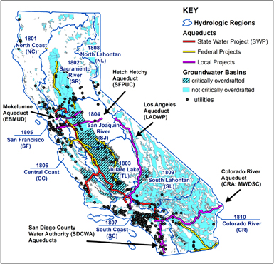
Figure 1. California's complex water infrastructure network: major federal, state, and local water transfer infrastructure. Geometries for hydrologic regions and groundwater basins from [24].
Download figure:
Standard image High-resolution imageStudies that consider the implications of large-scale water networks are less common. Researchers have published a series of spatially-explicit studies to determine where energy production is needed to meet water demand in the western United States and globally [13–15]. These studies relied on top-down aggregated estimates of water use from the US Geological Survey and do not calculate energy embedded in water consumed in a particular location. California-specific water network models exist but are designed to support economic and hydrologic analyses rather than examining interactions with energy, rely on top-down analyses that cannot easily incorporate locally-reported data, and/or require proprietary software, limiting broader application (see the literature review contained in [16] as well as in [17–19]).
California's diversifying water supply mix
Historically, California has strategically matched water supply and demand. The state gets approximately 75% of its precipitation in the higher-elevation northern and eastern regions, predominantly during California's rainy season (October to April), while around 75% of its population lives in western and southern regions. Consequently, California relies significantly on the most traditional water conveyance system: water flowing downhill—though water may flow across hundreds of miles and over mountains before reaching consumers. Mountainous regions have allowed the state to rely on snowpack to store water in the winter, when local water supplies are more readily available, before melting slowly over the spring and summer when water is needed, reducing the need for engineered storage.
California is currently grappling with myriad pressures that affect water supply and demand. Its growing urban population means overall demand increases even after dramatic conservation measures cause per-capita water consumption to fall. Climate change is expected to increase summer temperatures and change precipitation patterns, escalating irrigation demands while reducing supply by lengthening drought periods, intensifying and concentrating rainstorms, and reducing overall snowfall, challenging the snowpack-based storage system [22]. Pollution from fertilizers, industrial chemicals, and salinity caused by perpetual irrigation or seawater intrusion affects several critical aquifers. The 2014 Sustainable Groundwater Management Act (SGMA), a law intended to prevent spreading contamination or persistent overdraft, will limit groundwater pumping in water-constrained basins in the coming decades [23].
The strategies California has used historically to address these challenges are reflected in the Richter et al study [4]. Surface water and groundwater are fully, if not over, allocated (Strategy #1). Massive aqueducts owned by federal, state, and local entities span hundreds of miles throughout the state (figure 1). These aqueducts are increasingly used to facilitate water markets via short- and long-term water trading between utilities connected to them through direct transfers of unneeded water and via groundwater banking programs (Strategy #2). Conservation programs began in earnest in the 1990s and have continued (Strategy #3). Interest in more diverse water sources has increased over time, reaching a height during the recent drought (Strategy #4).
Data availability in water system modeling
Methods and tools are needed to provide a detailed analysis of increasingly diversified water supplies for all stakeholders, including water professionals, policymakers, and the general public. Understanding water systems' interconnections, the potential for these systems to diversify and innovate, and the subsequent impacts on other economic sectors, most notably the energy sector, will become increasingly important. Achieving this level of understanding will require more extensive data collection and dissemination from California's water industry. Water systems are managed locally, creating a fractured industry. Data are inconsistently reported and rarely aggregated for use in policy and planning over a wide region [25, 26]. (Data availability is further addressed in the Limitations section).
In California, groundwater aquifers are particularly poorly understood and monitored and, though the SGMA is intended to correct this [23], full implementation of the law is not expected until 2040. This and other initiatives developed in response to the drought could improve availability of water and related energy data (e.g. [27, 28]).
Ironically, some data currently available are underutilized. California's water utilities that provide more than 3000 acre-feet (3.7 million m3) or serve more than 3000 people are required to submit Urban Water Management Plans (UWMP) every five years. UWMPs provide information on water supplies and demands projected at least 20 years into the future. UWMPs have historically been difficult to analyze because they vary in quality, contain inconsistencies, and are submitted as hundreds of separate files with inconsistent formats that cannot be easily parsed. Fortunately, the 2015 reports, currently under review, required more comprehensive electronic data submission, making analysis easier in the future. Nonetheless, these UWMPs provide a useful resource in understanding the current trajectory of water development and identifying areas where innovations should be targeted to improve the resiliency and sustainability of the water network.
Methods
Given the dearth of analytical tools available to analyze complex urban water–energy connections, the plethora of untapped water data available from UWMPs, and the wealth of data that may soon become available in California, developing more comprehensive water–energy analysis methods is critical. Our research was conducted in three steps by: (1) collecting data on California's water flows and EIs (kWh m−3) for all supply, treatment, and distribution processes, using utility-specific data when publicly available; (2) compiling these data into a network model; and (3) creating the Water–Energy Sustainability Tool for Networks (WESTNet) to visualize interactions, track water flows, and calculate the total and per-capita electricity consumption, as well as cumulative EI, as the water passes through the complex water network. WESTNet is still in a beta version and is not yet ready for public release, though we anticipate this for the future. To demonstrate WESTNet, we have applied it to urban water networks in California to estimate the electricity needs of supplying water from diverse sources in 2010, 2020, and 2030. We used low, medium, and high EI estimates to bound the electricity embedded in water supply for the state and its ten hydrologic regions. This model and tool are designed to be easily updated as site-specific data become available, allowing for a bottom-up analysis of regional and statewide effects. The following sections further describe these steps.
California network data collection and electricity intensity estimation
Data for individual urban water systems from 2010 UWMPs compiled by the California Department of Water Resources (DWR) into spreadsheets were accessed for this study [29]. (The 2015 plans have been submitted but many were not reviewed and finalized in time for inclusion. We plan to analyze them in future work.)
Table S1 (found in the supporting information [SI] available at stacks.iop.org/ERL/12/114005/mmedia) contains a list of all utilities analyzed and whether they are a retail or wholesale utility. Some utilities serve both functions. Water supplies and demands for each utility were compiled for its actual 2010 operations as well as projections made by the utilities themselves in 2010 for its supplies and demands for 2020 and 2030. DWR's tables summarized water supply sources by general categories (i.e. 'surface water', 'recycled water', 'desalinated water', and 'wholesaler'). Supplies for raw (i.e. untreated water used for irrigation, groundwater recharge, and similar uses), potable, and recycled water supplies were tracked separately for each utility as demands for different quality water vary.
Electricity intensity for the federal, state, and local aqueducts as well as average estimates of treatment EIs for different water sources and ranges of distribution EI were obtained from [5, 12, 14, 30–34] as described in the SI. Tables S2–S4 summarize the EI data used for this study. For each source, a low, moderate, and high EI was identified to evaluate the range of effects possible over the analysis period using current technologies. These estimates bound the potential current and future states of electricity use for water supply in California. Water supplies that could not be assigned to a specific source category were assigned the EI for surface water sources, an assumption that likely underestimates their effect. When available, utility-specific electricity consumption data were used in lieu of default values for all three scenarios. Table S1 designates which utilities were analyzed using site-specific data.
The low scenario uses conservative estimates for default supply and treatment EI and assumes that the EIs for particular sources remain unchanged over the analysis period. Regional EIs in the low scenario change solely due to water supply diversification. In the moderate and high scenarios, the EIs for particular sources increase through the analysis period. For example, we assumed water levels in overdrafted groundwater basins (figure 1) will continue to drop through 2030 so electricity use will rise in an inversely proportional manner due to increased pumping [12]. We made exceptions for adjudicated basins, assumed to have stable groundwater depths due to court-mandated withdrawal limits. We also assumed that basins experiencing deteriorating water quality will have increasing groundwater treatment EIs. Distribution EIs were consistent over time regardless of scenario.
Network model and tool development
To build and visualize the network model, each utility and its water source mix was assigned a unique identification code as specified in table S5. Generically, nodes for a particular utility were identified using a seven-digit code beginning with the four-digit hydrologic unit code (HUC) of the region where the utility is located. In the text of this paper, the hydrologic regions are identified by an abbreviation. These regions, their HUCs, and abbreviations are: North Coast (1801; NC), Sacramento River (1802; SR), Tulare Lake (1803; TL), San Joaquin River (1804; SJ), San Francisco Bay (1805; SF); Central Coast (1806; CC); South Coast (1807; SC); North Lahontan (1808; NL); South Lahontan (1809; SL); and Colorado River (1810; CR). Regional boundaries are shown in figure 1. The last three digits of each utility's code are specific to that utility.
WESTNet uses a network-based approach for calculating the EI which is described in the SI. The model reports the EI at each individual node and for each hydrologic region and the state as a whole, based on the weighted average by demand volume for end-user nodes located in the appropriate boundary. More detailed discussion of the network model and WESTNet tool can be found in the SI.
Though the ability to track water flows and calculate embedded electricity through the complex network is a significant objective of this research, the value of visualizing the network should not be underestimated. WESTNet can create complete water network visualizations but also allows the user to designate a particular node and visualize the system upstream (nodes that provide water to the designated node) and/or downstream (nodes that receive water from the designated node). These relationships can be difficult to discern for industry professionals and regulators, much less customers, and are critically important. For example, in February 2017, Lake Oroville experienced an unprecedented series of events that lead to fears that the reservoir's emergency spillway would fail, causing flooding downstream in the short term and a significant loss of storage in the longer term. Lake Oroville is the largest reservoir in the State Water Project (SWP), a series of aqueducts, reservoirs, and pumping facilities that provide water to about 36 million people (figure 1). Using WESTNet, the authors were able to show that, though only 24 urban water agencies contract directly with the SWP, almost 200 could be affected by the potential failure as a result of nested wholesale contracts and transfers. (One SWP contractor is the Metropolitan Water District of Southern California (MWDSC) which serves 26 utilities of which 12 are wholesalers to additional utilities. The San Diego County Water Authority (SDCWA) is a wholesaler that buys water from MWDSC and, in turn, sells it to an additional 24 retail utilities.) The analysis and visualization were informative, as demonstrated when the results were included in media coverage of the event [35].
Figure 2 shows utilities served by the SWP. Figure 2(a) is organized in a linear configuration and presents a subset of the retail and wholesale utilities (blue nodes) which would have been affected by the failure of the emergency dam. A diagram shown as a web configuration is available in [35], though a few subsequent revisions are not reflected there. The map in figure 2(b) shows all utilities that could have been affected and illustrates how the model can be linked to a GIS platform for visualization.
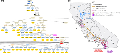
Figure 2. Two views of the network served by Lake Oroville and the State Water Project. (a) A subset of the network of utilities served by Lake Oroville. Approximately 20% of the wholesale and retail water agencies (blue nodes) that obtain a portion of their water supply from Lake Oroville and less than 8% of the full network for the state are shown here. Certain nodes have been outlined in colored and patterned circles so they can be matched when they appear in figure 3. The node outlined in dotted blue is Lake Oroville. The node outlined in dashed black is the San Francisco Bay Delta, where the outflows of the Sacramento and San Joaquin Rivers meet and connect to state aqueducts. The node outlined in solid red is the Metropolitan Water District of Southern California (MWDSC), a wholesale agency that serves many cities in Southern California. (b) This map shows the approximate service areas of all the utilities served (in pink) as well as the locations of Lake Oroville and key infrastructure along the SWP aqueduct. Two significant wholesale agencies, MWDSC and the San Diego County Water Authority (SDCWA), are outlined. Other wholesale agencies that handle SWP water are not shown unless they also serve retail customers. The numerical labels for the key infrastructure correspond to node names in figure 2(a) and replace the 'XX' in the naming convention, as in SW1807SWPXX. from [36]. Shapefiles for hydrologic regions are from [24].
Download figure:
Standard image High-resolution image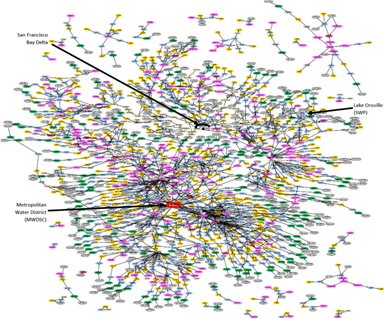
Figure 3. California's complete urban water network plotted in a web configuration. Key nodes have been outlined in hashed or colored circles so they can be matched when they appear in figure 2.
Download figure:
Standard image High-resolution image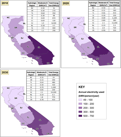
Figure 4. Actual (2010) and projected (2020 and 2030) electricity consumption for water supply, average EIs, and per-capita embedded energy for the moderate scenarios for urban water utilities in all ten of California's hydrologic regions. The moderate scenario assumes average electricity intensities for each source of water supply and that groundwater pumping requirements in overdrafted basins will increase over time, as outlined in the SI. The embedded electricity in water supply per capita for each region is indicated by regional shading.
Download figure:
Standard image High-resolution imageFigure 3 shows the state's 2010 water network plotted in a web configuration. Approximately 1500 nodes and 1800 connections are shown. This visualization highlights the interdependencies of many utilities, though it is admittedly difficult to decipher. The linear configuration of the entire system is difficult to view in a format suitable for publication due to its size. The nodes shown in a linear configuration in figure 2(a) represent less than 8% of the full state network. Both the linear and web configurations are included as svg files in the SI and are viewable at any scale in a web browser.
Results
Using WESTNet, we analyzed California's urban water network for 2010, 2020, and 2030 for the three EI scenarios described above. Figure 4 shows the total electricity consumption for water supply (GWh year−1), EI (kWh m−3), and per-capita (kWh person−1 year−1) results for each of California's ten hydrologic regions for the moderate scenario. The total water demand (million m3) evaluated in this study and the per-capita water demand for the state and each region are presented in table S6. Numerical results for regional average EIs, per-capita embedded electricity, and total embedded electricity consumption for all regions, scenarios, and years can be found in table S7.
Between 2010 and 2030, the average EI for California increases by 11%–16% under all three scenarios, though the average EIs for the NC, TL, and SF regions vary by less than 5% across the analysis period. The EI results for the SL and CR regions decrease between 2010 and 2030 for all scenarios; for the low scenario, the 2030 results are 88% and 68% of the 2010 values, respectively. The 2030 EI results for the SJ region decrease in the low scenario but are similar to 2010 results in the other scenarios. The SR, CC, and SC results increase by 6%, 17%, and 16% for the low scenario and 9%, 20% and 20% for the high scenario, respectively, between 2010 and 2030. Other trends in the EIs can be observed in table S7.
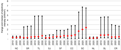
Figure 5. Statistical summary of results for utilities within each region displaying the range of results across scenario: the minimum EI for the low scenario and the maximum EI for the high scenario shown on the black line and the median EI for the moderate scenario indicated by a red diamond.
Download figure:
Standard image High-resolution image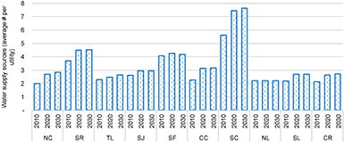
Figure 6. Average number of water sources used by each utility in the region for 2010, 2020, and 2030, as estimated based on utility reports.
Download figure:
Standard image High-resolution image
The changes in EI for future years result from source shifting. Regions with decreasing EI are generally reducing imports and/or groundwater pumping in critical basins while relying more on non-potable recycled or raw water (in agricultural areas) and surface water transfers. Using low assumptions, these can reduce electricity consumption. Regions with increasing EI generally are planning to utilize additional advanced treated recycled water, desalination, imports, or other high electricity-consuming alternatives.
Delivering water to the customers of the almost 370 water utilities that serve urban retail customers in California used approximately 9200 GWh in 2010 under low assumptions and up to 12 000 GWh with high assumptions. Delivering sufficient water to meet customer demand in 2020 will use 15 000 (12 000–17 000) GWh year−1. By 2030, these values increase to 14 000 GWh, 17 000, and 20 000 GWh for increasing EI scenarios. In 2001, urban water supply and treatment comprised 3% of electricity use [37]. The electricity required for urban water provision for the high scenario in 2030 (almost 20 000 GWh) would have been 8% of California's 2001 electricity consumption. This represents the electricity consumed by the water suppliers throughout the network and ignores any electricity generated from hydropower as part of the system. The results demonstrate the potential value to investments in more efficient use and provision of water, especially in a state concerned about rising energy costs and managing greenhouse gas emissions.
Per-capita water use is highly variable in magnitude in California's hydrologic regions, ranging in 2010 from approximately 0.57 m3 person−1 day−1 (150 gpcd) in the CC and SF Regions to 1.4 m3 person−1 day−1 (370 gpcd) in the hot, dry CR region [38]. Outdoor water use is a major contributor, comprising 50% of residential water use in the state on average. The size of yards, percentage of turf coverage, precipitation, and evapotranspiration all vary regionally. Water requirements for lawns in inland California are up to 2.5 times higher than in coastal California [39].
Nonetheless, per-capita water use is consistently decreasing throughout California. The 2009 Water Conservation Act required urban utilities to reduce per-capita water consumption by 20% by 2020 relative to a baseline that roughly corresponds to 2005 consumption rates [40]. We evaluated the embedded electricity contained in one person's average annual water consumption in all ten regions. Moderate results are shown in figure 4. For 2020, we assumed all utilities meet their 2020 conservation goals. (This may overestimate 2020 consumption because more extreme mandates requiring 25% reductions were enacted in 2015 in response to severe drought. The extent to which water consumption rates will rebound to pre-drought conditions is unclear.) No current policy requires continued reductions after 2020, but state leaders, including the governor, have stated that for California 'conservation must remain a way of life' [41]. We conservatively assumed that an additional 10% reduction would be achieved by 2030. Per-capita water use data are located in table S6.
For moderate assumptions, the 2010 results ranged from around 65 kWh person−1 year−1 in the wettest parts of the state (NC and NL) and up to 750 kWh person−1 year−1 in the SL region. The SC region, the largest consumer of water by total volume, consumes almost 500 kWh person−1 year−1. All regions show reduced per-capita electricity consumption for water in 2020, except the CC region which would remain unchanged as the increasing EI of water supply outweighs the lower per-capita water use. By 2030, all regions have lower per-capita embedded electricity compared to 2020, with the SC region dropping to 440 kWh person−1 year−1. Table S7 contains the average electricity use for water supply per capita in each region for all scenarios.
Even regional estimates for the electricity consumption of water supply, though helpful for planning purposes, fail to capture the variability of water mixes in California. Figure 5 shows the median EI in the moderate scenario for all retail utilities in each region and the range between the minimum (for low scenario) and maximum (for high scenario) values. In some regions, e.g. NC and NL, the variability between utilities is low. These regions have relatively few retail utilities (13 and 5, respectively) and abundant water resources, making significant water supply diversification unnecessary. Some regions have few utilities and still display significant variability. The CR, SL, and SJ regions all have fewer than 20 utilities. The remaining regions are represented by between 26 and 164 utilities. Utility locations are shown in figure 1. The numerical ranges for utilities in each region for all scenarios are in table S8.
Figure 6 shows the average number of water sources utilized or projected for use in each region for each year analyzed. Because water source reporting by utilities is not standardized, water sources from the same physical source (e.g. river or aquifer) may be counted twice if they were obtained through separate contractual agreements while, in other cases, wholesale contracts count as one source when multiple physical sources are used. Consequently, these results are estimates. They indicate a general increase in water supply alternatives, an effect more pronounced between 2010 and 2020 and also in more arid and/or populated regions.
Limitations of the analysis
The analysis presented herein has limitations. The UWMP data are imperfect for the detailed water accounting desired. The general water supply categories assigned by DWR (i.e. 'surface water', 'recycled water', and 'wholesaler') were not sufficiently detailed to assign all EIs. Given that the UWMPs do not use a standard, easily-parsed data format, it was unrealistic to rigorously review each individual file to supplement the data tables provided by DWR, except in specific cases. We assigned a general water source node when specific information about the source (e.g. the groundwater basin or reservoir) was unavailable or when volumes for multiple sources were aggregated in the UWMP. As a result, the network is likely more interconnected than currently shown. Examples of general source designators include: groundwater (GW), local surface water (SW), imported or wholesaler water (IMP), and wastewater treatment plant (WWT) providing recycled water (REC). Table S5 provides a complete list. Local surface water sources were generally unidentified. Additional assumptions and references used to identify specific water sources are further described in the SI.
Volumetric estimates are uncertain due to inconsistent reporting periods and water loss accounting. Each utility can pick the reporting period covered by their data to be the calendar or fiscal year and therefore volumes reported for transfers between two utilities can be inconsistent in their respective UWMPs. Because data are reported annually, rather than monthly, these inconsistencies could not be corrected and contribute significantly to the uncertainty of the results. Water losses from utility distribution systems, when estimated by the utility, are included in the utility's reported demand. The method of estimating losses was not consistently reported and the authors noted that some utilities reported surprisingly low values. Water losses associated with supply systems, including the large interbasin conveyance systems, were not considered in the analysis.
The analysis of electricity consumption predominantly uses default, general assumptions about the EI associated with water sources, treatment processes, and, on a regional basis, distribution. Groundwater supply EIs are particularly uncertain. The model does not account for the possibly substantial variability in influent quality and operational design and efficiency or other site-specific factors for each utility in a rigorous way. This is a limitation of the current analysis and not the model itself. If utility-specific data were available, this model could be easily updated accordingly.
Further, this analysis evaluated the average EI of a water supply mix assuming all sources are used equally to meet demand, given a particular quality (potable, non-potable, raw). Because it does not assign a 'loading order', or priority of use among water sources, it may not reflect the actual EI for a particular utility. In practice, a utility may choose to forgo a more electricity-intensive source in favor of a less intensive source, or vice versa. A more electricity-intensive source may be preferred, for example, to avoid financial penalties if water remains unclaimed when 'take-or-pay' contracts exist. Also, for certain sources, especially water imported by local, state, and federal agencies, multiple water utilities are served in a priority order determined by complicated water rights. When water is conserved by a water utility with a more senior water right, it may be purchased by another utility connected to the same system. The EI associated with this new water use may be lower or higher than the current use. These relationships are not captured in the model and contribute to its uncertainty.
The analysis also does not represent the current water systems as it does not reflect any additional planning, diversification, or conservation that results from the recent historic drought. We expect that using the data from 2015 UWMPs, currently under review by the DWR, would increase the EI of the water due to increased use of highly-treated recycled water, desalinated water, and other alternative sources. However, total electricity and per-capita consumption for water provision may be lower in some cases due to conservation. Regardless, the analysis of the 2010 system, not yet affected by severe concerns about system reliability, provides a baseline for benchmarking current and future innovation within and beyond California.
Finally, large-scale water–energy analyses are often limited by data availability [42, 43]. Water utilities are hesitant to release detailed data on their systems, citing valid concerns about security and privacy. Data availability has been limited and standardization poses a continual problem for the water industry [26]. However, if data collection and sharing within the industry increase, as legislative action in California encourages, the uses of this tool will expand and the accuracy of its results will improve. Even the latest submission of 2015 UWMPs in California has made the types of data which had to be laboriously mined for this analysis more readily accessible and comparable. This alone will do much to improve our understanding of the interconnected urban water system in California and its effects on statewide electricity consumption.
Additional analytical challenges, including specific efforts made to identify water sources and avoid double-counting of water transfers, are outlined in the SI. Though there are several sources of uncertainty in this model, many of which may be corrected with more complete and consistent data reporting in the future, as a first order estimate of the benefits of water savings, the values determined here should suffice.
Discussion
To study and visualize the interconnections of a diversified water network, we developed an analytical model of California's system and a decision-support tool, WESTNet, that can organize network connections from the bottom up, calculate cumulative embedded electricity, and evaluate EI throughout an inter-connected network for water supply sources identified for all urban water supply utilities. Preliminary release of WESTNet's visualization of the SWP supply network has proven to be effective for engaging and educating stakeholders about California's complex water system.
Any tool developed for system analysis has to balance the need for complexity, adaptability, usability, and flexibility. Other existing tools are designed to address complex economic and hydrologic interactions in California's water system data [e.g. 16, 18]. In contrast, WESTNet was designed to visualize and evaluate the energy effects of technological innovations on networks, though it can be applied more broadly. It intentionally prioritizes adaptability and flexibility over other needs. It can be adapted using publicly-available and/or locally-reported water–energy data. By design, WESTNet's framework is flexible. Users can analyze systems of varying size, scale, and complexity to address a wide variety of research questions. In this study, we have used WESTNet to calculate embedded electricity in California's water supply. Table 2 summarizes other ways the model can be used to address an array of research and/or policy questions. As previously mentioned, WESTNet is in beta version. In future work, we hope to improve the usability of the tool so it can be useful for a broader audience.
Table 2. Potential applications for the WESTNet decision-support tool.
| Tool is flexible with regard to: | How it is used for this study | Examples of additional possible uses for WESTNet |
|---|---|---|
| Scale | State | Examine a country, region, city, or individual facility, including a combination of centralized and decentralized systems |
| System type | Urban water | Analyze non-urban water, wastewater, and/or reuse networks |
| Geography | California's urban water systems | Evaluate other countries, states, regions |
| Complexity | Included nodes for major pumping facilities, distribution networks, and a single end user for each utility; treatment electricity use is applied at the last supply node prior to distribution | Apply to supply from individual wells or intake points; different treatment plant or for processes within the plant; alternative water saving measures; or individual end-use sectors to evaluate fit-for-purpose water |
| Time horizon | Five-year intervals between 2010 and 2030 | Study any time interval using multiple scenarios: hourly, daily, seasonally, annually and as far into the future as desired |
| Data source | UWMP-reported data from 2010, primarily | Use more recently-reported or site-specific data or to evaluate alternative sources |
| Metrics | Embedded electricity | Quantify embedded total primary energy, cumulative water losses, salinity or other concentrations, production costs |
The results of this study can be used to estimate the electricity savings associated with conservation measures implemented throughout the state and to better target high water uses in high EI areas. In California, interconnected water flows, diversification patterns, and subsequent electricity requirements from this study—or updated analyses using more precise, site-specific data—can be useful for policy analysis at a state or regional level, for instance, by incorporating projections into plans developed for Integrated Water Regional Management Plans or Groundwater Sustainability Plans. The results can also be informative to utilities interested in comparing the electricity intensity of water supply alternatives to their existing sources or to the regional benchmark. The tool may also enhance public understanding of the source of their water, its embedded electricity, and the management of California's water system as a whole.
Conclusions
These results indicate that assuming a single EI value for delivered water, especially in arid and/or drought-prone regions like California, can be substantially inaccurate if applied broadly. Even within neighboring utilities, significant variability exists. Numerous water and energy studies make broad generalizations about water sources, assuming them to be fairly uniform. This study explicitly demonstrates the inaccuracy of that assumption. Understanding the geographic- and source-related dependencies for electricity consumption in water systems requires more detailed analysis. This paper presents a method for evaluating the electricity implications of diversifying water supplies in any setting at any scale. This paper introduces a flexible, adaptable tool for analyzing water networks. Future work will capitalize on the flexibility of WESTNet by examining potential changes to electricity use by the water network due to outside pressures (population growth, drought, and climate change) or technological innovation as well as examining other potential effects, including water losses and embedded greenhouse gases. The WESTNet tool is still in beta version, thus it is currently not available for public use but we intend to release it in the future.
Acknowledgments
The authors thank Vince Tidwell of Sandia National Laboratory for providing data on electricity use by water systems that motivated this study. We thank Paige Miller, Spencer Vanderheyden, and Greg Hori for their contributions to this research. Funding for this research was provided by the National Science Foundation-funded Reinventing the Nation's Urban Water Infrastructure (ReNUWIt) Engineering Research Center (http://renuwit.org; NSF Grant Number CBET-0853512). Any opinions, findings, and conclusions or recommendations expressed in this material are those of the authors and do not necessarily reflect the views of the NSF.
ORCID iDS
Jennifer Stokes-Draut https://orcid.org/0000-0003-0240-1361