Article

Mapping European Spruce Bark Beetle Infestation at Its Early Phase Using Gyrocopter-Mounted Hyperspectral Data and Field Measurements

by
Florian M. Hellwig
1,
Martyna A. Stelmaszczuk-Górska
1,
Clémence Dubois
1,*,
Marco Wolsza
1,
Sina C. Truckenbrodt
1,2,
Herbert Sagichewski
3,
Sergej Chmara
3,
Lutz Bannehr
4,
Angela Lausch
5,6 and
Christiane Schmullius
1
1
Department for Earth Observation, Friedrich-Schiller-University Jena, Löbdergraben 32, D-07743 Jena, Germany
2
German Aerospace Center, Citizen Science Department, Institute of Data Science, Mälzerstr. 3, D-07743 Jena, Germany
3
Forestal Research and Competency Center Gotha, Department of Digital Forest Information System, ThüringenForst, Jägerstr. 1, D-99867 Gotha, Germany
4
Institute for Geoinformation and Surveying, Anhalt University of Applied Sciences, Bauhaustr. 8, D-06846 Dessau-Roßlau, Germany
5
Helmholtz Centre for Environmental Research—UFZ, Department Computational Landscape Ecology, Permoserstr. 15, D-04318 Leipzig, Germany
6
Geography Department, Humboldt University Berlin, Unter den Linden 6, D-10099 Berlin, Germany
*
Author to whom correspondence should be addressed.
Remote Sens. 2021, 13(22), 4659; https://doi.org/10.3390/rs13224659
Submission received: 30 September 2021 / Revised: 10 November 2021 / Accepted: 13 November 2021 / Published: 18 November 2021
(This article belongs to the Special Issue Imaging Spectroscopy of Forest Ecosystems)

Abstract

:
The prolonged drought of recent years combined with the steadily increasing bark beetle infestation (Ips typographus) is causing enormous damage in Germany’s spruce forests. This preliminary study investigates whether early spruce infestation by the bark beetle (green attack) can be detected using indices based on airborne spatial high-resolution (0.3 m) hyperspectral data and field spectrometer measurements. In particular, a new hyperspectral index based on airborne data has been defined and compared with other common indices for bark beetle detection. It shows a very high overall accuracy (OAA = 98.84%) when validated with field data. Field measurements and a long-term validation in a second study area serve the validation of the robustness and transferability of the index to other areas. In comparison with commonly used indices, the defined index has the ability to detect a larger proportion of infested spruces in the green attack phase (60% against 20% for commonly used indices). This index confirms the high potential of the red-edge domain to distinguish infested spruces at an early stage. Overall, our index has great potential for forest preservation strategies aimed at the detection of infested spruces in order to mitigate the outbreaks.

1. Introduction

1.1. Motivation

Bark beetle infestation is one of the main plagues of spruce forests. In Germany, recent years were characterized by long lasting drought and high temperatures, which facilitated the spreading of bark beetles. Spruce is the dominant tree species in the Free State of Thuringia, Germany, covering almost 40% of the forest area. In 2020, the high dynamics of the development of the spruce bark beetle has continued, even though precipitations increased between 2018 and 2020 (the yearly precipitation deficit compared to the reference period 1961–1990 decreased from 27% to 6%) [1]. The amount of damaged wood has increased in 2020 to 2.9 million cubic meters, and is around 25% above the total volume of 2019 (2.3 million m3) [2]. The duration of the bark beetle attacks and their impact on trees is characterized by several phases [3,4,5,6,7]. Three main phases named after the corresponding coloration of the tree are distinguished: the “green attack” corresponds to the first stage of the attack, whereby the tree is already infested but the needles remain visually intact. A subsequent discoloration of the needles can be observed (“red attack”) in the second stage [4,7], until the needles fall completely off the tree (third stage, “grey attack”). The green attack usually lasts several weeks, depending on the region. In the Free State of Thuringia, the green attack has been observed by ThüringenForst to take 6–10 weeks. The removal of infested trees should happen before the emergence of the next bark beetle generation. The early detection of the infested trees during the green attack phase is therefore the basis for a sustainable reduction in the damaged timber volumes caused by the spruce bark beetles. The infestation of spruces is accompanied by changed sap flows and nutrient content of the trees [4,5,6] that have an influence on their spectral characteristics [3,7]. So far, infested trees have been identified too late to be removed in a timely manner [8]. Therefore, new methods are needed for detecting infested trees during the earlier phase of the infestation, i.e., the green attack. Especially, small scale spectral variations can be expected in the tree crown as bark beetle attack the nutrient supply of the trees during the green attack. The approach presented here aims to analyze the small spectral variations in the tree crown using hyperspectral airborne data for detecting bark beetle green attack.

1.2. State-of-the-Art

Forest protection includes the diagnosis and monitoring of forest damages caused by pests. Great attention is drawn to the bark beetles early detection, as it is foreseen that the damages induced by those insects will increase as a consequence of climate change [9]. In Europe, timber damages on spruce caused by insect infestations are most of all induced by the European spruce bark beetle (Ips typographus) [10]. Bark beetles mainly attack trees that are weakened, e.g., through environmental stress [11,12]. So far, no methods exist with which these newly infested trees can be timely identified in the green attack phase.
Currently, the identification of the infested trees is carried out by visual examination of the individual trees [13,14] or monitoring techniques, such as pheromone beetle traps [15] or trap trees [16]. However, due to the increasing size of damaged areas, ground-based monitoring methods cause a lag of sufficiency. Therefore, there is a great interest in the development of timely and cost-effective monitoring approaches using remote sensing (RS) methods, from close- (e.g., unmanned aerial vehicles (UAV)) to far-range (e.g., satellites), in order to reduce the terrestrial control efforts in the forest management.
Up to now, RS techniques have been used successfully for mapping the later stages of the spruce bark beetle infestation, i.e., “red attack” and “gray attack”, which correspond to phases after the bark beetles have left the host tree and caused its dieback [17].
RS sensors can measure changes in forest traits, including (i) biophysical and biochemical, (ii) functional, (iii) structural and geometrical characteristics of vegetation through the use of hyperspectral and thermal infrared (TIR) sensors [18]. Several approaches observe variations in the composition and proportion of photosynthetically-active pigments, such as chlorophyll A and B, xanthophyll and vegetation greenness [19], water content [20] and tree structure [21]. Suitable spectral characteristics and indicators for the detection of infested trees were found in the chlorophyll absorption spectral range from 450 to 890 nm [22], and in particular the red-edge range from 680 to 750 nm [23], as well as in the water absorption spectral range short wavelength infrared (SWIR) region from 1400 to 1800 nm [23,24]. Especially, hyperspectral data are recommended to be applied for the detection of changes in foliar biochemical concentrations [23,25,26,27]. Thermal infrared data have also proven reliable for mapping spruce bark beetle infestation at the green attack phase, as infested trees show higher emissivity than healthy trees [28,29]. Moreover, changes in forest structure corresponding to these phases can be mapped using the close-range, air- and spaceborne RS techniques [14,17,20,21,30,31,32,33,34,35].
So far, the most accurate methods for mapping bark beetle infestation based on multispectral and hyperspectral data still show less than 70% overall accuracy [22,23]. The spatial, spectral and temporal resolution of the data is hereby a crucial factor for accurate identification of bark beetle outbreaks [22,36].
Recent approaches show that attacked trees have spectral characteristics corresponding to stress already before infestation and that those differences remain during the attack [37]. As bark beetle preferably infest already weakened trees, it cannot be excluded that the observable difference in spectral characteristics between healthy and attacked trees already exist before the infestation [6]. Therefore, it can be difficult to distinguish the particular changes occurring in the spectral characteristics during the green attack phase from the one already existing before infestation, which is why observations over the whole vegetation season are recommended [37]. While such observations are feasible with satellite data, comparable surveys are more difficult to implement for UAVs or airborne vehicles, due to the required acquisition planning. However, few companies already provide early infestation software, based on multispectral and UAV data [8]. This software often generates over classification of infested trees. In contrast to this, investigations of green attack phases using satellite data often show discrepancies that are related to the mixed information due to the large pixel size [7,37,38].
Huo et al. [37] provide an exhaustive overview of existing RS methods for the detection of green attacks, including information about the considered temporal and spatial resolution as well as relevant bands for the detection. Only few approaches have investigated hyperspectral data [10,22]. One approach focuses principally on the calculation of several vegetation stress indices using a shorter wavelength in the visible green and red domain, while the other approach additionally considers red-edge and SWIR bands for feature selection in a support vector machine. With both approaches, the detection of the green attack phase was not possible, probably due to the resolution of the airborne data, which was larger at 4 m and 5 m, respectively.
Näsi et al. [39] developed an approach for the classification of single trees based on UAV acquired hyperspectral and multispectral data. Besides the detection of individual trees based on the UAV acquisitions and additional airborne laser scanning data, the authors defined several indices based on red-edge bands that proved to be helpful for the identification of infested trees.

1.3. Scope of This Study

In this preliminary study, we present an approach for detecting the green attack phase using high resolution airborne hyperspectral data acquired from a gyrocopter. Parallel field spectrometer acquisitions serve as reference for the analysis of the data.
In particular, the following research questions are addressed:
  • Is it possible to record early spruce infestation with a high accuracy of estimation using high resolution hyperspectral RS data?
  • Can particular hyperspectral indices be defined that detect and record early infestation phases, and can those be transferred on other study sites?
  • Is it possible to combine field spectrometer measurements and airborne hyperspectral measurements for the detection of early infestation?
The novelty of this study is in particular the combined analysis of hyperspectral data with field spectrometer measurements as well as the definition of new spectral indices in the red-edge domain of the electromagnetic spectrum for the detection of the green attack phase. In addition, the index with the highest accuracy with regard to green attack detection is validated at another study site.
The goal of this preliminary study is to lay the path for the creation of a systematic and integrated approach for early detection of bark beetle pest and its monitoring, considering RS data at different times and levels of acquisition with sufficient spatial and temporal accuracy.
This paper is constructed as follows: After providing an overview of the study area and the different acquisition systems Section 2 presents the implemented methodology for our approach. The obtained results for green attack detection based on field and airborne hyperspectral data are presented and validated in Section 3, and discussed in Section 4. Section 5 gives a conclusion and sketches possible further development and synergies.

2. Materials and Methods
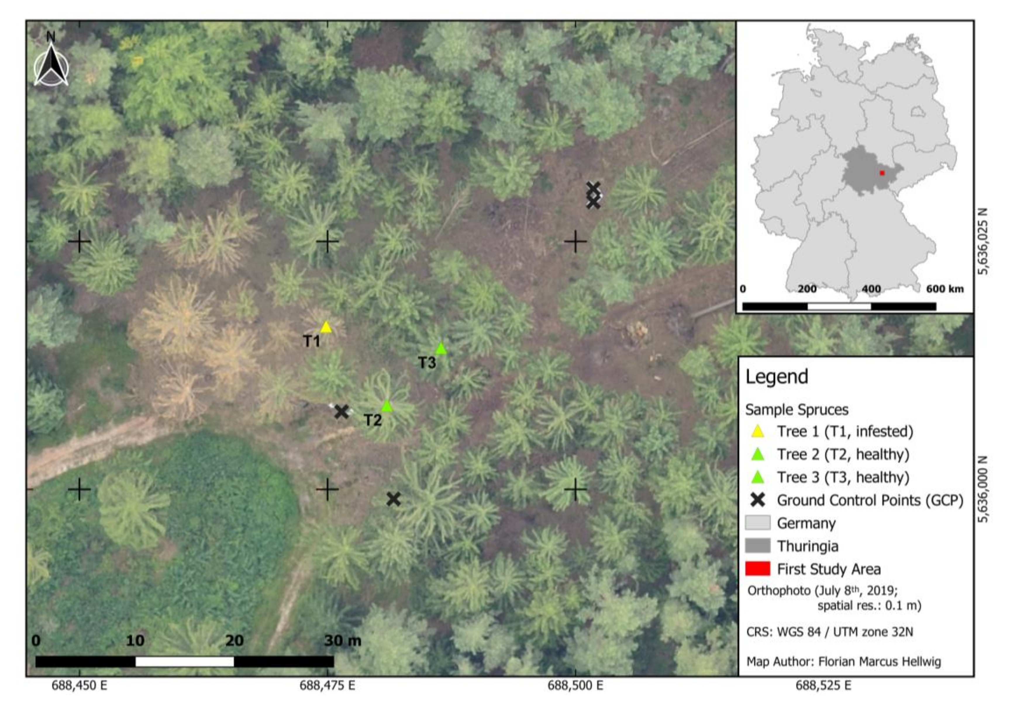
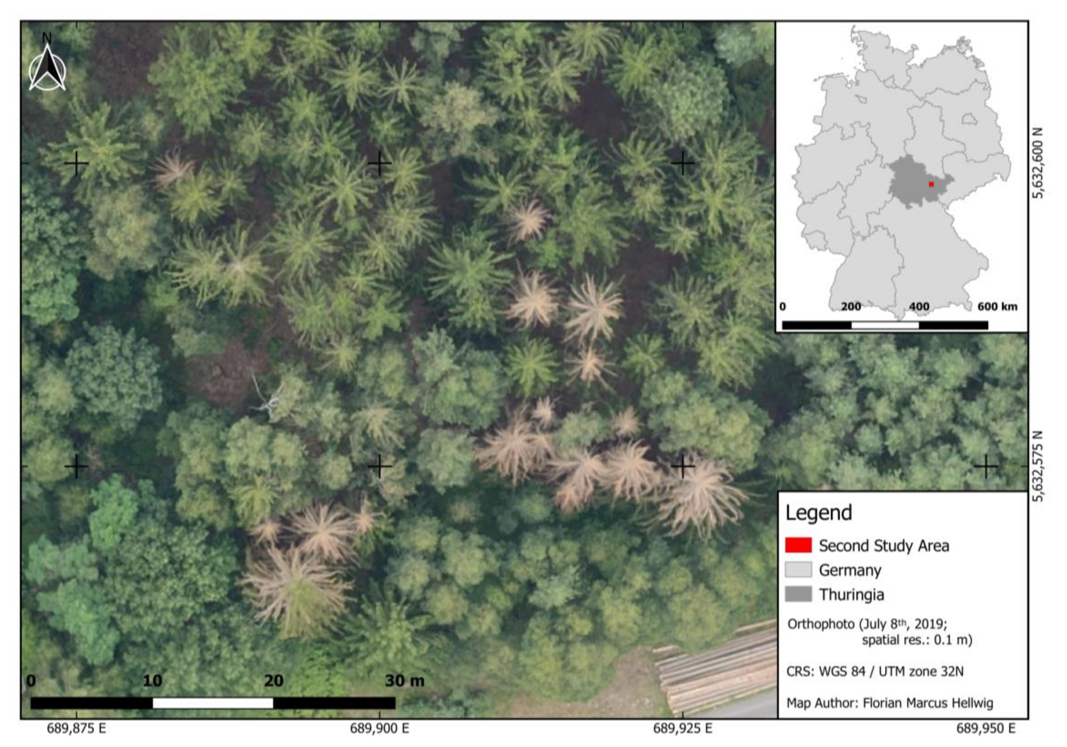
This section describes the study areas, data collection and types of data. In addition, the data preprocessing and the defined indices are explained. Finally, the classification approach for green attack detection, including validation, is presented.

2.1. Study Area

In this work, we considered two study areas, the first one for the implementation of our methodology and the second one for testing its transferability and evaluating its robustness.
The first study area (50°50′42″N, 11°40′39″E) is situated in the Free State of Thuringia (Germany), near the city of Jena (see Figure 1). The area covers approximately 4000 m2 of a forest situated in the catchment of the Roda river. The area of interest is dominated by deciduous and spruce trees.
The study area is located at 260 m above sea level and is covered by sparse, small shrubs (about 20 cm high), but no dead vegetation. The spruce trees, labeled as T1, T2 and T3, were investigated in more detail with field measurements. The spruces in the study area are about 30–40 m high (T1 ≈ 32 m, T2 ≈ 38 m, T3 ≈ 35 m) and approximately 70–100 years old. The crown diameter is about 3–8 m with an average of 5 m (T1 ≈ 4 m, T2 ≈ 7 m, T3 ≈ 5 m). More details on the collection of the samples from these trees and their labeling are provided in Section 2.2.1.
The second study area (50°48′50″N, 11°41′45″E) is about 4 km south of the first one and covers approximately 3500 m2 (see Figure 2). As in the first study area, deciduous and spruce trees are the dominating species. The study area is located at about 340 m above sea level and the spruces there are much younger (about 50–70 years) than those in the first study area. Consequently, the tree height (20–30 m) and the crown diameter (2–7 m, average ≈ 4 m) are also lower.

2.2. Data Acquisition and Instrumentation

The study areas were selected together with foresters and observed within two days in early July 2019 at different infestation stages, by a combination of hyperspectral sensors—one operated on the ground and the other in the air. On 8 July 2019, a flight campaign using a hyperspectral HySpex camera and a thermal camera mounted onboard a gyrocopter took place (see specifications in Section 2.2.2). Two days later, on 10 July, a field campaign was conducted in the first study area with a field spectrometer (for more details see Section 2.2.1). The field campaign was aimed at both mapping the positions of the investigated trees in the green attack phase, in order to better recognize and analyze them in the airborne data, as well as the acquisition of needle samples from those trees in order to analyze their spectral reflectance at different tree heights and age stages. The spectral reflectances measured in the field on three trees (T1, T2, T3) served as reference for the later comparison with spectra of the airborne hyperspectral data. The acquisition of spectra from needle samples of the trees was facilitated by their logging on the same day (10 July), allowing the sampling on trees laying on the floor. The logging of the trees only happened in study area 1. To enable a comparison with the second study area and increase the sample size, foresters shot down a few branches of another tree (T4) in study area 2. The exact position of T4 is unknown, since no global navigation satellite system (GNSS) measurement has been performed in the second study area. A fifth tree (T5), situated in study area 1, had already fallen, so its exact position was also unknown.
The acquisition of both airborne and field hyperspectral data therefore happened almost simultaneously, and facilitate the analysis of the green attack at different spatial scales.

2.2.1. Field Measurements
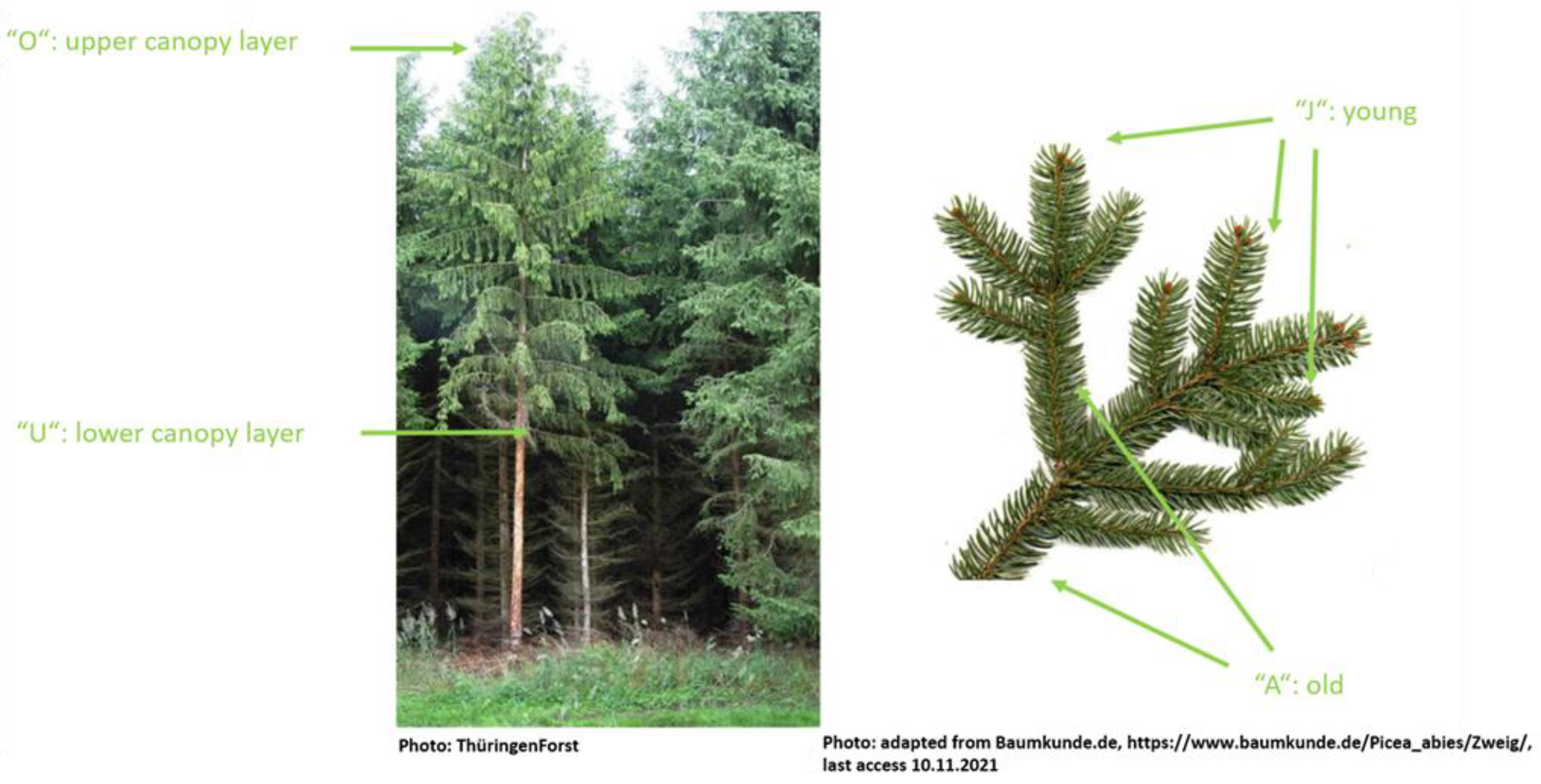
Sampling Strategies

Due to the relatively small area of interest in this preliminary study and even smaller number of trees in the green attack phase at the time of the flight campaign, five trees were selected for spectral analysis of their needles, four of which were situated in the first study area and one in the second study area (see Table 1). From each tree, four needle samples were taken, corresponding to their position in the tree and their age. Both parameters have an important impact on the spectral signature of the needles. Thus, two needle samples were acquired on the top of the tree (“O”; from German “oben”; see Figure 3) and two at the bottom of the needle canopy, closest to the ground (“U”; from German “unten”). For each canopy level, we considered each time older needle samples (“A”; from German “alt”) and young needles (“J”; from German “jung”). From the five considered trees, two were infested and in the green attack phase (T1 and T4), one already had a discolored tree crown (T5) and two trees were still healthy and not infested (T2, T3; see Table 1).
The acquisition of four different needle samples per tree is justified, since the samples may show very different spectral properties, as the upper and lower canopy is exposed differently to the sun. Moreover, older and younger needles are characterized by different pigmentation and spectral properties. In our case, additional reasons exist: first, the bark beetle infestation impacts at first the lower parts of the tree before it spreads towards the top of the crown. Second, as we want to compare the field data with RS data, it is important to consider what is visible in the RS data, which is mostly the top of the canopy and possibly some younger needles in the lower canopy layer.
In total, 20 needle samples were investigated (four positions for five trees).

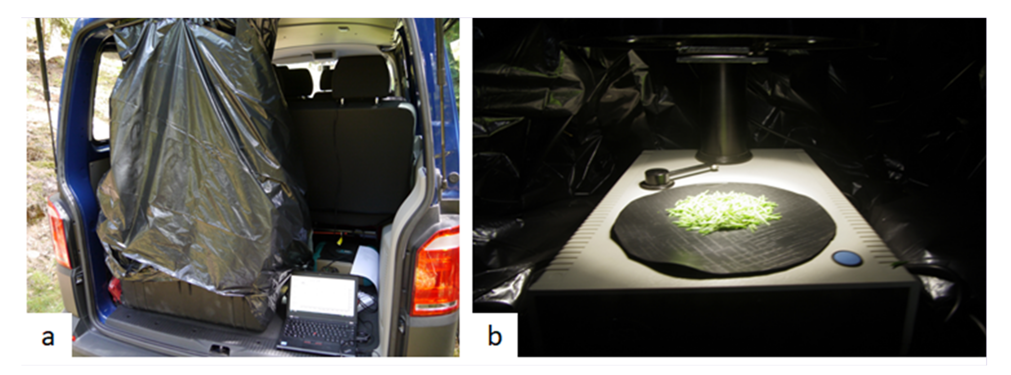
Field Spectra Acquisition

Aiming at the detection of spectral bands that are suited for a differentiation of needles of infested and healthy spruce trees based on their spectral properties, theoretical spectra should be defined under laboratory conditions. Therefore, a mobile lab was set-up in a car, allowing for a spectral sampling without external disturbance factors immediately after the harvest of the samples (see Figure 4a). The mobile lab comprised a FieldSpec 3 spectrometer (FS3; Analytical Spectral Devices Inc., Boulder, CO, USA) combined with a sample turntable (Analytical Spectral Devices Inc., Boulder, CO, USA), which was placed in a dark field cabin built of black foil that was impermeable to sunlight (see Figure 4b).
The FS 3 provides spectral data in the wavelength (λ) range from 350 to 2500 nm. The full-width-half-maximum spectral resolution was about 3 nm and 10 nm in the visible near-infrared range (λ = 350–1000 nm) and the SWIR range (λ = 1001–2500 nm), with a sampling interval of 1.4 nm and 2 nm, respectively [40]. The probe end of the 2 m long FS3 fiber cable with a 25° field-of-view [40] was fixed in the sample turntable at a nadir angle of 35°. The perpendicular distance between the fiber cable probe end and the surface of the rotatable Turntable disk was 0.11 m. At the same height, above the measurement spot on the turntable disk, a downward radiating halogen lamp (Reflekto EXT/C/A/FG; Ushio) was installed, enabling the illumination of the sample at a color temperature of 3000 K. The turntable disk was covered by a circular pool liner with a respective mean and maximum reflectance factor of 0% and 2%, in the wavelength range that the investigation will focus on (λ = 400–1000 nm).
For the acquisition of target spectra with the FS3, 5 g of the respective needle sample was randomly distributed on the circular pool liner. Digital numbers(DN) measurements were carried out in accordance with the instructions of the manufacturer [40]. In order to get rid of possible bidirectional reflectance distribution function (BRDF) effects, the rotation of the turntable disk was activated, and ten measurements were recorded and averaged for each needle sample in order to get a robust estimation of the spectral properties of the sample. A measurement of the Spectralon reference panel (SRT-99-050; Labsphere) was performed before and after each sample, in order to conduct necessary corrections during post-processing (see Section 2.3.2).

GNSS Measurements

GNSS positions of ground control points (GCPs) and trees located in the first study area were acquired with a Stonex S9III GNSS receiver. With the help of the GCPs, the orthophotos acquired with the gyrocopter were georeferenced. The GNSS positions of the trees were used to identify them in the airborne data (see Figure 1). The usual GNSS precision of a few centimeters could not be achieved, due to the measurement below the tree canopy being approximately 2 m. Nevertheless, this precision was sufficient to determine the position of the sample spruces (T1–T3).

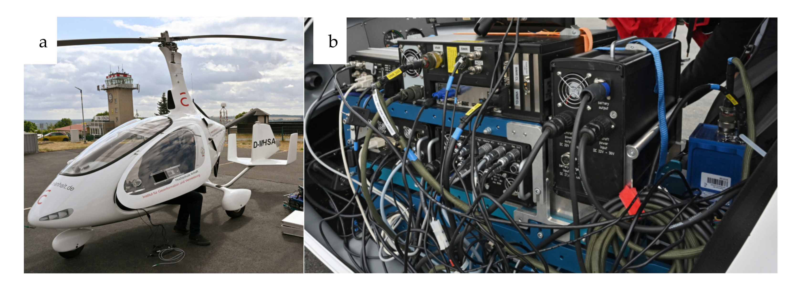
2.2.2. Gyrocopter Measurements

The hyperspectral airborne data were obtained with a HySpex VNIR 1600 camera manufactured by the Norwegian company Norsk Elektro Optikk (NEO), mounted onboard a gyrocopter (see Figure 5). The acquisition range of the camera was λ = 400–1000 nm. In accordance with the flight plan, the hyperspectral data had a spatial resolution of 0.3 m, allowing for a detailed inspection of each tree crown (single-tree level). The HySpex camera acquired the hyperspectral data on 80 bands with a spectral resolution of approximately 7.4 nm. The more narrow the bands, the higher the ability to spot the differences in spectral reflectance between healthy trees and the ones at the beginning stage of pest infestation. Both study areas were observed during the flight campaign (see Figure 1 and Figure 2).
Dodgy weather conditions during the flight caused changes between cloudy and sunny periods. This means the weather was mostly sunny with a few scattered clouds, with both study areas being cloud-free at the time of data acquisition. Nevertheless, the spectral data needed a thorough atmospheric correction during preprocessing.
In addition, a Nikon D800e was mounted on board of the gyrocopter, with which orthophotos with a spatial resolution of 10 cm and 30 cm as well as a digital surface model (DSM), resampled to a spatial resolution of 12 cm, were created for both study areas.
The orthophoto used for the analysis of the second study area was acquired on 22 September 2019, has a spatial resolution of 20 cm and comes from Google Earth.

2.3. Methodology

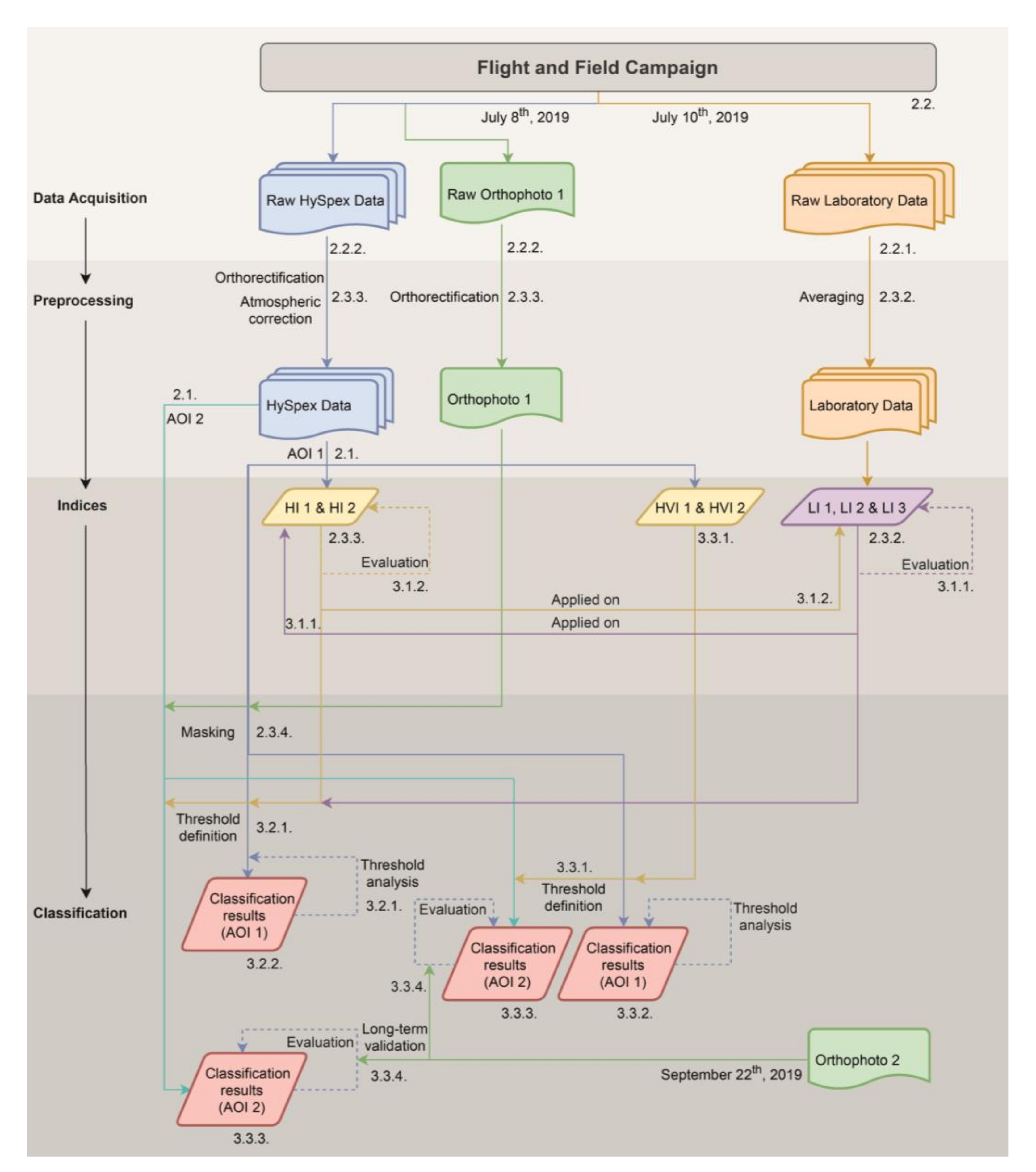
2.3.1. Methodological Design

The most important methodological steps including the associated sections of this work are shown in Figure 6. Basically, airborne and field hyperspectral data as well as orthophotos were acquired during a flight and field campaign. These data were preprocessed accordingly. Subsequently, indices for the first study area were generated based on both airborne and field hyperspectral data. These indices were applied to both types of data, compared with each other, and the index with the highest accuracy to distinguish between healthy and infested spruces was selected. This index was applied to both study areas for classification, using orthophotos from July as reference. The classification results for the first study area (AOI 1) were validated with field samples, while an external orthophoto from September was used for a long-term validation of the second study area (AOI 2).

2.3.2. Processing of the Field Measurements

Data Preprocessing

For a combined interpretation of the field measurements and aerial data, a preprocessing of the hyperspectral field data to the level of absolute reflectance factors is necessary. A corresponding preprocessing algorithm comprising the following four main steps was implemented in the programming language R [41]: (1) transform ASD data into ASCII format; (2) perform linear interpolation between successive white reference measurements; (3) compute reflectance factors based on the corrected white reference data; (4) computation of statistical metrics for each needle sample.
The second processing step was carried out to compensate for small deviations from the instrument calibration that appear during the measurement process (e.g., due to sensor drift or changes in the illumination conditions). The digital numbers (DNs) of the white reference measurements acquired before and after the target measurements were compared. Based on the assumption that the detected changes happened linearly, synthetic white references were generated by wavelength-dependent linear interpolation between the DNs of consecutive white reference measurements. In the third step, the synthetic white reference was deployed to retrieve relative reflectance factors for each sample. Occurring offsets in the relative reflectance factors between the three FS3 sensors were removed by adapting the relative reflectance factors of the VNIR (λ = 350–1000 nm) and SWIR2 (λ = 1801–2400 nm) sensor to the level of SWIR1 (λ = 1001–1800 nm) relative reflectance factors. Afterwards, the relative reflectance factors were multiplied with the reflectance of the Spectralon reference panel to retrieve absolute reflectance factors (ARF) [42]. In the fourth step, various statistics were subsequently computed based on the average of the ten measurements of each sample.
In particular, we visualized the absolute reflectance factors for the different trees, for the different positions (“OA”, “OJ”, “UA” and “UJ”; see Figure 3), as well as the average ARFs of healthy and infested tree samples, separately (see Figure 7). Figure 7a illustrates that T5 is characterized by much lower ARFs than the other trees, due to its discoloration. In Figure 7b, the ARFs for healthy (“G”) and infested (“K”) trees are averaged for λ = 350–2500 nm, depending on the sample positions (“OA”, “OJ”, “UA” and “UJ”). T5 was ignored, since the not typical reflectance for the early infestation phase would distort the averaged ARF. As the aerial hyperspectral data were acquired for λ = 400–1000 nm only, the following analysis considers only this wavelength range.

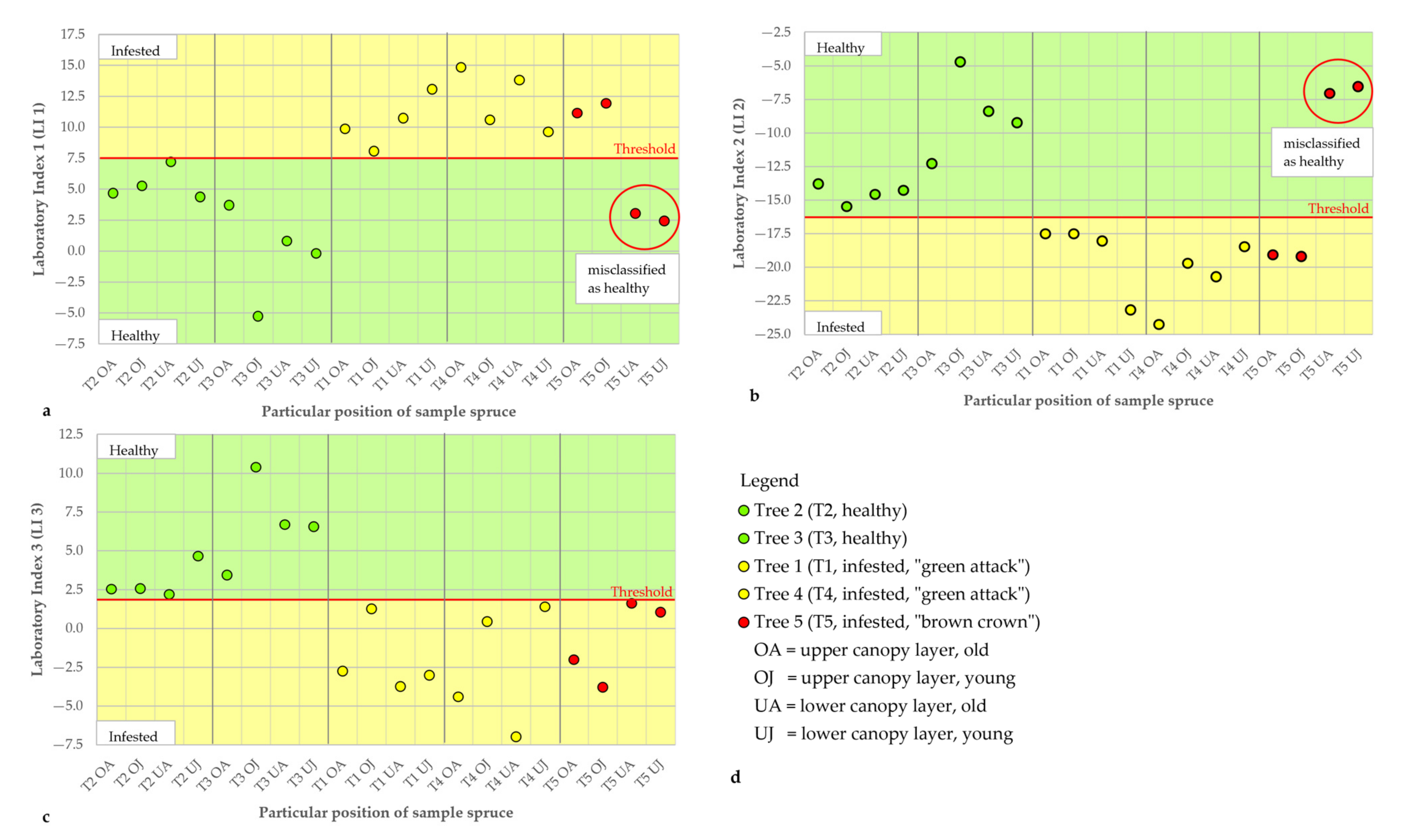
Laboratory Indices (Field Data)

One aim of this work is to determine a suitable index for the detection of early bark beetle infestation (green attack). In a first step, we tried to find a suitable index based on laboratory data.
The red-edge domain is particularly important to distinguish between infested and healthy spruces [29]. Figure 7a shows that the mean reflectivity of the needles of infested trees (green attack) show a slightly rounded signature at the end of the red-edge domain (approximately 750 nm) compared to healthy trees, regardless of the considered position of the needle samples (see Figure 3) on the tree. However, this tendency cannot be confirmed if the healthy and infested spruces are not averaged.
For this reason, in this preliminary study, we have defined indices based not only on this slightly rounded signature, but also on other properties of the red-edge spectrum, i.e., a region of the spectrum closer to the red and visible part (see Table 2).
There were very small differences between the examined positions of all sample spruces, which were also not uniform for the respective degree of infestation. In order to enhance these differences and be able to better distinguish between infested and healthy spruces, only the parts of the spectrum where these differences are more significant are considered. For this purpose, the difference between adjacent wavelengths, several parts of the spectrum and various combined weightings of these parts were used.
Following this approach, we have defined three laboratory indices (LI 1–3) that can distinguish between infested (green attack) and healthy sample spruces (see Table 2). Since the spectral resolution of the HySpex data is 7.4 nm (see Section 2.2) and that of the laboratory data is 1 nm, the laboratory data and therefore also the LI were adjusted to the wavelengths of the HySpex data in order to be able to apply the LI to the HySpex data later (see Section 3.1.1). It is important to note that the ASD Fieldspec only records integer wavelengths and thus a maximum deviation of 0.5 nm can occur between the two data sources.

2.3.3. Processing of the Hyperspectral Data

Processing Atmospheric Correction with Py6S Algorithm

Both the HySpex data and the orthophoto were orthorectified after acquisition. An atmospheric correction was then applied to convert radiance into reflectance values. Due to the lack of calibration tarps, we performed the correction using the Python package Py6S [43], an interface to the 6S radiative transfer model [44]. Unlike commercial software, Py6S is open source and allows for more flexible parameter tuning using Python scripts. Moreover, this fine-tuning is easier and faster to perform, and the analysis is more reproducible.
The flight campaign was conducted in alternating cloudy and sunny conditions, and gaps in the metadata made atmospheric correction difficult. Nevertheless, the cloud-free conditions in both study areas allow an application of the atmospheric correction with Py6S. Certain model parameters required for the Py6S algorithm, such as the view zenith angle, were estimated and others, such as the solar zenith angle and solar azimuth angle, were derived from other sources [45].

HySpex Indices (Airborne Data)

As mentioned in Section 2.3.2, one aim of the work is to determine a suitable index for the detection of early bark beetle infestation (green attack). In a second step, we have therefore tried to find a suitable index based on the atmospheric corrected hyperspectral airborne data. In fact, we found two HySpex indices (HI 1–2) that can distinguish between infested and healthy spruce (see Table 2).
As suggested by Lausch et al. [22] and Abdullah et al. [23], we mainly focused on the red-edge range 680 to 750 nm for the definition of the indices. In addition, we specifically considered the flattening effect of infested spruces (see Figure 7, red arrow) in the red-edge. Complex methods such as partial least squares (PLS) or various machine learning methods could be investigated for this purpose. However, on the one hand, the sample size is too small for a suitable training of machine learning methods and on the other hand, there is the risk that the results are difficult to interpret. Therefore, to keep the HySpex indices simple, only two wavelengths are used, representing the increase in red-edge reflectance. The steeper this increase, the less likely is a bark beetle attack.
The analysis of the hyperspectral data was performed in ENVI version 5.5.

2.3.4. Classification

Based on the defined indices, we performed classification of the airborne hyperspectral data in order to detect infested trees in the green attack phase.

Masking

To reduce unnecessary information prior to classification, we masked all pixels that did not represent spruce canopies. For this approach, we used a Spectral Angle Mapper (SAM) classification specifically designed for high-dimensional data, such as the hyperspectral HySpex data used here. Ambiguous objects or pixels identified during the field campaign of the classes deciduous trees, spruces, soil and grassland were used as training pixels for the SAM classification. To additionally distinguish between deciduous and spruce trees, we used high-resolution orthophotos to consider the canopy structure.
Trees with sparse crowns or edge pixels of the canopy are particularly prone to mixed pixels. We reduced this problem by masking the edge pixels of the spruces and considered only central pixels of denser crowns. To achieve this, we examined the crown structure from high-resolution orthophotos for each spruce in both study areas. By masking the edge pixels in the later processing stages, the effect of self-shadowing of the spruces can also be reduced.

Threshold Based Classification Approach

After masking, we applied the index that best distinguishes between infested and healthy spruces to the atmospherically corrected HySpex data. Using threshold values, one class is formed for healthy and two for infested spruces. Central pixels of sample spruces and the adjacent infested spruces with a brown crown were taken into account.
The suitable threshold values are determined with the help of a threshold value analysis (see Section 3.2.1). Thereby, we examined the variations of the overall accuracy (OAA) for all central pixels of T1–3 for different threshold values (see Section 3.2.1). The central pixels of T1–3, which serve as a reference, were manually classified as healthy or infested based on the information obtained during the field campaign.
To test the transferability of the best index, it was applied to the second study area (see Section 3.3.3). As there is only one sample spruce (T4) with an unknown position in this area, a validation was performed with another high-resolution orthophoto acquired a few months later. Based on the bark beetle’s life cycle according to observations by ThüringenForst, a spruce loses large amounts of green needles one month after the first infestation (green attack). After about 6–10 weeks, shortly before or even after the next bark beetle generation flies out, the tree crown gradually turns brown (gray attack) (see Section 1.1). Therefore, spruces classified as infested by the best index should show typical crown discoloration a few weeks later, which can be roughly validated using the second orthophoto, based on a comparison with reference brown crown spruces. This ensures a long-term validation of the classification results (see Section 3.3.4).

3. Results

In this section we first compare all laboratory indices (LI 1–3) with the field laboratory data and then all HySpex indices (HI 1–2) with the airborne hyperspectral data, and analyze their transferability to the respective other database (see Section 3.1). In this, we investigated whether one of these five indices is suitable for both types of data. Subsequently, we used the best index to detect an early bark beetle infestation for classification of the airborne data (see Section 3.2). Finally, the robustness of the best index was examined by comparing it with other suitable indices, applying it to the second study area and performing a long-term validation (see Section 3.3).

3.1. Indices

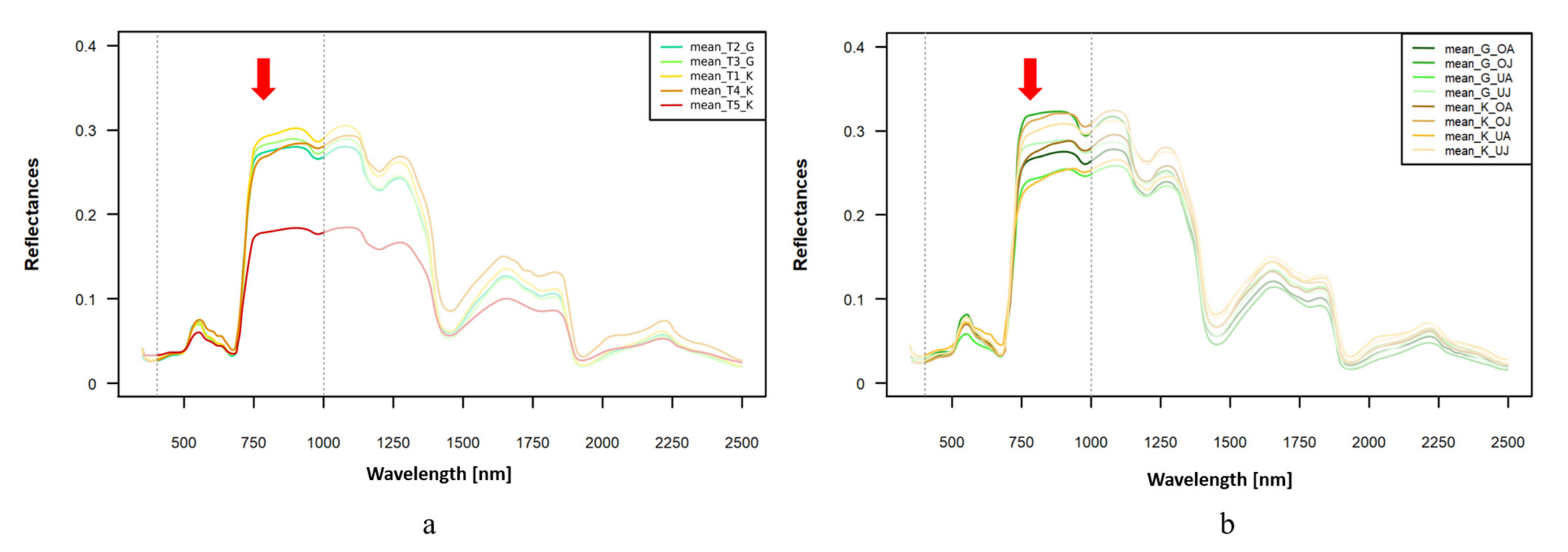
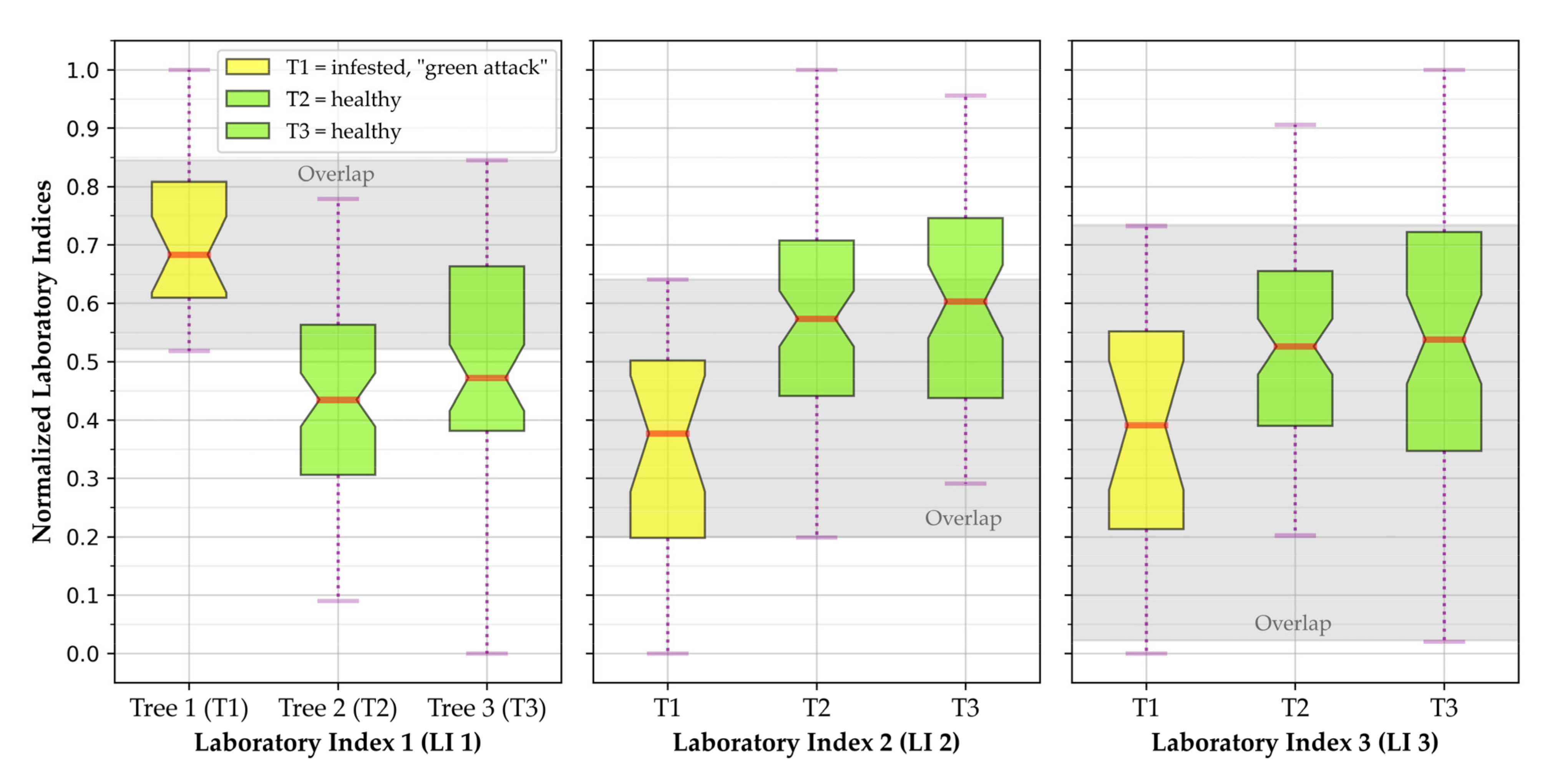
3.1.1. Field Measurements

If the laboratory indices (LI1 1–3, defined in Table 2) are applied to the laboratory data, LI 1–3 can distinguish well between infested (green attack) and healthy needle samples by setting a threshold value (see Figure 8, Table A1, Appendix A). However, two of them (LI 1 and LI 2) cannot correctly classify infested spruce samples (brown crown) because T5 UA and T5 UJ are wrongly classified as healthy. In contrast, LI 3 can distinguish between infested (green attack and brown crown) and healthy spruces.
To compare the performance of the three laboratory indices on the airborne data, we defined different scenarios for the influence of the needles (see Table 3) situated on the different part of the trees (OA, OJ, UA and UJ, see Figure 3). The normalized index values averaged for all tree positions are shown in Table A1, together with the normalized distance between the infested and healthy tree values. For the first scenario, it is assumed that a pixel consists of OA, OJ, UA and UJ in equal proportions, i.e., the mean value is calculated. In contrast, the ratio 40:40:10:10 was chosen for the second scenario. Especially, with airborne data, it is expected that the needles situated on the top of the crown (OA and OJ) have a higher influence on the spectral signature than needles situated on the lower parts of the canopy, due to the dense tree canopy being visible in the first orthophoto (see Figure 1). The third scenario was expanded by the assumption that younger branches are mainly found at the edge of the tree, and are therefore less relevant for the central pixels. Hence, the ratio 33:27:22:18 was chosen for the third scenario, which also takes UA and UJ into account more than second scenario.
In all three scenarios, the smallest normalized distance between infested (green attack) and healthy needles is significantly greater for LI 3 (mean: 0.52) than for LI 1 (mean: 0.39) and L2 (mean: 0.34) (see Table A1). However, if infested spruce needle samples (brown crown) are taken into account, this difference drops drastically for LI 1 (mean: 0.2) and LI 2 (mean: 0.06), but not for LI 3 (mean: 0.44). This means that LI 3 is less prone to misclassification than LI 1 and LI 2 due to this larger difference.
Overall, LI 3 proved to be the most suitable for classifying the needles of the sample spruces measured in the laboratory as infested and healthy.
If, in a next step, LI 1–3, which worked well for the laboratory spectra, are applied to the atmospherically corrected HySpex data, a distinction between infested and healthy sample spruces is no longer clearly possible. When comparing the laboratory indices, there is a large overlap (grey area), especially for LI 3, between infested and healthy sample spruces (see Figure 9). This means that no suitable threshold can be found to differentiate between healthy and infested spruce. Accordingly, the laboratory indices can only be used to a limited extent to differentiate between healthy and infested spruces in the airborne data.

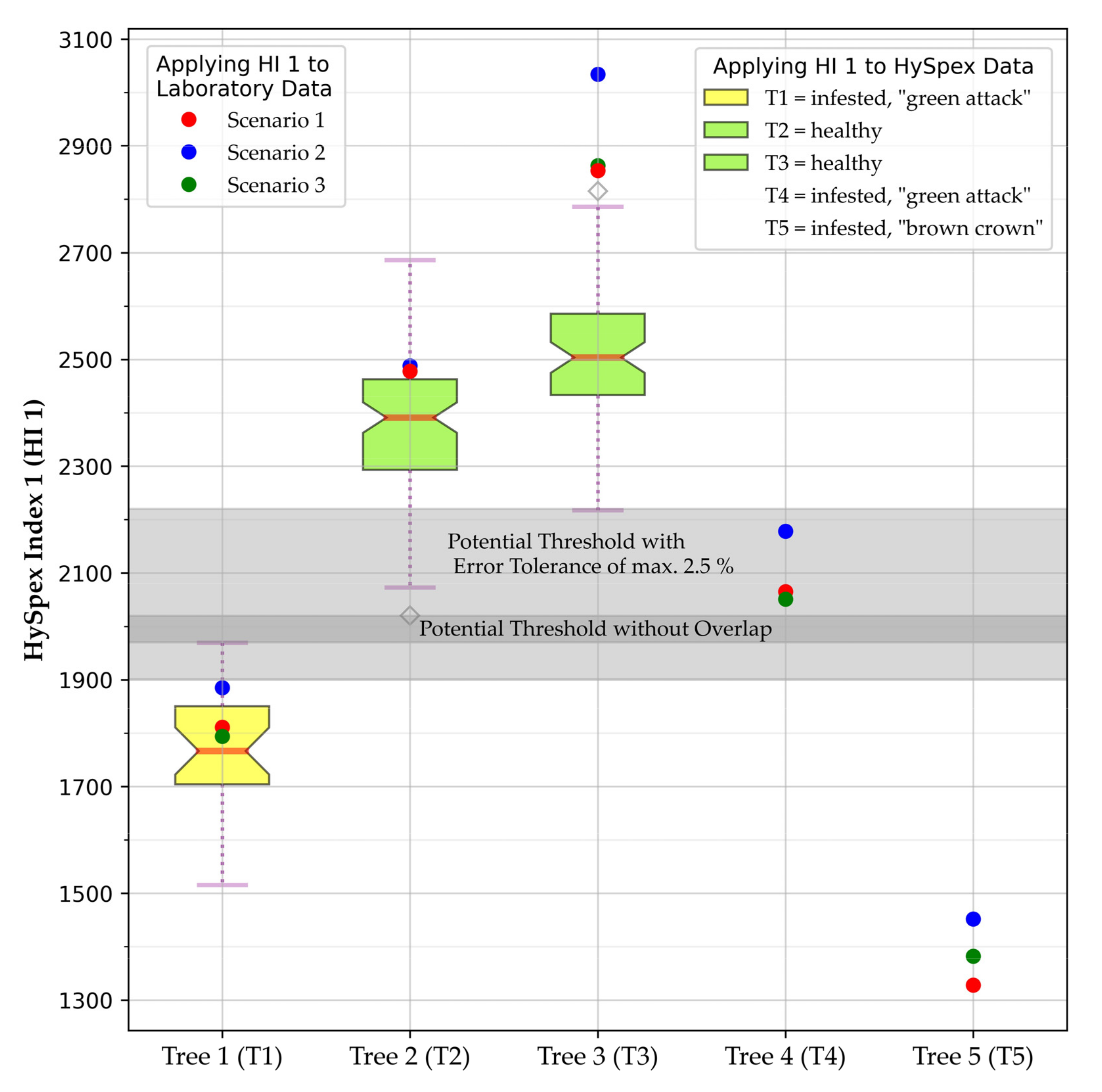
3.1.2. Hyperspectral Data

In order to compare HI 1 with HI 2, the values of the sample spruces in the atmospherically corrected HySpex data of both indices were normalized and then compared. These normalized values can be found in Table A2. Because only the position of T1–3 is known, only these spruces have been taken into account. When comparing the normalized 5th and 95th percentiles of both indices, the normalized distance between infested and healthy spruce is higher for HI 1 (0.26) than for HI 2 (0.21) (see Table A2). This means that HI 1 was less prone to misclassification than HI 2. Nevertheless, both indices were suitable for differentiating between healthy and infested spruce for the HySpex data.
When HI 1 and HI 2 were subsequently applied to the laboratory field data, HI 1 performed significantly better than HI 2. The scenarios defined in Table 3 were used to calculate the normalized weighted mean values of the indices per tree (see Table 4). If the normalized distance between healthy (T2 and T3) and infested (T1 and T4) spruces was calculated, there was a positive difference for HI 1 (see Table 4, last column). This means that there was no overlap between healthy and infected spruces and therefore a suitable threshold can be defined to differentiate between healthy and infected spruces. In contrast, HI 2 had a negative difference (red numbers in Table 4). This means that HI 2 cannot differentiate between healthy and infested spruces, when applied to the laboratory data, due to an overlap of both classes. Consequently, only HI 1 was used for further analysis.
Whilst HI 1 seems to be able to distinguish between healthy and infested spruces when averaging all tree positions together (“OA”, “OJ”, “UA” and “UJ”), the behavior of this index for a particular position does not provide sufficient information to distinguish which part of the tree may be already infested.
HI 1 was able to distinguish between healthy and infested spruce when applied to both the HySpex data and the laboratory data. A comparison when applying HI 1 to the laboratory data and HySpex data is shown in Figure 10. This allowed the three mix-pixel scenarios (see Table 3) to be evaluated. For this purpose, HI 1 was first applied to the laboratory data of the respective sample spruce and a weighted mean value per spruce was calculated on the basis of the scenarios (red, blue, green dot). This weighted mean was then compared with the median of the individual sample spruce in the atmospherically corrected HySpex data (50th percentile line). The closer the mean value of a scenario was to the median, the more realistic the scenario was. However, possible remaining measurement errors in laboratory data (see Section 2.2.1) and gyrocopter data acquisition (see Section 2.2) can influence these results.
It is noticeable that the normalized mean values of the three scenarios of the HySpex data moderately to very strongly overestimated the application of HI 1 to the laboratory data (see Figure 10). While two of the three mean values of the scenarios of T1 lie between the 50th and 75th percentile of the HySpex data, only one scenario does so for T2. For T3, the mean values are outside the 5th and 95th percentiles, but close to the 100th percentile (2816). This means that especially very high values of HI 1, as present in the vital T3, are strongly overestimated. However, this error can be neglected, as only the lower threshold value of T2 is relevant for the distinction between infested and healthy spruces (see grey bars).
Furthermore, especially the second scenario overestimated the median of T1 and T3, while scenarios 1 and 3 led to quite similar weighted mean values.
Although numerical measurements of T4 and T5 are not available due to the unknown position, these can be estimated using the laboratory spectra in combination with the scenarios. Accordingly, the median of T4 (HySpex data) could be between T1 and T2, while the median of T5 is lower than that of T1.
Overall, the laboratory spectra in combination with the scenarios overestimated the atmospherically corrected HySpex data, but the scenarios for T1 and T2 still fit well, but not for T3.
To sum it all up, of all laboratory and HySpex indices, HI 1 was the index that could best differentiate between healthy and infested spruces for the atmospherically corrected HySpex data. Consequently, HI 1 was used for the classification (see Section 3.2).

3.2. Classification for HySpex Index 1

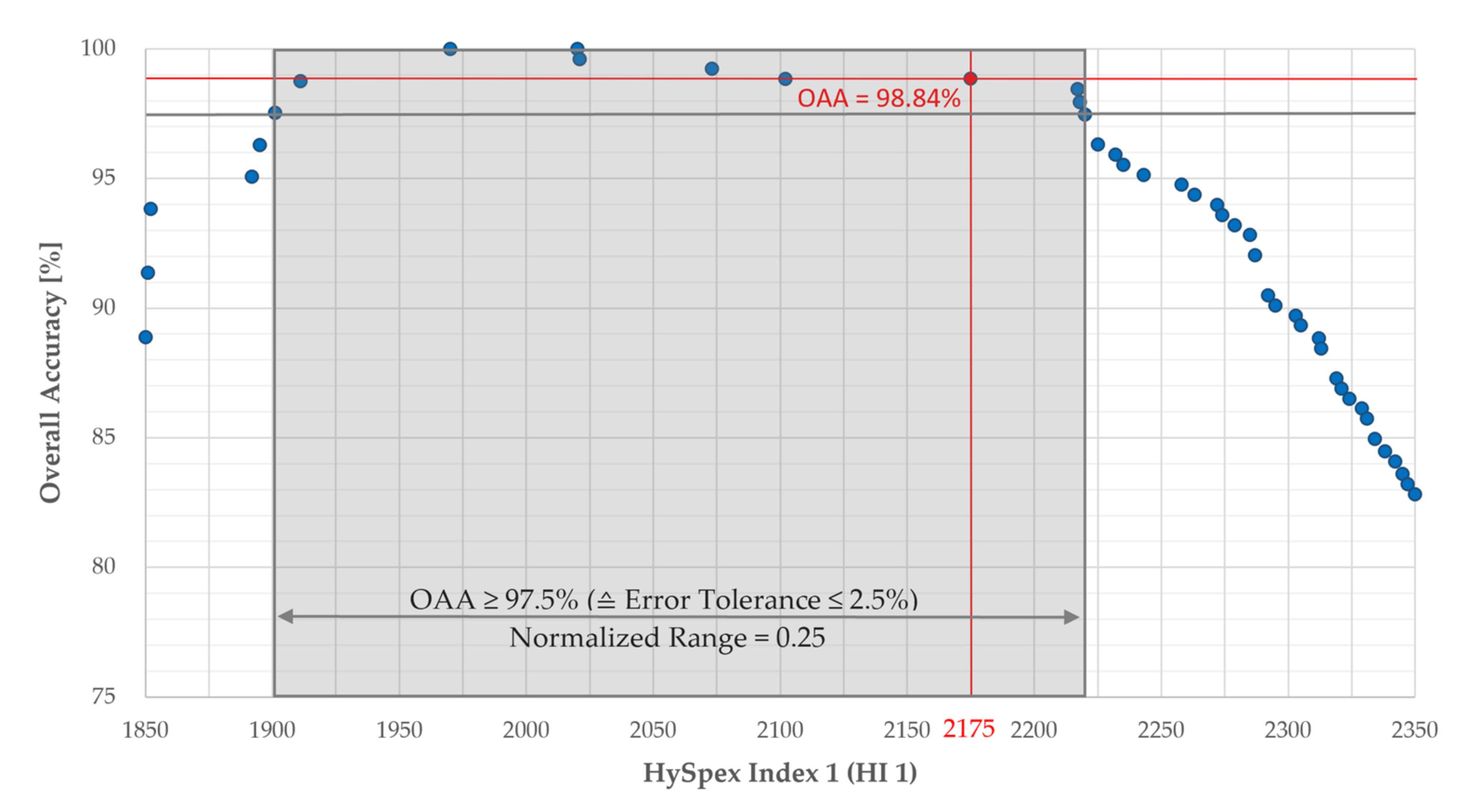
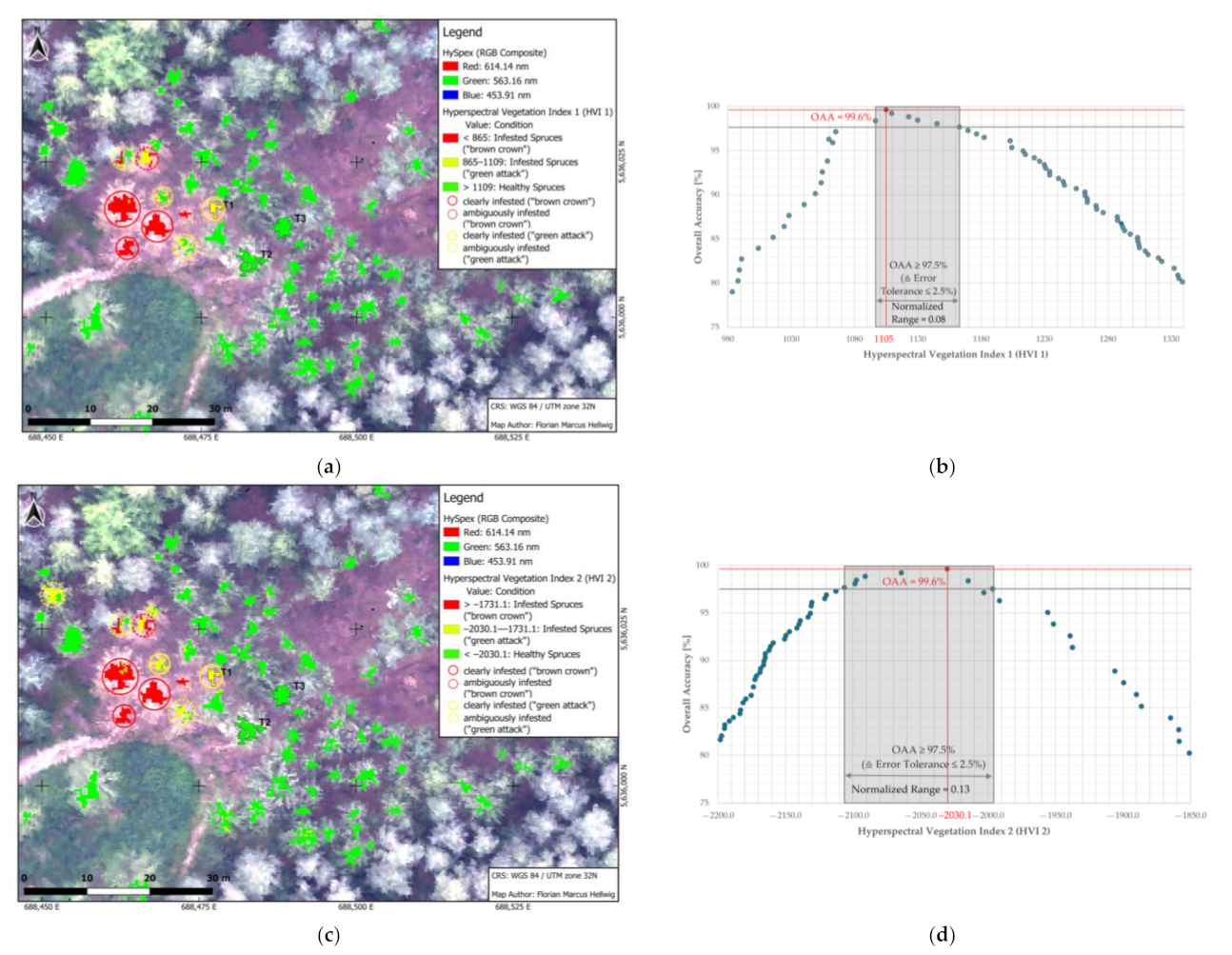
3.2.1. Threshold Estimation (Study Area 1)

As a result of the analysis of various indices in the last section, HI 1 is by far the best to distinguish between infested and healthy needles of the sample spruces both for the HySpex data and for the laboratory spectra. Therefore, we applied HI 1 to the entire first study area and analyzed the classification results in more detail.
The threshold for differentiating between infested spruces in the early (green attack) and late stage (brown crown) was determined on the basis of the unambiguous infested spruces with brown crowns (see Figure 1, west of T1–3). Since the fifth percentile of T1 is also close to 1550 (see Figure 10), we set this threshold to 1550. Nevertheless, this threshold cannot be validated appropriately and is therefore only an estimation.
To determine the optimal threshold for HI 1 distinguishing between infested (green attack) and healthy spruces, we performed a threshold analysis. This also enables a general validation of the classification results (see Section 3.2.2 and Figure 11).
Taking into account all central pixels of T1–3 (181), a threshold between 1970 and 2020 led to an overall accuracy (OAA) of 100% (see Figure 12). The OAA was calculated by dividing the number of correctly classified pixels by the number of all central pixels. By increasing the error tolerance to a maximum of 2.5%, the range of values for a potential threshold increased significantly to 1911–2220 (OAA ≥ 97.5%). A further increase in the error tolerance to 5% only slightly enlarged the range of the optimal threshold value (1892–2243). It must be noted here that, due to its size, T1 contains significantly fewer pixels (27) than T2 (86) and T3 (68), and therefore has a lower overall influence on the OAA.
Considering that the values of HI 1 of T4 are between those of T1 (infested) and T2 (healthy) (see Figure 10), it was advisable to set the threshold value higher. Therefore, we adjusted the threshold value for distinguishing between infested and healthy spruces to 2175 to find a compromise from the previous results. This means that there was a risk that healthy pixels were wrongly classified as infested.

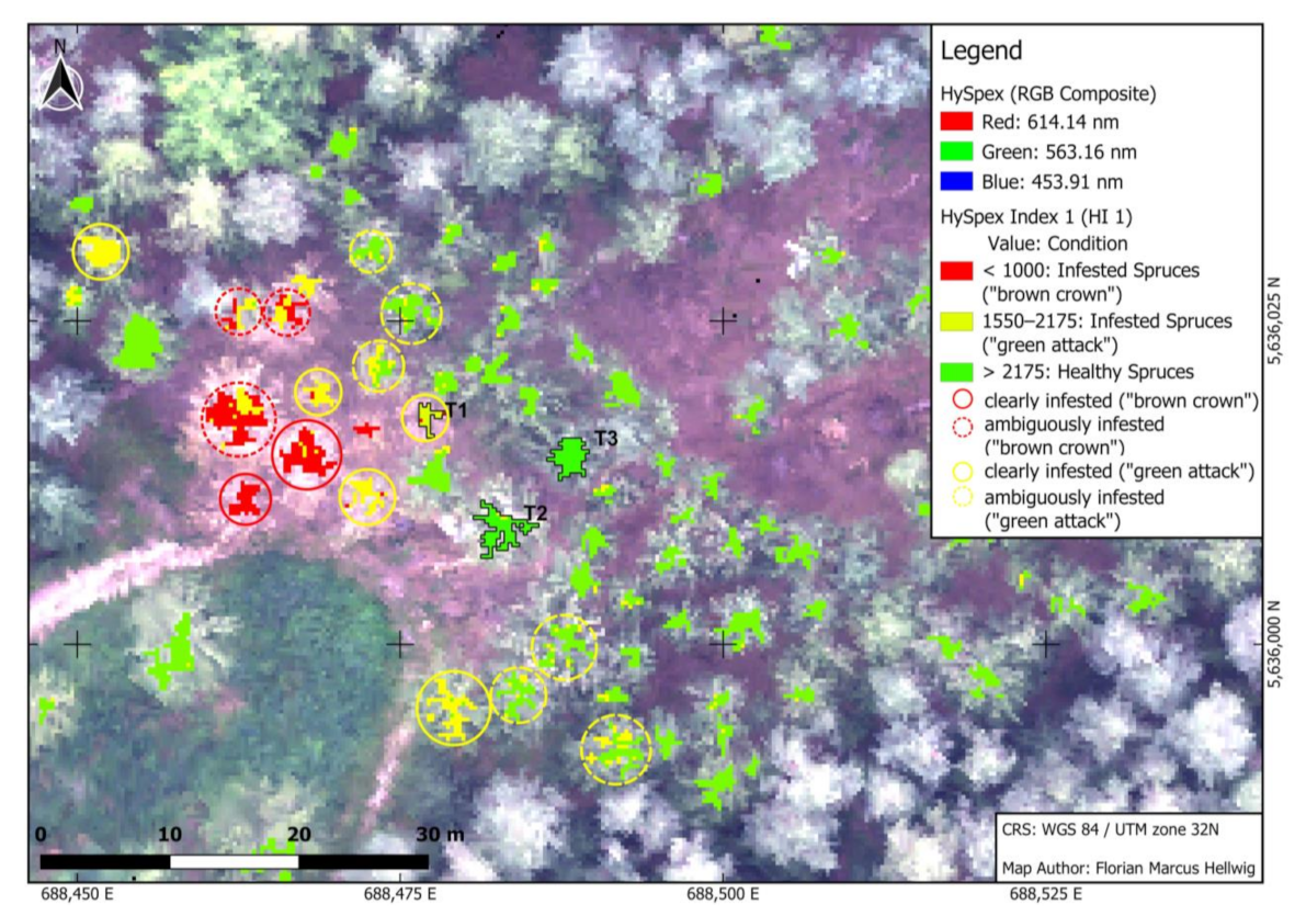
3.2.2. Classification Results (Study Area 1)

After applying HI 1 with the adjusted threshold values defined in Section 3.2.1 to the entire first study area, it is possible to classify all spruces (about 80 trees) (see Figure 11). As mentioned in Section 2.3.4, only the central pixels of the spruces were considered. It corresponded to an area of about 3002 pixels or 270.18 m2, depending on the considered tree. Due to the low number of pixels in spruces with a small crown, a clear distinction between infested and healthy was not always possible. Therefore, only spruces with a crown larger than 22 pixels (>1.98 m2) were considered. Due to subjective errors in the selection of the central pixels and the adjusted threshold (see Section 3.2.1), a classification was only considered unambiguous from 90% of a class.
Overall, six spruces were unambiguously infested (green attack, dotted yellow circle), five spruces were infested (green attack, yellow circle), three spruces were unambiguously infested (brown crown, dotted red circle) and two spruces were infested (brown crown, red circle). It is also worth mentioning that infested spruces usually do not appear individually, but in groups.
To validate this classification, we used threshold analysis again (see Figure 12). The threshold value of 2175 resulted in a very good OAA of 98.84%, with T1 and T3 correctly classified as infested or healthy by 100%.

3.3. Transfer of HySpex Index 1

As mentioned in the last section, HI 1 can differentiate very successfully between infested and healthy spruces. To test the transferability of HI 1, common indices for bark beetle detection were defined (see Section 3.3.1), tested and compared with HI 1 in both study areas (see Section 3.3.2 and Section 3.3.3). An external second orthophoto of the second study area enabled the long-term validation of HI 1 and the other indices (see Section 3.3.4).

3.3.1. Investigation of Other Suitable Indices

Lausch et al. [22] and Abdullah et al. [23] have found that there are several indices that can be used to distinguish between infested and healthy spruces. After applying the indices for the wavelength range 417–992 nm to the atmospherically corrected HySpex data, two hyperspectral vegetation indices (HVI 1 and HVI 2) turned out to be promising. These spectral derivatives defined by Lausch et al. [22] were adapted to the HySpex wavelengths and are listed in Table 2.

3.3.2. Comparison of HySpex Index 1 with Other Suitable Indices (Study Area 1)

Using the threshold analysis approach from Section 3.2.1 (see Figure 13b,d), the threshold value between infested and healthy spruces was set to the value with maximum overall accuracy (HVI 1: 1109 and HVI 2: −2030.1). The lowest or highest value of the respective index of T1 was set as the threshold value from infested (green attack) to infested (brown crown) (HVI 1: 865 and HVI 2: −1731.1). The classification results for the first study area based on these threshold values are also shown in Figure 13a,c.
If only spruces with a crown larger than 22 pixels (>1.98 m2) were considered, using HVI 1, three spruce were unambiguously infested (green attack, dotted yellow circle), one spruce was infested (green attack, yellow circle), one spruce was unambiguously infested (brown crown, dotted red circle) and three spruce were infested (brown crown, red circle) (see Figure 13a). Apart from the spruces that were removed, no spruces were classified as infested (green attack).
In contrast, using HVI 2, three spruces were unambiguously infested (green attack, dotted yellow circle), two spruces were infested (green attack, yellow circle), one spruce was unambiguously infested (brown crown, dotted red circle) and three spruces were infested (brown crown, red circle) (see Figure 13c). Apart from the removed spruce, one large spruce in the northwest was classified as unambiguously infested (green attack). However, this spruce was classified as healthy for HVI 1. HVI 2 therefore finds more infested spruces than HVI 1, which leads to a slightly different classification.
When evaluating the accuracy assessment, it was noticeable that both indices can achieve the same, very high level of accuracy (99.61%) (see Figure 13b,d). Both indices can classify T1 and T3 with 100% accuracy, but not T2. However, the normalized span of the range of values where both indices have an accuracy of more than 97.5% was greater for HVI 2 (0.13) than for HVI 1 (0.08). This means that HVI 2 had more possibilities to set an appropriate threshold.
Overall, HVI 2 appeared to be slightly superior to HVI 1. However, both indices had the same very high accuracy.
When HVI 1 and HVI 2 are compared with HI 1, all three indices detect the same eight larger infested spruces and have a similar very high OAA (≥98.84%). It is also noticeable that HVI 2 and HI 1 both identify the same infested spruce (northwest), which was not removed later, that HVI 1 does not. HVI 2 detected the beginnings of an infestation (<10%) in the same three spruces as HI 1 (northwest of T1 and in the south), although HI 1 classified them as ambiguously infested (green attack) (≥10%). HI1 also recognized more (ambiguously) infested spruces overall (16) than HVI 2 (9) and HVI 1(8), four of which (north of T1 and in the south) were only classified as infested in a small proportion (<20%).

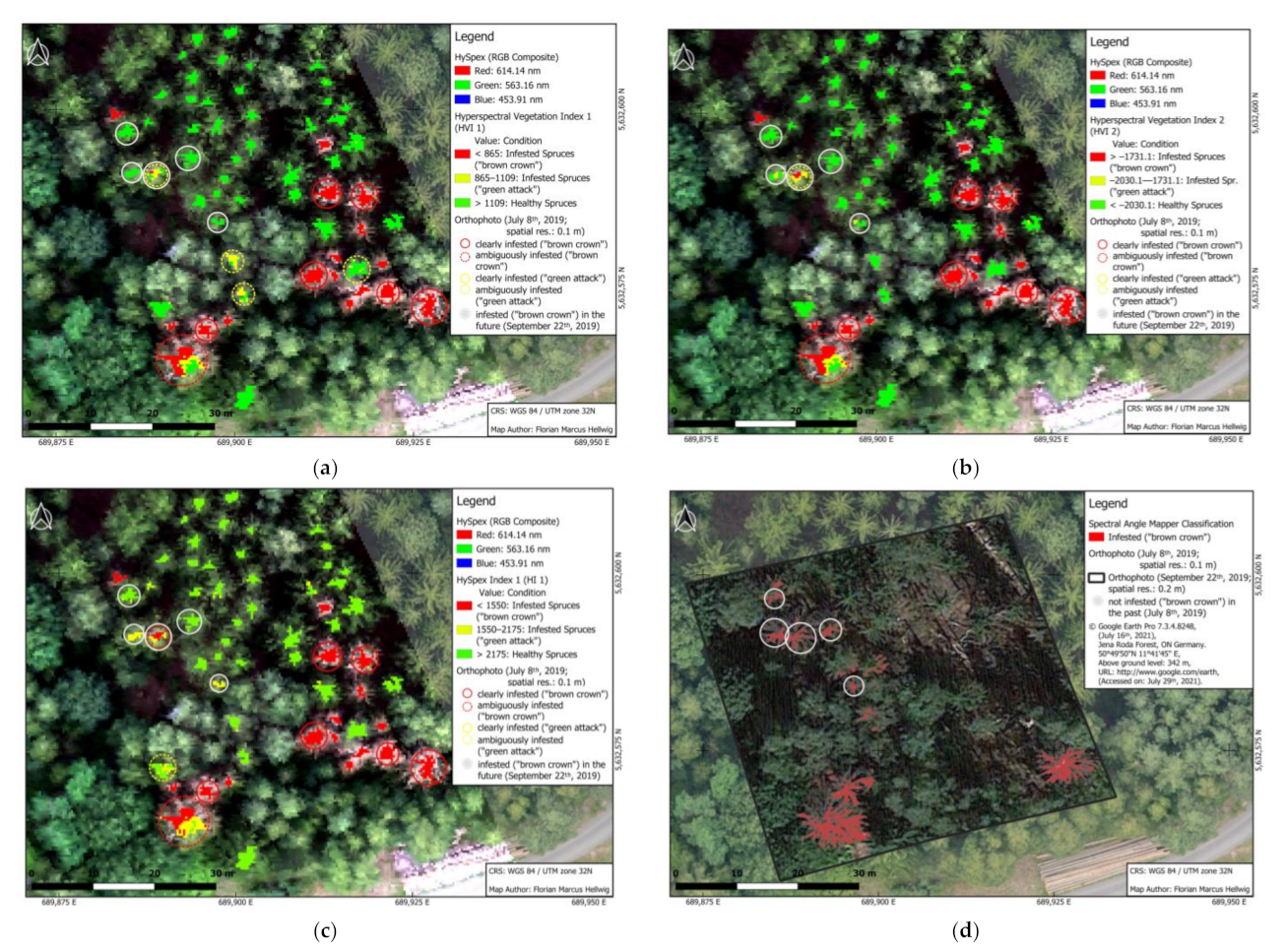
3.3.3. Comparison of HySpex Index 1 with Other Suitable Indices (Study Area 2)

To further test the transferability of HI 1, it was applied to the second study area (see Figure 14c) and compared to the suitable HVI 1 (see Figure 14a) and HVI 2 (see Figure 14b).
As for the first study area, the spruces in the second study area were classified according to the same minimum pixel size and threshold values for HVI 1 and HVI 2 as defined in Section 3.3.2, and for HI 1 in Section 3.2.1, respectively. In the second study area there were about 60 spruces, which corresponded to an area of about 1432 pixel or 128.88 m2. For HVI 1, four spruces were unambiguously infested (green attack, dotted yellow circle), one spruce was unambiguously infested (brown crown, dotted red circle) and six spruces were infested (brown crown, red circle) (see Figure 14a). For HVI 2, on the other hand, only one spruce was unambiguously infested (green attack, dotted yellow circle), one spruce was unambiguously infested (brown crown, dotted red circle) and six spruces were infested (brown crown, red circle) (see Figure 14b).
When comparing these two classification results, it is worth mentioning that on the one hand both indices detected the same spruces in the same infestation stage. On the other hand, HVI 1 additionally classified two spruces in the southern center as unambiguously infested (yellow dotted circle), which HVI 2 classified as healthy.
When HVI 1 and HVI 2 were compared again with HI 1, HI 1 classified the same spruces as HVI 2 in an almost identical infestation stage (see Figure 14c). Only the spruce in the northwest (white circle) was classified more as an ambiguous late infestation (brown crown). In contrast to HVI 1 and HVI 2, however, HI 1 classified another large spruce in the southwest as ambiguously infested (green attack, yellow dotted circle) and two small spruces in the northwest (white circles) as infested (green attack). Interestingly, HI 1 recognized other spruces as ambiguously infested than HVI 1.

3.3.4. Long-Term Validation of HySpex Index 1 and Other Indices (Study Area 2)

To ensure long-term validation of the second study area, we used an external orthophoto from 22 September 2019. Due to the life cycle of bark beetles according to observations by ThüringenForst, typical canopy discoloration occurs no earlier than around 6–10 weeks after the initial infestation. Since there were 76 days between the day of acquisition of the HySpex data and the external orthophoto, the infested spruces (green attack) in the classification result must be clearly recognizable by a brown crown in the external orthophoto. Due to this time lag, however, it is possible that the spruces were only infested after the HySpex data collection. This means that the spruces were healthy on 10 July but infested (brown crown) on 22 September. A conclusion from the infestation status in the second orthophoto to that of the first was therefore only possible to a limited extent. On the other hand, a spruce that was infested (green attack) in the first orthophoto must inevitably be infested (brown crown) in the second.
Based on the clearly identified pixels of infested spruces (brown crown) detected as such during the field campaign, a SAM classification was used to identify additional, similar pixels (see Figure 14d). After the field campaign in July, almost all of the infested spruces were removed, only two spruces in the southwest and one in the southeast remained in place. The crowns of these large spruces were classified as infested (brown crown) according to the SAM classification. Because these three spruces were clearly classified, this proves the applicability of this SAM classification. In addition to these three spruces, five spruces in the northwest and one in the center were also clearly classified as infested (brown crown) (white circles). Since one of these spruces (northwest), like the three previously mentioned spruces, was already obviously infested (brown crown) at the time of data acquisition in July, this spruce was not considered further. Furthermore, not taken into account were the spruces that were ambiguously infested in the SAM classification (two spruces in the center).
If HVI 1 and HVI 2 are long-term validated, HVI 1 recognizes only one out of five spruces in an early infestation stage (green attack) (white circle), while HVI 2 also detects only one out of five spruces, but in addition detects the tendency to infestation in two spruces. However, HVI 1 still identifies two spruces in the center as unambiguously infested (yellow dotted circle), which were classified as ambiguously infested in the second orthophoto. Due to the time lag between the two orthophotos, however, these spruces should be definitely infested (brown crown). Since this is not the case, HVI 1 overestimated the bark beetle infestation accordingly. Additionally, HVI 1, in contrast to HVI 2, did not recognize at least the beginning of the infestation. Consequently, HVI 2 in combination with the chosen threshold can detect the bark beetle infestation more effectively than HVI 1.
On the other hand, HI 1 detected three out of five spruces in an early stage of infestation (green attack) (white circle), and also at the beginning of an infestation in another spruce (see Figure 14c). It is possible that this spruce and the other spruce not detected were not yet sufficiently infested at the time of data acquisition (10 July 2019). As for HVI 1, there was a (small) risk of overestimating the infestation for HI 1, since HI 1 detected an ambiguously infested spruce (green attack, yellow dotted circle) in the southwest, which was not infested according to the SAM classification. However, since it is only an ambiguous infestation, this error can be neglected and compensated for by adjusting the threshold value.
When comparing all three investigated indices in the long-term validation, HI 1 recognized more spruces (three out of five) in the early infestation stage (green attack) than HVI 1 and HVI 2 (one out of five). Consequently, HI 1 is superior to other suitable indices, such as HVI 1 and HVI 2 for detecting bark beetle infestation at an early stage (green attack).
Overall, HI 1 proves to be robust and superior to the other suitable indices, not only in the first study area (OAA = 98.84%), but also when transferred to another study area and in long-term validation. HI 1 therefore has the potential to detect an early bark beetle infestation (green attack) relatively successfully.

4. Discussion

4.1. Comparison of the Laboratory and HySpex Indices

The laboratory indices (LI 1–3), especially LI 3, work well when applied to the laboratory data (see Section 3.1.1 and Table A1); and the hyperspectral indices (HI 1–2), especially HI 1, work well when applied to the HySpex data (see Section 3.1.2 and Table A2), but not vice versa, except for HI 1.
LI 3 represents on the one hand a combination of LI 1 and LI 2. On the other hand, LI 3, similar to LI 1, uses bands in the green and blue spectrum in addition to the red-edge region to account for photosynthetically-active pigments. The chlorophyll content, represented by chlorophyll absorption (at about 490 nm), can provide information about the presence of bark beetles, as the feeding behavior of the bark beetles impairs the transport of nutrients from the needles to the roots of the infested spruces. This causes a nutrient deficiency in the needles, which is manifested by a chlorophyll reduction [13]. HI 1–2, in contrast, used only the red-edge region. HI 1 produced better results than HI 2 because it considers the area immediately at the edge of the red-edge (731–753 nm), instead of the rise before it (723–738 nm). This allowed HI 1 to fully account for the flattening of the spectral signature at the red-edge, which was also visible in the laboratory data of infested spruces (see Figure 7, red arrow).
However, when the laboratory indices (LI 1–3) were applied to the HySpex data, they could only distinguish between healthy and infested spruces to a limited extent (see Section 3.1.1 and Figure 9). There are many reasons for this. First, in our analysis, 20 needle samples (four positions for five trees) were considered for the laboratory data (see Section 2.2.1). Since there are very small differences between the examined positions within and between the infestation classes, relatively complex indices had to be developed (see Section 2.3.2). This led to the fact that LI 1–3 were strongly adapted to the laboratory data. However, when the scale was increased from needle level (1–2 cm) to the pixel level (30 cm) of the HySpex data, other elements, such as twigs, bark, shadowing effects and the underlying vegetation and soil were included. An averaging of all these spectral signatures took place and additional BRDF effects occurred. This caused the differences in the laboratory data between the needle samples to disappear. Furthermore, we analyzed the needle samples under laboratory-like conditions, clumping the needles on the turning table to extract a needle spectrum that corresponds to a theoretical spectrum of the needles only. The laboratory indices were likely to be too fine-tuned, and therefore only transferable to the HySpex data to a limited extent.
HI 1 was again superior to LI 1–3 in application to the HySpex data because of its simplicity. Despite this simplicity, HI 1, when applied to the laboratory data, could distinguish the averaged needle samples well, unlike HI 2. However, without averaging the needle samples, certain individual needle classes could not be correctly classified. For detecting early bark beetle infestation, overall LI 3 was best at the needle level when considering individual needles, and HI 1 was best at the pixel level when considering mixed signatures of spruce elements. It would be worthwhile in the future to measure spectral signatures from branches with needles the size of the spatial resolution of the HySpex data instead of or in addition to individual needles.

4.2. Composition of the Crown Structure

The central pixels of T2 probably consisted of fewer needles from the lower positions (“UA”, “UJ”, see Figure 3) than T1 and T3 (see Figure 10).
Assuming that the bias due to atmospheric correction is negligible (see Section 4.3), the canopy structure of the sample spruces can be derived from Figure 10. The central values of all three scenarios (red, blue, green dots) were closer together at T2, while the second scenario (blue dot) was characterized by slightly higher HI 1 values at T1 and significantly higher HI 1 values at T3. The second scenario estimated the influence of the lower needles (“UA”, “UJ”) at 10% each, much lower than the other scenarios at around 20–25% (see Table 3). This means that for T2, whether the lower needles were frequent or less frequent, similar central values resulted and therefore the influence of the lower needles was negligible. Thus, when viewed from above, the needles and branches in the upper canopy of T2 likely overlapped with the lower needles and branches, which is not the case for T1 and T3. This described crown structure can also be recognized on the basis of the high-resolution orthophoto (see Figure 1).
This further means that the selection of the central pixels plays a crucial role in the detection of the bark beetles. This means specifically selecting central pixels of upper branches with needles could improve the accuracy of bark beetle detection, as these are often located centrally in the tree crown and are thus less prone to mixed pixels and shadowing effects. High resolution orthophotos and information about the canopy structure of the spruces are therefore advantageous (see Section 4.4). The smaller the crown diameter, the higher the spatial resolution of the hyperspectral data should be.

4.3. Comparison of HySpex Index 1 with Other Suitable Indices

For early bark beetle detection in the green attack phase, HI 1 was superior to other commonly used indices defined by Lausch et al. [22] and Abdullah et al. [23] (see Section 3.3.1), such as HVI 1 and HVI 2, for the data used in this study.
Of all the indices defined by Lausch et al. [22] and Abdullah et al. [23] for detecting bark beetle infestation, two indices (HVI 1 and HVI 2) were promising. For the first study area, although all three of the above indices had a similar very high OAA (≥ 98.84%) (see Section 3.3.2 and Figure 12), differences were noted based on the threshold analysis (see Figure 12 and Figure 13). The normalized range of values in which the indices with corresponding thresholds correctly classify the sample spruces by more than 97.5% was significantly larger for HI 1 (0.25) than for HVI 2 (0.13) and HVI 1 (0.08). In other words, the threshold for differentiating between infested and healthy spruces can be set more flexibly for HI 1, with a maximum error tolerance of 2.5%, than for HVI 1 and HVI 2. As a result, different early bark beetle infestation scenarios can be designed for HI 1. In this study, a moderate infestation was assumed with a threshold of 2175. The exact threshold value should probably be adjusted for other study areas. However, an optimistic (1911) or pessimistic infestation (2220) would also be conceivable (see Figure 10, light grey area). Considering the bark beetle’s rapid reproductive potential, a rather pessimistic scenario should be used. This implies that it should be accepted that healthy spruces are mistakenly removed.
Comparing the long-term validation from the second study area (see Figure 14a–c), HI 1 could fully detect three of the five spruces and partially identify one that were infested (green attack) on 10 July 2019, and infested (brown crown) on 22 September 2019. In contrast, HVI 1 could only partially detect one spruce and HVI 2 can fully identify one spruce and partially identify two. However, for HI 1 and HVI 1, there was a risk that healthy spruces would be classified as infested. Here, the threshold values used can be adjusted accordingly to counteract this.
Since the canopy discoloration (brown crown) can theoretically begin about 6 weeks after infestation, and the time period used for long-term validation is 76 days, there is a risk of misclassification. On the one hand, the spruces could have been infested after the HySpex data acquisition. This means that these spruces were healthy at the time of data acquisition, were incorrectly classified as infested and then a short time later actually became infested. On the other hand, it is also possible that the indices incorrectly classified infested spruces as healthy. Accordingly, it is not clear whether or not the indices detected all potentially infested spruces at the time of data acquisition. Nevertheless, the indices can be compared with each other and in the case of long-term validation, HI 1 was superior to the other indices (HVI 1 and HVI 2). This also confirms the previous findings of Lausch et al. [22] and Abdullah et al. [23] that the red-edge area in particular is relevant for bark beetle detection, as HI 1 uses the increase in reflectance in the red-edge.
Due to the low number of central pixels (181) used for the calculation of the OAA, the resulting OAA is probably too optimistic. Nevertheless, HI 1 can be successfully transferred to the second study area, and, in the long-term validation, detect more spruce in early bark beetle infestation than other suitable indices. Accordingly, we assume that the accuracy might be slightly lower when transferred to a further external study area, but that the early bark beetle infestation can still be detected. Consequently, HI 1 can also be transferred to another similar forest stand in order to be applied at forest level for early detection of bark beetle infestation (green attack). For this, a very high spatial resolution of the hyperspectral data should be given (≤0.3 m) and the threshold value of HI 1 should be adjusted. For this purpose, our defined threshold value (2175) can be used as a reference value. Overall, since HI 1 detected infested spruces that visually did not have a brown crown both during validation based on the sample spruces (see Figure 11) in the first study area and when HI 1 was transferred to the second study area during long-term validation (see Figure 14c,d), HI 1 has great potential for forest protection strategies aimed at identifying infested spruce in order to mitigate outbreaks.

4.4. Limitations

The main limitation of this preliminary study was the small sample size with five sample spruces (see Section 2.2.1), of which only three had a unique GPS assignment. The crucial point was that bark beetle infestation in the investigated forest was only selective. Especially, the early bark beetle infestation (green attack) represented only a fraction of the infested spruces and was difficult to detect even for experts, which led to the small sample size.
In addition, spectral measurements of needles with branches with spatial resolution of the HySpex data would be beneficial (see Section 4.1). Supplementary to this, other needle classes could also be introduced. For example, a class for mean canopy height and a distinction into sun-exposed needles could be created. Moreover, extending the wavelength range of the HySpex data from 1000–2500 nm was beneficial to establish and verify other indices. Furthermore, a second orthophoto with higher resolution would be beneficial for better long-term validation.
On the one hand, we recommend a very high spatial resolution of the hyperspectral data for early bark beetle detection, in order to specifically identify individual spruce branches. This makes it easier to avoid mixed pixels and shadowing effects. Orthophotos with an even higher resolution can also greatly improve the accuracy of masking and thus the classification. In this study, a spatial resolution of the hyperspectral data of 0.3 m in combination with 0.1 m spatial resolution of the orthophotos proved to be sufficiently high resolution and useful, respectively. Since information on canopy structure was crucial for the selection of central pixels (see Section 4.1), LiDAR data could also be beneficial.
On the other hand, we recommend a high temporal resolution for continuous monitoring. Considering the life cycle of the bark beetle, the temporal resolution should take a maximum of 2 weeks in order to identify infested spruces at a very early stage during the next acquisition, before the new bark beetle generation flies out. For one-time monitoring, two data acquisitions with a time interval of about 30 days were advantageous. In the first acquisition, a suitable index, such as HI 1, can be applied and verified using field data. The second acquisition is then used for long-term validation of the index. If this is successful, the index can be applied to the second acquisition and the detected infested spruces can be removed.

5. Conclusions

The aim of this preliminary study was to clarify whether it is possible to detect an early bark beetle infestation (green attack) with high spatial resolution hyperspectral data (0.3 m). For this purpose, indices based on hyperspectral data (HySpex indices) as well as field spectrometer measurements (laboratory indices) were developed. Finally, it was examined whether potential indices can be transferred to other study sites. The novelty of this study is the linkage of close-range ASD spectrometer with airborne HySpex RS data and a long-term validation for the detection of an early bark beetle infestation.
For this purpose, hyperspectral airborne data, field laboratory data from needles of healthy and infested spruces and orthophotos were acquired in a flight and field campaign on 8 and 10 July 2019. The data were then preprocessed accordingly and hyperspectral indices (HI 1–2) and laboratory indices (LI 1–3) were defined for bark beetle detection.
The analysis results show that for the laboratory data the laboratory indices, especially LI 3, and for the hyperspectral data the hyperspectral indices, especially HI 1, are the most suitable. The reason for this is that the laboratory data at the needle level (1–2 cm) did not match the hyperspectral data at the pixel level (30 cm). Not only needles but also other elements, such as twigs, bark, shadowing effects and the underlying vegetation and soil were present at pixel level. Overall, the laboratory indices were overly sensitive to the subtle differences between needle samples.
Compared to other commonly used hyperspectral vegetation indices (HVI 1–2), HI 1 is superior to them when validated against field data, and in long-term validation HI 1 can not only correctly classify more infested spruces in early bark beetle infestation (green attack), but also has greater range to set the threshold between classes so that different scenarios can be defined, for example, simulating more optimistic or more pessimistic infestations.
Furthermore, it can be noted that the results of this study were limited by a lack of reference data in terms of quantity and quality, e.g., unfavorable conditions during data acquisition, an undersized sample size and the lack of another field campaign for validation.
In the future, it is planned to evaluate thermal data that were also obtained during the flight campaign and to combine the resulting findings with the results presented here. For this purpose, indices could be designed on the basis of the thermal data. A combination of these with the indices presented here is also conceivable. It would also be advisable to manufacture a special “bark beetle camera” that only takes into account the spectral bands in the red-edge, according to HI 1 and provides a high spatial resolution.
In summary, based on the high-resolution hyperspectral data in combination with laboratory data, a suitable index (HI 1) could be determined, which can detect an earlier bark beetle infestation (green attack). This index is superior to other commonly used indices and achieves a very high accuracy (OAA = 98.84%) in the validation with field data, and can also identify a large proportion of the infested spruces in time in the long-term validation when applied to another study area. Due to a lack of reference data, it is recommended to further verify the results presented here.
Given the reproductive potential of the bark beetle and the damage it has caused so far, as well as drought conditions causing further forest degradation, forest monitoring with RS is a relevant approach. HI 1 has great potential for identifying infested spruces at an early stage of infestation (green attack).
In the future, the linking of the different scales of laboratory measurements, close-range, airborne and spaceborne data for the cal/val of airborne and spaceborne data has to be optimized. Furthermore, multitemporal and multisensoral RS approaches (hyperspectral/TIR) are needed to comprehensively monitor and quantify forest health and green attack detection of bark beetle infestation through biochemical, functional as well as structural forest traits [35].

Author Contributions

Conceptualization, F.M.H., M.A.S.-G., C.D., H.S., L.B., A.L. and C.S.; methodology, F.M.H., M.A.S.-G. and C.D.; software, F.M.H., M.A.S.-G., C.D., M.W. and S.C.T.; data analysis, F.M.H., M.A.S.-G., C.D., M.W. and L.B.; data interpretation, all authors; data curation, all authors; writing—original draft preparation, F.M.H. and C.D.; writing—review and editing, all authors; visualization, F.M.H. and M.W.; project administration, M.A.S.-G. and C.S.; funding acquisition, M.A.S.-G., S.C., L.B., A.L. and C.S. All authors have read and agreed to the published version of the manuscript.

Funding

This research was partly funded by the German Federal Ministry of Education and Research (BMBF) under the grant 01DS17018 (BioFor) and the German Federal Ministry of Economic Affairs and Energy (BMWI) under grant 50EE1307 (EO-LDAS-App).

Data Availability Statement

The data presented in this study are available on request from the corresponding author. The data are not publicly available.

Acknowledgments

The authors would like to thank the head of the forest district where the study was performed, Enrico Bauer, for supporting the field campaign and providing expert information on bark beetle.

Conflicts of Interest

The authors declare no conflict of interest.

Appendix A

Table A1. Normalized laboratory indices of the averaging scenarios for tree 1–5. The last two columns show the normalized distance between infested (green attack, T1 and T4) and healthy (T2 and T3) spruces (normalized from T1–4) and the normalized distance between infested (T1, T4 and T5) and healthy (T2 and T3) spruces (normalized from T1–5). In the context of the laboratory data, all laboratory indices can be used to differentiate between healthy and infested spruces due to the positive difference. For LI 1 and LI 2, the difference decreases strongly when T5 (infested, brown crown) is taken into account (blue numbers). For LI 3, however, the difference decreases only slightly (red numbers). LI 3 is less prone to misclassification than LI 1 and LI 2 due to the larger difference.
ScenarioIndexT2T3T1T4T5T1,T4–T2,T3T1,T4,T5–T2,T3
Scenario ILI 10.450.000.861.000.590.410.14
LI 20.521.000.140.000.640.370.13
LI 30.591.000.030.000.180.550.41
Scenario IILI 10.440.000.811.000.710.370.26
LI 20.531.000.210.000.490.320.04
LI 30.561.000.070.000.090.490.48
Scenario IIILI 10.430.000.811.000.640.380.21
LI 20.541.000.210.000.570.330.02
LI 30.591.000.070.000.160.520.43
Table A2. Normalized HySpex indices for tree 1–3. The last column shows the normalized distance between infested (T1) and healthy (T2 and T3) spruces. Due to the positive difference (see red numbers), both indices are suitable for differentiating between healthy and infested spruce. Due to the larger difference, HI 1 is less prone to misclassification than HI 2.
IndexNumerical MeasurementsT1T2T3T1–T2,T3
HI 1P5th–P95th Range0.00–0.310.57–0.870.66–1.000.26
HI 2P5th–P95th Range0.00–0.370.58–0.910.66–1.000.21

References

  1. Thüringer Landesamt für Umwelt, Bergbau und Naturschutz. Niederschlagsanomalie. Available online: https://tlubn.thueringen.de/klima/aktuelles (accessed on 21 October 2021).
  2. FFK Gotha. Forstlicher Witterungsbericht (III. Quartal 2020). 2020. Available online: https://www.thueringenforst.de/fileadmin/user_upload/Download_FFK_Mediathek/Witterungsberichte/FFK-Gotha-Witterungsbericht-2020-3.pdf (accessed on 4 July 2021).
  3. Sprintsin, M.; Chen, J.M.; Czurylowicz, P. Combining land surface temperature and shortwave infrared reflectance for early detection of mountain pine beetle infestations in western Canada. J. Appl. Remote Sens. 2011, 5, 53566. [Google Scholar] [CrossRef]
  4. Edburg, S.L.; Hicke, J.A.; Brooks, P.D.; Pendall, E.G.; Ewers, B.E.; Norton, U.; Gochis, D.; Gutmann, E.D.; Meddens, A.J.H. Cascading impacts of bark beetle-caused tree mortality on coupled biogeophysical and biogeochemical processes. Front. Ecol. Environ. 2012, 10, 416–424. [Google Scholar] [CrossRef] [Green Version]
  5. Mikkelson, K.M.; Bearup, L.A.; Maxwell, R.M.; Stednick, J.D.; McCray, J.E.; Sharp, J.O. Bark beetle infestation impacts on nutrient cycling, water quality and interdependent hydrological effects. Biogeochemistry 2013, 115, 1–21. [Google Scholar] [CrossRef]
  6. Wermelinger, B. Ecology and management of the spruce bark beetle Ips typographus—A review of recent research. For. Ecol. Manag. 2004, 202, 67–82. [Google Scholar] [CrossRef]
  7. Ortiz, S.; Breidenbach, J.; Kändler, G. Early Detection of Bark Beetle Green Attack Using TerraSAR-X and RapidEye Data. Remote Sens. 2013, 5, 1912–1931. [Google Scholar] [CrossRef] [Green Version]
  8. Ackermann, J.; Adler, P.; Hoffmann, K.; Hurling, R.; John, R.; Otto, L.-F.; Sagischewski, H.; Seitz, R.; Straub, C.; Stürtz, M. Früherkennung von Buchdrucker- befall durch Drohnen. AFZ—Der Wald 2018, 73, 50–53. Available online: https://www.nw-fva.de/fileadmin/user_upload/Verwaltung/Publikationen/2018/Ackermann_et_al_2018_Frueherkennung_Buchdruckerbefall_Drohnen_AFZ_pdf (accessed on 30 June 2021).
  9. Hlásny, T.; Krokene, P.; Liebhold, A.; Montagné-Huck, C.; Müller, J.; Qin, H.; Raffa, K.; Schelhaas, M.-J.; Seidl, R.; Svoboda, M.; et al. Living with bark beetles: Impacts, outlook and management options. Sci. Policy 2019, 8, 6–11. [Google Scholar] [CrossRef]
  10. Fassnacht, F.E.; Latifi, H.; Ghosh, A.; Joshi, P.K.; Koch, B. Assessing the potential of hyperspectral imagery to map bark beetle-induced tree mortality. Remote Sens. Environ. 2014, 140, 533–548. [Google Scholar] [CrossRef]
  11. Fahse, L.; Heurich, M. Simulation and analysis of outbreaks of bark beetle infestations and their management at the stand level. Ecol. Model. 2011, 222, 1833–1846. [Google Scholar] [CrossRef]
  12. Lausch, A.; Fahse, L.; Heurich, M. Factors affecting the spatio-temporal dispersion of Ips typographus (L.) in Bavarian Forest National Park: A long-term quantitative landscape-level analysis. For. Ecol. Manag. 2011, 261, 233–245. [Google Scholar] [CrossRef]
  13. Marx, A. Detection and Classification of Bark Beetle Infestation in Pure Norway Spruce Stands with Multi-temporal RapidEye Imagery and Data Mining Techniques. PFG 2010, 2010, 243–252. [Google Scholar] [CrossRef]
  14. Pause, M.; Schweitzer, C.; Rosenthal, M.; Keuck, V.; Bumberger, J.; Dietrich, P.; Heurich, M.; Jung, A.; Lausch, A. In Situ/Remote Sensing Integration to Assess Forest Health—A Review. Remote Sens. 2016, 8, 471. [Google Scholar] [CrossRef] [Green Version]
  15. Sukovata, L.; Jaworski, T.; Plewa, R. Effectiveness of different lures for attracting Ips acuminatus (Coleoptera: Curculionidae: Scolytinae). Agric. For. Entomol. 2021, 23, 154–162. [Google Scholar] [CrossRef]
  16. Zumr, V.; Starý, P. Baited pitfall and flight traps in monitoring Hylobius abietis (L.) (Col., Curculionidae). J. Appl. Entomol. 1993, 115, 454–461. [Google Scholar] [CrossRef]
  17. Kamińska, A.; Lisiewicz, M.; Stereńczak, K.; Kraszewski, B.; Sadkowski, R. Species-related single dead tree detection using multi-temporal ALS data and CIR imagery. Remote Sens. Environ. 2018, 219, 31–43. [Google Scholar] [CrossRef]
  18. Lausch, A.; Erasmi, S.; King, D.; Magdon, P.; Heurich, M. Understanding Forest Health with Remote Sensing -Part I—A Review of Spectral Traits, Processes and Remote-Sensing Characteristics. Remote Sens. 2016, 8, 1029. [Google Scholar] [CrossRef] [Green Version]
  19. Verrelst, J.; Schaepman, M.E.; Malenovský, Z.; Clevers, J.G.P.W. Effects of woody elements on simulated canopy reflectance: Implications for forest chlorophyll content retrieval. Remote Sens. Environ. 2010, 114, 647–656. [Google Scholar] [CrossRef] [Green Version]
  20. Wulder, M.A.; Dymond, C.C.; White, J.C.; Leckie, D.G.; Carroll, A.L. Surveying mountain pine beetle damage of forests: A review of remote sensing opportunities. For. Ecol. Manag. 2006, 221, 27–41. [Google Scholar] [CrossRef]
  21. Stereńczak, K.; Mielcarek, M.; Modzelewska, A.; Kraszewski, B.; Fassnacht, F.E.; Hilszczański, J. Intra-annual Ips typographus outbreak monitoring using a multi-temporal GIS analysis based on hyperspectral and ALS data in the Białowieża Forests. For. Ecol. Manag. 2019, 442, 105–116. [Google Scholar] [CrossRef]
  22. Lausch, A.; Heurich, M.; Gordalla, D.; Dobner, H.-J.; Gwillym-Margianto, S.; Salbach, C. Forecasting potential bark beetle outbreaks based on spruce forest vitality using hyperspectral remote-sensing techniques at different scales. For. Ecol. Manag. 2013, 308, 76–89. [Google Scholar] [CrossRef]
  23. Abdullah, H.; Skidmore, A.K.; Darvishzadeh, R.; Heurich, M. Sentinel-2 accurately maps green-attack stage of European spruce bark beetle (Ips typographus, L.) compared with Landsat-8. Remote Sens. Ecol. Conserv. 2019, 5, 87–106. [Google Scholar] [CrossRef] [Green Version]
  24. Brockmann, T.; Schmulius, C. Abschlussbericht Möglichkeiten der spektrographischen Früherkenung des Borkenkäfer—bzw. Kupferstecherbefalls.; Unpublished Project Report; 2015. [Google Scholar]
  25. Honkavaara, E.; Näsi, R.; Oliveira, R.; Viljanen, N.; Suomalainen, J.; Khoramshahi, E.; Hakala, T.; Nevalainen, O.; Markelin, L.; Vuorinen, M.; et al. Using Multitemporal Hyper- And Multispectral Uav Imaging For Detecting Bark Beetle Infestation On Norway Spruce. Int. Arch. Photogramm. Remote Sens. Spatial Inf. Sci. 2020, XLIII-B3-2020, 429–434. [Google Scholar] [CrossRef]
  26. Näsi, R.; Honkavaara, E.; Blomqvist, M.; Lyytikäinen-Saarenmaa, P.; Hakala, T.; Viljanen, N.; Kantola, T.; Holopainen, M. Remote sensing of bark beetle damage in urban forests at individual tree level using a novel hyperspectral camera from UAV and aircraft. Urban For. Urban Green. 2018, 30, 72–83. [Google Scholar] [CrossRef]
  27. Stych, P.; Jerabkova, B.; Lastovicka, J.; Riedl, M.; Paluba, D. A Comparison of WorldView-2 and Landsat 8 Images for the Classification of Forests Affected by Bark Beetle Outbreaks Using a Support Vector Machine and a Neural Network: A Case Study in the Sumava Mountains. Geosciences 2019, 9, 396. [Google Scholar] [CrossRef] [Green Version]
  28. Abdullah, H. Remote Sensing of European Spruce (Ips Typographus, L.) Bark Beetle Green Attack. Ph.D. Thesis, University of Twente, Faculty of Geo-Information Science and Earth Observation (ITC), Enschede, The Netherlands, 2019. Available online: https://research.utwente.nl/en/publications/remote-sensing-of-european-spruce-ips-typographus-l-bark-beetle-g (accessed on 30 June 2021). [CrossRef] [Green Version]
  29. Abdullah, H.; Darvishzadeh, R.; Skidmore, A.; Heurich, M. Sensitivity of Landsat-8 OLI and TIRS Data to Foliar Properties of Early Stage Bark Beetle (Ips typographus, L.) Infestation. Remote Sens. 2019, 11, 398. [Google Scholar] [CrossRef] [Green Version]
  30. Wulder, M.A.; White, J.C.; Carroll, A.L.; Coops, N.C. Challenges for the operational detection of mountain pine beetle green attack with remote sensing. For. Chron. 2009, 85, 32–38. [Google Scholar] [CrossRef] [Green Version]
  31. Hall, R.J.; Castilla, G.; White, J.C.; Cooke, B.J.; Skakun, R.S. Remote sensing of forest pest damage: A review and lessons learned from a Canadian perspective. Can. Entomol. 2016, 148, S296–S356. [Google Scholar] [CrossRef]
  32. Kycko, M.; Stereńczak, K.; Bałazy, R. Detekcja posuszu kornikowego z wykorzystaniem zobrazowań BlackBridge na przykładzie drzewostanów Sudetów i Beskidów. Sylwan 2016, 160, 707–719. [Google Scholar] [CrossRef]
  33. Lausch, A.; Erasmi, S.; King, D.; Magdon, P.; Heurich, M. Understanding Forest Health with Remote Sensing-Part II—A Review of Approaches and Data Models. Remote Sens. 2017, 9, 129. [Google Scholar] [CrossRef] [Green Version]
  34. Bochenek, Z.; Ziolkowski, D.; Bartold, M.; Orlowska, K.; Ochtyra, A. Monitoring forest biodiversity and the impact of climate on forest environment using high-resolution satellite images. Eur. J. Remote Sens. 2018, 51, 166–181. [Google Scholar] [CrossRef] [Green Version]
  35. Lausch, A.; Borg, E.; Bumberger, J.; Dietrich, P.; Heurich, M.; Huth, A.; Jung, A.; Klenke, R.; Knapp, S.; Mollenhauer, H.; et al. Understanding Forest Health with Remote Sensing, Part III: Requirements for a Scalable Multi-Source Forest Health Monitoring Network Based on Data Science Approaches. Remote Sens. 2018, 10, 1120. [Google Scholar] [CrossRef] [Green Version]
  36. Gomez, D.F.; Ritger, H.M.W.; Pearce, C.; Eickwort, J.; Hulcr, J. Ability of Remote Sensing Systems to Detect Bark Beetle Spots in the Southeastern US. Forests 2020, 11, 1167. [Google Scholar] [CrossRef]
  37. Huo, L.; Persson, H.J.; Lindberg, E. Early detection of forest stress from European spruce bark beetle attack, and a new vegetation index: Normalized distance red & SWIR (NDRS). Remote Sens. Environ. 2021, 255, 112240. [Google Scholar] [CrossRef]
  38. Abdullah, H.; Darvishzadeh, R.; Skidmore, A.K.; Groen, T.A.; Heurich, M. European spruce bark beetle (Ips typographus, L.) green attack affects foliar reflectance and biochemical properties. Int. J. Appl. Earth Obs. Geoinf. 2018, 64, 199–209. [Google Scholar] [CrossRef] [Green Version]
  39. Näsi, R.; Honkavaara, E.; Lyytikäinen-Saarenmaa, P.; Blomqvist, M.; Litkey, P.; Hakala, T.; Viljanen, N.; Kantola, T.; Tanhuanpää, T.; Holopainen, M. Using UAV-Based Photogrammetry and Hyperspectral Imaging for Mapping Bark Beetle Damage at Tree-Level. Remote Sens. 2015, 7, 15467–15493. [Google Scholar] [CrossRef] [Green Version]
  40. Analytical Spectral Devices. FieldSpec 3 User Manual, ASD-Document 600510 Rev. C; ASD Inc.: Boulder, CO, USA, 2005; p. 90. Available online: https://www.manualslib.com/manual/1431971/Asd-Fieldspec-3.html (accessed on 10 November 2021).
  41. R Core Team. A Language and Environment for Statistical Computing. 2013. Available online: https://www.r-project.org/ (accessed on 10 November 2021).
  42. Schaepman-Strub, G.; Schaepman, M.E.; Painter, T.H.; Dangel, S.; Martonchik, J.V. Reflectance quantities in optical remote sensing—definitions and case studies. Remote Sens. Environ. 2006, 103, 27–42. [Google Scholar] [CrossRef]
  43. Wilson, R.T. Py6S: A Python interface to the 6S radiative transfer model. Comput. Geosci. 2013, 51, 166–171. [Google Scholar] [CrossRef] [Green Version]
  44. Vermote, E.F.; Tanre, D.; Deuze, J.L.; Herman, M.; Morcette, J.-J. Second Simulation of the Satellite Signal in the Solar Spectrum, 6S: An overview. IEEE Trans. Geosci. Remote Sens. 1997, 35, 675–686. [Google Scholar] [CrossRef] [Green Version]
  45. NOAA. National Oceanic and Atmospheric Administration—Solar Calculator. Available online: https://gml.noaa.gov/grad/solcalc (accessed on 25 May 2021).
Figure 1. First study area with location of sample spruces within a mixed deciduous and spruce forest (8 July 2019). To the west of the infested Tree 1 (“green attack”), there are infested trees with a “brown crown”, visible from the brown discoloration of the tree crown. Infestation stages of the spruces are shown in Table 1.
Remotesensing 13 04659 g001
Figure 2. Second study area within a mixed deciduous and spruce forest (8 July 2019). Infested spruces (“brown crown”), visible from the brown discoloration of the tree crown, stand next to healthy spruces. Infestation stages of the spruces are shown in Table 1.
Remotesensing 13 04659 g002
Figure 3. Position of the different samples on an exemplary tree: “OA” means the needles samples have been taken from the upper canopy layer and are situated on the older branch parts, “OJ” that the needle samples have been taken from the upper canopy on the younger branch parts, “UA” from the lower canopy parts on older branch parts, and “UJ” from the lower canopy on younger branch parts.
Remotesensing 13 04659 g003
Figure 4. Experimental setup. (a) Darkened cabin for the ASD Fieldspec 3; (b) needle sample on the FieldSpec plate.
Remotesensing 13 04659 g004
Figure 5. Gyrocopter and mounted camera system (a) and the HySpex camera (b).
Remotesensing 13 04659 g005
Figure 6. Flowchart of the methodical work steps including section numbers. While Section 2. describes the data acquisition and the preprocessing, Section 3. presents the results of the analysis of indices and the classification. Different colors were used for different data types and results (blue = HySpex data, green = orthophotos, orange = laboratory data, yellow = HySpex and hyperspectral vegetation indices, purple = laboratory indices, red = classification results). Solid arrows indicate data applied or processed on other data, while dashed arrows illustrate a comparison or validation of the same data.
Remotesensing 13 04659 g006
Figure 7. (a) Reflectance spectra of all investigated trees, averaged above all positions (OA, OJ, UA, UJ); (b) averaged reflectance spectra of healthy (G, green colors, T2 and T3) and infested (K, yellow colors, T1 and T4) trees depending on their position (OA, OJ, UA and UJ). The red arrows show the wavelength domain where the main differences between healthy and infested trees can be detected. The wavelength range λ = 400–1000 nm is highlighted, as it corresponds to the range that is common with the airborne HySpex data. The comparison of the mean absolute reflectance factors of the needles of healthy trees (mean_G) and those in the green attack phase (mean_K) reveals differences in the red-edge range (marked with a red arrow).
Remotesensing 13 04659 g007
Figure 8. Measurements of the laboratory indices LI 1–3 applied on the laboratory data. By using a threshold value (LI 1: 7.6, LI 2: –16.5, LI 3: 1.8), the laboratory indices can be used to distinguish between healthy and infested spruce samples of particular positions. While LI 1 (a) and LI 2 (b) misclassify T5 UA and T5 UJ, LI 3 (c) can classify all samples correctly. The particular positions of the sample spruces (d) are also visible in Figure 3. The laboratory indices are defined in Table 2.
Remotesensing 13 04659 g008
Figure 9. Normalized laboratory indices applied on the HySpex data for T1–3 (value range: P5th to P95th). Because of the unknown positions, only T1–3 were considered. There is a large overlap area, especially for LI 3, between the infested spruce (T1) and the healthy spruces (T2 and T3). Accordingly, no suitable threshold value can be defined and a differentiation between infested and healthy spruces based on the laboratory indices (LI 1–3) is only possible to a limited extent.
Remotesensing 13 04659 g009
Figure 10. Application of HySpex index 1 (HI 1) to the HySpex data and laboratory data (reflectance [% × 1000]). The mean values of the three scenarios of the laboratory data are within the range of values of the HySpex data for T1 and T2 and outside for T3. The mean values of the laboratory data of T4 and T5 can indicate the approximate values of T4 and T5 of the HySpex data. With the help of a threshold value (1970–2020), it is possible to differentiate between healthy and infested spruces for HI 1 when applied to the HySpex data. By accepting a small error tolerance (max. 2.5%), the value range of this threshold increases to 1911–2220.
Remotesensing 13 04659 g010
Figure 11. State of the spruces in the first study area using HySpex index 1 (HI 1). A total of 16 spruces were found to be (ambiguously) infested with HI 1. Here, eight spruces belong to the spruces that were not removed, of which two spruces (northwest and south) were clearly classified as infested (green attack) (yellow circle).
Remotesensing 13 04659 g011
Figure 12. Normalized variations of the overall accuracy (OAA) for all central pixels of T1–3 using HySpex index 1 (HI 1). If the threshold for differentiating infested and healthy spruces (T1–3) is between 1970 and 2020, the OAA is 100% (see Figure 10). A large range of values from 1911–2220 still allows a very high OAA of ≥ 97.5% or error tolerance ≤ 2.5% (normalized range = 0.25). The threshold value 2175 was chosen for the classification (OAA = 98.84%) (see Figure 11).
Remotesensing 13 04659 g012
Figure 13. State of the spruces in the first study area using hyperspectral vegetation index 1 (HVI 1) (a) and HVI 2 (c). A total of eight spruces were found to be (ambiguously) infested by HVI 1, none of which did not belong to the removed spruces (a), whereas a total of nine spruces were found to be (ambiguously) infested by HVI 2, of which one spruce did not belong to the removed spruces (c). Normalized variations of the overall accuracy (OAA) for all central pixels of T1–3 using hyperspectral vegetation index 1 (HVI 1) (b) and HVI 2 (d). A small range of values from 1097–1163 still allowed a very high OAA of ≥97.5% or error tolerance ≤2.5% (normalized range = 0.08) for HVI 1 (b), while for HVI 2 the range of values is larger (−2106.3–1996.4 and 0.13, respectively) (d). The threshold value 1105 was chosen for the classification (OAA = 99.6%) (b) and −2030.1, respectively (OAA = 99.6%) (d).
Remotesensing 13 04659 g013
Figure 14. State of the spruces in the second study area using hyperspectral vegetation index 1 (HVI 1) (a), HVI 2 (b) and HI (c). Long-term validation of the spruces in the second study area. Comparison with a second orthophoto 76 days after the first infestation (d). Using the Spectral Angle Mapper (SAM) classification, five spruces (white circle) were clearly identified as infested (“brown crown”) in the second orthophoto (22 September 2019) that had no “brown crown” in the first orthophoto (10 July 2019) (d). A total of eleven spruces were found to be (ambiguously) infested with HVI 1. Of these, one out of five spruces was detected in an early stage of infestation (green attack) (white circle) (a). For HVI 2, there were eight spruces and one out of five spruces, with two others showing a tendency to infestation (b). For HI 1, there were nine spruces and definitely three out of five spruces (c).
Remotesensing 13 04659 g014
Table 1. State of the sampled trees (T = trees). Two spruces are healthy (T2, T3), two are infested in an early stage (green attack) (T1, T4) and one is infested in a late stage (brown crown) (T5).
Tree
Number
ConditionStudy AreaAcquisition Date HySpex (Airborne)Logging DateAcquisition Date FS3 (Field)
T1infested (green attack)108/07/201909/07/201910/07/2019
T2healthy108/07/201910/07/201910/07/2019
T3healthy108/07/201910/07/201910/07/2019
T4infested (green attack)208/07/201910/07/201910/07/2019
T5infested (brown crown)108/07/201909/07/201910/07/2019
Table 2. Laboratory, HySpex and hyperspectral vegetation indices (R = reflectance). The laboratory indices (LI) and HySpex indices (HI) are new indices and are presented in more detail in Section 2.3.2 and Section 2.3.3. The hyperspectral vegetation indices (HVI) have been adapted from [22] (see Section 3.3.1). For all indices the reflectance [%] was used as input and only for HI and HVI the output was multiplied by 1000 [% × 1000], which leads to certain ranges for T1–3 (see second last column).
IndexFormulaRange for T1–3Reference
Laboratory Index 1 (LI 1) LI   1 = 2000 × R 745   R 738 R 738   R 731 R 731   R 724 R 724   R 716 3000 × R 549   R 541 R 490   R 483 –5.3–14.8New Index, Section 2.3.2
Laboratory Index 2 (LI 2) LI   2 = 1000 × R 724   R 716 R 716   R 709 + 3000 × R 731   R 724 R 724   R 716 –24.3–4.7New Index, Section 2.3.2
Laboratory Index 3 (LI 3) LI   3 = 1500 × R 724   R 716 R 716   R 709 2000 × R 549   R 541 R 490   R 483 + 500 × R 541   R 534 R 520   R 512 –7–10.4New Index, Section 2.3.2
HySpex Index 1 (HI 1) HI   1 = R 752.52   R 730.67 2 1516–2816New Index, Section 2.3.3
HySpex Index 2 (HI 2) HI   2 = R 737.96   R 723.39 2 2277–3971New Index, Section 2.3.3.
Hyperspectral Vegetation Index 1 (HVI 1) HVI   1 = R 526.74 R 657.84 870–1680[22]
Section 3.3.1
Hyperspectral Vegetation Index 2 (HVI 2) HVI   2 =   R 708.82   R 759.81 –2420.3–−1731.2[22]
Section 3.3.1
Table 3. Percentage distribution of the averaging scenarios. The scenarios represent assumptions about the spatial distribution of needles from a nadir perspective. The scenarios are used to calculate mean values from the laboratory data for the sample spruces (T1–5). (OA = upper canopy layer, old; OJ = upper canopy layer, young; UA = lower canopy layer, old; UJ = lower canopy layer, young) (see Figure 3 and Figure 8d).
ScenariosOAOJUAUJ
Scenario I25%25%25%25%
Scenario II40%40%10%10%
Scenario III33%27%22%18%
Table 4. Normalized HySpex indices applied to laboratory data of the averaging scenarios for trees 1–5 (see Table 3), where T2 and T3 are healthy and T1 and T4 are infested (green attack). T5 is not considered due to a different infestation level (brown crown). The last column shows the normalized distance between healthy (T2 and T3) and infested (T1 and T4) spruces. In context of the laboratory data, HI 1 shows a positive difference in all three scenarios. There is no overlap between healthy and infested spruces, so that a threshold value can be used for differentiation. In contrast, HI 2 has a negative difference (red numbers). Accordingly, HI 2 cannot differentiate between healthy and infested spruces.
ScenarioIndexT2T3T1T4T1,T4–T2,T3
Scenario IHI 10.641.000.000.240.40
HI 20.631.000.930.00–0.30
Scenario IIHI 10.521.000.000.250.27
HI 20.631.000.930.00–0.51
Scenario IIIHI 10.621.000.000.240.38
HI 20.601.000.950.00–0.35
Publisher’s Note: MDPI stays neutral with regard to jurisdictional claims in published maps and institutional affiliations.

