Remediation Potential of Borehole Thermal Energy Storage for Chlorinated Hydrocarbon Plumes: Numerical Modeling in a Variably-Saturated Aquifer

1 Introduction

The transition from fossil fuels to renewable energy sources is an essential step towards a sustainable energy supply of the heating and cooling sector, which currently accounts for half of the EU’s final energy consumption (Heat Roadmap Europe, 2017). A key challenge for the increased share of renewables in heating and cooling is however, the seasonal mismatch between thermal energy demand and supply. To tackle this discrepancy, underground thermal energy storage (UTES) technologies have been developed. UTES is particularly suitable for large-scale seasonal storage of heat due to its high storage capacity and efficiency (Fleuchaus et al., 2018). The two most widely-used types of UTES are aquifer thermal energy storage (ATES) and borehole thermal energy storage (BTES). In ATES systems, warm or cold water is either withdrawn or reinjected via paired doublet wells. BTES systems, on the other hand, use borehole heat exchangers (BHE) to store heat in the subsurface (Welsch et al., 2018). A heat transfer fluid is circulated within the BHEs to exchange heat with the surrounding soil by conduction. Compared to ATES, BTES is more flexible in terms of hydrogeological (e.g., permeability) and geochemical conditions (Fleuchaus et al., 2018). In addition, the storage volume of BTES can be easily expanded by adding more boreholes (Elhashmi et al., 2020).

Storage of thermal energy in the shallow subsurface can lead to temperature rises to 70°C and above, in particular for high-temperature UTES (Würdemann et al., 2014). Such significant increase in the subsurface temperature has raised concerns on the environmental impacts of UTES, specifically when its interaction with subsurface contamination comes into play. Due to the high thermal energy demand and supply, urban areas are the most favorable location of UTES. Meanwhile, many urban areas are confronted with soil or groundwater contamination, especially with chlorinated hydrocarbons (CHC) such as perchloroethene (PCE) or trichloroethylene (TCE). Commonly applied in dry cleaning and metal degreasing processes, CHCs are one of the most universal contaminants in urban groundwater as they represent more than 50% of identified aquifer contamination in Germany (Grandel and Dahmke, 2008). Known to be carcinogenic (Stroo and Ward, 2010), they are considered a threat to groundwater quality and human health. CHC plumes in groundwater are typically developed from the long-term dissolution of dense non-aqueous phase liquids (DNAPL), which tend to migrate downwards due to the higher density than water. Combined with their generally slow biodegradation rates (Ni et al., 2018), these CHC plumes can extend up to several kilometers in length (Grandel and Dahmke, 2008). In addition to the desire to remediate CHC-contaminated aquifers, currently there is also a high demand to redevelop these areas into modern residential quarters with sustainable heat production. However, due to concerns of increased contaminant release and spreading as a result of elevated temperatures, the installation of UTES is usually restricted or completely precluded at/near these sites (Casasso and Sethi, 2019; Koproch et al., 2019). Such precautionary measures largely hamper the applicability of UTES in the redevelopment of contaminated urban areas. On the other hand, positive interactions between UTES and contaminated sites, e.g., accelerating the natural attenuation of contaminants have also been suggested (Sommer et al., 2013; Ni et al., 2015a).

The impact of UTES operation on subsurface contamination have been studied by a number of researchers, mostly in the recent decade. Temperature changes induced by UTES can directly influence the physical and chemical properties of organic contaminants. It has been demonstrated that solubility (Koproch et al., 2019), dissolution kinetics (Imhoff et al., 1997), sorption equilibrium (Ngueleu et al., 2018), biodegradation (Sommer et al., 2013; Zuurbier et al., 2013), etc. are susceptible to temperature changes. Alternatively, temperature changes can also affect the transport of contaminants by altering the density and viscosity of water. Beyer et al. (Beyer et al., 2016) simulated the impact of increased temperature due to BTES on a DNAPL source zone of TCE using OpenGeoSys package. Their results showed a focusing of groundwater flow downgradient of the BHEs due to viscosity reduction of the heated water. Together with the increase in TCE solubility, an elevated TCE emission from the source zone was concluded. Furthermore, temperature-induced density variations may lead to the appearance of buoyant flow and change the mass transport significantly, as demonstrated in simulations of thermal remediation (Krol et al., 2014). Besides temperature changes, ATES wells can also cause dilution and spreading of contaminants (Zuurbier et al., 2013; Phernambucq, 2015) due to the displacement of groundwater.

A hotspot of research in recent years is the concept of combining UTES with subsurface remediation, mainly spurred by the demand for both renewable energy production and sustainable groundwater management. Among the various combination concepts, in-situ treatment of the contaminated subsurface by thermally enhanced bioremediation has received the most attention. Several studies using experimental (Ni et al., 2015a; Ni et al., 2015b), field (Pellegrini et al., 2019) and modeling (Moradi et al., 2018; Roohidehkordi and Krol, 2021) approaches have demonstrated a good potential of combining UTES and biodegradation. Nevertheless, another potential remediation strategy, which is the enhanced volatilization of contaminants from groundwater and subsequent release to the atmosphere, has received relatively little attention in combination with UTES. Many CHCs are also volatile organic contaminants with rather high Henry’s law constants. Furthermore, their volatility increases strongly with temperature (Schwardt et al., 2021). Such characteristic is exploited by well-established thermal remediation technologies, e.g., steam injection and electric resistance heating (Hiester et al., 2013). Despite this fact, only until recently the concept of combining UTES and enhanced in-situ volatilization was proposed by Schwardt et al. (2021). These authors performed a theoretical study to estimate the potential of anthropogenic heat input (e.g., UTES or urban heat islands) for the remediation of 41 organic pollutants based on the temperature dependency of Henry constant. It was inferred that even a moderate temperature increase from 10 to 40°C would lead to a considerable mass reduction for the investigated compounds, as supported by the 2 to 4-fold increase of their Henry constants. In particular, they anticipated the highest remediation potential for chlorinated ethylenes (e.g., TCE) when combined with high-temperature UTES >70°C (Schwardt et al., 2021). On the other hand, temperature-enhanced volatilization has also been suspected to cause unintended spreading of contaminants, which could be a threat to human health due to risk of vapor intrusion into building foundations (Wang et al., 2012). Considering the increasing use of urban aquifers for subsurface heat storage and the high likelihood that these aquifers are contaminated by CHCs, an evaluation dedicated to the complex interactions between UTES and CHC-contaminated aquifers would be advantageous in underlining the remediation potential while alleviating the negative environmental impacts. Since field monitoring data are scarce due to current restrictions on the thermal use of contaminated subsurface, numerical modeling provides an attractive means of achieving the above research goals.

The objective of this study is to investigate the impacts of periodic high-temperature heat storage through BTES on the fate and transport of CHC contaminants in a shallow unconfined aquifer. Effects of both saturated and unsaturated zones are considered to simulate the transient, non-isothermal migration of TCE in a two-phase water-air system. By analyzing the TCE flux from the saturated to unsaturated zone and eventually into the atmosphere, favorable conditions for the enhanced attenuation of CHC plumes resulting from BTES operation were delineated and discussed. Nonlinear coupled multiphase flow, mass and heat transport equations were developed and solved using the finite-element simulator OpenGeoSys (Kolditz et al., 2012; Huang et al., 2015). The results can improve the understanding of thermal energy storage at contaminated sites and contribute to a safe and beneficial combination of underground heat storage and groundwater remediation.

2 Governing Equations

2.1 Global Conservation Equations

In this study, we extended the non-isothermal two-phase flow model of the open-source simulator OpenGeoSys, so that a third chemical component beyond water and air was introduced (Huang et al., 2021). As a result, the three chemical components are water (w), air (a) and the new organic contaminant (c), whereas the two fluid phases are liquid (L) and gas (G). Furthermore, we assume that water and organic contaminant can partition into either liquid or gas phases. Conversely, the air component is assumed to only exist in the gas phase, i.e. its dissolution in water is neglected for simplicity.

By summing up the contribution from both phases α ∈ {L, G}, the component-based mass conservation equation can be written for each component k ∈ {w, a, c} as (note that $x_L^a=0$ according to our assumption)

In the Nomenclature, a comprehensive list of the variable definitions is provided. Here, the Darcy velocity of phase α is given by the extended Darcy’s law

The dispersive flux ${\mathit{J}}_{\alpha }^k$ of component k in phase α is described by the Fick’s Law

for the gas phase, whereas for the liquid phase the additional effect of hydrodynamic dispersion has to be accounted for

In the above equations, the classical Millington (MILLINGTON, 1959) formulation is used for the effect of tortuosity. Since we also need to consider the non-isothermal effects in this study, the energy balance equation (assuming local thermal equilibrium) for a two-phase system reads (Class and Helmig, 2002; Huang et al., 2015)

In this work, the relationship between the specific internal energy u_α and the specific enthalpy h_α is regulated by

and

for the liquid and gas phases, respectively. Such difference is caused by the non-negligible volume-changing work of the gas phase (Class and Helmig, 2002). Finally, the effective thermal conductivity of the porous medium λ_pm is normally a function of the liquid saturation S_L (Table 1 for example).

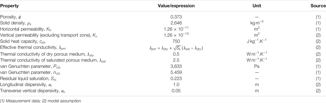
TABLE 1. Porous medium properties used in the numerical model.

The above mass and energy balance equations Eq. 1 (written for three components) and (Eq. 5) would allow us to determine four primary variables. In this study, we chose the following set of primary variables: P_G (gas pressure), P_cap (capillary pressure), X^c (overall molar fraction of the contaminant, Eq. 17) and T (temperature). Such choice of primary variables would imply that phase transition is not accounted for in our model. Instead, the model assumes that the gas phase is always present to at least some minimal saturation $S_G^{\mathrm{m}\mathrm{i}\mathrm{n}}=10^{-4}$ (Yu et al., 2009). Alternatively, completely drying out of the porous medium (i.e. S_G = 1) can be avoided by modification of the capillary pressure model (see Section 3.3).

2.2 Constitutive Relationships

Apart from the four primary variables introduced above, there are ten additional unknowns in Eqs 1–7, i.e., P_L, S_L, S_G, N_L, N_G, $x_L^w$, $x_L^c$, $x_G^w$, $x_G^a$ and $x_G^c$. Since these variables are dependent on the primary variables, they are known as secondary variables. In Eqs 8–17, the constitutive relationships describing such dependency are summarized. Together with the global conservation equations, the necessary closure is formed for the unique solution of the problem.

Eqs 8–10 are the intrinsic constraints of a two-phase and three-component system. Eqs 11, 12 describes the local capillary equilibrium, in which the capillary pressure P_cap is a monotonically decreasing function of the liquid saturation S_L (e.g., van Genuchten model in Eq. 18). Eqs 13, 14 compute the phase molar densities. Specifically, the ideal gas law is assumed for the gas phase, while the molar density of the liquid phase can be approximated as that of the liquid water (as long as the aqueous solubility of the contaminant is small enough). Moreover, Raoult’s Law (Eq. 15) and Henry’s Law (Eq. 16) are applied to describe the equilibrium partitioning of water and organic contaminant between the two fluid phases. For the considered non-isothermal problem, the Henry constant H(T) of the organic contaminant is a temperature-dependent parameter. Additionally the water vapor pressure P_vap is calculated after regulation of capillary effects (Bourgeat et al., 2008). Its detailed expression as a function of P_cap, N_L and T can be found in Sect. S1 of the Supplementary File. Finally, Eq. 17 defines the contaminant overall molar fraction as the weighted mean of its phase-specific molar fractions.

The above set of governing equations was implemented as an extension of the finite-element simulator OpenGeoSys. The implemented model has been validated against several benchmark problems. Since the heat and mass transfer of the original two-phase two-component model was already validated (Huang et al., 2015; Huang, 2017), only the mass transport portion for the third component (organic contaminant) is validated here. To do this, the experimental data of measured gas phase TCE concentration from McCarthy and Johnson (1993) along with the semianalytical solution given by Atteia and Höhener (2010) was compared with model simulation. A very good agreement was obtained for the above comparison, for which more details are documented in Sect. S2 of the Supplementary File.

3 Numerical Model

In this section, the numerical model of a BTES installation operating in a shallow, unconfined aquifer with CHC-contaminated groundwater is described. Here, the model configuration is intentionally kept as simple and concise, since our aim is not to represent realistic field-scale scenarios of BTES application and its interaction with subsurface contamination, but rather to highlight the fundamental mechanisms governing the fate and transport of CHC contaminants in such context.

3.1 Geometry

Figure 1 illustrates the geometrical setup of the numerical model, which represents an unconfined sandy aquifer with dimensions of 59 m × 40 m in x−and z−directions. The groundwater table is located at a depth of 5 m below surface. Currently the model is only two-dimensional (2D) to save computational resources. Due to the 2D setup, the model tends to overestimate the size of the simulated thermal plume (Piga et al., 2017) and thus the volatilization flux of TCE compared with a full 3D model.

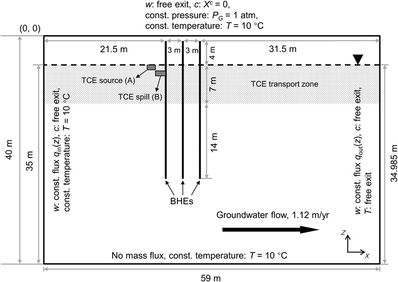
FIGURE 1. 2D setup of the numerical model including geometry and boundary conditions. Dashed line indicates the location of water table.

3.2 Initial and Boundary Conditions

The initial conditions for the gas pressure and capillary pressure are hydrostatic with respect to the groundwater table. Besides, the gas pressure is fixed at 1 atm (101,325 Pa) at the ground surface. Based on the capillary pressure model applied for the sand (Table 1), the initial degree of saturation as a function of depth is depicted in Figure 2A. The regional groundwater flow is assumed from left to right, at a specific discharge of 3.07 × 10³ md⁻¹. This translates to a transport velocity of 3.0 m y⁻¹ given an effective porosity of 0.373 (Table 1). The rationale for the relatively small magnitude of groundwater flow assumed here is to reduce the advective losses of the heat storage while allowing the presence of the TCE plume by groundwater advection and dispersion. For the modeling of groundwater flow in a variably-saturated aquifer, we assigned constant while depth-dependent water fluxes on the left and right boundaries (Figure 2B). Specifically, the boundary water fluxes are scaled by the relative permeabilities at the respective depths. This results in uniform boundary fluxes in the saturated zone and abruptly decreasing ones above the water table.

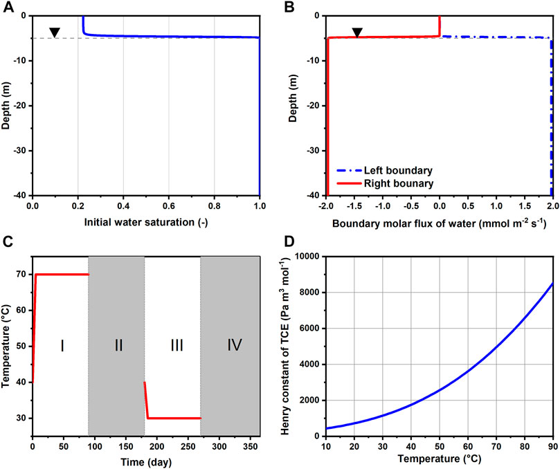
FIGURE 2. (A) Initial water saturation along depth, (B) molar fluxes of water imposed as Neumann boundary conditions, (C) temperature Dirichlet boundary condition imposed for the BHEs annually and (D) change of TCE Henry constant with temperature. Horizontal dashed lines indicate the location of water table.

In this study, we chose TCE as the CHC contaminant of interest. The initial TCE concentration follows a Heaviside step function, i.e. the TCE molar fraction X^c is assumed to be 1 × 10⁻⁵ inside the source/spill location and null over the rest of the domain (Figure 1). Depending on whether the TCE is continuously released from a source (Section 3.4), X^c is either fixed at 1 × 10⁻⁵ within the source location (Box A) or set free. To facilitate TCE emission into the atmosphere, X^c is forced to zero at the top surface for simplicity. The contaminant TCE is set as conservative, with no sorption or biodegradation.

The initial condition for temperature is assumed uniformly at 10 °C across the entire model domain. The identical temperature was also used for Dirichlet boundary conditions on the left, top (assume to be insulated) and bottom boundaries. Seasonal heat storage and extraction is implemented with three BHEs at a 3 m spacing (Figure 1). In reality this could represent a 2D cross-section of a pilot-scale BTES system with 3 × 3 BHEs. The BHEs are modeled by line heat sources reaching a depth of 25 m below ground surface. For simplicity, the topmost 1 m of the BHEs are neglected assuming no heat exchange with the surrounding soil (i.e. perfectly insulated). For the annually repeating charging and discharging of heat, each year (365 days) is divided into four continuous phases of 90 (I), 90 (II), 90 (III), and 95 (IV) days (Figure 2C). Among them, Phase I and III are the heat injection and extraction periods, respectively. During this time, the temperature along the BHEs is assumed constant at either 70 or 30°C except for the initial 5 days of a gradual transition from 40°C. The authors are aware that the fluid temperature inside the BHEs can be very transient in real applications, nevertheless the constant temperature assumed here provides a simple boundary condition for mimicking the cyclic temperature effects of seasonal heat storage. Otherwise, the remainder of the year (Phase II and IV) are standstills of operation, i.e., no temperature boundary conditions are imposed for the BHEs. During heating, water vapor can freely escape from the subsurface by gas-phase advection. Finally, free-exit boundary condition is also applied on the right border for all components as well as heat.

3.3 Parameterization

Table 1 summarizes the porous medium properties assumed for the numerical model. The porosity, bulk density, permeability and water retention characteristics (van Genuchten model parameters) of the porous medium are taken from a set of measurement data from Kiel University (Hailemariam and Wuttke, 2017; Hailemariam and Wuttke, 2020) for a specific type of sand commonly found in Northern German Plain. The remaining properties are assumed based on typical ranges of aquifer material. Here, we assume the permeability of the sand to be anisotropic and use the measured value only for the horizontal component. Meanwhile, the vertical permeability is assumed to be 0.01 times that of the horizontal component except for the “TCE transport zone” (shaded area below the water table in Figure 1). There the vertical permeability is assigned according to scenario specifications (Table 3). Furthermore, the dependency of effective thermal conductivity on the liquid phase saturation is described by the Somerton model (Somerton et al., 1974), i.e., square-root increase. In lack of measurement data, thermal conductivities of dry and water-saturated soil were set to 0.5 and 2.5 W m⁻¹.K⁻¹, respectively. In addition, the capillary pressure and relative permeability functions are given by the van Genuchten (vG) model (van Genuchten, 1980)

where $m_{\mathrm{v}\mathrm{G}}=1-\frac{1}{n_{\mathrm{v}\mathrm{G}}}$ and the effective saturation S_eL is given by

In Eqs 18–20, it is assumed that S_L > S_rL. However, to account for the possible drop of S_L below residual saturation S_rL due to heating of partially-saturated soil, the original capillary pressure curve is modified according to Huang et al. (2015) by linear extrapolation to the segment where S_L⩽S_rL. This leads to an extended vG curve with $P_{cap}^{\mathrm{m}\mathrm{a}\mathrm{x}}=1.46\times 10^8$ Pa at S_L = 0. Likewise, a minimum relative permeability of $k_{rL}^{\mathrm{m}\mathrm{i}\mathrm{n}}=1\times 10^{-8}$ was assumed for the liquid phase. Finally, mass dispersivities of TCE were assumed as α_l = 1 m and α_t = 0.05 m whereas thermal dispersion is neglected in all simulations.

Table 2 lists all relevant properties assigned for the chemical components and fluid phases. Of particular note is the temperature-dependency of certain parameters. Here, the water density is provided as a lookup table from the IF97 data (Kretzschmar and Wagner, 2019), while its viscosity is calculated by the empirical model of Yaws (Yaws, 2014; Beyer et al., 2016). In particular, the temperature-dependent Henry coefficient of TCE is parameterized with the recently published data by Schwardt et al. (Schwardt et al., 2021), with effective temperature ranges up to 90°C (Figure 2D for its increase with temperature). Additionally, all molecular diffusion coefficients are temperature-dependent. The gas phase diffusivities are given by the Fuller’s extrapolation method (Tang et al., 2015) whereas the TCE diffusivity in water is computed through the Arrhenius (exponential) relation.

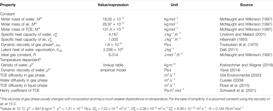
TABLE 2. Component and phase property data.

3.4 Numerical Simulations

In the numerical model, spatial discretization was performed with the standard Galerkin finite element method. Specifically, the 2D domain was discretized into 23,106 quadrilateral/triangular elements and 23,228 nodes with a minimum grid spacing of 5.5 × 4.0 cm in the x− and z− directions. In particular, mesh refinement was performed in the following key locations: 1) near the BHEs in the unsaturated zone, where high gradients of capillary pressure are expected during heat injection; 2) along the vertical direction immediately above the water table, since there will be high gradients of the overall molar fraction X^c and 3) below the water table until a depth of z =−12 m (TCE transport zone), so as to minimize the numerical dispersion associated with TCE transport. A mesh convergence test was conducted, and it was confirmed that further spatial discretization achieves the same simulation result. Meanwhile, temporal discretization follows the implicit Euler scheme. An automatic time-step adjustment is applied based on the number of iterations necessary for the previous time-step. The maximum time-step size was not allowed to exceed 6 days, which fulfills the Courant criteria [i.e., vΔt⩽Δx, Jang and Aral (2006)]. The resulting system of coupled residual equations was linearized with the Newton method and subsequently solved with the BiCGSTAB strategy using ILUT preconditioner.

Table 3 lists the configuration of all simulated scenarios. As aforementioned, the specific scenarios are divided into two categories distinguished by different forms of contamination, i.e. constant source (continuous plume, Group A) and instantaneous spill (discontinuous plume, Group B). In each group, a baseline scenario (A0 and B0) without BTES operation, i.e. under isothermal condition, is simulated. Among the BTES scenarios, A1 and B1 were simulated without the effect of buoyant flow. This was done by reducing the transport zone vertical permeabilities of these scenarios to 1/100th of the rest of the domain. Alternatively, the vertical permeability inside the transport zone was not reassigned for other scenarios. The simulated time period was 5 years for all scenarios.

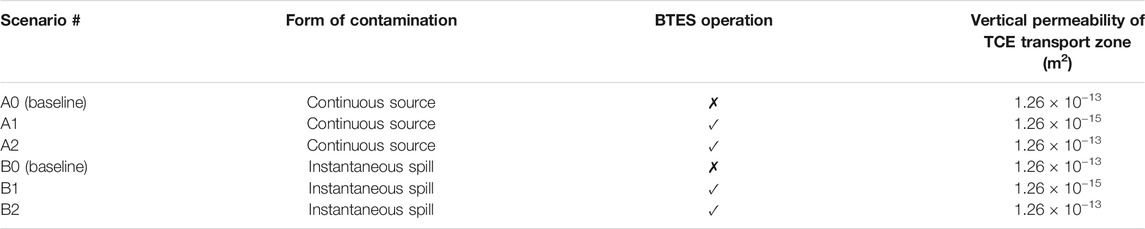
TABLE 3. Description of simulated scenarios.

4 Results

4.1 TCE Transport Without Thermal Energy Storage

Figures 3A,B depicts the distribution of TCE molar fraction in the liquid and gas phases after 5 years in Scenario A0. Here, logarithmic scale is used for the TCE molar fractions in order to illustrate both saturated and unsaturated zones (same for below). In Figure 3A, a groundwater plume of dissolved TCE has formed in the downgradient of the source due to advective-dispersive transport in the liquid phase. Besides, both aqueous and gas phase TCE plumes can also be observed in the unsaturated zone. Particularly for the liquid phase, TCE molar fraction appears to be significantly smaller above the water table than below. A further examination of the depth profiles (Figure 3C) reveals that both liquid and gas phase molar fractions of TCE decreased by an order of magnitude at a distance of approximately 0.4 m above the water table. Such abrupt changes are caused by the depth-dependent transport mechanisms of TCE across the capillary fringe. Here, we briefly describe the underlying physical processes as a more detailed semi-quantitative analysis is presented in Sect. S3 of the Supplementary File. As observed by McCarthy and Johnson (1993), vertical mass exchange between saturated and unsaturated zones is controlled by aqueous phase diffusion. This can be related to the fact that TCE diffusivity in the liquid phase is nearly four orders of magnitude smaller than that in the gas phase (Table 2). In this work, the effect of hydrodynamic dispersion is considered in addition to molecular diffusion in the liquid phase. Despite such difference, the overall diffusive force in the saturated zone is still one to two orders of magnitude less than that in the unsaturated zone away from the water table. Therefore, the McCarthy and Johnson hypothesis can be extended by stating that, even with the additional contribution from hydrodynamic dispersion, vertical mass fluxes from the groundwater will be relatively small due to limitations in aqueous phase transport. As a consequence, natural attenuation of the contaminant plume through volatilization and subsequent release into the atmosphere is a rather slow process. The above conclusion is expected to be valid in most subsurface conditions since the vertical dispersivity of 0.05 m assumed in this study is already a relatively high value in natural aquifers (Rotaru et al., 2014).

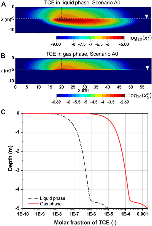
FIGURE 3. (A) Liquid, (B) gas phase molar fraction of TCE after 5 years for Scenario A0 and (C) depth profiles in the unsaturated zone at x = 20 m [dash-dotted line in (A) and (B)].

4.2 Effect of Temperature-enhanced Volatilization on TCE Transport

Figure 4 depicts the distribution of temperature and liquid saturation after 5 years of BTES operation for Scenario A1. The temperature and saturation contours from other BTES scenarios displayed very similar patterns and are thus not shown. Due to the unbalanced heat injection and extraction loads, a thermal plume has evolved downgradient of the BHEs, with the highest temperature reaching 35.4°C (Figure 4A). Meanwhile, changes in the liquid saturation are mostly found directly above the BHEs in the unsaturated zone. Specifically, a recondensation zone with liquid saturation up to 0.3 has developed between the BHEs and the top boundary. The increased liquid saturation in turn leads to locally higher TCE molar fractions in both liquid and gas phases. Nevertheless, TCE molar fractions are already very low near the top boundary and thus the influence of saturation changes on the mass transport of TCE is expected to be negligible in the simulated scenarios.

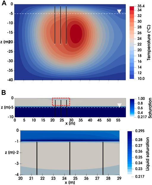
FIGURE 4. Distribution of (A) temperature and (B) liquid saturation after 5 years of BTES operation for Scenario A1.

In Figure 5, the simulated total TCE concentration after 5 years is illustrated for various scenarios. Here, we only focus on the comparison between baseline scenarios (A0 and B0) and BTES scenarios without buoyant flow (A1 and B1). In general, the effect of BTES operation on the development of TCE plume seems to be limited for both Scenario A1 and B1. Although the TCE concentration in the unsaturated zone has diminished to some extent compared to the baseline, only a slight mitigation of the TCE plume was found in the saturated zone.

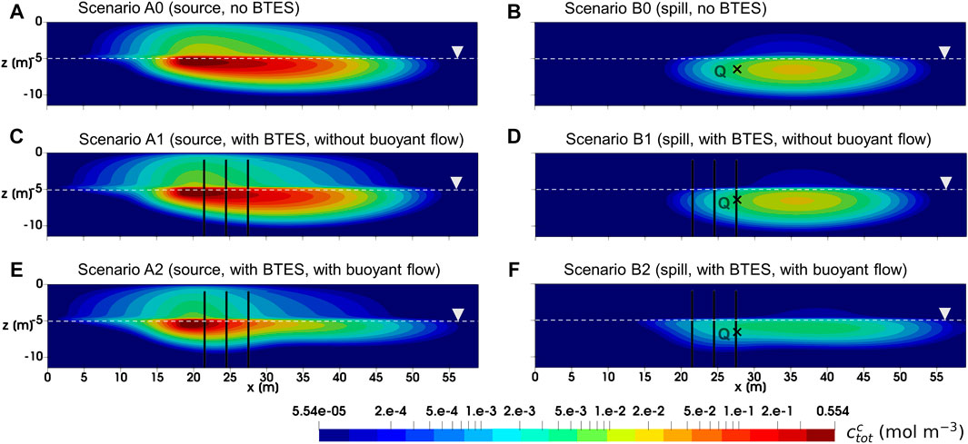
FIGURE 5. Total TCE concentration at 5 years for all simulated scenarios. Note that the concentration contours are presented in logarithmic scale. Black cross represents the location of observation point Q.

For a quantitative evaluation of TCE fate and transport, mass balance calculations were performed and the results are shown in Figures 6, 7 for Group A and B scenarios respectively. Here, only the “free” TCE which is outside the source is considered for the liquid phase. In general, a very good accuracy was achieved for all conducted simulations, as mass balance errors accumulated up to 5 years and at every time step were less than 2.8 and 0.08%, respectively. For the Group A scenarios assuming constant source, a slightly faster release of TCE from the source is observed for Scenario A1 comparing to the baseline, as shown in Figure 6A. Such behavior is attributed to the decrease of water viscosity with temperature, leading to increased flow velocities and thus water fluxes (“flow focusing”) within the heated source (Beyer et al., 2016). In Figure 6B where the cumulative TCE volatilization is plotted, BTES-induced temperature increase (Scenario A1) led to a 39% higher TCE mass transfer to the gas phase at the end of simulation. In particular, the increased amount of volatilized TCE (0.73 mol difference after 5 years) was able to offset the negative impact of increased TCE emission from source (0.44 mol difference after 5 years) resulting from BTES operation. As a result, a 0.29 mol decrease in the residual liquid phase TCE is obtained for Scenario A1 compared to baseline at the end of simulation (Figure 6C). In Figure 6D, the gas phase TCE of Scenario A1 shows overall higher status compared to Scenario A0, due to its higher volatilization. This is particularly evident at the beginning of heat injection phases where a sharp rise of the gas phase TCE can be noticed. Nevertheless, the above difference between Scenario A1 and A0 is diminishing at the end of each year. In Figures 7B–D, a similar pattern of TCE mass transfer can be observed for the instantaneous spill scenarios B0 and B1. Here, we note that an appreciable TCE volatilization only occurred after the first year in both scenarios (see Figure 7B). This is due to the fact the initial spill is located 1 m below the water table and that vertical transport of TCE by groundwater dispersion is rather slow.

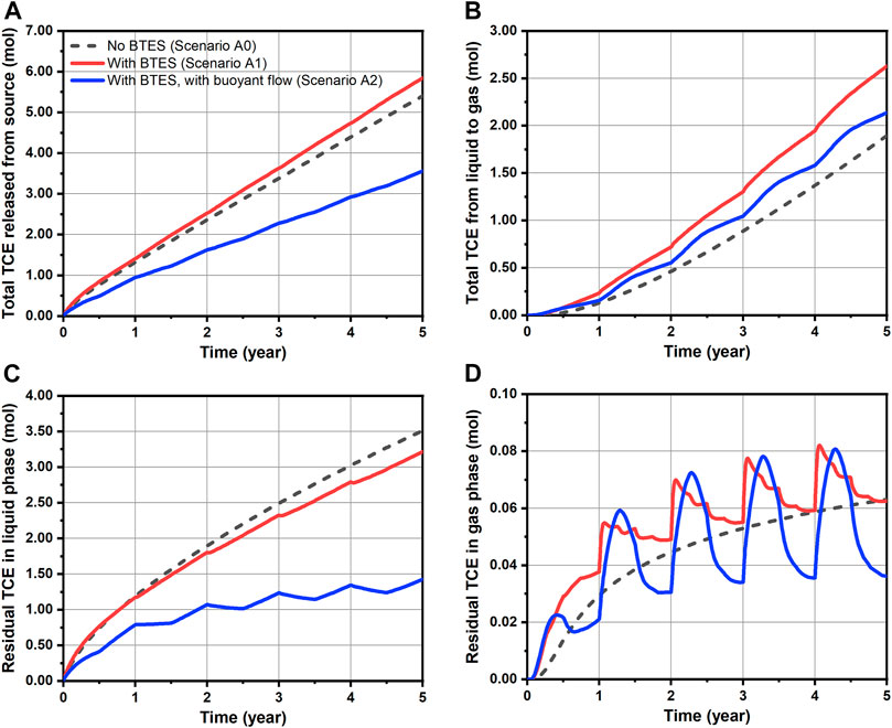
FIGURE 6. Transport dynamics of TCE for simulated scenarios assuming constant source: (A) released amount from source, (B) total amount transferred from liquid to gas phase, (C) residual amount of mobile TCE in the liquid phase and (D) residual amount of TCE in the gas phase.

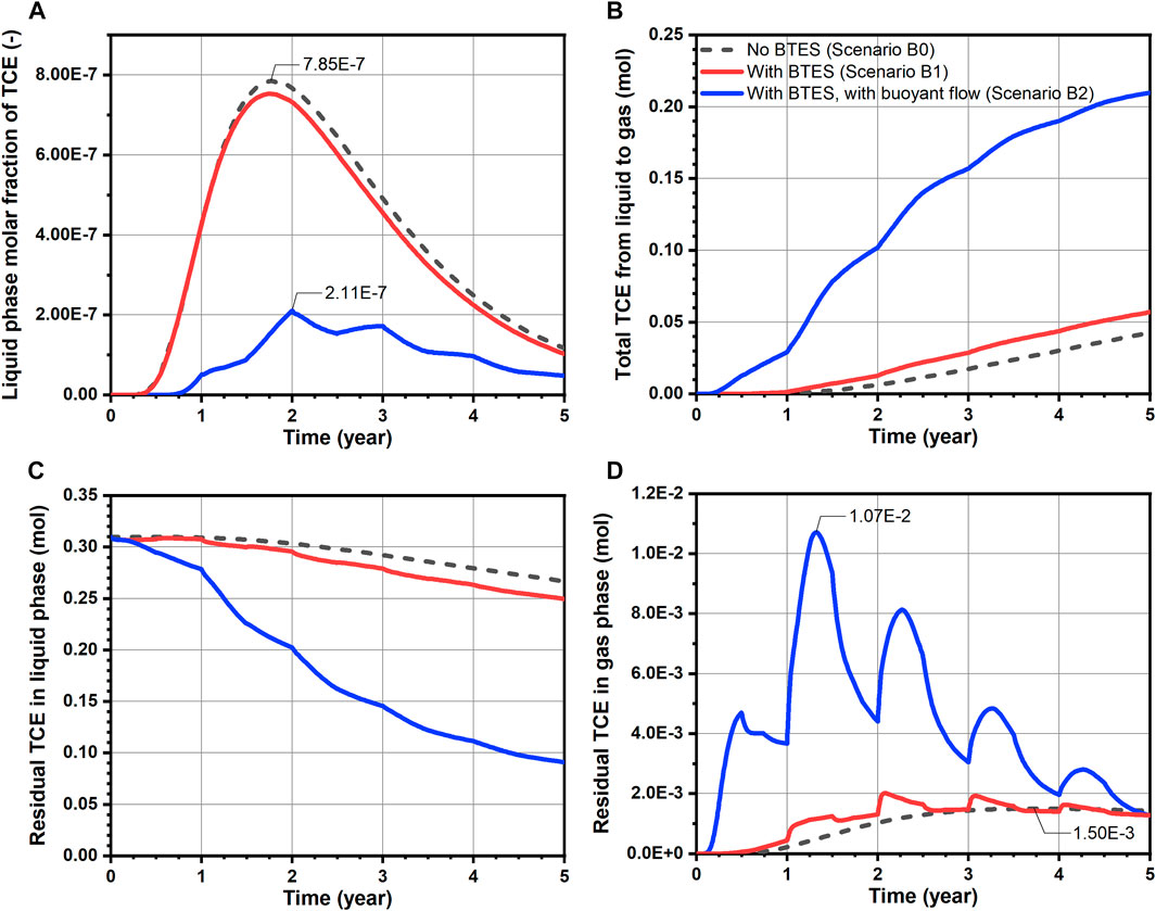
FIGURE 7. Transport dynamics of TCE for simulated scenarios assuming instantaneous spill: (A) breakthrough curves of TCE molar fraction at observation point Q (Figure 5B, (B) total amount transferred from liquid to gas phase, (C) residual amount of TCE in the liquid phase and (D) residual amount of TCE in the gas phase.

Table 4 summarizes the reduction of total TCE mass for all simulations. Here, the residual amount of TCE includes contribution from both liquid (only “free” portion) and gas phases. As perceived from the foregoing analysis, the effect of BTES-enhanced attenuation of TCE are indeed quite limited in Scenario A1 and B1. The decrease in the residual TCE amount compared to the baseline are less than 10% in both scenarios. Although a moderate reduction rate of 44% is obtained for Scenario A1, such number is mainly attributed to the favorable location of the source (i.e. directly beneath the water table), rather than the additional benefit from BTES. This can be supported by the relatively small improvement of Scenario A1’s reduction rate compared to Scenario A0s. Hence, we conclude that the limiting factor for the transfer of dissolved TCE to the unsaturated zone is still the slow dispersive transport in the aqueous phase. As a consequence, temperature-enhanced volatilization can only result in a superficial reduction of TCE mass below the water table, whereas the deeper part of the plume is largely excluded from being remediated.

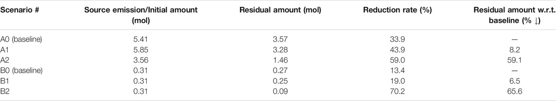
TABLE 4. Summary of TCE reduction after 5 years for all simulated scenarios.

4.3 Effect of Buoyant Flow on TCE Transport

In practical BTES applications, buoyant flow may be induced in medium to high permeability aquifers due to the temperature-dependent water density (Catolico et al., 2016; Boockmeyer, 2020). Since Scenario A2 and B2 are distinguished by a 100 times larger vertical permeability of the transport zone, buoyant flow is more likely to develop in these scenarios and in turn affect the mass transport of TCE.

Figures 8A,B illustrate the magnitude of vertical Darcy velocity after 1,550 days of BTES operation (i.e., after the fifth heat injection phase) for Scenario A1/B1 and Scenario A2/B2, respectively. Here, the liquid phase velocity field is identical for different contamination scenarios with the same vertical permeability, as the TCE concentration is too low to induce any changes in the liquid flow regime. In contrast to Scenario A1/B1 with virtually no buoyant flow, a moderate buoyant flow is found for Scenario A2/B2 in the vicinity of the BHEs, as evidenced by the considerably higher vertical velocities there in Figure 8B. In particular, the simulated maximum Darcy velocity in the z direction for Scenario A2/B2 equals to 0.6 m y⁻¹, which is in the same order of magnitude as the undisturbed groundwater flow velocity. This leads to the groundwater being directed upwards when passing through the heated zone, as marked by the arrows indicating flow direction in Figure 8B. As the heated water rises to the water table, it tends to spread in the left and right directions due to the much larger horizontal permeability. As a result, the horizontal flow velocity below the water table is also influenced by the buoyant flow. For example, the simulated horizontal velocity profile for Scenario A2/B2 at z = −5.5 m in Figure 8C shows a strong retardation in the upgradient, yet acceleration in the downgradient of the BHEs. Furthermore, a circular flow regime can even be recognized between x = 15 and 20 m in Figure 8B. The above flow pattern as a whole can be described as “mixed flow” (Haajizadeh and Tien, 1984), due to the fact that both buoyant flow and groundwater advection are occurring and interacting with each other.

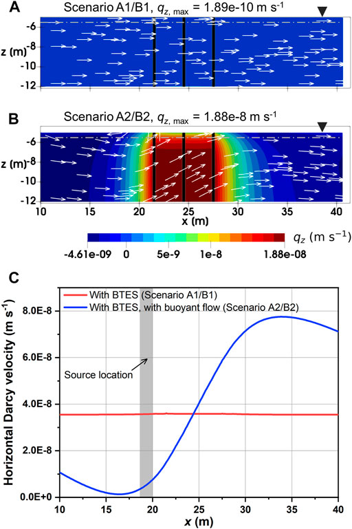
FIGURE 8. Darcy velocity in the transport zone after 1,550 days: (A) magnitude of vertical velocity for Scenario A1/B1, (B) magnitude of vertical velocity for Scenario A2/B2 and (C) horizontal Darcy velocity profile at z = − 5.5 m [dash-dotted line in (A) and (B)]. White arrows in (A) and (B) indicate the liquid phase velocity field (not to scale).

The effect of buoyant flow on the development of TCE plume can be visualized in Figures 5E,F. In Scenario A2 where a constant source was assumed, the TCE concentration plot shows essentially lower concentrations in the downgradient direction along with a thinner plume below the water table. Besides, it is noted that the TCE concentration in the unsaturated zone is also reduced. On the other hand, a likewise reduction of TCE concentration is also predicted for Scenario B2 assuming initial spill. In particular, the TCE plume appears to be more “stretched out” horizontally due to the expanded advective velocity as well as hydrodynamic dispersion in the horizontal direction. To further illustrate the effect of buoyant flow on the reduction of TCE concentration, the breakthrough curves of (liquid phase) TCE molar fraction observed at 6.14 m downgradient of the spill location (point Q in Figure 5) are illustrated in Figure 7A. With respect to the peak molar fraction, Scenario B2 reported a 73.1% decline compared to Scenario B0, indicating a significant reduction. Furthermore, a comparably delayed arrival of the bulk mass is observed in Scenario B2, due to the mostly reduced horizontal Darcy velocity upgradient of the observation point.

Temporal TCE mass transfer under the influence of buoyant flow is illustrated with the blue curves in Figures 6, 7. For the continuous source scenario (A2), buoyant flow is recognized to contribute to the overall reduction of TCE through two distinct mechanisms. 1) In Figure 6A, the TCE release curve of Scenario A2 is much flatter when compared to Scenario A0 and A1. This is due to the inhibited horizontal flow around the source in Scenario A2 (Figure 8C). As a result, up to 34% less TCE is released from the source after 5 years in Scenario A2 compared to the baseline (A0). 2) In Figure 6B, despite the less amount of TCE emitted from the source, a higher amount of TCE is volatilized into the gas phase in Scenario A2 than A0 (although still lower than Scenario A1). This is attributed to the induced buoyant flow in Scenario A2 which enhanced the mass transfer of aqueous TCE to the unsaturated zone by advection. Consequently, an enlarged proportion of the released TCE is volatilized in Scenario A2 (60.0%) compared to Scenario A0 (35.1%) and A1 (45.3%). The above two mechanisms led to a notable mitigation in the growth of residual TCE in both liquid and gas phases, as shown in Figures 6C,D. Compared to Scenario A1, the residual TCE curves of Scenario A2 exhibit larger fluctuations since the percentage of volatilized TCE is higher. Finally, we see in Table 4 that the buoyancy effect of Scenario A2 resulted in a nearly 60% decline of the total residual TCE in comparison to Scenario A0, showing a remarkable improvement from Scenario A1 where only temperature-enhanced volatilization is considered. Again, such improvement is the combined outcome of reduced emission from the source and the stimulated mass transfer to the unsaturated zone.

In Figures 7B–D, a considerable improvement in TCE volatilization and reduction is also predicted for Scenario B2. Since there is no release of the contaminant from the source, the dominant mechanism to facilitate the TCE mass transfer here is obviously the heating-induced buoyant flow. This can be witnessed from the following characteristics of Scenario B2’s volatilization curve in Figure 7B. First, an earlier TCE volatilization is observed in Scenario B2. Instead of after 1 year in scenarios without buoyant flow, the volatilized TCE is already appreciable after 0.25 years in Scenario B2. Such difference is caused by the buoyant flow driving the TCE towards the water table during the first heat injection phase. Secondly, the total volatilized TCE shows a strong increasing trend during the second and third years, whereas the growth becomes much less intense thereafter. Despite the fact that the residual TCE mass is diminishing, another important reason is that the majority of TCE at highest concentrations has escaped from the buoyancy-influenced zone (Figure 8B), which also tends to slow down the volatilization rate. Nevertheless, the total volatilized TCE in Scenario B2 reaches 0.21 mol after 5 years, being almost five times that of the baseline (B0). As a direct consequence of volatilization, the evolution of residual aqueous TCE in Figure 7C for the spill scenarios is practically a mirrored image of Figure 7B, indicating a major reduction in the dissolved TCE mass due to buoyant flow. Finally, in Figure 7D, although the gas phase TCE of Scenario B2 showed strong oscillations due to the highest volatilization rate, its final amount after 5 years is indeed similar to the baseline. Together with the flattening volatilization curve (Figure 7B), remediation is almost completed at this time. As a consequence of the enhanced TCE transport due to buoyant flow, the residual TCE mass in the domain is less than 0.1 mol in Scenario B2, showing a 66% reduction from the baseline (Table 4). Besides, the highest TCE reduction rate of over 70% is achieved in Scenario B2 among all simulated scenarios. In conclusion, in cases where the contaminant plume is well-characterized and discontinuous, a substantially enhanced volatilization can be achieved by taking advantage of the buoyant flow effect during BTES operation.

5 Discussion

5.1 Effect of Buoyant Flow on Heat Storage Efficiency

The simulation results of Scenario A2 and B2 suggest that high permeability could be a positive factor by promoting thermally-induced buoyant flow and contributing to an increased volatilization of the contaminant. However, high permeability may at the same time be a negative factor for the heat storage efficiency (i.e., ratio of extracted vs. injected heat in an operating year) of BTES applications (Catolico et al., 2016; Djotsa Nguimeya Ngninjio et al., 2021). Catolico et al. (2016) simulated the heat storage efficiencies at varying permeabilities in an unconfined aquifer without groundwater flow. Their simulation results showed that a decrease in storage efficiency occurs only at permeability values greater than 1.5 × 10⁻¹² m². In our work though, the scenario setting is a bit more complicated since the permeability is assumed to be anisotropic and that a moderate groundwater flow exists. By comparing the simulated temperature distributions at the end of each heat injection and extraction period, the maximum difference between Scenario A1/B1 and A2/B2 is less than 1 K, which implies that the temperature distribution is not greatly affected by buoyant flow. However, to precisely determine whether the enhanced contaminant reduction at higher permeabilities is associated with the loss of heat storage efficiency, a detailed 3D heat transport analysis would be necessary which is beyond the scope of this study.

5.2 Implications for Combining BTES and Groundwater Remediation

In this study, we demonstrated the potential compatibility of BTES with contaminated aquifers to achieve an enhanced remediation of CHC contaminants. An important finding is that the buoyant flow induced by heat storage plays an essential role in the improvement of TCE volatilization. As our basic hypothesis, vertical mass transfer of the dissolved contaminant is limited by the slow aqueous phase dispersion. This implies that the difficulty of removing the contaminant increases dramatically when it sinks deeper into the saturated zone (Ni et al., 2015a; Janfada et al., 2020). Thus, in order to achieve significantly enhanced in-situ volatilization, it is important to overcome the above limitations in aqueous phase transport. Here, such principle is primarily manifested by the buoyant flow resulted from conductive heating, which enables an accelerated TCE migration to the unsaturated zone. Alternatively, a separate gas phase can be injected to facilitate the partitioning and mobilization of the contaminant, e.g. in steam injection (Hiester et al., 2013) and air sparging. Furthermore, it is worth noting that the modeled BTES system here is quite small in size. In practical BTES applications, typically large arrays of borehole are arranged in compact shapes (e.g., cylindrical) in order to increase the heat storage volume while minimizing heat losses. Therefore, real heat storage systems are expected to attain higher remediation capacities than demonstrated in this study. Considering a typical BTES lifetime of 25-30 years, complete removal of CHC plumes may appear as a feasible and attractive remediation goal even within the first few years of operation.

Besides the benefit of enhanced contaminant attenuation which occurs mainly in the saturated zone, a relocation of the volatilized contaminant into the unsaturated zone is also predicted by the numerical model. Here, the main concern from an environmental perspective is the potentially elevated contaminant concentration in the gas phase which may give rise to vapor intrusion and adversely impact the indoor air quality (Wang et al., 2012). Regarding this concern, our simulation results yield different outcomes depending on the time scale considered. In Figures 6D, 7D, the gas phase TCE content of Scenario A1, A2 and B2 showed relatively large temporal fluctuations with respect to the baseline curve. Especially in Scenario B2, the maximum amount of gas phase TCE reaches 0.011 mol, which is more than seven times higher than that of the baseline (1.50 × 10⁻³ mol). Therefore, in short time scales (e.g., months to a few years), the significantly raised contaminant vapor concentration could possibly lead to indoor air regulations being exceeded when residential dwellings are nearby. Nevertheless, it is also observed that the gas phase contaminant retains strong “resilience” in response to subsurface temperature fluctuations—after the sharp increase due to heat injection, it was able to recover to a much lower extent at the end of each year. Furthermore, for all scenarios with BTES operation, the gas phase TCE at 5 years is either lower than or at the same level of the baseline. In other words, no significant TCE accumulation in the soil gas is predicted over the longer time scale. Such advantage is mainly attributed to the rapid diffusive transport in the gas phase, thus allowing the TCE vapor to be effectively released to the atmosphere under the high concentration gradients. Since the risk of vapor intrusion cannot be completely ruled out, long-term monitoring of the contaminant vapor concentration in the subsurface is advised to mitigate the above negative impacts of BTES operation. To fully eliminate the risk of vapor intrusion, soil vapor extraction (Baker et al., 2016) can be integrated to remove the contaminated soil gas.

5.3 Model Limitations

Although the investigated scenarios and process interactions are already quite complex, the applied numerical model still neglects several processes that may become relevant in the context of thermal energy storage in contaminated subsurface. Owing to the assumption of a two-phase (water-air) system, the model does not account for the existence of CHC contaminants as pure NAPL phase in the subsurface. When the contaminant source is present as residual NAPL phase, temperature variations may have additional impacts on NAPL solubility (Popp et al., 2016; Koproch et al., 2019), mobility (Philippe et al., 2020), etc. These effects may lead to further release and transport of the contaminant. Otherwise, when NAPL phase is present in the unsaturated zone, even in traces, the volatilization flux will be considerably higher (Ostendorf et al., 2000). Hence, the presented model is most favorably applied in areas downgradient of identified source zones, where the contaminant is already fully dissolved in the aqueous phase.

Another limitation of the numerical model is that phase transition is so far not considered. As a result of heat storage in saturated porous medium, gas phase may develop and accumulate in case of large temperature elevations at shallow groundwater depths. The formation of a gas phase can have multiple influences on heat storage and aquifer contamination, as detailed in the work of Lüders et al. (2016). One potential outcome is that the dissolved contaminant can be transported further when gas bubbles are mobilized. Since the formation of gas phase is strongly dependent on the composition of dissolved gases in groundwater (Lüders et al., 2016), simulation of such process would in general require at least four components in the model. Last but not least, many other physical and chemical processes such as sorption and biodegradation also respond actively to temperature changes. Although the abovementioned processes are important, they are beyond the scope of this study and will be investigated in future research.

6 Conclusion

This study aimed at understanding the effects of high-temperature BTES on the fate and transport of CHC contaminants by simulating the coupled fluid flow, heat and mass transport in a variably-saturated aquifer using OpenGeoSys software. The thermal impacts on the subsurface resulting from seasonal heat storage was examined in a contaminant transport context by means of two-phase flow modeling using temperature-dependent parameters. Application of the numerical model is demonstrated for a series of scenarios of BTES operation in a shallow unconfined aquifer contaminated by TCE. The main findings of this study are hereby summarized:

1) The key mechanism limiting the transfer of the contaminant from the groundwater to the unsaturated zone is the dispersive transport process in the liquid phase.

2) Temperature increase in the subsurface can lead to an enhanced volatilization of the contaminant in groundwater. However, temperature effect alone is only able to remediate the uppermost part of the saturated zone whereas the deeper contaminated regions are practically unaffected.

3) At higher soil permeabilities, buoyant flow may be induced due to heating of the groundwater. This can change the flow dynamics and result in a significant improvement of contaminant removal.

For a constant source: Buoyant flow reduces the contaminant emission from source while at the same time drives the contaminant plume towards the water table. The combined effect led to a nearly 60% decline in residual TCE mass after 5 years of BTES operation.

For an instantaneous spill: Buoyant flow accelerates the volatilization process and increases the overall reduction of TCE from 19% to over 70%.

4) Contaminant concentration in the soil gas showed large temporal fluctuations in response to seasonal heat storage. In spite of this, seasonal heat storage was not found to further increase the soil gas content of the contaminant in the long-term.

Considering the relatively small size of the modeled BTES system, the potential of BTES in assisting the in-situ volatilization of CHC contaminants in groundwater looks promising. As a consequence, the combination of underground heat storage with the remediation of contaminated aquifers offers an environmentally and energetically sustainable way to foster the redevelopment of contaminated urban areas. Despite the general benefits predicted, it is important to note that many other factors for physical, chemical, biological, and geological conditions can impact the contaminant transport during heat storage in the shallow subsurface. Thus, future work should include a more comprehensive and site-specific assessment of the temperature effects to ensure that the benefits anticipated for the combination of BTES and enhanced volatilization outweigh the risk of contaminant spreading, especially when subsurface heat storage facilities are practiced near NAPL contaminated sites.

Data Availability Statement

The original contributions presented in the study are included in the article/Supplementary Material, further inquiries can be directed to the corresponding authors.

Author Contributions

BM: Methodology, Software, Validation, Formal analysis, Writing—Original Draft, Visualization. YY: Methodology, Investigation, Writing—Review and Editing. YH: Conceptualization, Methodology, Software, Writing—Review and Editing. OK: Writing—Review and Editing, Supervision, Project administration, Funding acquisition. HS: Conceptualization, Methodology, Software, Writing—Review and Editing, Visualization, Supervision.

Funding

This work was financially supported by the National Natural Science Foundation of China (Grant Number 41902311). This work was also supported by the German Federal Ministry for Economic Affairs and Energy (BMWi) for the “ANGUS II” project (Grant Number 03ET6122B).

Conflict of Interest

The authors declare that the research was conducted in the absence of any commercial or financial relationships that could be construed as a potential conflict of interest.

Publisher’s Note

All claims expressed in this article are solely those of the authors and do not necessarily represent those of their affiliated organizations, or those of the publisher, the editors and the reviewers. Any product that may be evaluated in this article, or claim that may be made by its manufacturer, is not guaranteed or endorsed by the publisher.

Acknowledgments

We would like to thank Christof Beyer (Kiel University) and Wenqing Wang (UFZ) for the fruitful discussions and their insightful comments. BM would also like to acknowledge the financial support from the China Scholarship Council (CSC) for his PhD study in Germany.

Supplementary Material

The Supplementary Material for this article can be found online at: https://www.frontiersin.org/articles/10.3389/feart.2021.790315/full#supplementary-material

References

Glossary

c_p Specific heat capacity (J kg⁻¹.K⁻¹)

$D_{\alpha }^k$ Diffusion coefficient of component k in free phase α (m².s⁻¹)

F^k source or sink term of component k (mol m⁻³.s⁻¹)

g gravitational acceleration (m s⁻²)

H Henry’s law constant (Pa m³.mol⁻¹)

h specific enthalpy (J kg⁻¹) horizontal

h_Δe latent heat of vaporization of water (J kg⁻¹)

I identity matrix

${\mathit{J}}_{\alpha }^k$ diffusive flux of component k in phase α (m s⁻¹)

K intrinsic permeability tensor (m²)

k any of the three chemical components

k_rα relative permeability of phase α (-)

M^k molar mass of component k (kg mol⁻¹)

N_α molar density of phase α (mol m⁻³)

P_α pressure in phase α (Pa)

P_cap capillary pressure (Pa)

P_vap vapor pressure (Pa)

q_α Darcy velocity of phase α (m s⁻¹)

Q_T heat source or sink term (W m⁻³)

S_α saturation of phase α (-)

S_eL effective liquid saturation (-)

S_rL residual liquid saturation (-)

T temperature (K) transpose

u specific internal energy (J kg⁻¹)

X^k overall molar fraction of component k (-)

$x_{\alpha }^k$ molar fraction of component k in phase α (-)

Greek Letters

α either of the two fluid phases

λ_pm effective thermal conductivity of the porous medium (W m⁻¹.K⁻¹)

μ_α dynamic viscosity of phase α (Pa s)

ϕ porosity (-)

ρ mass density (kg m⁻³)

Operators

div divergence operator

V‐ gradient operator

Superscripts

a air

c organic contaminant

T temperature (K) transpose

w water

Subscripts

G gas phase

h specific enthalpy (J kg⁻¹) horizontal

L liquid phase

l longitudinal

s soil grain

v vertical

References

Atteia, O., and Höhener, P. (2010). Semianalytical Model Predicting Transfer of Volatile Pollutants from Groundwater to the Soil Surface. Environ. Sci. Technol. 44, 6228–6232. doi:10.1021/es903477f
Baker, R. S., Nielsen, S. G., Heron, G., and Ploug, N. (2016). How Effective Is thermal Remediation of DNAPL Source Zones in Reducing Groundwater Concentrations? Groundwater Monit. R. 36, 38–53. doi:10.1111/gwmr.12149
Beyer, C., Popp, S., and Bauer, S. (2016). Simulation of Temperature Effects on Groundwater Flow, Contaminant Dissolution, Transport and Biodegradation Due to Shallow Geothermal Use. Environ. Earth Sci. 75. doi:10.1007/s12665-016-5976-8
Boockmeyer, A. (2020). Numerical Simulation of Borehole thermal Energy Storage in the Geological Subsurface. Ph.D. thesis. Kiel University.
Bourgeat, A., Jurak, M., and Smaï, F. (2008). Two-phase, Partially Miscible Flow and Transport Modeling in Porous media; Application to Gas Migration in a Nuclear Waste Repository. Comput. Geosci. 13, 29–42. doi:10.1007/s10596-008-9102-1
Casasso, A., and Sethi, R. (2019). Groundwater-Related Issues of Ground Source Heat Pump (GSHP) Systems: Assessment, Good Practices and Proposals from the European Experience. Water 11, 1573. doi:10.3390/w11081573
Catolico, N., Ge, S., and McCartney, J. S. (2016). Numerical Modeling of a Soil‐Borehole Thermal Energy Storage System. Vadose zone j. 15, 1–17. doi:10.2136/vzj2015.05.0078
Class, H., and Helmig, R. (2002). Numerical Simulation of Non-isothermal Multiphase Multicomponent Processes in Porous media. Adv. Water Resour. 25, 551–564. doi:10.1016/s0309-1708(02)00015-5
Cussler, E. L. (2009). Diffusion: Mass Transfer in Fluid Systems. Cambridgeshire: Cambridge University Press.
Datt, P. (2011). Latent Heat of Vaporization/Condensation. Dordrecht: Springer Netherlands, 703. doi:10.1007/978-90-481-2642-2_327
Djotsa Nguimeya Ngninjio, V., Bo, W., Beyer, C., and Bauer, S. (2021). “Experimental and Numerical Investigation of thermal Convection in a Water Saturated Porous Medium Induced by Heat Exchangers in High Temperature Borehole thermal Energy Storage,” in EGU General Assembly Conference Abstracts, EGU21–8071.
Elhashmi, R., Hallinan, K. P., and Chiasson, A. D. (2020). Low-energy Opportunity for Multi-Family Residences: A Review and Simulation-Based Study of a Solar Borehole thermal Energy Storage System. Energy 204, 117870. doi:10.1016/j.energy.2020.117870
Fleuchaus, P., Godschalk, B., Stober, I., and Blum, P. (2018). Worldwide Application of Aquifer thermal Energy Storage - A Review. Renew. Sust. Energ. Rev. 94, 861–876. doi:10.1016/j.rser.2018.06.057
Grandel, S., and Dahmke, A. (2008). “Natürliche Schadstoffminderung bei LCKW-kontaminierten Standorten Methoden, Empfehlungen und Hinweise zur Untersuchung und Beurteilung,” in Christian-Albrechts-Universität zu Kiel.
GSI Environmental (2020). Gsi Chemical Database. Available at: https://www.gsi-net.com/en/publications/gsi-chemical-database/single/547-CAS-79016.html (Accessed May 14, 2021).
Haajizadeh, M., and Tien, C. L. (1984). Combined Natural and Forced Convection in a Horizontal Porous Channel. Int. J. Heat Mass Transfer 27, 799–813. doi:10.1016/0017-9310(84)90001-2
Hailemariam, H., and Wuttke, F. (2020). Cyclic Mechanical Behavior of Two sandy Soils Used as Heat Storage media. Energies 13, 3835. doi:10.3390/en13153835
Hailemariam, H., and Wuttke, F. (2017). Temperature Dependency of the thermal Conductivity of Porous Heat Storage media. Heat Mass. Transfer 54, 1031–1051. doi:10.1007/s00231-017-2204-3
Heat Roadmap Europe (2017). Heating and Cooling Facts and Figures: The Transformation towards a Low-Carbon Heating & Cooling Sector. [Online], Available from: https://www.isi.fraunhofer.de/content/dam/isi/dokumente/cce/2017/29882_Brochure_Heating-and-Cooling_web.pdf (Accessed September 30, 2021).
Hiester, U., Müller, M., Koschitzky, H., Trötschler, O., Roland, U., Holzer, F., et al. (2013). Guidelines: In Situ thermal Treatment (ISTT) for Source Zone Remediation of Soil and Groundwater. Helmholtz Centre for Environmental Research.
Hilsenrath, J. (1955). Tables of thermal Properties of Gases: Comprising Tables of Thermodynamic and Transport Properties of Air, Argon, Carbon Dioxide, Carbon Monoxide, Hydrogen, Nitrogen, Oxygen, and Steam. Washington D.C.: US Department of Commerce, National Bureau of Standards.
Huang, Y. (2017). Heat Pipe Problem. Available at: https://www.opengeosys.org/docs/benchmarks/thermal-two-phase-flow/heat-pipe/(Accessed September 28, 2021).
Huang, Y., Kolditz, O., and Shao, H. (2015). Extending the Persistent Primary Variable Algorithm to Simulate Non-isothermal Two-phase Two-Component Flow with Phase Change Phenomena. Geotherm Energy 3. doi:10.1186/s40517-015-0030-8
Huang, Y., Shao, H., Wieland, E., Kolditz, O., and Kosakowski, G. (2021). Two-phase Transport in a Cemented Waste Package Considering Spatio-Temporal Evolution of Chemical Conditions. Npj Mater. Degrad. 5. doi:10.1038/s41529-021-00150-z
Imhoff, P. T., Frizzell, A., and Miller, C. T. (1997). Evaluation of thermal Effects on the Dissolution of a Nonaqueous Phase Liquid in Porous media. Environ. Sci. Technol. 31, 1615–1622. doi:10.1021/es960292x
Janfada, T. S., Class, H., Kasiri, N., and Dehghani, M. R. (2020). Comparative Experimental Study on Heat-Up Efficiencies during Injection of Superheated and Saturated Steam into Unsaturated Soil. Int. J. Heat Mass Transfer 158, 119235. doi:10.1016/j.ijheatmasstransfer.2019.119235
Jang, W., and Aral, M. M. (2006). Density-driven Transport of Volatile Organic Compounds and its Impact on Contaminated Groundwater Plume Evolution. Transp Porous Med. 67, 353–374. doi:10.1007/s11242-006-9029-8
Kolditz, O., Bauer, S., Bilke, L., Böttcher, N., Delfs, J. O., Fischer, T., et al. (2012). OpenGeoSys: an Open-Source Initiative for Numerical Simulation of Thermo-Hydro-Mechanical/chemical (THM/c) Processes in Porous media. Environ. Earth Sci. 67, 589–599. doi:10.1007/s12665-012-1546-x
Koproch, N., Dahmke, A., and Köber, R. (2019). The Aqueous Solubility of Common Organic Groundwater Contaminants as a Function of Temperature between 5 and 70 °C. Chemosphere 217, 166–175. doi:10.1016/j.chemosphere.2018.10.153
Kretzschmar, H.-J., and Wagner, W., 2019. IAPWS Industrial Formulation 1997 for the Thermodynamic Properties of Water and Steam , 7–150, doi:10.1007/978-3-662-53219-5_3
Krol, M. M., Johnson, R. L., and Sleep, B. E. (2014). An Analysis of a Mixed Convection Associated with thermal Heating in Contaminated Porous media. Sci. Total Environ. 499, 7–17. doi:10.1016/j.scitotenv.2014.08.028
Lüders, K., Firmbach, L., Ebert, M., Dahmke, A., Dietrich, P., and Köber, R. (2016). Gas-phase Formation during thermal Energy Storage in Near-Surface Aquifers: Experimental and Modelling Results. Environ. Earth Sci. 75. doi:10.1007/s12665-016-6181-5
McCarthy, K. A., and Johnson, R. L. (1993). Transport of Volatile Organic Compounds across the Capillary Fringe. Water Resour. Res. 29, 1675–1683. doi:10.1029/93wr00098
McNaught, A. D., and Wilkinson, A. (1997). Compendium of Chemical Terminology. Oxford: Blackwell Science Oxford. doi:10.1351/goldbook
Millington, R. J. (1959). Gas Diffusion in Porous media. Science 130, 100–102. doi:10.1126/science.130.3367.100-a
Moradi, A., M. Smits, K., and O. Sharp, J. (2018). Coupled Thermally-Enhanced Bioremediation and Renewable Energy Storage System: Conceptual Framework and Modeling Investigation. Water 10, 1288. doi:10.3390/w10101288
Ngueleu, S. K., Rezanezhad, F., Al-Raoush, R. I., and Van Cappellen, P. (2018). Sorption of Benzene and Naphthalene on (Semi)-arid Coastal Soil as a Function of Salinity and Temperature. J. Contaminant Hydrol. 219, 61–71. doi:10.1016/j.jconhyd.2018.11.001
Ni, Z., van Gaans, P., Rijnaarts, H., and Grotenhuis, T. (2018). Combination of Aquifer thermal Energy Storage and Enhanced Bioremediation: Biological and Chemical Clogging. Sci. Total Environ. 613-614, 707–713. doi:10.1016/j.scitotenv.2017.09.087
Ni, Z., van Gaans, P., Smit, M., Rijnaarts, H., and Grotenhuis, T. (2015a). Biodegradation of Cis-1,2-Dichloroethene in Simulated Underground thermal Energy Storage Systems. Environ. Sci. Technol. 49, 13519–13527. doi:10.1021/acs.est.5b03068
Ni, Z., van Gaans, P., Smit, M., Rijnaarts, H., and Grotenhuis, T. (2015b). Combination of Aquifer thermal Energy Storage and Enhanced Bioremediation: Resilience of Reductive Dechlorination to Redox Changes. Appl. Microbiol. Biotechnol. 100, 3767–3780. doi:10.1007/s00253-015-7241-6
Ostendorf, D. W., Hinlein, E. S., Lutenegger, A. J., and Kelley, S. P. (2000). Soil Gas Transport above a Jet Fuel/solvent Spill at plattsburgh Air Force Base. Water Resour. Res. 36, 2531–2547. doi:10.1029/2000wr900128
Pellegrini, M., Bloemendal, M., Hoekstra, N., Spaak, G., Andreu Gallego, A., Rodriguez Comins, J., et al. (2019). Low Carbon Heating and Cooling by Combining Various Technologies with Aquifer thermal Energy Storage. Sci. Total Environ. 665, 1–10. doi:10.1016/j.scitotenv.2019.01.135
Phernambucq, I. (2015). Contaminant Spreading in Areas with a High Density of Seasonal Aquifer Thermal Energy Storage (SATES) Systems. Master’s thesis. Utrecht University.
Philippe, N., Davarzani, H., Colombano, S., Dierick, M., Klein, P.-Y., and Marcoux, M. (2020). Experimental Study of the Temperature Effect on Two-phase Flow Properties in Highly Permeable Porous media: Application to the Remediation of Dense Non-aqueous Phase Liquids (DNAPLs) in Polluted Soil. Adv. Water Resour. 146, 103783. doi:10.1016/j.advwatres.2020.103783
Piga, B., Casasso, A., Pace, F., Godio, A., and Sethi, R. (2017). Thermal Impact Assessment of Groundwater Heat Pumps (GWHPs): Rigorous vs. Simplified Models. Energies 10, 1385. doi:10.3390/en10091385
Popp, S., Beyer, C., Dahmke, A., Koproch, N., Köber, R., and Bauer, S. (2016). Temperature-dependent Dissolution of Residual Non-aqueous Phase Liquids: Model Development and Verification. Environ. Earth Sci. 75. doi:10.1007/s12665-016-5743-x
Roohidehkordi, I., and Krol, M. M. (2021). Applicability of Ground Source Heat Pumps as a Bioremediation-Enhancing Technology for Monoaromatic Hydrocarbon Contaminants. Sci. Total Environ. 778, 146235. doi:10.1016/j.scitotenv.2021.146235
Rossi, F., Cucciniello, R., Intiso, A., Proto, A., Motta, O., and Marchettini, N. (2015). Determination of the Trichloroethylene Diffusion Coefficient in Water. Aiche J. 61, 3511–3515. doi:10.1002/aic.14861
Rotaru, C., Ostendorf, D. W., and DeGroot, D. J. (2014). Chloride Dispersion across silt Deposits in a Glaciated Bedrock River valley. J. Environ. Qual. 43, 459–467. doi:10.2134/jeq2013.07.0284
Schwardt, A., Dahmke, A., and Köber, R. (2021). Henry's Law Constants of Volatile Organic Compounds between 0 and 95 °C - Data Compilation and Complementation in Context of Urban Temperature Increases of the Subsurface. Chemosphere 272, 129858. doi:10.1016/j.chemosphere.2021.129858
Somerton, W. H., El-Shaarani, A. H., and Mobarak, S. M., 1974. High Temperature Behavior of Rocks Associated with Geothermal Type Reservoirs, All Days, SPE, doi:10.2118/4897-ms
Sommer, W., Drijver, B., Verburg, R., Slenders, H., De Vries, E., Dinkla, I., et al. (2013). Combining Shallow Geothermal Energy and Groundwater Remediation.
Stroo, H. F., and Ward, C. H. (2010). In Situ Remediation of Chlorinated Solvent Plumes. Springer Science & Business Media. doi:10.1007/978-1-4419-1401-9
Tang, M. J., Shiraiwa, M., Pöschl, U., Cox, R. A., and Kalberer, M. (2015). Compilation and Evaluation of Gas Phase Diffusion Coefficients of Reactive Trace Gases in the Atmosphere: Volume 2. Diffusivities of Organic Compounds, Pressure-Normalised Mean Free Paths, and Average Knudsen Numbers for Gas Uptake Calculations. Atmos. Chem. Phys. 15, 5585–5598. doi:10.5194/acp-15-5585-2015
Touloukian, Y., Kirby, R., Taylor, R., and Lee, T. (1970). Thermophysical Properties of Matter. New York, 89.
van Genuchten, M. T. (1980). A Closed-form Equation for Predicting the Hydraulic Conductivity of Unsaturated Soils. Soil Sci. Soc. America J. 44, 892–898. doi:10.2136/sssaj1980.03615995004400050002x
Wang, X., Unger, A. J. A., and Parker, B. L. (2012). Simulating an Exclusion Zone for Vapour Intrusion of TCE from Groundwater into Indoor Air. J. Contaminant Hydrol. 140-141, 124–138. doi:10.1016/j.jconhyd.2012.07.004
Welsch, B., Göllner-Völker, L., Schulte, D. O., Bär, K., Sass, I., and Schebek, L. (2018). Environmental and Economic Assessment of Borehole thermal Energy Storage in District Heating Systems. Appl. Energ. 216, 73–90. doi:10.1016/j.apenergy.2018.02.011
Würdemann, H., Westphal, A., Lerm, S., Kleyböcker, A., Teitz, S., Kasina, M., et al. (2014). Influence of Microbial Processes on the Operational Reliability in a Geothermal Heat Store - Results of Long-Term Monitoring at a Full Scale Plant and First Studies in a Bypass System. Energ. Proced. 59, 412–417. doi:10.1016/j.egypro.2014.10.396
Yaws, C. L. (2014). Transport Properties of Chemicals and Hydrocarbons. Norwich, NY: William Andrew. doi:10.1016/c2013-0-12644-x
Yu, S., Unger, A. J. A., and Parker, B. (2009). Simulating the Fate and Transport of TCE from Groundwater to Indoor Air. J. Contaminant Hydrol. 107, 140–161. doi:10.1016/j.jconhyd.2009.04.009
Zuurbier, K. G., Hartog, N., Valstar, J., Post, V. E. A., and van Breukelen, B. M. (2013). The Impact of Low-Temperature Seasonal Aquifer thermal Energy Storage (SATES) Systems on Chlorinated Solvent Contaminated Groundwater: Modeling of Spreading and Degradation. J. Contaminant Hydrol. 147, 1–13. doi:10.1016/j.jconhyd.2013.01.002
Glossary
cp Specific heat capacity (J kg−1.K−1)
Fk source or sink term of component k (mol m−3.s−1)
g gravitational acceleration (m s−2)
H Henry’s law constant (Pa m3.mol−1)
h specific enthalpy (J kg−1) horizontal
hΔe latent heat of vaporization of water (J kg−1)