Article

In Situ Aircraft Measurements of CO2 and CH4: Mapping Spatio-Temporal Variations over Western Korea in High-Resolutions

1
Innovative Meteorological Research Department, National Institute of Meteorological Sciences (NIMS), Seogwipo, Jeju-do 63568, Korea
2
Planning and Finance Division, National Institute of Meteorological Sciences (NIMS), Seogwipo, Jeju-do 63568, Korea
3
Convergence Meteorological Research Department, National Institute of Meteorological Sciences (NIMS), Seogwipo, Jeju-do 63568, Korea
4
R&D Satellite and Observations Group, Royal Netherlands Meteorological Institute (KNMI), 3731GA De Bilt, The Netherlands
*
Author to whom correspondence should be addressed.
Remote Sens. 2020, 12(18), 3093; https://doi.org/10.3390/rs12183093
Submission received: 11 August 2020 / Revised: 18 September 2020 / Accepted: 18 September 2020 / Published: 21 September 2020
(This article belongs to the Section Environmental Remote Sensing)

Abstract

:
A cavity ring-down spectroscopy (CRDS) G-2401m analyzer onboard a Beechcraft King Air 350, a new Korean Meteorological Administration (KMA) research aircraft measurement platform since 2018, has been used to measure in situ CO2, CH4, and CO. We analyzed the aircraft measurements obtained in two campaigns: a within-boundary layer survey over the western Republic of Korea (hereafter Korea) for analyzing the CO2 and CH4 emission characteristics for each season (the climate change monitoring (CM) CM mission), and a low altitude survey over the Yellow Sea for monitoring the pollutant plumes transported into Korea from China (the environment monitoring (EM) mission). This study analyzed CO2, CH4, and CO data from a total of 14 flights during 2019 season. To characterize the regional combustion sources signatures of CO2 and CH4, we calculated the short-term (1-min slope based on one second data) regression slope of CO to CO2 and CH4 to CO enhancements (subtracted with background level, present as ∆CO, ∆CO2, and ∆CH4); slope filtered with correlation coefficients (R2) (<0.4 were ignored). These short-term slope analyses seem to be sensitive to aircraft measurements in which the instrument samples short-time varying mixtures of different air masses. The EM missions all of which were affected by pollutants emitted in China, show the regression slope between ∆CO and ∆CO2 with of 1.8–6% and 0.3–0.7 between ∆CH4 and ∆CO. In particular, the regression slope between ∆CO and ∆CO2 increased to >4% when air flows from east-central China such as Hebei, Shandong, and Jiangsu provinces, etc., sustained for 1–3 days, suggesting pollutants from these regions were most likely characterized by incomplete fossil fuel combustions at the industries. Over 80% of the observations in the Western Korea missions were attributed to Korean emission sources with regression slope between ∆CO and ∆CO2 of 0.5–1.9%. The CO2 emissions hotspots were mainly located in the north-Western Korea of high population density and industrial activities. The higher CH4 were observed during summer season with the increasing concentration of approximately 6% over the background level, it seems to be attributed to biogenic sources such as rice paddies, landfill, livestock, and so on. It is also noted that occurrences of high pollution episodes in North-Western Korea are more closely related to the emissions in China than in Korea.

Graphical Abstract

1. Introduction

Observations of carbon dioxide (CO2) in the atmosphere to obtain its temporal and geographic distribution have been made since the 19th century [1]. Precise CO2 measurements play an important role in understanding the global carbon cycle and its contribution to global warming [2,3]. Methane (CH4) is the second-most important greenhouse gas (GHG) after CO2, and has received increasing attention in recent years because of the high uncertainty in its sinks and sources [4,5,6]. East Asia (EA) is one of the most prominent sources of these anthropogenic trace gases where their emissions have been rapidly increasing due to the recent economic growth in this region. In recent years, China has become the largest anthropogenic CO2 emitter in the world, surpassing the United States [7,8]. Thus, maintaining observations of the CO2 and CH4 over EA is critical for evaluating rapid changes in anthropogenic emissions from EA and their effects on climate [9].
The Korean Peninsula is subject to large trans-boundary pollutant transports from international sources, such as industrialized regions in China [10,11,12]; pollution from Southern EA also enter the region [13]. Such trans-boundary pollutant transports go through the lower troposphere, including the atmospheric boundary layer and lower free atmosphere in the Korean region, and have been frequently observed in airborne and surface measurements [14,15,16]. Previous studies also show that Korean domestic emissions play an important role in determining the air quality in Korea [14] based on the Korea-United States Air Quality (KORUS-AQ) field campaign, which was performed based on an international collaboration between the Republic of Korea (hereafter Korea) and the United States, led by the National Institute of Environmental Research of Korea and the National Aeronautics and Space Administration (NASA), respectively. The KORUS-AQ campaign was conducted over Korea and its surrounding regions for the period from May to June 2016, and observations obtained from the campaign were utilized to quantify the contribution towards understanding air quality and factors controlling air quality in the region. Along with the observation of trans-boundary pollutants, aircraft measurement data are useful for the validation of the satellite and ground-based high-resolution Fourier transform spectrometer (g-b FTS) column-averaged dry air mole fraction [17].
In situ aircraft measurements are less frequent but allow comparisons between a variety of locations and provide precise information regarding the vertical distributions of gases, and are also essential for observations in the free troposphere and lower stratosphere covering regional to continental scales. Despite the importance of aircraft measurements, regular airborne CO2 and CH4 measurements are rare in Korean regions. Thus, systematic investigations of the seasonal and altitudinal variations of CO2 and CH4 are sparse in this region. Here, we report on the in situ CO2, CH4, and CO measurements measured by a King Air 350 airborne platform using the layer-based cavity ring-down spectroscopy (CRDS) instruments under the Korean Meteorological Administration (KMA)-Atmospheric Research Aircraft Program. We evaluated the measurement systems, including uncertainty analysis related to instrumentation precision, cavity pressure sensitivity tests, and water vapor corrections tests. The analysis for CO2 and CH4 observed from the research aircraft campaign focuses on characterizing the CO2 and CH4 spatiotemporal variations during 2019 season in Korea. In short, the following discussions are presented in this work:
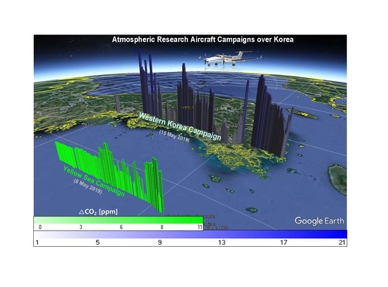
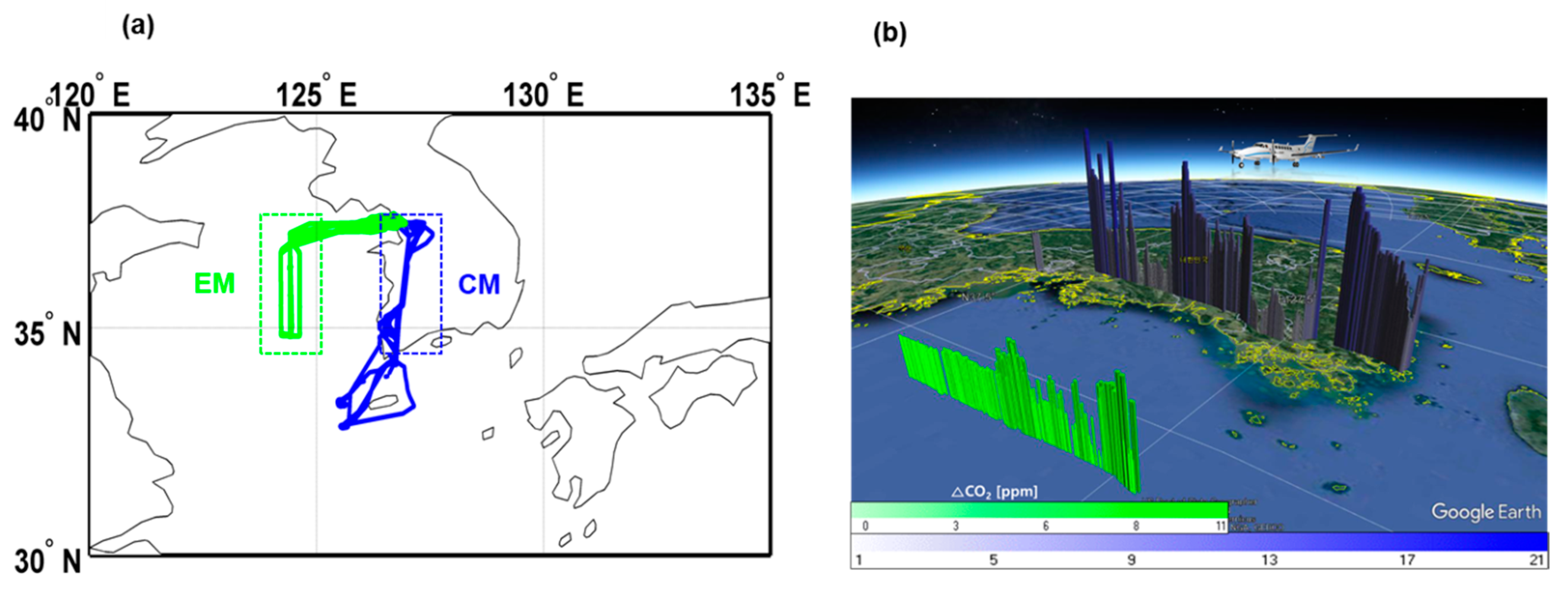
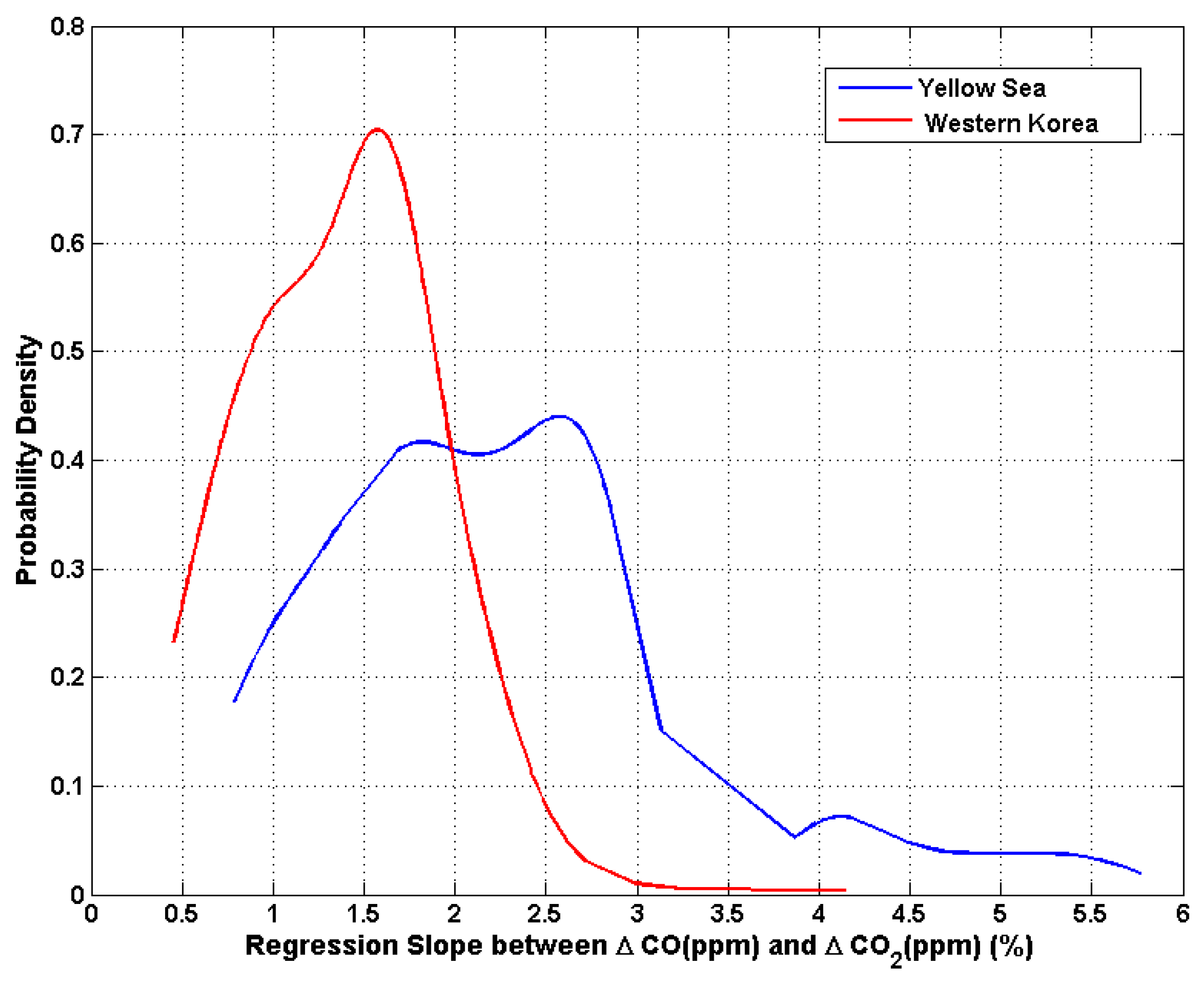
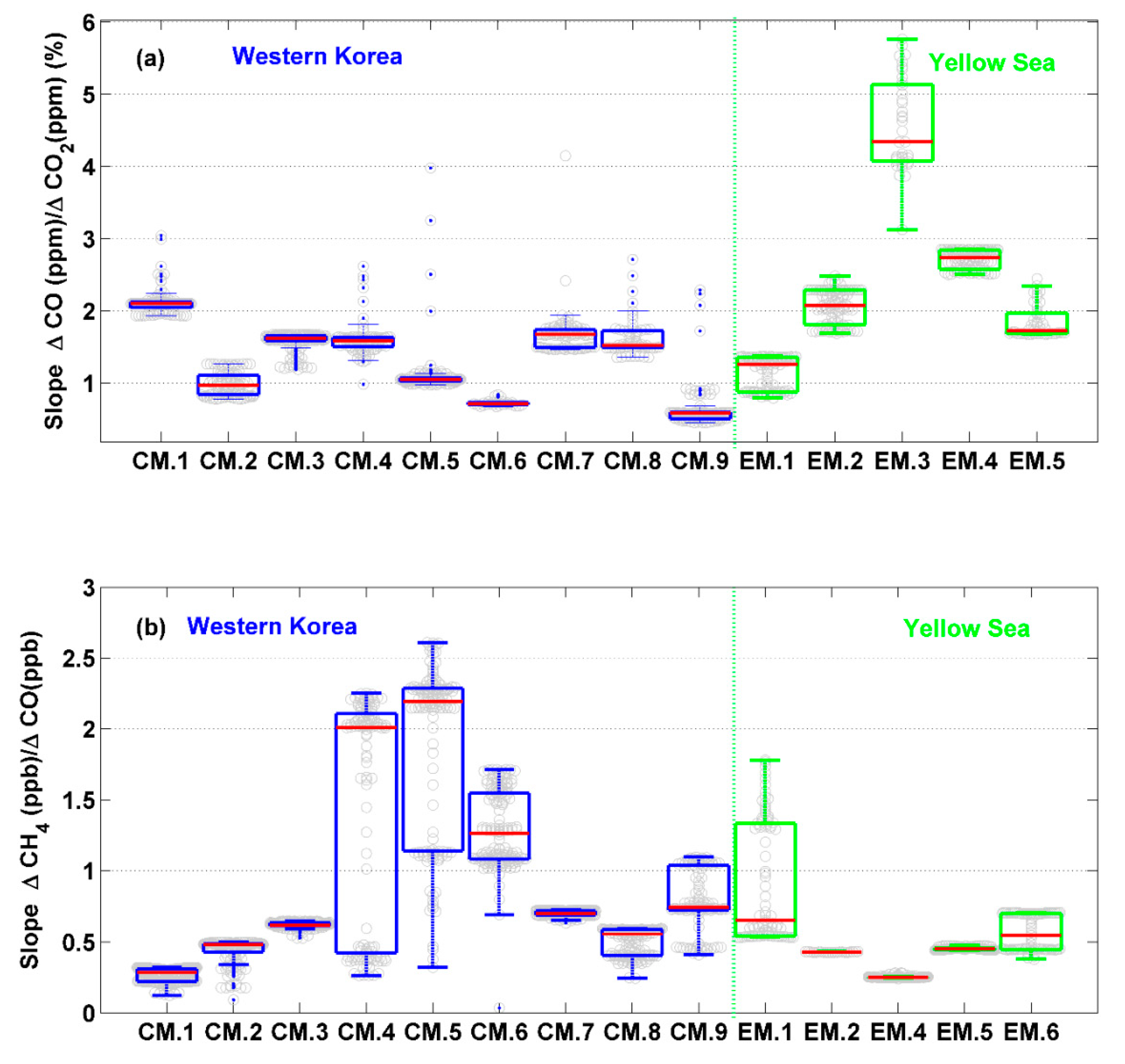
  • Characterizing air masses with the short-term (1-min) regression slope between ∆CO and ∆CO2 observed during the 14 flights campaign conducted in 2019 that covered Western Korea and Yellow Sea.
  • Characterizing the spatial and temporal variations of CO2 and CH4 across Western Korea where large clusters of CO2 and CH4 emission sources, such as industry, residual, and biogenic sources (such as agriculture, livestock, landfill, and so on), with the short-term (1-min) regression slope between ∆CH4 and ∆CO.
This study will improve understandings of the characteristics of CO2 and CH4 emission hotspots across Western Korea and build more confidence for inferring accurate and precise surface carbon fluxes over the region.

2. Materials and Methods
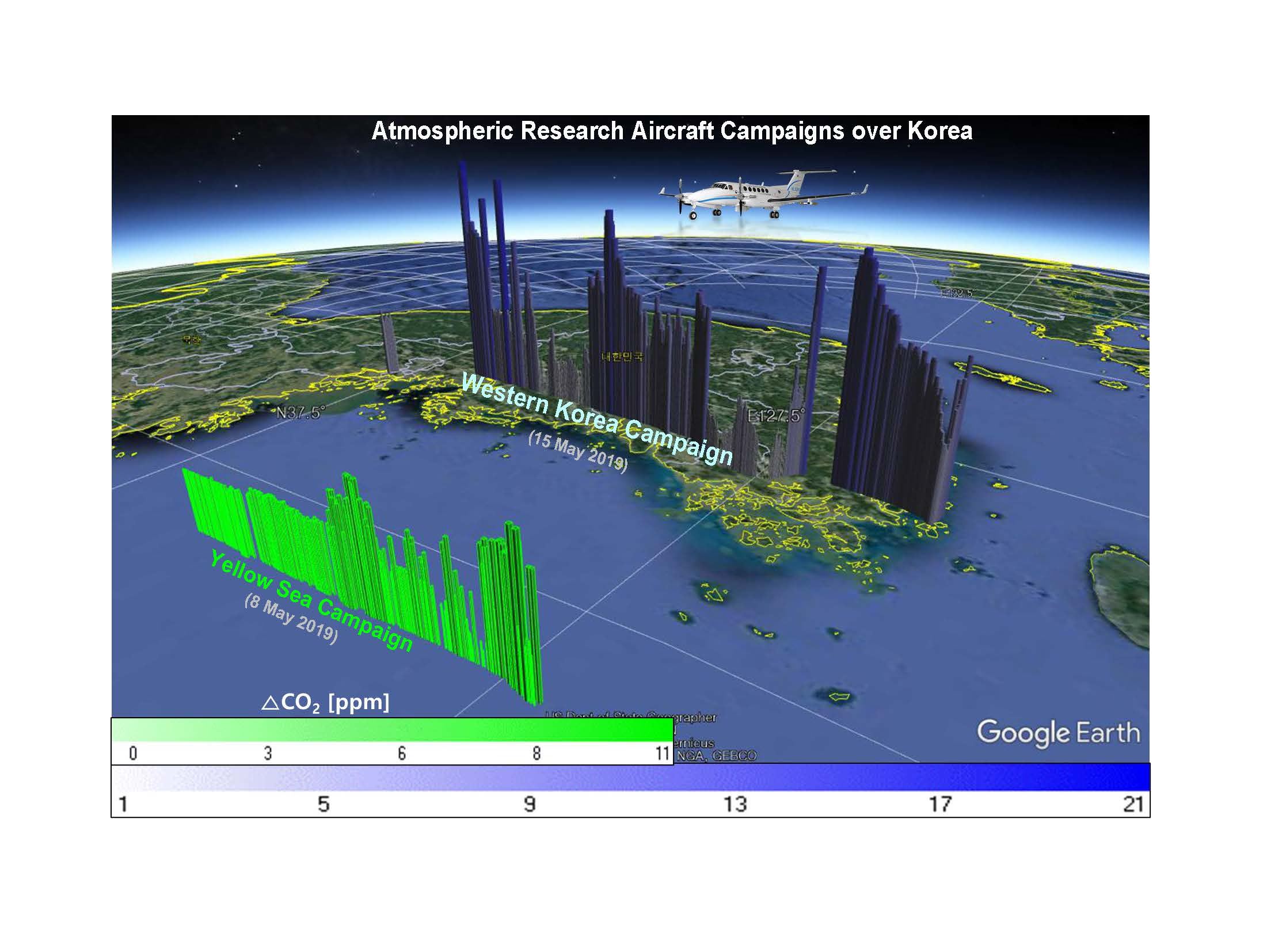
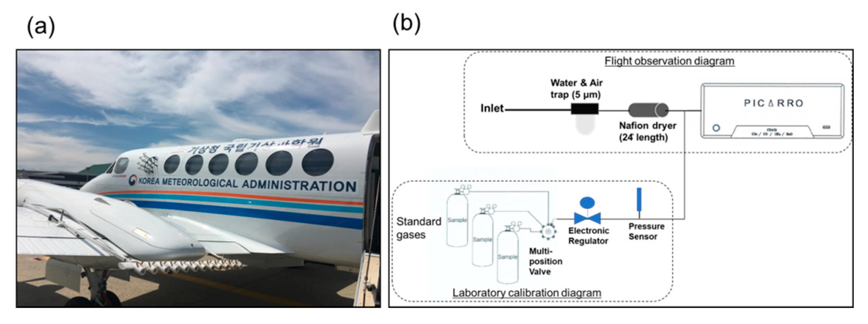
2.1. Aircraft

We used a KMA research aircraft based on the Beechcraft (Wichita, AR, USA) King Air 350 (Figure 1a) modified by Weather Modification Incorporated (Fargo, ND, USA). It has a ceiling of 9.6 km, speed range of 70–120 m/s, with a maximum flight time of 5.5 hours with the maximum payload. There are five seats: two for pilots, one for a scientist to manage the science missions, and two for the instrument operators. There are 24 instrumentations and one air inlet installed in the aircraft as shown in Table S1 of the supplementary materials (the payload of the King Air 350). The aircraft carries a Global Positioning System (GPS) that provides altitude and position information. Additionally, the Aircraft Integrated Meteorological Measuring System-20 was used to obtain basic meteorological data such as wind speed, wind direction, barometric pressure, vertical velocity, and so on.
The aircraft is equipped with a M300 data acquisition system (M300) to acquire and record measurement data. The M300 system enables real-time monitoring of the instruments operations and data acquisition. Data recorded by the individual instruments were finally combined into a single “merged sea file” with a time resolution of 1 s, which is available for each flight in addition to the instrument-specific data files. The single “merged sea file” can be converted into ASCII-format files to store the measurement data from individual instruments into separate files using Airborne Data Processing and Analysis, an open-source software package developed by the North Dakota University [18].

2.2. Aircraft Analyzer Setup and Calibration

The measurements employed a commercial analyzer developed by Picarro Inc. (CRDS, model G2401-m, Santa Clara, CA, USA) which simultaneously measures CO2, CH4, CO, and water vapor with high precision using a laser beam entering an optical cavity cell with highly reflective mirrors (optical path length of 15–20 km). CRDS measures the time constant of the decay (ring-down) of the light intensity as it is absorbed by the target gas in the optical cell after the laser is turned off. The instrument uses a high-precision wavelength monitor along with controlled pressure and temperature within the measurement cell to achieve high precision trace gas measurements. Compared to non-dispersive infrared (NDIR) instruments, CRDS is more stable and drift-free over short- and long-time scales.
The inlets delivering external air into the instrumentation are mounted through an aluminum plate on the first window of the fuselage of the aircraft; one for the CRDS analyzer, and others are for O3, SO2, NOx, and NOy analyzers (Figure 1a). A vacuum pump downstream of the CRDS analyzer pulls external air through the inlet and the analyzer. Upstream of the CRDS we installed a water/dust filter trap (5 μm) for removing water droplets and dust, and a three-way valve for pre-deployment calibrations (Figure 1b). The Nafion membrane dryer was installed upstream of the CRDS to remove water vapor included in the air sample (the detailed design of the Nafion dryer is described in Section 2.3).
The Picarro CRDS-G2401m was optimized to aircraft measurements and can accept inlet air close to or below the ambient pressure. Since pressure significantly exceeding one atmosphere causes instability in the pressure of the analyzer cavity cell, we constructed a pressure control system for standard reference tank calibrations. A rack-mounted auto-pressure controller (APC) contains a sample-selection rotary valve, a pressure sensor, and an electronic pressure regulator to maintain stable injection pressure with resolution of 0.1 bar to CRDS instrument, as shown in Figure 1b. Instruments were calibrated with APC by the following steps: first, the output pressure was roughly adjusted with a regulator installed in standard sample cylinders; second, each standard air sample was injected through the rotary valve automatically in 40 min based on the RS-232 communication method; third, the pressure was set in the electric panel of the pressure regulator approximately 0.5–0.7 bar above ambient pressure and the electronic pressure regulator automatically adjusted the pressure until the pressure was equivalent to that detected from the pressure sensor installed upstream of the CRDS. Then, the electronic pressure regulator could deliver pressure-controlled standard gases from the tank, and, thus, that could protect the sample cell from accidental excess pressures and ensure that the cavity did not have sensitivity from the injection pressure.
Three calibration tanks are connected via 1/8” OD stainless steel tubing to other ports on the rotary valve. The Picarro CRDS was calibrated more regularly and frequently (two-month intervals) in our laboratory, with a series of three World Meteorological Organization (WMO) scale standard sample tanks for CO2 (374.06, 419.45, and 467.78 ppm) and CH4 (1756.7, 1901.4, and 2325.8 ppb), two for CO (311.1 and 89.7 ppb) from NOAA/ESRL, with full coverage of the observed range of ambient air. Since the CO levels are low in the troposphere (i.e., ~50 ppb), zero gas has been included to adapt to the three points’ linear calibrations. Flight measurements for all three species are initially corrected using this linear calibration. The drift in the analyzer between laboratory calibrations in November and December 2018 were 0.03 ppm for CO2 and 0.9 ppb for CH4, which are nearly negligible levels of drift compared to inter-laboratory compatibility goals of WMO/GWA for CO2 (0.1 ppm for the northern hemisphere) and CH4 (2 ppb for the northern hemisphere). We conducted more frequent (two-month interval) NOAA/ESRL standard sample gas calibrations in the laboratory with a precise pressure controller of the APC calibration systems, as described above. Instrument precision was calculated from the average 1-σ standard deviation during approximately 30 min of the standard sampling and was 0.03 ppm for CO2, 0.1 ppb for CH4, and 2.2 ppb for CO.

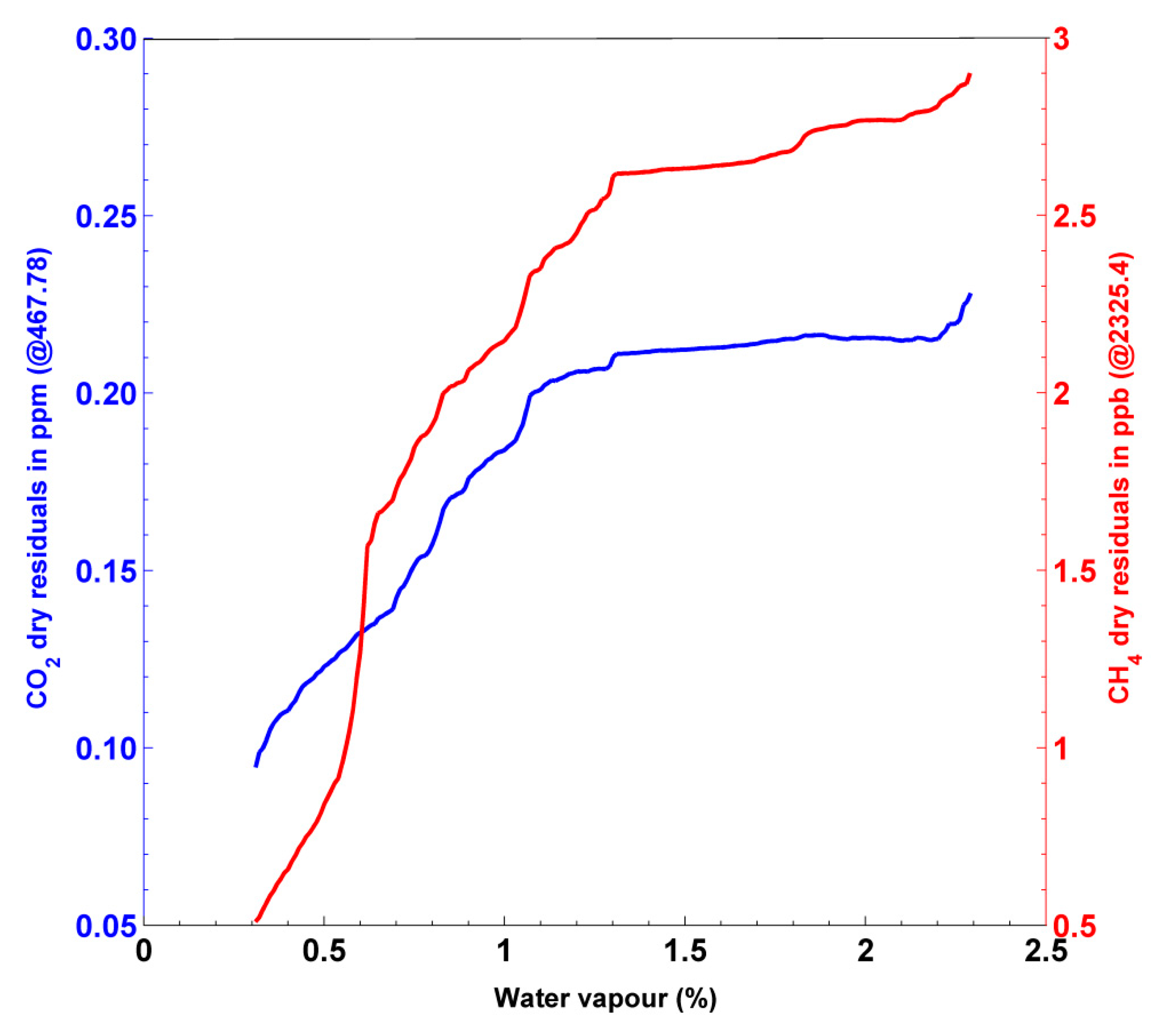
2.3. H2O Correction Error Analysis

The mixing ratio of CO2 and CH4, measured in terms of the wet-air mixing ratio, are significantly affected by the variations of water vapor due to the dilution effect. To avoid the dilution effect, CO2 and CH4 mixing ratios are reported as dry mole fractions using the correction parameter provided by the manufacturer. In our aircraft campaigns, the dry air mole fractions of CO2, CH4, and CO were calculated using the manufacturer-supplied correction factor. Thus, laboratory tests were performed to assess the water vapor correction error for the manufacturer-supplied correction factors by adding water vapor to dry standard sample gases from tanks at a mole fractions of 467 ppm for CO2 and 2325.4 ppb for CH4. The method described by Karion et al. [19] used a standard sample gas flowing through chamber (28.5 × 8 × 6.5; the size was designed to be able to mount on aircraft, detailed in Figure S1a of the supplementary materials) mounted with a Nafion membrane tube and a small humidifier of distilled water. Then, the water vapor is delivered to the gas stream which results in a smother water vapor transition across a range of approximately 0.3–2.3% (Figure 2).
The residuals between the NOAA standard gas mole fraction and those that responded to CRDS as changing water vapor concentrations are depicted in Figure 2. Residuals increased sharply at water vapor concentrations < 1%, then more gradually for water vapor concentrations > 1%. Additionally, the CO2 and CH4 changed by more than 0.2 ppm and 2 ppb (compatibility goals of WMO/GWA), respectively, for H2O values over 1%. As shown in Figure S2 of the supplementary materials, the H2O concentrations could be controlled below approximately 1% using the Nafion membrane dryer from October 2019 (no dryer was used before October 2019), however, the highest H2O concentrations in the summer (June through August) are as large as 2% without using the dryer. This indicates that the dry-mole fraction measurements after the installation of the Nafion filter are well within the GAW compatibility limits of water vapor concentration below 1% required for using the manufacturer-supplied correction factors, similarly to Rella et al. [20]. In our aircraft system, a simple purge gas-free Nafion membrane dryer was installed upstream of the CRDS to remove water vapor contained in air samples since 1 October 2019. By filling the chamber with silica gel to obtain dry conditions, as in Figure S1b of the supplementary materials, the water vapor contained in external air streams is removed via transition through the Nafion membrane. The silica gel was regularly replaced as its color changed.
Overall, we report uncertainties in the water vapor correction from the manufacturer-supplied correction factors of 0.28 ppm for CO2 and 2.7 ppb for CH4 for the period from June to August, and of 0.17 ppm for CO2 and 1.9 ppb for CH4 during other periods in this study. The uncertainty for CO was insensitive to water vapor within the water vapor range of 0.3–2.3% with 1-σ standard deviation of approximately 3 ppb.

2.4. Total Uncertainty Analysis

The total measurement uncertainty in this study was calculated by the combination of the CRDS instrumentation precision, water vapor correction errors, and the errors in the cavity pressure sensitivity. We performed pressure sensitivity experiments in the laboratory to simulate flight conditions over the pressure range of 320–1000 hPa and calculated the average 1-σ standard deviation during three hours of NOAA standard gas sampling (Figure S3 of the supplementary materials). We obtained 0.03 ppm for CO2, 0.5 ppb for CH4, and 3.0 ppb for CO. Overall, the uncertainties in the CRDS instrument were 0.17 ppm (0.28 ppm in summer), 1.9 ppb (2.7 ppb in summer), and 4.2 ppb for CO2, CH4, and CO, respectively, for 2019 by propagating all uncertainty terms (Table 1). Larger uncertainties are primarily attributed to the water vapor corrections in the summer season, making the Nafion dryer necessary. The NOAA standard-gases expanded uncertainties induced by the regulator and/or during the preparation of the secondary standard samples from the primary standards should be considered. This study accounted for both the aircraft instrumentation uncertainties and the expanded uncertainties of the standard gases (Table 1).
Time errors should also be corrected for each flight campaign. Cross-correction analyses were performed on pairs of observations from a single flight in order to assess the time-lag corrections for CRDS instruments because of the response time of CRDS in the M300 merging process. We found that the GPS time corresponds to the UTC time well and vary by no more than 1–2 s in each flight campaign. In addition, there are instrument delays in response to the residence time in the tube and water trap, which is on the order of magnitude of a few seconds. With the declared pumping rate of 350 cc/min and the cavity, tube, and water trap volume of 11.8 cc, there is approximately 2 s residence time. With a cruising speed of 70–90 m/s, this translates into spatial scales of approximately 140–180 m, which should be adjusted through manipulations of the flying regime. Finally, all of the CO2 and CH4 data analyzed in this study were adjusted by approximately 4 s for time-lag corrections introduced in the M300 merging process and the volume of the cavity, tube, and trap.

2.5. Scientific Aim and Flight Design

We designed two aircraft missions to collect major GHGs (CO2, CH4, and H2O) and an indirect GHG (CO): first, climate change monitoring (CM) missions that research aircraft was flown from the aircraft’s home base at Gimpo airport near the Seoul megacity to conduct a low-altitude (about 1 km above mean sea level (amsl), mostly within the boundary layer) survey on a south-north path between about 34°N and 37°N over the Western Korean land region, which included metropolitan, urban, and rural regions (Figure 3). A total of nine one-day flights were carried out in 2019 (Table 2). The primary scientific goal of this mission was to investigate the distribution of CO2 and CH4 within the boundary layer over Korea for all seasons. The high-resolution data can provide information on various sources and sinks of particulates and trace gases in the region and can be utilized in inversion simulations coupled with an atmospheric transport model to quantify the GHG budgets in Korea.
Second, an environmental monitoring (hereafter EM) mission was flown out of the aircraft’s home base at Gimpo airport to conduct a low-altitude (~600 m amsl, mostly within the boundary layer) survey over the Yellow Sea to monitor the westerly trans-boundary pollutants transports (Figure 3). The primary scientific goal of this mission was to understand long-distance transports of atmospheric pollutions from China into Korea across the Yellow Sea. This study analyzed the measurements during the period from April to May 2019 from the EM mission.
Typical campaigns started from noon and continued for approximately four hours, the periods when the boundary layer heights are at their maximum. Table 2 provides a summary of flight information including the dates, duration of flights, the maximum and minimum temperature measured in the aircraft, and the CO2 and CH4 for all flights. In this study, we analyzed the aircraft-measured atmospheric CO2, CH4, and CO over Korea in 2019 for both missions. Typical EM and CM missions are usually conducted over different routes and periods, however, all measurements are expected to be combined for interpretations. We also conducted a special campaign that combines the CM and EM mission route when super Asian dust or fine dust events are forecasted to occur over the Yellow Sea and Korea.
Separately, the atmospheric vertical profiles are measured for altitude range between 0.6 km and 9.0 km over the AMY station (36.53°N, 126.32°E), a GAW regional background station [14], coincided with overpasses of the Greenhouse Gases Observing Satellite (GOSAT). Li et al. [16] found that the CO2 observed in the free troposphere, 1.5–8 km above the mean sea level, in 2018 are smaller than the AMY GAW surface station data in spring but agree closely in summer; however, the CO2 are consistent with the aircraft measurements over the Western Pacific conducted by the Japan Meteorological Agency. They also found that the free-tropospheric CH4 was smaller than those from the surface AMY station. Li et al. [16] also analyzed the long-range CH4 transport mechanism in the free troposphere. The additional studies are currently in progress using the aircraft AMY spiral mission data: a validation of satellite retrieval and a comparison to the background level observed from the AMY GAW station. This will be discussed in future studies.

2.6. Short-Term Regression Slope Calculation Method

The CO2, CH4, and CO have background seasonal gradients, reflecting their sources, OH concentration, and vegetation fluctuation. To remove the influence of these background gradients, the CO2 and CH4 at low altitude (~1 km amsl) deducted their mole fractions measured in free troposphere (2–8 km) [16,21], which were defined as “background”. The measurements with this background removed (denoted by ∆) are greatly affected by source and sink strength surrounding the aircraft route.
The regression slope between ∆CO and ∆CO2 has been used extensively to characterize regional source signatures, as the majority of atmospheric CO comes from incomplete combustion of carbon-containing fuel [22]. Thus, high-efficiency combustion converts fuel carbon almost entirely into CO2, producing low regression slopes, and vice versa. Generally, Korea has stricter vehicle emissions standards than China [23]; however, combustion efficiency has been increasing in China with improved emissions control technology and government pollution control actions [24,25]. Thus, we compared the regression slope between ∆CO and ∆CO2 observed in different flight routes (CM and EM campaigns) to determine if the emission sources are located in China or Korea. Recently, short-term continuous slopes (1-min slope based on one second data) between high-resolution CO2 and CO aircraft measurements provided regional fingerprints for assessing emissions and mixing behaviors [26]. The regression slopes between ∆CH4 and ∆CO are also investigated, and it may be attributable mainly to seasonality in this region.
Short-term (1-min) regression slopes between ∆CO and ∆CO2, ∆CH4 and ∆CO were calculated using the Williamson-York linear least-squares fitting methods [27,28], which considers measurement uncertainties as shown in Table 2. With a cruising speed of 70–90 m/s in the CM and EM campaign, 1-min aircraft data translates into spatial resolutions of approximately 4–5 km. The slopes were calculated with a 1-min window based on one second data, filtered by the correlation coefficient (cut-off range of p < 0.01, R2 > 0.4). For details refer to Halliday et al. [26]. The cut-off value of R2 was determined as the calculated uncertainties, as summarized in Table 3. We considered uncertainties with a R2 above the cut-off values (R2 > 0.4) to be sufficiently small, therefore, the slope with R2 values above this cut-off value were considered to be effectively correlated and, therefore, are included in the analysis.

3. Results and Discussion

3.1. Regional Source Characteristics Using Regression Slope between Short-Term (1-min) ∆CO and ∆CO2 Data

3.1.1. Yellow Sea Receptor Analysis

Figure 4 shows the distribution of regression slope in percentages (above the R2 cut-off values) between ∆CO (ppm) and ∆CO2 (ppm) calculated for all flights in the CM and EM campaign. A majority of slope values occur between 0.5% and 2.5% and 1.6% and 5.5% for CM and EM flights, respectively. Over 66% of the slope in CM are between 1% and 2%, with only 11% of the slope exceeding 2%. In contrast to CM, over half of the slope in EM are above 2% with 11% exceeding 4%. Overall, the slope in EM are approximately 2–3 times larger than those in CM, indicating that observations observed in EM are associated with more inefficient combustion sources than in the CM campaign.
Figure 5 summarizes the dynamic ranges of the regression slope in Figure 4 according to the flight time and missions. It is noted that all of the regression slopes between ∆CO and ∆CO2 below 1.5% occurred on 16 April, and all of the RS between 3% and 6% occurred on 8 May in the EM campaign (Figure 5). A majority of the slopes fall between 2% and 3% for other flights while the regression slopes with R2 exceeding the cut-off value (<0.4) were not observed on 3 May. We investigated the air mass origins using the six-day backward trajectories calculated with the NOAA HYbrid Sing-Particle Lagrangian Integrated Trajectory (HYSPLIT) model for the EM flights to categorize the slope with emission influenced region (Figure 6a–f). The HYSPLIT model developed by NOAA/ERSL is widely used to generate backward trajectories of the origin of air masses and establish source-receptor relationships for the given initial locations. The model using the Lagrangian framework compute the time integrated advection of each particle can be viewed as a simple trajectory which requires the three-dimensional velocity field from the Global Data Assimilation (GDAS) dataset obtained from the National Centers for Environmental Prediction (NCEP) by the Air Resources Laboratory, detailed in [29].
The six-day back-trajectories mainly passed through the Korean peninsula on 16 April, the day in which the smallest regression slopes (<2%) in EM are found, whereas back-trajectories on other EM days go through Eastern China. It clearly shows that trajectories stagnated for ~3 days over a large area in Eastern China including Jiangsu, Shandong, and Hebei provinces within the boundary layer before arriving at the sampling sites on 8 May (Figure 6d), indicating the influence of inefficient combustion sources in Eastern China. The higher mixing ratios of CO in the sampling regions appear to indicate the influence of the industrial sector in Hebei and Shandong regions because the emission inventory for the Chinese industrial sectors have expected ratios of 3–4% [26]. The regression slopes observed on 8 May are also close to those observed in Beijing (~4%) and Nanjing areas in China [30,31], indicating that the large regression slope can be greatly attributed to inefficient combustion sources in those area. This is also consistent with the regression slope between ∆CO and ∆CO2 calculated with satellite measurements; the value is much lower for the Seoul region than over the metropolitan areas in China and Japan [32].
The regression slopes in the cases affected by more efficient combustion compared to the 8 May case were sampled on the EM missions on 19 April and 21–22 May ranges from 1.8 to 2.9% (Figure 5). In these cases, air masses from Eastern China and Northern China rapidly moved through the sampling locations over the Yellow Sea (Figure 6c,d). These values are close to the annual average regression slope during 2017–2018 observed in Shanghai (1.8–2.1%), representing combustion sources such as vehicle exhaust and gas-fired power plants [25]. In summary, moderate westerly flows from East-central China, including Shandong and/or Hebei province, most likely contributed to a higher regression slope between ∆CO and ∆CO2 (>3%) from industrial sectors. This result was similar to the finding by Lee et al. [33] that showed the air pollution from East-central China usually contributes towards high levels of air pollution concentrations in Korea. We investigated the regression slopes between ∆CO and ∆CO2 originating in Korea and China to find that combustion sources in Korea are generally more efficient than those in China. More detailed analyses of the characteristics of combustion sources in various regions and emission sources are a subject of future research.

3.1.2. Western Korea Receptor Analysis

In contrast to the Yellow Sea EM campaign, the Western Korea CM campaign was designed for sampling of domestic pollution so as to identify the main monthly GHGs hotspots over the Western Korea. We investigated the regression slope calculated for each CM flight (Figure 4) to determine if the observations are associated with emissions in Korea by comparing the regression slope against that associated with a typical Chinese emission source in the EM campaign. The regression slope between ∆CO and ∆CO2 mostly represented the aircraft data sampled at an altitude of approximately 1 km amsl along Western Korea, however, on some occasions the aircraft flew above 1 km amsl due to air traffic control. Overall, most of the flights are below or near the boundary layer except the flights in southern regions in June, and, therefore, could represent background samples in the low free troposphere (details shown in Figure S4, regression slopes between ∆CO and ∆CO2 for each CM flight missions, the ECMWF-ERA5 derived and observed in the boundary layer).
Most of the regression slopes between ∆CO and ∆CO2 in the CM mission are less than 2%, representing efficient combustion sources, whereas it was distributed between 1.9–3.1% in January which represent inefficiency combustion emission when a stronger northwesterly wind speed ranged between 6–12 m/s than that in other season while wind ranged below 6 m/s (Figure 7). This suggests that exhaust from inefficient combustion emissions were transported from China in January with strong winds. Most of the regression slope values below 1% were observed in August and December, and regression slopes for other months ranged between 1% and 2% ∆CO/∆CO2. As shown by the regression slope distributions observed during EM missions, the long-transported CO and CO2 from China shows inefficient combustion sources with regression slope above 2% and from Korea shows efficient combustion sources with regression slope below 1.5%. Thus, CM campaign measurements appeared to be mostly connected to Korean domestic emission sources with wind speeds below approximately 6 m/s (Figure 7). This is also consistent with results from KORUS-AQ campaign that showed that 80% of the regression slope between ∆CO and ∆CO2 observed in Seoul fell between 0% and 2% and Chinese emission sources have a regression slope range of 2–4% [26]. Noticeably, outlier slopes above the 95th percentile were frequently observed during CM scientific flights, and higher regression slopes (>2%) were observed near 36–37°N latitude of Korea (e.g., Seoul, Gyeongi-do, etc.; refer to Figure S4 of the supplementary materials). It is interesting that higher regression slopes between ∆CO and ∆CO2 were observed within the boundary layer in January, July, and November and through the lower free troposphere occurring in October and December (Figure S4). This indicates that Northern Korea (Seoul, Gyeonggi-do) was more frequently affected by inefficient combustion sources than Southern Korea not only under the boundary layer but also through the lower free troposphere.

3.2. Spatio-Temporal CO2 and CH4 Variations over Western Korea

The horizontal distributions of atmospheric CO2 and CH4 for 2019 over Western Korea within the latitude range of 34–37°N for 2019 are shown in Figure 8. To present the spatiotemporal distributions of CO2 and CH4 more clearly, their mole fractions were measured within the boundary layer are averaged at latitude bins of 0.075° and temporally interpolated with aircraft sampled time.
The CO2 shows clearly the zonal and seasonal distribution characteristics, with high CO2 levels in Northern Korea which includes densely populated urban and industrial regions, such as Seoul, Gyeonggi-do, and Chungcheong-do, and low levels in the southern part near Jeolla-do which includes large agricultural lands and forests (Figure 8a). This also indicates that the flight mission successfully captured the variations in the concentration level according to regional emissions sources.
Table 4 summarizes the observed mean level of CO2 and CH4 below 1 km amsl, for the entire CM campaign. The maximum and minimum CO2 are found in April (420.6 ± 3.4 ppm) and August (399.5 ± 4.7 ppm), respectively. Although the CM mission was unable to cover the whole day of each month, that the observed values compare well with the observations at AMY and Gosan (33.30°N, 126.16°E) GAW background stations in Korea, which show a minimum in August and a maximum in April [14]. As per a previous study, the CO2 observed in the vicinity of megacity regions (Nanjing, Beijing, Shanghai, and Lin’an) showed high levels in winter, but in spring in remote stations (AMY, Gosan, Waliguan, and Shangdianzi) in Northeast Asia [14,34]. This is likely due to stronger biogenic emissions in spring with rising air temperature in rural and remote sites compared to densely-populated urban sites with higher fossil fuel emissions in winter. Our CM campaigns covered all rural, urban, and suburban regions, and, therefore, present the average atmospheric CO2 level in Korea which mixed with different emission sources and sinks.
Conversely, CH4 showed high levels in the southern region in the vicinity of Jeollanam-do (35.0~34.0°N) for the period of July through August, followed by Gyeonggi-do (36.1~36.9°N) and Chungcheong-do (36.9~37.5°N) in May and August (Figure 8b). The average of CH4 was the highest in August 2019 (2071.4 ± 63.1 ppb), followed by July (2019.4 ± 79.7 ppb) and May (2006.3 ± 47.3 ppb), and was the lowest in January (1942.5 ± 27.4 ppb), followed by October (1949.7 ± 37.5 ppb). Assuming that observations in January represented the long-transported sources from China, as shown in the regression slope between ∆CO and ∆CO2, the average patterns are similar to those of other nearby urban (e.g., Shanghai megacity in China) and remote stations (AMY in Korea), with a peak in August and a trough in October. As Shim et al. [35] report, CH4 flux measured using the open/close chamber method peaked in June–July during the rice paddy tillering stage, followed by the elongation stage from July to August in the southern part of Korea. This is consistent with the CM aircraft measurement which showed higher levels around Jeolla-do during the July period. According to national bottom-up inventory reports, >40% of Korean CH4 emissions were emitted from agriculture, followed by landfill (31%) and energy consumption (22.9%) [36]. Rice paddies are the largest CH4 source in the agriculture sector, and 54% of total agriculture land is used for rice paddies in Korea [37]. As for the previous results, the western region of South Korea showed a trend toward higher CH4 emissions than the eastern region because the top 15 administrative cities with high CH4 emissions emitted from rice paddies are all located in Western Korea (for further detail, see Choi et al. [38]). Thus, CM missions clearly captured the seasonal and spatial gradients using the first in situ aircraft measurements.
The aircraft measurements operated at an altitude of approximately 1 km amsl before arriving at Jeolla-do (35.5–34.0°N) in June. Thus, it is not possible to present the zonal gradient in the boundary layer in June, especially in the northern part of Korea. However, measurements in other periods thoroughly covered the boundary layer and the average wind speeds during this period were less than 6 m/s (Figure 7). Thus, CO2 and CH4 emitted from local sources accumulated under stable weather conditions and minimized the effect of atmospheric long-transport by wind for this period. To characterize the CH4 emissions sources, the regression slope between ∆CH4 and ∆CO were also calculated with the Williamson–York linear least-squares fitting method, and were filtered by the coefficient (cut-off values of p < 0.01, R2 > 0.4). Given that air masses affected by EA fossil fuel, regression slope showed approximately 0.2–0.4 in winter observed at the Hateruma Island remote site in Japan [39], the slopes observed in January and May clearly exhibit fossil fuel source emission patterns. Given that the regression slope between ∆CH4 and ∆CO observed in the urban region were in the range of 0.55–0.76 [40,41,42,43] in which the typical urban sources such as landfill, oil and gas extraction emissions were mixed, the regression slope between ∆CH4 and ∆CO slopes observed on April, May, and October–December are mainly attributed to urban emissions sources from Korea along with the west regions.
Obviously, the regression slope between ∆CH4 and ∆CO was broadly distributed between 0.5 and 2.3 in June–August in the summer season during CM missions, which is a similar pattern to the slope of 0.5–2.0 in summer at Hateruma station. The higher slope in summer, i.e., nearly reaching a 2.3 slope, was mainly attributed to the maximum CH4 emissions from rice paddies not arising from fossil fuels, biofuels, or biomass burning [44]. The regression slope distributions observed in August were less broad than those from June to July and a high level were evenly distributed from northern to southern parts of Korea (Figure 8), which indicates that influences from other biogenic sources (landfill and livestock) become stronger as the temperature increases in August than those observed in June–July. It is also noteworthy that CO distributions and hotspots observed during the entire CM campaign were consistent with the CH4 horizontal distributions (Figure S5 of the supplementary materials). Given that CH4 oxidation contributes to 28% of the tropospheric CO burden [45], it cannot be ruled out that the CO source is oxidation of CH4 in the summer in Korea, a trajectory in which the correlation between CO and CH4 is significantly stronger in summer (R2 > 0.7) that is also plausible. However, more detailed studies need to be continued to identify CO emissions sources in Korea, especially in summer, using chemical model simulations. This was beyond the scope of this study and will be discussed in future studies.

3.3. Comparison with Backgrounds

Next, we investigated the difference between CO2 and CH4 observed throughout the entire CM campaign, and background, which were calculated with observations in the free-roposphere (detailed in Section 2.6). GHGs obtained in the CM mission represent the atmospheric CO2 and CH4 levels that are affected by local emission sources. The differences between CO2 and CH4 can provide the strengths of potential carbon sources and sinks against the global marine surface background level.
The distributions of differences between 1-min average CO2 and CH4 according to latitudes obtained during the nine campaigns over Western Korea, as well as the mean background level, are plotted in Figure 9. The difference, ∆CO2, between the average CO2 obtained during the nine campaigns over Korea and the mean background CO2 levels is high in spring (>5 ppm, 1.2% higher than the background level) and low in August, indicating that strong sources and sinks existed in this period over Western Korea. The highest values appeared in the northern region throughout the whole campaign, whereas strong CO2 absorption with a difference range between 0 and −10 ppm was concentrated in Southern Korea for the period July through August. This can be attributed to strong sinks of cropland, the third largest carbon sink in Asia [46,47]. The higher ∆CO2 in the northern parts compared to the southern parts were associated with the presence of large emission sources related to combustion in the northern part.
For CH4, the largest differences of nearly 250 ppb occurred for the period of July through August. Extreme high CH4 observed in this period were approximately 6% higher than the background level, suggesting significant CH4 sources in Southern Korea from biogenic sources. Characterizing the temporal variations of the main CH4 emissions sources such as crop growing, landfill, and fossil fuels using a combination of aircraft measurements, model simulations, and isotope measurements will be useful for reducing atmospheric CO2 as well as CH4, the second most important anthropogenic greenhouse gas.

4. Conclusions

This study firstly describes an in-depth investigation of CO2, CH4, and CO data over Korea measured using a new research aircraft, a Beechcraft King Air 350, under the KMA-Atmospheric Research Aircraft Program for 2019. We constructed a simple CRDS onboard system and the estimated uncertainties in the CRDS instrument were 0.17 ppm (0.28 ppm in summer), 1.9 ppb (2.7 ppb in summer), and 4.2 ppb for CO2, CH4, and CO, respectively, for 2019 by propagating all uncertainty terms, such as instrument precision, uncertainties in cavity pressure sensitivity, and water vapor correction error. Larger uncertainties are primarily attributed to the water vapor corrections by manufacture provided water vapor correction factors in the summer season, making the Nafion dryer necessary.
We analyzed the aircraft-measured atmospheric CO2, CH4, and CO over Korea in 2019 with two different missions. The first mission was as follows: the research aircraft conduct a low-altitude (about 1 km amsl, mostly within the boundary layer) survey on a south-north path between about 34°N and 37°N over the Western Korean land region that include metropolitan, urban, and rural regions. The second mission are targeted to measure atmospheric pollution over the Yellow Sea to monitor the westerly trans-boundary pollutants transport.
To characterize the regional combustion sources signatures of CO2 and CH4, we calculated the short-term (1-min slope based on one second data) regression slope of CO to CO2 enhancements (∆CO, ∆CO2, and ∆CH4) with the Willam–York linear least square method, considering measurement uncertainties of CO and CO2; regression slopes were filtered with correlation coefficients (R2) (<0.4 were ignored). These short-term slope analyses seem to be sensitive to aircraft measurements in which the instrument sampled short-time varying mixtures of different air masses. The Yellow Sea missions, all of which were affected by pollutants emitted in China, show the regression slope between ∆CO and ∆CO2 with of 1.8–6%. In particular, the regression slope between ∆CO and ∆CO2 increased to >4% when air flows from East-central China such as Hebei, Shandong, and Jiangsu provinces, etc., sustained for 1–3 days, suggesting pollutants from these regions were most likely characterized by incomplete fossil fuel combustion from industry. Over 80% of the observations in Western Korea inland were attributed to Korean emission sources with a regression slope between ∆CO and ∆CO2 of 0.5–1.9%. Overall, the regression slope of the Yellow Sea are approximately 2–3 times larger than those in Western Korea, indicating that the samples from the Yellow Sea are associated with more inefficient combustion sources than in Western Korea. Additionally, we characterized the spatial and temporal distributions of CO2 and CH4 within a boundary layer across Korea, specifically, the western part. Extremely high CH4 observed in Korea during the summer were approximately 6% higher than the background level, suggesting that significant CH4 sources occurred in Southern Korea from biogenic sources, such as agricultural activity (especially rice paddies), landfill, livestock, and so on. Characterizing the temporal variations of the main CH4 emission sources, such as crop growing, landfill, and fossil fuels, using a combination of aircraft measurements, model simulations, and isotope measurements, will be useful for reducing atmospheric CH4, the second most important anthropogenic greenhouse gas.
Using the research aircraft, we continue to conduct in situ CO2, CH4, and CO measurements under the long-term KMA-Atmospheric Research Aircraft Program with high-density and high-precision that cover inland Western Korean and the Yellow Sea. Thus, the aircraft observations can provide a useful high-density dataset to better understand the CO2 and CH4 emissions source characteristics in Korea and their trans-boundary transport mechanism across the Yellow Sea. Further, the in situ CO2 aircraft observation data will be used for improving carbon flux estimations across Western Korea by combination model simulation; this will give insight for decision-making regarding the reduction of anthropogenic emissions of greenhouse gases in EA, especially in Korea and China.

Supplementary Materials

The following are available online at https://www.mdpi.com/2072-4292/12/18/3093/s1, Figure S1: Photo of the Nafion membrane installed chamber (a) without and (b) with silica gel dryer; it was designed for the Korean Meteorological Administration (KMA) research aircraft King Air 350 cavity ring-down spectroscopy (CRDS) measurements; Figure S2: Cavity ring-down spectroscopy (CRDS) reported water vapor concentration ranges (%) for all climate change monitoring (CM) missions for 2019; Figure S3: The CO2 dry mole fractions corresponding to NOAA standard gas at concentration of 467.78 ppm for CO2 with gradually decreasing inlet pressure ranges of 280–1000 hPa; Figure S4: Regression slope between ∆CO and ∆CO2 along the flight route and flying altitude above mean sea level (amsl), the dotted line shows the ECMWF ERA5 derived from the boundary layer at longitude 126.5–127°E and UTC time (0300–0700). However, the boundary layer height on the CM.2 mission was calculated with the King Air aircraft observed potential temperature difference and relative humidity because the ECMWF derived from the boundary layer seems to be underestimated; Figure S5: Spatiotemporal distributions of CO for all climate change monitoring (CM) missions. This figure depicts the CO concentrations measured within the boundary layer are averaged at the latitude bins of 0.075° (approximately 5-km spatial resolutions) and temporally interpolated with the aircraft sampled time (all the aircraft sample times denoted by CM.1 through CM.9 are provided in Table 4); Table S1: The instrumentation installed on a Korean Meteorological Administration (KMA) research aircraft based on Beechcraft King Air 350.

Author Contributions

Conceptualization, S.L., Y.K., J.K., S.T.K., L.D.L., T.-Y.G. and Y.-H.B.; methodology, S.L. and T.-Y.G.; software, S.L. and Y.K.; validation and formal analysis, S.L., Y.K., J.K., S.T.K., L.D.L.; investigation, resources and data curation, S.L. Y.K. and T.-Y.G.; Writing—original draft preparation: S.L. and T.-Y.G.; writing—review and editing: Y.K., J.K., S.T.K., L.D.L. and Y.-H.B.; visualization, S.L. and Y.K.; supervision and project administration, S.L. T.-Y.G. and Y.-H.B.; funding acquisition, T.-Y.G. and Y.-H.B. All authors have read and agreed to the published version of the manuscript.

Funding

This research was funded by the Korea Meteorological Administration Research and development Program “Development of application technology on atmospheric research aircraft” under grant (KMA2018-00222).

Acknowledgments

The authors would like to thank the pilots, payload operation team, ground-based technicians, and KMA’s research aircraft management team for their great contribution for our KMA aircraft missions. We thank ECMWF ERA5 team for providing meteorological reanalysis data and NOAA Air Resources laboratory for the provision of the HYSPLIT transport and READY website (http://www.ready.noaa.gov).

Conflicts of Interest

The authors declare that they have no competing interests.

References

  1. Callendar, G.S. Variations of the amount of carbon dioxide in different air currents. Q. J. R. Meteorol. Soc. 1940, 66, 395–400. [Google Scholar] [CrossRef]
  2. Bishof, W. Variations in concentration of carbon dioxide in the free atmosphere. Tellus 1962, 14, 87–90. [Google Scholar]
  3. Keeling, C.D.; Harris, T.B.; Wilkins, E.M. Concentration of atmospheric carbon dioxide at 500 and 700 milibars. J. Geophys. Res. 1968, 73, 4511–4528. [Google Scholar] [CrossRef]
  4. Houweling, S.; Rockmann, T.; Aben, I.; Keppler, F.; Krol, M.; Meirink, J.F.; Dlugokencky, E.J.; Frankenberg, C. Atmospheric constraints on global emissions of methane from plants. Geophys. Res. Lett. 2006, 33, L15821. [Google Scholar] [CrossRef] [Green Version]
  5. Frankenberg, C.; Bergamaschi, P.; Butz, A.; Houweling, S.; Meirink, J.F.; Notholt, J.; Petersen, A.K.; Schrijver, H.; Warneke, T.; Aben, I. Tropical methane emissions: A revised view from SCIAMACHY onboard ENVISAT. Geophys. Res. Lett. 2008, 35, L15811. [Google Scholar] [CrossRef] [Green Version]
  6. Ganesan, A.L.; Schwietzke, S.; Poulter, B.; Arnold, T.; Lan, X.; Rigby, M.; Vogel, F.R.; van der Werf, G.R.; Janssens, G.-M.; Boesch, H.; et al. Advancing scientific understanding of the global methane budget in support of the Paris Agreement. Glob. Biogeochem. Cycles 2019, 33, 1475–1512. [Google Scholar] [CrossRef]
  7. Gregg, J.S.; Andres, R.J.; Marland, G. China: Emissions pattern of the world leader in CO2 emissions from fossil fuel consumption and cement production. Geophys. Res. Lett. 2008, 35, L08806. [Google Scholar] [CrossRef]
  8. Peters, G.P.; Marland, G.; Quere, C.L.; Boden, T.; Canadell, J.G.; Raupach, M.R. Rapid growth in CO2 emissions after the 2008–2009 global financial crises. Nat. Clim. Chang. 2012, 2, 2–4. [Google Scholar] [CrossRef]
  9. Labzovskii, L.D.; Mark, H.W.L.; Kenea, S.T.; Rhee, J.S.; Lashkari, A.; Li, S.; Goo, T.-Y.; Oh, Y.-S.; Byun, Y.-H. What can we learn about effectiveness of carbon reduction policies from interannual variability of fossil fuel CO2 emission in East Asia. Environ. Sci. Policy 2019, 96, 132–140. [Google Scholar] [CrossRef]
  10. Li, S.; Kim, J.; Park, S.; Kim, S.-K.; Park, M.-K.; Mühle, J.; Lee, G.; Lee, M.; Jo, C.O.; Kim, K.-R. Source identification and apportionment of halogenated compounds observed at a remote site in East Asia. Environ. Sci. Technol. 2014, 48, 491–498. [Google Scholar] [CrossRef]
  11. Lee, G.; Oh, H.-R.; Ho, C.H.; Kim, J.; Song, C.-K.; Chang, L.-S.; Lee, J.-B.; Lee, S. Airborne measurements of high pollutant concentration events in the free troposphere over the West Coast of South Korea between 1997 and 2011. Aerosol Air Qual. Res. 2016, 16, 1118–1130. [Google Scholar] [CrossRef] [Green Version]
  12. Lee, H.-J.; Jo, H.-Y.; Kim, S.-W.; Park, M.-S.; Kim, C.-H. Impacts of atmospheric vertical structures on transboundary aerosol transport from China to South Korea. Sci. Rep. 2019, 9, 13040. [Google Scholar] [CrossRef] [PubMed]
  13. Tang, W.; Emmons, L.K.; Arellano, A.F., Jr.; Gaubert, B.; Knote, C.; Tilmes, S.; Buchholz, R.R.; Pfister, G.G.; Diskin, G.S.; Blake, D.R.; et al. Source contributions to carbon monoxide concentrations during KORUS-AQ based on CAM-chem model applications. J. Geophys. Res. Atmos. 2019, 124, 2796–2822. [Google Scholar] [CrossRef]
  14. Lee, H.; Han, S.-O.; Ryoo, S.-B.; Lee, J.-S.; Lee, G.-W. The measurement of atmospheric CO2 at KMA GAW regional stations, its characteristics, and comparisons with other East Asian sites. Atmos. Chem. Phys. 2019, 19, 2149–2163. [Google Scholar] [CrossRef] [Green Version]
  15. Li, S.; Park, S.; Lee, J.-Y.; Ha, K.-J.; Park, M.-K.; Jo, C.J.; Oh, H.; Mühle, J.; Kim, K.-R.; Montzka, S.A.; et al. Chemical evidence of inter-hemispheric air mass intrusion into the Northern Hemisphere mid-latitudes. Sci. Rep. 2018, 8, 1–7. [Google Scholar] [CrossRef] [Green Version]
  16. Li, S.; Goo, T.-Y.; Moon, H.; Labzovskii, L.; Kenea, S.T.; Oh, Y.-S.; Lee, H.; Byun, Y.-H. Airborne in-situ measurement of CO2 and CH4 in Korea: Case study of vertical distribution measured at Anmyeon-do in Winter. Atmosphere 2019, 29, 511–523, (In Korean with English abstract). [Google Scholar] [CrossRef]
  17. Kenea, S.T.; Oh, Y.-S.; Goo, T.-Y.; Rhee, J.S.; Byun, Y.H.; Labzovskii, L.D.; Li, S. Comparison of XCH4 derived from g-b FTS and GOSAT and evaluation using aircraft in-situ observations over TCCON site. Asia. Pac. J. Atmos. Sci. 2019, 55, 415–427. [Google Scholar] [CrossRef] [Green Version]
  18. Delene, D.J. Airborne data processing and analysis software package. Earth Sci. Inform. 2011, 4, 29–44. [Google Scholar] [CrossRef]
  19. Karion, A.; Sweeney, C.; Wolter, S.; Newberger, T.; Chen, H.; Andrews, A.; Kofler, J.; Neff, D.; Tans, P. Long-term greenhouse gas measurements from aircraft. Atmos. Meas. Tech. 2013, 6, 511–526. [Google Scholar] [CrossRef] [Green Version]
  20. Rella, C.W.; Chen, H.; Andrew, A.E.; Filges, A.; Gerbig, C.; Hatakka, J.; Karion, A.; Miles, N.L.; Richardson, S.J.; Steinbacher, M.; et al. High accuracy measurements of dry mole fraction of carbon dioxide and methane in humid air. Atmos. Meas. Tech. 2013, 6, 837–860. [Google Scholar] [CrossRef] [Green Version]
  21. Yokouchi, Y.; Inagaki, T.; Yazawa, K.; Tamaru, T.; Enomote, T.; Izumi, K. Estimates of ratios of anthropogenic halocarbon emissions from Japan based on aircraft monitoring over Sagami Bay, Japan. J. Geophys. Res.-Atmos. 2005, 110, D06301. [Google Scholar] [CrossRef] [Green Version]
  22. Ward, D.E.; Hao, W.M.; Susott, R.A.; Babbitt, R.E.; Shea, R.W.; Kauffman, J.B.; Justice, C.O. Effect of fuel composition on combustion efficiency and emission factors for African savanna ecosystems. J. Geophys. Res. 1996, 101, 23569–23576. [Google Scholar] [CrossRef]
  23. Wang, S.X.; Zhao, B.; Cai, S.Y.; Klimont, Z.; Nielsen, C.P.; Morikawa, T.; Woo, J.H.; Kim, Y.; Fu, X.; Xu, J.Y. emission trends and mitigation options for air pollutions in East Asia. Atmos. Chem. Phys. 2014, 14, 6571–6603. [Google Scholar] [CrossRef] [Green Version]
  24. Zheng, B.; Chevallier, F.; Ciais, P.; Yin, Y.; Deeter, M.N.; Worden, H.M.; Wang, Y.; Zhang, Q.; He, K. Rapid decline in carbon monoxide emissions and export from East Asia between years 2005 and 2016. Environ. Res. Lett. 2018, 13, 044007. [Google Scholar] [CrossRef] [Green Version]
  25. Wei, C.; Wang, M.; Fu, Q.; Dai, C.; Huang, R.; Bao, Q. Temporal characteristics of greenhouse gases (CO2 and CH4) in the megacity Shanghai, China: Association with air pollutants and meteorological conditions. Atmos. Res. 2020, 235, 1–10. [Google Scholar] [CrossRef]
  26. Halliday, H.S.; DiGangi, J.P.; Choi, Y.; Diskin, G.S.; Pusede, S.E.; Rana, M.; Nowak, J.B.; Knote, C.; Ren, X.; He, H.; et al. Using short-term CO/CO2 ratios to assess air mass differences over the Korean peninsula during KOURS-AQ. J. Geophys. Res. Atmos. 2019, 124, 10951–10972. [Google Scholar] [CrossRef]
  27. York, D.; Evenssen, N.M.; Martínes, M.L.; De Basabe Delgado, J. Unified equations for the slope, intercept, and standard error of the best straight line. Am. J. Phys. 2004, 72, 367–375. [Google Scholar] [CrossRef]
  28. Cantrell, C.A. Technical Note: Review of methods for linear least-squares fitting of data and application to atmospheric chemistry problems. Atmos. Chem. Phys. 2008, 8, 5477–5487. [Google Scholar] [CrossRef] [Green Version]
  29. Draxler, R.P.; Hess, G.D. An overview of the HYSPLIT 4 modelling system for trajectories, dispersion and deposition. Aust. Met. Mag. 1998, 47, 295–308. [Google Scholar]
  30. Wang, Y.; Munger, J.W.; Xu, S.; McElroy, M.B.; Hao, J.; Nielsen, C.P.; Ma, H. CO2 and its correlation with CO at a rural site near Beijing: Implications for combustion efficiency in China. Atmos. Chem. Phys. 2010, 10, 8881–8897. [Google Scholar] [CrossRef] [Green Version]
  31. Huang, X.X.; Wang, T.J.; Talbot, R.; Xie, M.; Mao, H.T.; Li, S.; Zhuang, B.L.; Yang, X.Q.; Fu, C.B.; Zhu, J.L.; et al. Temporal characteristics of atmospheric CO2 in urban Nanjing, China. Atmos. Res. 2015, 153, 437–450. [Google Scholar] [CrossRef]
  32. Silva, S.J.; Arellano, A.F.; Worden, H.M. Toward anthropogenic combustion emission constraints from space-based anlaysis of urban CO2/CO sensitivity. Geophys. Res. Lett. 2013, 40, 4971–4976. [Google Scholar] [CrossRef]
  33. Lee, S.; Kim, J.; Choi, M.; Hong, J.; Lim, H.; Eck, T.F.; Holben, B.N.; Ahn, J.-Y.; Kim, S.; Koo, J.-H. Analysis of long-range transboundary transport (LRTT) effect on Korean aerosol pollution during the KORUS-AQ campaign. Atmos. Environ. 2019, 204, 53–67. [Google Scholar] [CrossRef]
  34. Liu, L.; Tans, P.P.; Xia, L.; Zhou, L.; Zhang, F. Analysis of patterns in the concentrations of atmospheric greenhouse gases measured in two typical urban clusters in China. Atmos. Environ. 2018, 173, 343–354. [Google Scholar] [CrossRef]
  35. Shim, K.-M.; Min, S.-H.; Kim, Y.-S.; Jung, M.-P.; Choi, I.-T.; Kang, K.-K. Camparison of carbon budget between rice-barley double cropping and rice mono cropping filed in Gimje, South Korea. Korean J. Agric. Forest Meteorol. 2016, 20, 88–100, (In Korean with English abstract). [Google Scholar]
  36. Greenhouse Gas Inventory & Research Center of Korea. GIR: National Greenhouse Gas Inventory Report of Korea; Greenhouse Gas Inventory & Research Center of Korea: Seoul, Korea, 2019. [Google Scholar]
  37. KOSIS: Agricultural Land Area, Statistical Database of Agriculture. 2019. Available online: http://kosis.kr (accessed on 15 September 2020).
  38. Choi, S.-W.; Kim, J.; Kang, M.; Lee, S.H.; Kang, N.; Shim, K.M. Estimation and mapping of methane emissions from rice paddies in Korea: Analysis of regional differences and characteristics. Korean J. Agric. Meteorol. 2018, 20, 88–100, (In Korean with English abstract). [Google Scholar]
  39. Tohjima, Y.; Kubo, M.; Minejima, C.; Mukai, H.; Tanimoto, H.; Ganshin, A.; Maksyutov, S.; Katsumata, K.; Machida, T.; Kita, K. Temporal changes in the emissions of CH4 and CO from China estimated from CH4/CO2 and CO/CO2 correlations observed at Hateruma Island. Atmos. Chem. Phys. 2014, 14, 1663–1677. [Google Scholar] [CrossRef] [Green Version]
  40. Wunch, D.; Wennberg, P.O.; Toon, G.C.; Keppel-Aleks, G.; Yavin, Y.G. Emissions of greenhouse gases from a North American megacity. Geophys. Res. Lett. 2009, 36, L15810. [Google Scholar] [CrossRef] [Green Version]
  41. Hsu, Y.K.; VanCuren, T.; Park, S.; Jakober, C.; Herner, J.; FitzGibbon, M.; Blake, D.R.; Parrish, D.D. Methane emissions inventory verification in southern California. Atmos. Environ. 2010, 44, 1–7. [Google Scholar] [CrossRef] [Green Version]
  42. Peischl, J.; Ryserson, T.B.; Brioude, J.; Aikin, K.C.; Andrews, A.E.; Atlas, E.; Blake, D.; Daube, B.C.; Degouw, J.A.; Dlugokencky, E.; et al. Quantifying sources of methane using light alkanes in the Los Angeles basin, California. J. Geophys. Res. Atmos. 2013, 118, 4974–4990. [Google Scholar] [CrossRef] [Green Version]
  43. Peischl, J.; Ryerson, T.B.; Aikin, K.C.; Gouw, J.A.; Gilman, J.B.; Holloway, J.S.; Lerner, B.M.; Nadkarni, R.; Neuman, J.A.; Nowak, J.B.; et al. Quantifying atmospheric methane emissions from the Haynesville, Fayetteville, and north eastern Marcellus shale gas production regions. J. Geophys. Res. Atmos. 2015, 120, 2119–2139. [Google Scholar] [CrossRef]
  44. Baker, A.K.; Schuck, T.J.; Brenninkmeijer, C.A.M.; Rauthe-Schöch, A.; Slemr, F.; van Velthoven, P.F.J.; Lelieveld, J. Estimating the contribution of monsoon-related biogenic production to methane emissions from South Asia using CARBIC observations. Geophys. Res. Lett. 2012, 39, L10813. [Google Scholar] [CrossRef]
  45. Granier, C.; Pétron, G.; Mühle, J.F.; Brasseur, G. The impact of natural and anthropogenic hydrocarbons on the tropospheric budget of carbon monoxide. Atmos. Environ. 2000, 34, 5255–5270. [Google Scholar] [CrossRef]
  46. Kenea, S.T.; Labzovskii, L.D.; Goo, T.-Y.; Li, S.; Oh, Y.-S.; Byun, Y.-H. Comparison of regional simulation of biospheric CO2 flux from the updated version of CarbonTracker Asia with FLUXCOM and other inversion over Asia. Remote Sens. 2020, 12, 145. [Google Scholar] [CrossRef] [Green Version]
  47. Zhang, H.F.; Chen, B.Z.; Van der Laan-Luijkx, I.T.; Machida, T.; Matsueda, H.; Sawa, Y.; Fukuyana, Y.; Langenfelds, R.; Van der Schoot, M.; Xu, G.; et al. Estimating Asian terrestrial carbon fluxes from CONTRAIL aircraft and surface CO2 observations for the period 2006–2010. Atmos. Chem. Phys. 2014, 14, 5807–5824. [Google Scholar] [CrossRef] [Green Version]
Figure 1. The external view and the inlet plate of (a) the Beechcraft King Air 350 research aircraft, and (b) cavity ring-down spectroscopy (CRDS) greenhouse gas airborne measurement and laboratory calibration scheme.
Remotesensing 12 03093 g001
Figure 2. The residuals of CO2 and CH4 corrected by Picarro-provided water correction parameter corresponding to NOAA standard gas at a mole fraction of 467.78 ppm for CO2 and 2325.4 ppb for CH4 with gradually increasing water vapor from 0.3 to 2.3%.
Remotesensing 12 03093 g002
Figure 3. (a) Total of 14 flights routes shown in the regions where climate change monitoring (CM) and environmental monitoring (EM) aircraft missions were conducted; CM and EM missions covered the inland Western Korean and Yellow Sea, respectively. (b) For example, the CO2 enhancements (∆CO2) were observed along with the EM and CM flight route were showed as green and blue colored bar chart, respectively. Enhancements were calculated by extracting the background level calculated with that observed above 2–8 km above the mean sea level, because the measurements were well mixed in free troposphere and it can represent the regional background levels.
Remotesensing 12 03093 g003
Figure 4. The distributions of the regression slopes between ∆CO and ∆CO2 (R2 > 0.4 only) for the 14 science flights by analysis regions in the climate change monitoring (CM) mission (red) and the environmental monitoring (EM) mission (blue) (Figure 3). Both lines are normalized to a probability density. Regression slopes were calculated using the Williamson–York linear least-squares fitting method, considering measurement uncertainties of CO and CO2, as shown in Table 1. The expanded uncertainties of NOAA standard sample gases also were considered.
Remotesensing 12 03093 g004
Figure 5. One-minute regression slope (correlation coefficient R2 > 0.4) (a) between CO and CO2; (b) between CH4 and CO grouped by analysis regions, showing observations from the climate change monitoring (CM) mission (blue) that covered Western Korea inland and the environmental monitoring (EM) mission (green) that covered the Yellow Sea (Figure 3) (all the aircraft sample times denoted by CM.1 through CM.9 and EM.1 through EM.6 are provided in Table 2). Gray open circles show the spread distributions of effectively correlated regression slopes between CO and CO2 and between CH4 and CO. Each box and whisker plot shows the 25th, 50th, and 75th percentiles, and all other observations are indicated with outlier points.
Remotesensing 12 03093 g005
Figure 6. Six-day HYSPLIT backward trajectories demonstrated the air mass arriving at receptor (marked by red star), located at the altitude of 600 m above mean sea level (amsl), stem from the northwestern region and Eastern China through the transport regimes of 2500–5000 m and below 1000 m amsl, respectively, during six one-day flights of EM missions (af). The numbers mark the position and backward time (days) of the particles before arrival at the receptor and the transport altitude is coded by color.
Remotesensing 12 03093 g006
Figure 7. ECMWF ERA5-derived wind vectors at 900 hPa averaged in longitude (126.5–127°E) covered the inland Western Korean versus the campaign flight time (0300–0700 UTC) during climate change monitoring (CM) missions (all the aircraft sample times denoted by CM.1 through CM.9 are provided in Table 2). The direction of the arrows indicate wind directions and wind speed is coded in color.
Remotesensing 12 03093 g007
Figure 8. Spatiotemporal distributions of (a) CO2 and (b) CH4 for all climate change monitoring (CM) missions covered Western Korea for 2019. The figure depicts CO2 and CH4 measured within the boundary layer, which are averaged at latitude bins of 0.075° (approximately 5-km spatial resolutions) and temporally interpolated with aircraft sampled time (all the aircraft sample times denoted by CM.1 through CM.9 are provided in Table 2). Note that CM.4 mission’s data are not included because the aircraft sampled above the boundary layer height.
Remotesensing 12 03093 g008
Figure 9. Distributions of differences (denoted by ∆) between 1-min average (a) CO2 and (b) CH4 in the boundary layer and background, which were their mean levels measured in the free troposphere (2–8 km). The ∆CO2 and ∆CH4 are colored by latitude for each climate change monitoring (CM) scientific flight that covered inland Western Korean. The gray diamond and line show the mean levels of observations from each flight.
Remotesensing 12 03093 g009
Table 1. Total uncertainty of CO2, CH4, and CO measurements observed using KMA aircraft for 2019.
CO2 (ppm)CH4 (ppb)CO (ppb)
Instrument Precision0.030.12.2
Water correction0.28 §
0.17 £
2.7 §
1.8 £
3.0
Repeatability
(simulated flight condition)
0.030.53.0
Total uncertainty
(KMA Airborne CRDS)
0.28 §
0.17 £
2.7 §4.8
1.9£
Expanded uncertainty of NOAA standard0.193.40.9
Note: The water vapor correction errors were slightly larger in summer than in other seasons because the cavity ring-down spectroscopy (CRDS) instruments were operated without a Nafion dryer. Therefore, here we report the uncertainties separately for § summer and £ other seasons. The repeatability tests were performed in the laboratory to simulate flight conditions over the pressure range of 320–1000 hPa and calculated the average 1-σ standard deviation during three hours of standard gas sampling.
Table 2. Korean Meteorological Administration (KMA) King Air 350 scientific campaign details for 2019. The maximum and minimum temperatures, and CO2 and CH4 levels observed during flights are shown.
FlightFlight DatesTemperature (°C)CO2 (ppm)CH4 (ppb)
MinMaxMinMaxMinMax
CM.118 January−6.09.9412.5458.71920.42049.5
CM.215 April--415.8439.81937.12032.4
CM.315 May11.424.0413.5439.21937.52105.3
CM.421 June10.818.5405.5419.91920.72180.2
CM.54 July16.320.42396.9417.21923.52265.0
CM.619 August15.828.4388.8425.51947.82239.5
CM.722 October8.9 25.1411.1424.41936.9 2047.5
CM.821 November2.7415411.0422.31916.3 1997.6
CM.913 December−2.94.1413.9437.61945.6 2178.5
EM.116 April10.820.6415.5419.31934.71959.3
EM.219 April7.215.6414.0426.61915.42035.5
EM.33 May -21.05410.5430.71954.92010.3
EM.48 May12.616.5410.0424.31940.82033.0
EM.521 May14.321.4416.5424.51953.22018.1
EM.622 May7.823.6414.1420.371933.72050.9
Table 3. Mean uncertainties of 1-min short-term regression slopes between ∆CO (ppm) and ∆CO2 (ppm), ∆CH4 (ppb) and ∆CO (ppb) calculated using the Williamson–York linear least-squares fitting methods, considering measurement uncertainties of CO2, CH4, and CO.
R2Mean of Uncertainties for Slope of ∆CO (ppm)/∆CO2 (ppm)Mean of Uncertainties for Slope of ∆CH4 (ppb)/∆CO (ppb)
>0.56.8 × 10−54.5 × 10⁻³
<0.5 to >0.44.1 × 10−47.1 × 10⁻³
<0.40.00280.012
Table 4. The average values of CO2 and CH4 for each climate change monitoring (CM) mission in 2019 that covered inland Western Korean and a comparison to the background values, which were the mean levels measured in the free troposphere (2–8 km).
Year 2019CO2 (ppm)CH4 (ppb)
CM Mission
Average
Background
Average
CM Mission
Average
Background
Average
CM.118 January415.4 ± 5.5411.91942.5 ± 27.41906.8
CM.2 5 April 420.6 ± 3.4415.11967.5 ± 16.21926.8
CM.315 May 419.2 ± 4.8415.42006.3 ± 47.31937.3
CM.421 June 410.5 ±2.4409.21968.3 ± 67.71950.4
CM.54 July 404.0 ± 3.8401.22019.4 ± 79.71931.9
CM.619 August 399.5 ± 4.7399.82071.4 ± 63.11953.2
CM.722 Octomber 413.2 ± 3.2409.51949.7 ± 37.51913.8
CM.821 November 416.2 ± 3.2413.91957.2 ± 21.21943.5
CM.913 December 416.6 ± 3.3415.51964.3 ± 33.11947.4

