Article

Comparison of Perturbation Strategies for the Initial Ensemble in Ocean Data Assimilation with a Fully Coupled Earth System Model

1
Institute for Ocean Engineering, Shenzhen International Graduate School, Tsinghua University, Shenzhen 518055, China
2
College of Oceanography, Hohai University, Nanjing 210024, China
3
Key Laboratory of Marine Hazards Forecasting, Ministry of Natural Resources, Hohai University, Nanjing 210024, China
4
Southern Marine Science and Engineering Guangdong Laboratory (Zhuhai), Zhuhai 519080, China
*
Authors to whom correspondence should be addressed.
J. Mar. Sci. Eng. 2022, 10(3), 412; https://doi.org/10.3390/jmse10030412
Submission received: 26 January 2022 / Revised: 7 March 2022 / Accepted: 9 March 2022 / Published: 12 March 2022
(This article belongs to the Special Issue Numerical Modelling of Atmospheres and Oceans)

Abstract

:
It is widely recognized that the initial ensemble describes the uncertainty of the variables and, thus, affects the performance of ensemble-based assimilation techniques, which is investigated in this paper with experiments using the Community Earth System Model (CESM) and the Data Assimilation Research Testbed (DART) assimilation software. Five perturbation strategies involving adding noises of different patterns and with/without extra integration are compared in the observation system simulation experiments framework, in which the SST is assimilated with the ensemble adjustment Kalman filter method. The comparison results show that for the observed variables (sea surface temperature), the differences in the initial ensemble lead to different rate of convergence in the assimilation, but all experiments reach convergence after three months. However, other variables (sea surface height and sea surface salinity) are more sensitive to the initial ensemble. The analysis of variance results reveal that the white-noise perturbation scheme has the largest RMSE. After excluding the effect of the white noise perturbation scheme, it can be found that the difference in the effect of different initial ensembles on the SSH with only assimilated SST is concentrated in the region of the Antarctic Circumpolar Current, which is related to the spread of the covariance between the SSH and the SST.

1. Introduction

A strict definition of data assimilation in atmospheric and oceanic sciences is the process of estimating the state of a dynamic system such as atmospheric and oceanic flow by combining the observational and model forecast data. In general, data assimilation methods can be classified into two categories: variational and sequential. Variational methods, such as 3D-var and 4D-var, are batch methods [1,2,3,4,5,6], whereas sequential methods such as the Kalman filter belong to the estimation theory. They both have made great success in geoscience and have been applied in several operational systems [7,8,9,10]. The data assimilation methods have developed rapidly in recent decades due to the tremendous progress of satellite remote sensing and computer technology.
The Kalman Filter (KF, [11]) is developed based on statistical estimation theory, which provides the analytical solutions to the data assimilation problem with linear and Gaussian assumptions. The extended Kalman filter (EKF) is then proposed to cope with the non-linearity in model systems [12]. However, the EKF requires a tangent–linear model to update the model error covariance, which implies it is not appropriate to be used in strong nonlinear models. Furthermore, updating the error covariance requires large amounts of computer storage, which is difficult for large geophysical models. To address these issues, the Ensemble Kalman filter (EnKF) was developed in the 1990s [13]. The ensemble Kalman filter uses the ensemble to compute the error covariance used in the KF formula, such that the computational burden related to updating the covariance can be avoided. An ensemble member is essentially one realization of the model state, which is integrated with the numerical models. As a result, the data assimilation for large geophysical models using EnKF cannot afford too many ensemble members. In operational data assimilation systems, tens of members are usually used with ensemble-based methods [14].
The ensemble adjustment Kalman filter (EAKF) is a deterministic scheme of EnKF. It uses the method of ensemble adjustment to avoid perturbing the observations in EnKF [15]. It can also assimilate each single observation sequentially using the local least squares framework [16], which is very suitable for the assimilation of large geophysical models since it uses less computer memory and computational resources. Using the EAKF, Anderson et al. [17] have developed an open-source community facility for data assimilation, which is named the Data Assimilation Research Testbed (DART).
The EnKF and its variants have been successfully applied in many realistic geophysical models. Haugen and Evensen [18] used EnKF to assimilate sea level anomalies and sea surface temperature data into an Ocean General Circulation Model (OGCM) for the Indian ocean. In the last decade, there has been increasing interest in the development of coupled ocean–atmosphere data assimilation systems which can be used for generating coupled reanalysis products and for initializing near-term coupled climate predictions. Chen et al. [19,20] and Ballabrera-Poy et al. [21] used nudging and reduced-order Kalman filters to establish the initialization process of a simplified ocean–atmosphere coupled model (ZC model; [22]) to predict ENSO. After the wind stress, sea surface height, and sea surface temperature are assimilated into the coupled model, the prediction of ENSO is significantly improved. Zheng et al. [23] applied EnKF to an intermediate coupled model to improve the ENSO forecasts. However, these efforts are based on relatively simple coupled ocean–atmosphere models, and it is more challenging to combine a fully coupled ocean–atmosphere model with data assimilation. The National Oceanic and Atmospheric Administration Geophysical Fluid Dynamics Laboratory (NOAA GFDL) was the first centre to produce a coupled reanalysis for initializing seasonal forecasts. Zhang et al. [24,25,26] applied EAKF to the GFDL global fully coupled climate model (CM2) [27], which successfully reconstructs the 20th century ocean heat content variability and trends in most locations. Yin et al. [28] use EAKF to assimilated ARGO (Array for Real-time Geostrophic Oceanography) data (provided by the Coriolis Argo Data Center) into a fully coupled earth system model (the First Institute of Oceanography Earth System Model). Karspeck et al. [29] presented a description of the CESM/DART ensemble coupled data assimilation system based on the Community Earth System Model (CESM) and the DART assimilation software. Similar to most of the coupled assimilation systems currently being used or developed, the CESM/DART project leverages previously developed data assimilation capabilities for the ocean [30], atmosphere [31] and land [32] components of the CESM.
In the ensemble-based data assimilation methods, the ensemble is employed to describe the uncertainty of the estimated state, which is also propagated over the assimilate time window. It has been long considered that the initial ensemble does not have important impacts on the long-term behavior of a Bayesian-based filter [33]. However, Hoteit et al. [34] pointed out the importance of including information about the main physical quantities that govern the evolution of the state in the initial ensemble. They concluded that it could speed up convergence toward the true ocean state while improving the filter’s behavior in the early stages of the assimilation window. Wan et al. [35] also emphasized the importance of examining the initial ensembles before performing the data assimilation. Besides, if the ensemble-based data assimilation method is applied with a coupled general circulation model (CGCM), the situation might be much more complicated. It is necessary to further study the ensemble generation to improve the data assimilation.
In most ensemble-based applications, initial ensembles are usually generated by adding some kind of perturbations to initial model states. In the native formulation of the EnKF, a method for generating pseudo random fields with covariance determined by prescribed decorrelation length was first introduced by Evensen [36]. This strategy has been adopted in a variety of applications. Pham et al. [37] introduced the Singular Evolutive Extended Kalman (SEEK) filter that describes the uncertainty in terms of the perturbations that span and track the scales and processes where the dominant errors occur. That motivated the representation of uncertainty using Empirical Orthogonal Functions (EOFs) of the system variability, by which the EOF-based strategy was later introduced by Nerger et al. [38] with details. Moreover, in some general circulation models, the perturbations are added with small amplitude and followed by the model integration over a period of time [28] This strategy is used to minimize the unbalance due to perturbation, while causes the ensemble spread to reach a considerable value.
In this work, two perturbation methods (one proposed by Evensen [36], mentioned above, and one also based on EOF, mentioned above) are combined with integration strategies to generate initial ensembles for the data assimilation of the Community Earth System Model (CESM) using EAKF. To be more comprehensive, the perturbation with white noises is also included for comparison. These comparisons are based on an evaluation of the system performance. This paper is meant to highlight the initial success of this effort, discuss some of the challenges, and opens the door for further improvements and developments of the CESM/DART system.
This paper is organized as follows. In Section 2, the model and experiment settings are introduced with details of each perturbation strategy. Section 3 presents results of these assimilation experiments, comparing the differences between them after assimilating SST. This is followed by a discussion of the findings in Section 4 and a conclusion of the findings in Section 5.

2. The Ensemble DA System and Experiment Design

2.1. Model and Data Assimilation System

The model used for this experiment is the global coupled configuration of the Community Earth System Model (CESM) version 1.2 [39]. The CESM (and its predecessor model, the Community Climate System model) has a long history as research tools to simulate the Earth system for seasonal and decadal predictions [40,41,42]. The CESM uses the Community Atmosphere Model version 5 (CAM5; [43]) as the atmosphere component, whereas the ocean component is an extension of the Parallel Ocean Program (POP) Version 2 [44], which is a level coordinate primitive equation model. We use the standard configuration and 60 levels in the vertical varying from 10m near the surface to 250 m at depth. The sea-ice component is the Community Ice Code version 4 (CICE4; [45]) and the land model is the Community Land Model version 4 (CLM4; [46]). Each model may have an “active”, “data”, “dead”, or “stub” component version allowing for a variety of “plug and play” combination. Since the active models are relatively expensive to run, data models that cycle input data are included for testing, spin-up, and model parameterization development. The dead components generate scientifically invalid data and exist only to support technical system testing. The dead components must all be run together and should never be combined with any active or data versions of models. Stub components exist only to satisfy interface requirements when the component is not needed for the model configuration. The CESM components can be combined in numerous ways to carry out various scientific or software experiments. A particular mix of components, along with component-specific configuration and/or namelist settings, is called a component set or “compset”. The component set “B_1850_CN” uses fully active components configured to produce a present-day simulation in this research.
The grids are specified in CESM by setting an overall model resolution. Once the overall model resolution is set, components will read in appropriate grid’s files and the coupler will read in appropriate mapping weight’s files. CESM1.2 has a completely new naming convention for model resolutions and component grids. “[dlat] × [dlon]” are regular lon/lat finite volume grids where dlat and dlon are the approximate grid spacing. An example is 1.9 × 2.5 or f19 for the approximately “two-degree” finite volume grid. Note that CAM uses a [nlat] × [nlon] naming convection internally for this grid. “gx[D]v[n]” is a displaced pole grid where D is the approximate resolution in degrees and n is the grid version. This work creates a case with a model resolution of 0.9 × 1.25_gx1v6 (a one-degree atmosphere/land grid with a nominal one-degree ocean/ice grid using gx1v6 ocean mask). In this work, only the component set and model grid are selected, whereas other configurations are default, such as parameterization scheme and vertical levels, etc.
The data assimilation system was established by Karspeck et al. [29] with DART, in which the EAKF method is implemented in a weakly coupled data assimilation framework. The analysis scheme of EAKF can be described as a sequential data assimilation method with a two-stage cycle for each single scalar observation [16]. To implement EAKF, the analysis scheme first computes the ensemble increments for each observation location and then calculates the model state increments by regressing the observation space increments onto the state vector. This procedure goes through all observations sequentially to complete the analysis stage of an assimilation cycle.
No updates to the land and sea-ice components of the CESM are made—they receive information only indirectly through the model integration. A schematic representation of this configuration is shown in Table 1. The multiplicative covariance inflation, which can address the deficiency of ensemble spread due to the model error and bias, is also available for prior and posterior ensembles. For simplicity, the spatial-invariant inflation, with a fixed factor of 1.02, is used only for the prior ensemble. Insufficient ensemble size can result in spurious correlations between distant locations in the background covariance matrix, therefore causing observations at one location to affect the analysis of other locations at an arbitrarily large distance away in an essentially random manner. Covariance localization is also used to eliminate the background error covariance associated with remote observations.

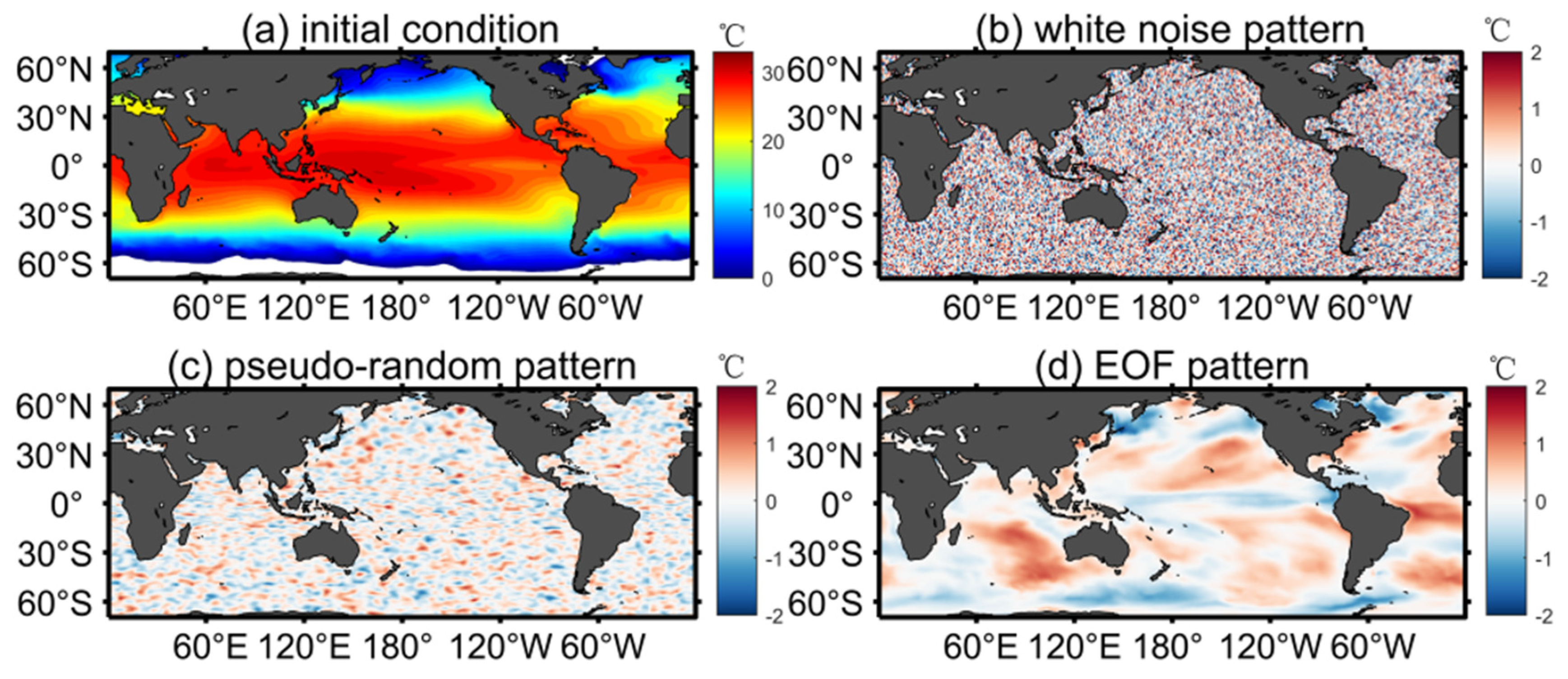
2.2. Initial Perturbation Methods

In this experiment, the initial state for the data assimilation is perturbed with different noises, which are described as follows. For simplicity, only the potential temperature for the upper 10 layers (about 100 m) is perturbed with 3 dimensional noises.

2.2.1. White Noise Pattern

The white noise perturbation method can be applied to construct the initial ensembles for the climate model. This method is to add a very small perturbation in the initial field, which not only guarantees the dynamic relationship between different variables in the model, but also avoids the model’s inadaptability to the initial perturbation. Particularly, the temperature of the mixed layer is slightly perturbed as follows
T i , j , k p e r t = ( 1 + α β i , j , k ) T i , j , k i n i t
where α is the amplitude with an order of 10 3 , β is a random number evenly distributed between (−1,1), and different random numbers are adopted for different samples. Subscripts i , j , and k are the spatial grid numbers, and superscripts p e r t and i n i t represent physical variables after and before the perturbation, respectively.

2.2.2. Pseudo-Random Pattern

Evensen [36] presented the procedure for generating pseudo random fields in Appendix E. Smooth pseudo random fields with mean values equal to zero, variance equal to one, and a specified covariance can be computed according to the algorithm involving the fast Fourier transform (FFT). Some parameters are used to create an ensemble of two-dimensional pseudo random fields with variance 1 and covariance determined by the decorrelation length. If the two-dimensional pseudo-random fields such as w k (k = 1,2…,N) are generated with a horizontal decorrelation length r h . It can be used to generate a three-dimensional field q with the following equation:
q k = α q k 1 + 1 α 2 w k 1
where q k indicates the kth layer of q , and q 1 = w 1 . The coefficient α [ 0 , 1 ] determines the vertical decorrelation of the initial field.
In this work, the perturbation fields are firstly generated to 1° grids and then interpolated into the POP grid where the decorrelation length is about 6 degrees in longitude for each field. And then, the coefficient α = e 0.1 is used to generate a three-dimensional field in which the temperature in the upper 10 layers is perturbed.

2.2.3. EOF Pattern

According to Hoteit et al. [48], a second-order sampling scheme [49] is used to generate the initial ensemble. Firstly, the 30-years free run without data assimilation is used to represent the variability of the model states. Secondly, an Empirical Orthogonal Function (EOF) analysis is applied to extract the dominant variability from the long period model trajectory. Then, the initial states are generated using the following equation,
x 0 i = x ¯ + N L 0 σ i T
where N is the ensemble size, L 0 is the matrix whose N 1 columns are the EOFs, x ¯ is the mean of the long-term trajectory, and σ i is the i th of a ( N 1 ) × N random matrix with orthonormal columns and zero column sums.
Figure 1b–d shows the spatial pattern of these perturbations, which describe and propagate the uncertainty of the estimate state. It can be seen that Figure 1b has no spatial correlation because it is generated by white noise. Figure 1c is smoother and has a clear spatial correlation, whereas Figure 1d shows its mode because it contains the main variability from the 30 years CESM (POP) data.

2.3. Analysis of Variance

Analysis of variance, also known as “F-test”, is used to test the significance of two or more groups with different means [50]. The idea is that the total variation in all data is equal to the between-group variation plus the within-group variation.
For a matrix k × n , where k denotes the number of groups and n denotes the number of data in each group, then the off-mean-sum-of-squares of the total variation ( S S t o t a l ) is first calculated, that is, the sum of squares of the differences between all data and the total mean ( X ¯ ¯ ).
X ¯ ¯ = i = 1 k j = 1 n X i , j n i
S S t o t a l = i = 1 k j = 1 n ( X i , j X ¯ ¯ ) 2
X ¯ i = j = 1 n X i , j n i
S S w i t h i n = i = 1 k j = 1 n ( X i , j X ¯ i ) 2
M S w i t h i n = S S w i t h i n n k
S S b e t w e e n = i = 1 k n i ( X ¯ i X ¯ ¯ ) 2
M S b e t w e e n = S S b e t w e e n k 1
F = M S b e t w e e n M S w i t h i n
where X i , j is the j th data of the i th group. X ¯ i is the mean of group i , S S w i t h i n is the within-group variance, i.e., the variance of group, S S b e t w e e n is the between-group variance, M S is the mean squared error, and F is the F-statistics which is the ratio of the mean squared error. In addition, it can also be calculated as follows.
S S t o t a l = S S w i t h i n + S S b e t w e e n
Analysis of variance compares the means of several groups to test the hypothesis that they are all equal, and sometimes this alternative may be too general. The work may need information about which pairs of means are significantly different, and which are not. A multiple comparison test (MCT) can provide this information [51]. The t-test is not appropriate for MCT, and the commonly used method is the SNK (Student–Newman–Keuls) method, also known as the q-test.

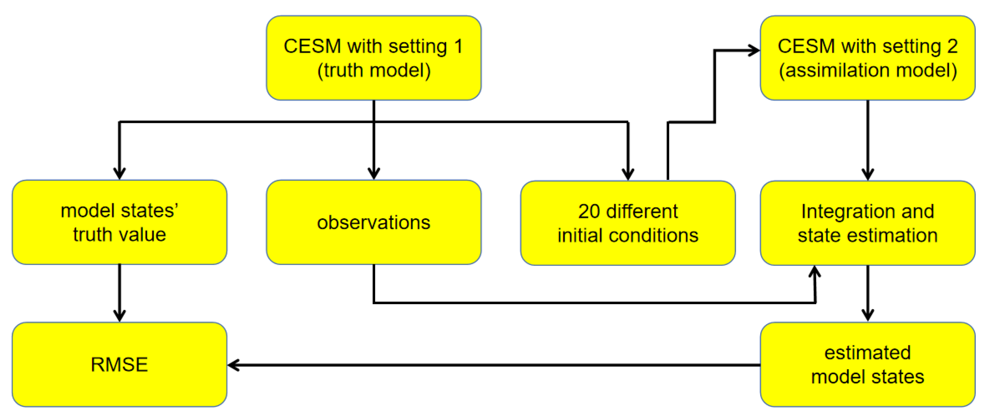
2.4. Experiment Design

2.4.1. Design of Observation

Coupled data assimilation (CDA) is a multitask problem that involves many issues: coupled model bias, sampling of the observing system, validation of the analysis scheme, etc. [24] A CDA system is complicated since any uncertainty in the aspects described above may cause the evaluation of CDA results to become extremely difficult. To reduce the complexity, this study excludes the model bias issue by using the Observation System Simulation Experiment (OSSE). The approach is to experiment with simulated data as “observations” that need to be assimilated. The Figure 2 displays a schematic diagram of the assimilation process. The data obtained from model setting 1 are used as “truth”, then, observational errors (a white noise with a standard deviation of 0.25 °C) are added to the “truth” as the observations which are assimilated into model setting 2. Then it is feasible to evaluate the assimilation quality by verifying assimilation results against the “truth”, so that any up/downgrade of the assimilation system, when a new assimilation component or observational data type is added, or when an assimilation parameter is tuned, can be quantified.

2.4.2. Design of Assimilation Experiments

The patterns of perturbations that would be added to the initial conditions are described in Section 2.2. There are also two strategies to generate the initial ensemble. One is to add the perturbations directly to the initial conditions, whereas the second strategy first perturbs the initial conditions with small amplitude and then integrates the model for one year. After a period of adjustment, it can ensure the ensemble spread grows sufficiently while the dynamic balance of model variables is preserved. It is noteworthy that the white-noise perturbation is not added directly in the experiment, since the random perturbation fields without a spin-up period are not well in dynamic balance to integrate the model. Therefore, five perturbation strategies are compared in this experiment, as listed in Table 2. In this experiment, only the potential temperature of the model states in the mixed layers of ocean are perturbed. All the data assimilation simulations are run for two years and the SST observations are assimilated every five days.

3. Results

3.1. The Initial Uncertainties and Ensemble Spread

The initial ensembles play an important role in data assimilation. The initial ensembles generated from the above procedure should be examined before running data assimilation with them. In this section, we first examine their spreads and check if they can present the actual uncertainties that can be estimated using model minus observations. Since only the SST was assimilated, we concentrate on the error statistics of the SST in this paper. Figure 3a depicts the SST errors of the initial guess against observation and Figure 3b–f shows the ensemble spreads (standard deviations) of the initial ensembles. SST errors are greatest in the East Equatorial Pacific, with about 1.6 to 1.8 °C. The values of the ensemble spread in the five experiments are of comparable amplitude. With the exception of EvensenT experiment (Figure 3b), the spreads of other initial ensembles have similar patterns as the model errors and all overestimate the value of ensemble spread in the mid and high latitudes. It is clear that the SSTs in mid and high latitudes are most sensitive to small-scale perturbations. This indicates that the background error covariance in these regions is probably triggered by small-scale physical processes, while the Equatorial region is more sensitive to perturbations of the ENSO mode. The effect of this irrational spread on the field of assimilation analysis is further investigated, as follows.

3.2. Assessing Differences between Assimilation Experiments

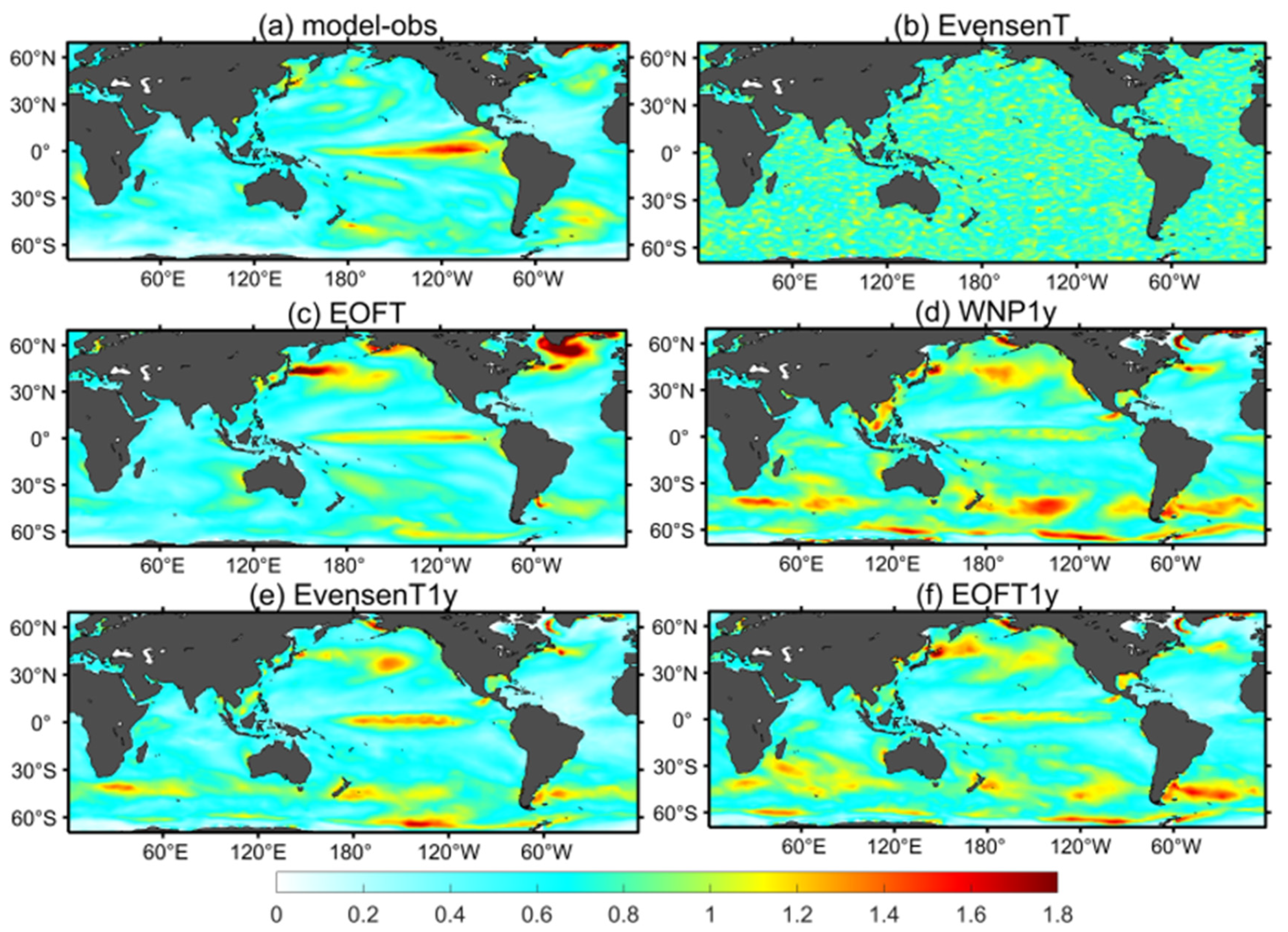
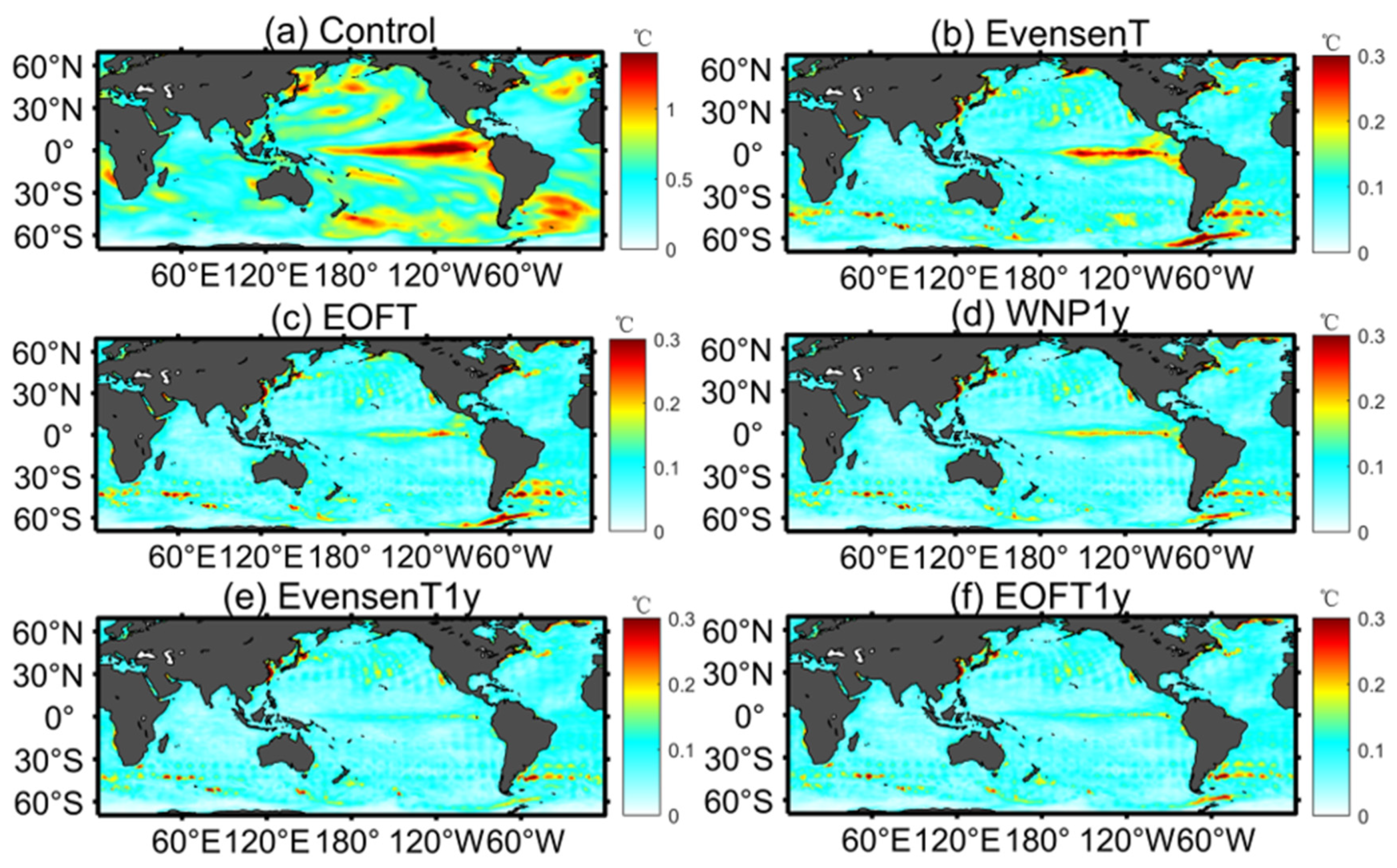
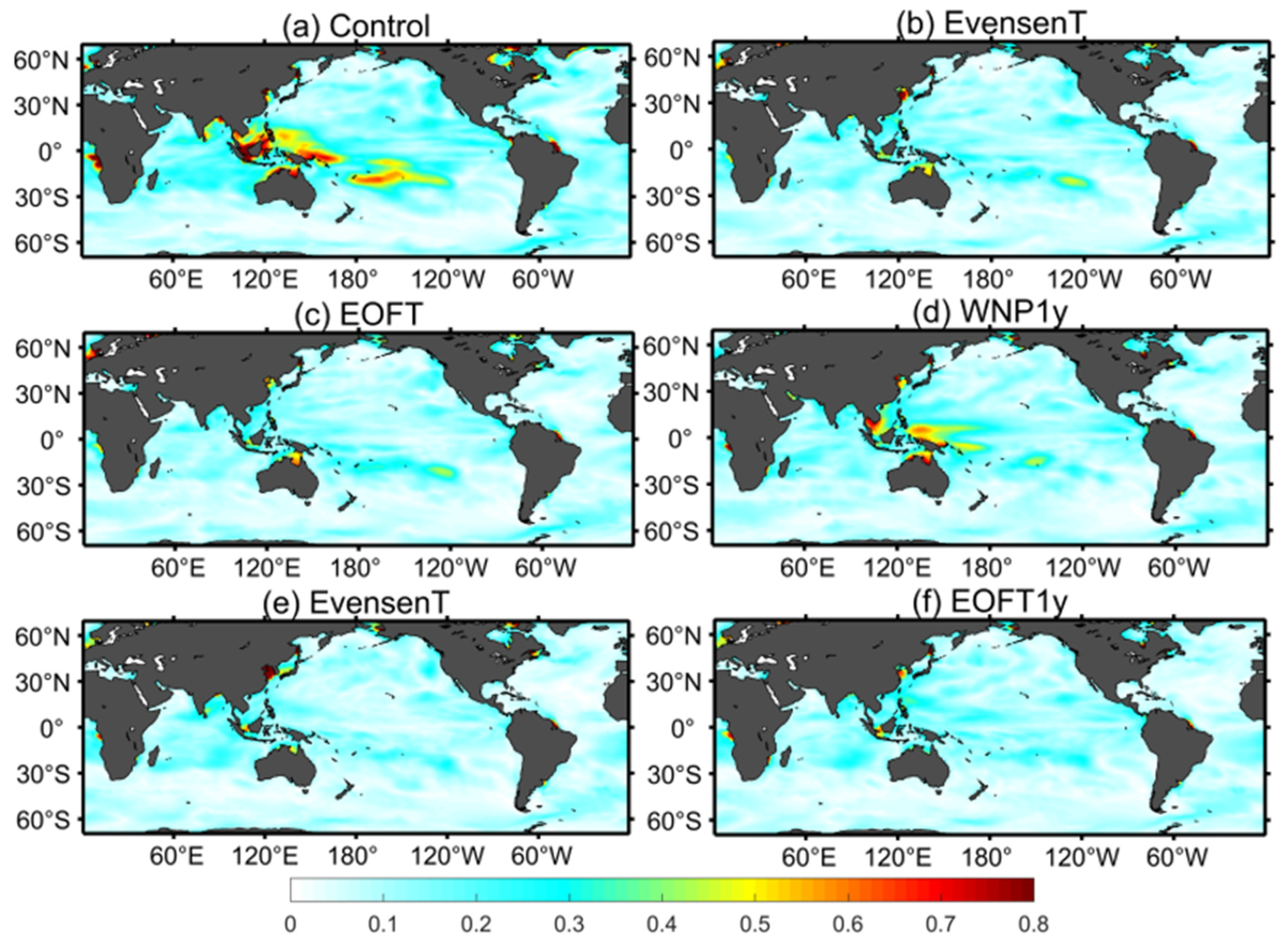
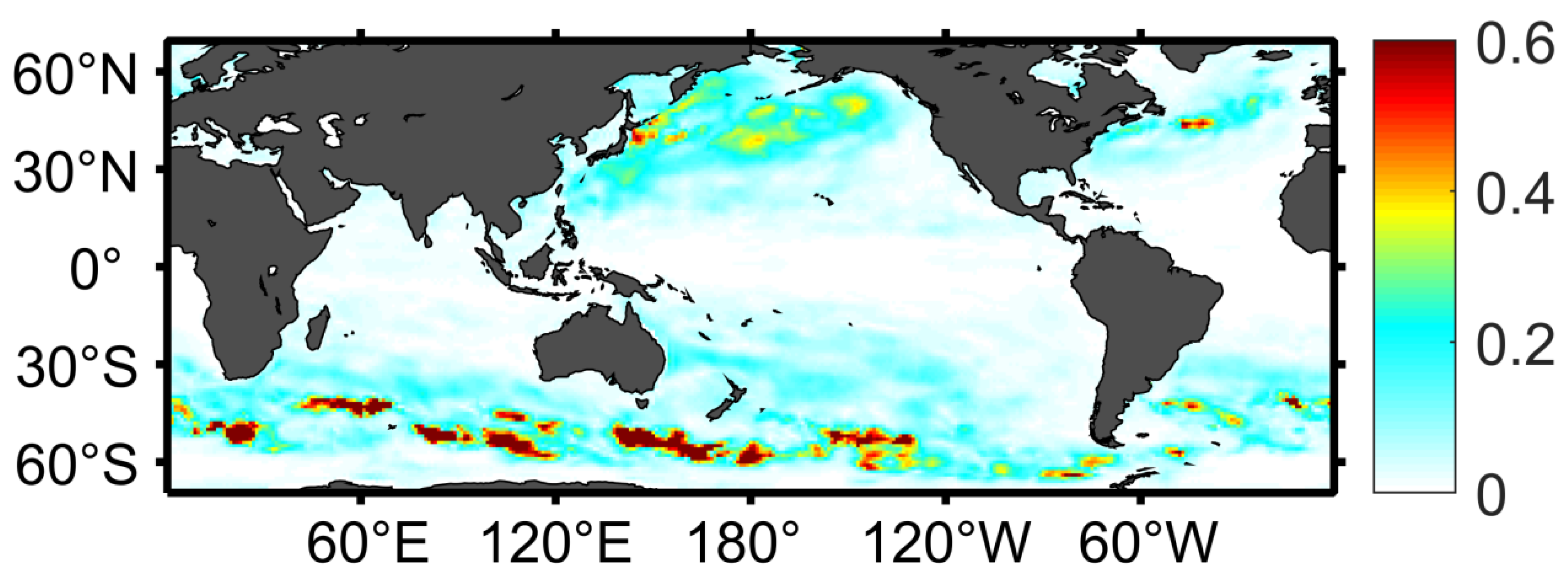
3.2.1. Spatial Distributions
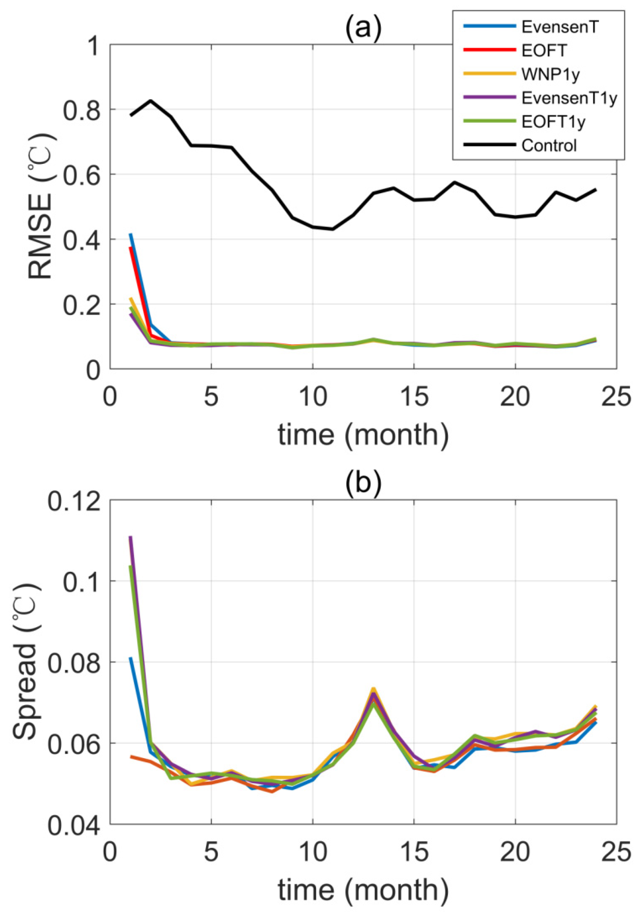
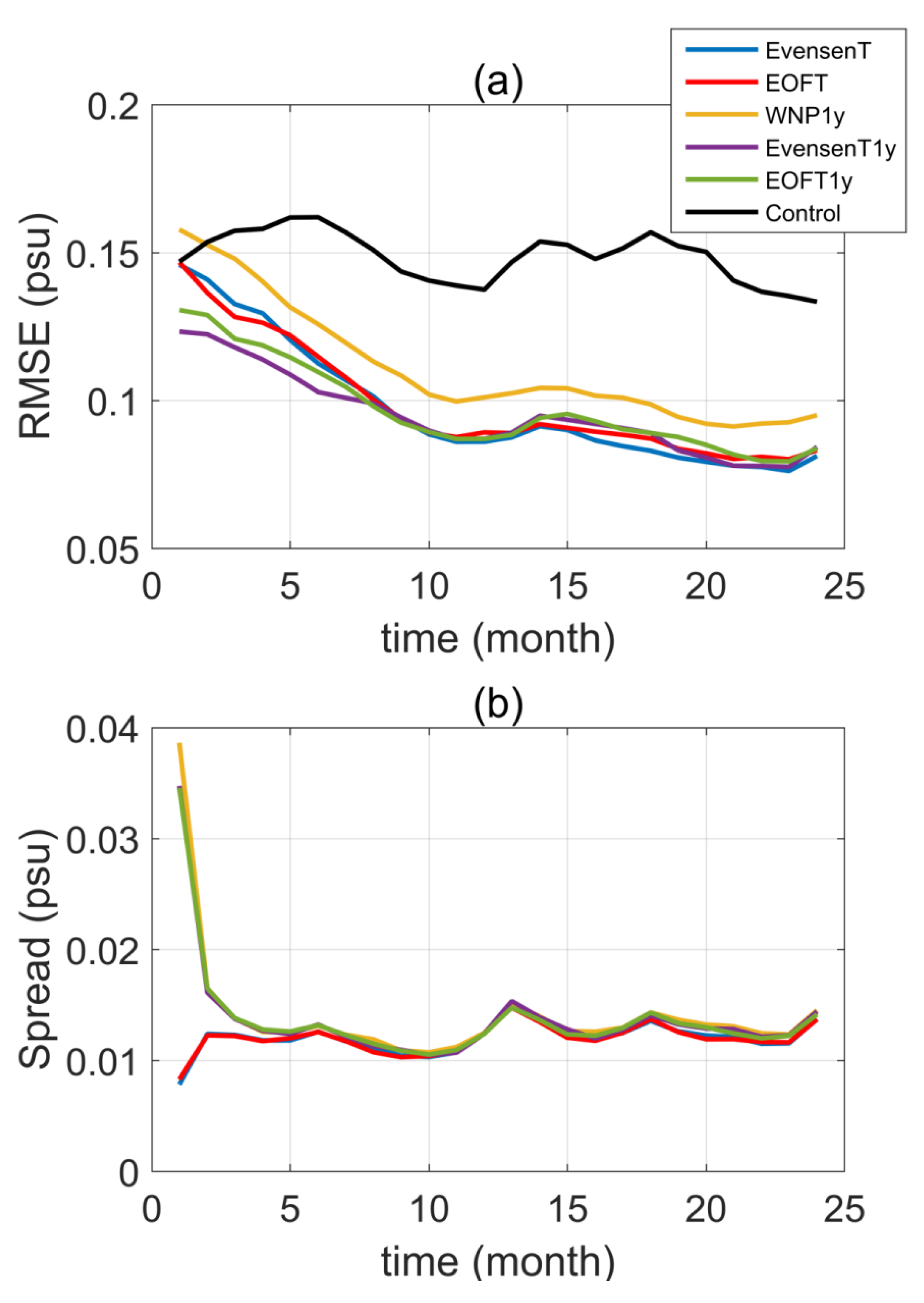
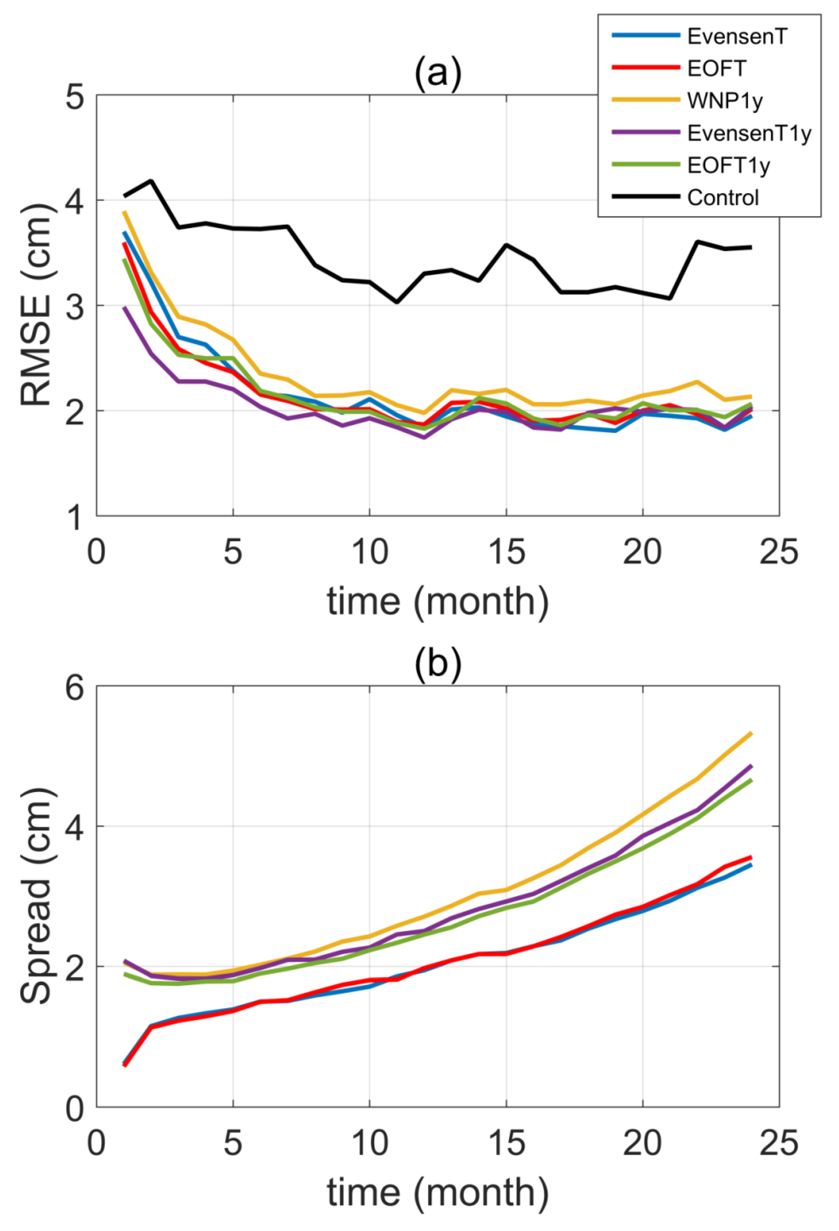
The results of the 24-month mean spatial distribution of RMSE from the various experiments are displayed in Figure 4. In addition, to avoid interfering with high latitude inaccuracies due to the model and observation deficiency, the region between 70° S and 70° N is evaluated in this work. Figure 4a is the same as Figure 3a, except that the color bar has been changed to show the effect of assimilation. It can be seen that the model’s simulations of SST in the Kuroshio Extension, tropical eastern Pacific, and high latitude in the southern Pacific and southwest of the Atlantic have considerable bias, with the maximum value exceeding 1.4 °C. In comparison to the control experiment (Figure 4a), the assimilation experiments (Figure 4b–f) show that the simulation of SST improves significantly. However, some small differences can be found in the results of the assimilation experiments, for example, the errors of the EvensenT experiment are the largest in the Eastern Equatorial Pacific, about 0.3 °C, but other experiments can even reach 0.1 °C. This is due to the fact that the perturbation of the EvensenT experiment is a pseudo-random pattern, as also mentioned in the previous chapter, which makes the standard deviation of its SST not reasonably distributed in the Eastern Equatorial Pacific (Figure 3b). Then, in the early stage of assimilation, the SST error will certainly be larger than the SST error of other experiments; therefore, such a result will be obtained after time averaging. In addition, SST assimilation improves not only areas with high bias, but also areas with low bias, such as the Indian Ocean.
Although only the SST was assimilated, the results of other variables, such as sea surface salinity, also need to be examined. Figure 5 shows the comparison between assimilation experiments and control experiments in terms of sea surface salinity (SSS) errors. As seen in the control experiment (Figure 5a), the sea surface salinity errors in the model are mainly distributed in the western Pacific warm pool and extend to the southeastern seas, where they are as high as 0.8 psu. Such large errors also occur in the nearshore region, from uncertainties in runoff simulations, and in the high-latitude polar region, from uncertainties in sea ice simulations, but both are due to uncertainties in freshwater fluxes that lead to large SSS errors. After assimilation, the simulation of SSS improves noticeably in these areas. While the simulation of SSS has improved significantly, results of SSS demonstrate that the differences between the various assimilation experiments have begun to emerge. It is clear that in the white noise experiment (Figure 5d), there are still significant SSS errors in the western Pacific warm pool, with values close to the model error, both about 0.4 psu. The improvement effect is obviously not as strong as in the other assimilation experiments, which were able to reduce the SSS error to 0.1 psu in the western Pacific warm pool.
In addition, the sea surface height is also an important variable. Figure 6 shows the comparison between assimilation experiments and control experiments in terms of sea surface height (SSH) errors. The simulation of SSH is also greatly improved. As demonstrated by the control experiment (Figure 6a), the model is biased toward low latitudes in the Pacific, near the equator in the Indian Ocean, and the high latitude region in North Atlantic, reaching up to 12 cm. However, the error in SSH can be reduced to about 2 cm after assimilation of SST. Although there is a significant improvement in these areas after assimilation, the SSH error in the westerlies in the Southern Ocean is not much reduced, and here, the covariance between SSH and SST is more influenced by small-scale physical processes. The results of SSH also indicate that the discrepancies between various assimilation experiments have begun to emerge. It can be found that the initial ensemble of the experiment is adjusted by the model integration, then, the SSH error in the Kuroshio Extension (Japan’s East coast) will grow rapidly, and its value even exceeds the error of the model (3~4 cm). When comparing the white noise experiment to other assimilation experiments, it is also clear there is still a significant SSH simulation bias in the north of the equatorial Pacific in the white noise experiment (Figure 6d), and the improvement is obviously not as good as other assimilation experiments.

3.2.2. Time Series

In addition to examining the performance of assimilation, it is also important to test the time evolution of the RMSE of the variables. Figure 7 illustrates the results of time series of the ensemble root mean square error (RMSE) of variables such as SST, SSS, and SSH. According to the results of SST (Figure 7a), the assimilation experiment’s RMSE is much more reduced than that of the control experiment. The differences between assimilation experiments are primarily due to assimilation prior to achieving stability. Approximately three months after assimilation, all assimilation experiments’ RMSE have decreased to a steady-state, and the assimilation method has achieved convergent solution, with the global average RMSE decreasing to 0.08 °C. It is obvious that the rates of decline for various experiments vary. As demonstrated by the spread of SST (Figure 7b), all assimilation experiments can achieve a steady state. Furthermore, the magnitude of this steady state value is comparable to the RMSE, which is fairly reasonable.
Then, based on the results of SSS (Figure 8a), it is clear that the SSS and SST conclusions are considerably dissimilar. However, the assimilation experiments’ RMSE are much smaller than that of the control experiment. In contrast to the preceding experiment, the RMSE of the assimilation experiment decreases, but not as rapidly as the result of SST. The experiments do not achieve apparent stability after two years. Additionally, there are discrepancies among assimilation experiments, with one experiment (WNP1y) exhibiting much larger bias than others over a two-year period. This is achieved by integrating the model after adding white noise perturbation to the initial state. SSS has a similar distribution to SST (Figure 8b). The spread of SSS in the initial ensemble is adjusted to the steady-state via assimilation, but the spread of SSS is much smaller than its RMSE, indicating that the covariance between SST and SSS in assimilation cannot effectively adjust SSS and the change in SSS is due to the constraint in CESM.
The SSH result is shown in following figure (Figure 9a). The assimilation experiments’ RMSE is also much less than that of the control experiment, however, SSH’s result is not as close to a critical value as those of SST. Therefore, while the assimilation can improve the simulation of SSS and SSH, it cannot induce a steady state in any physical variable except SST in a short time. However, the RMSE of the WNP1y assimilation experiment is larger than that of other assimilation experiments. It is discovered in the previous spatial distribution that the white noise experiments result in much greater RMSEs in SSS and SSH than other experiments. The spread of SSH (Figure 9b) shows that the five experiments are clearly split into two groups. One is integrated by the model and the other is not, i.e., the spread of SSH begins at zero and continues to increase in all assimilation experiments. While it does not achieve a steady state, its magnitude is close to the RMSE, demonstrating that covariance between SST and SSH during assimilation can effectively adjust SSH.

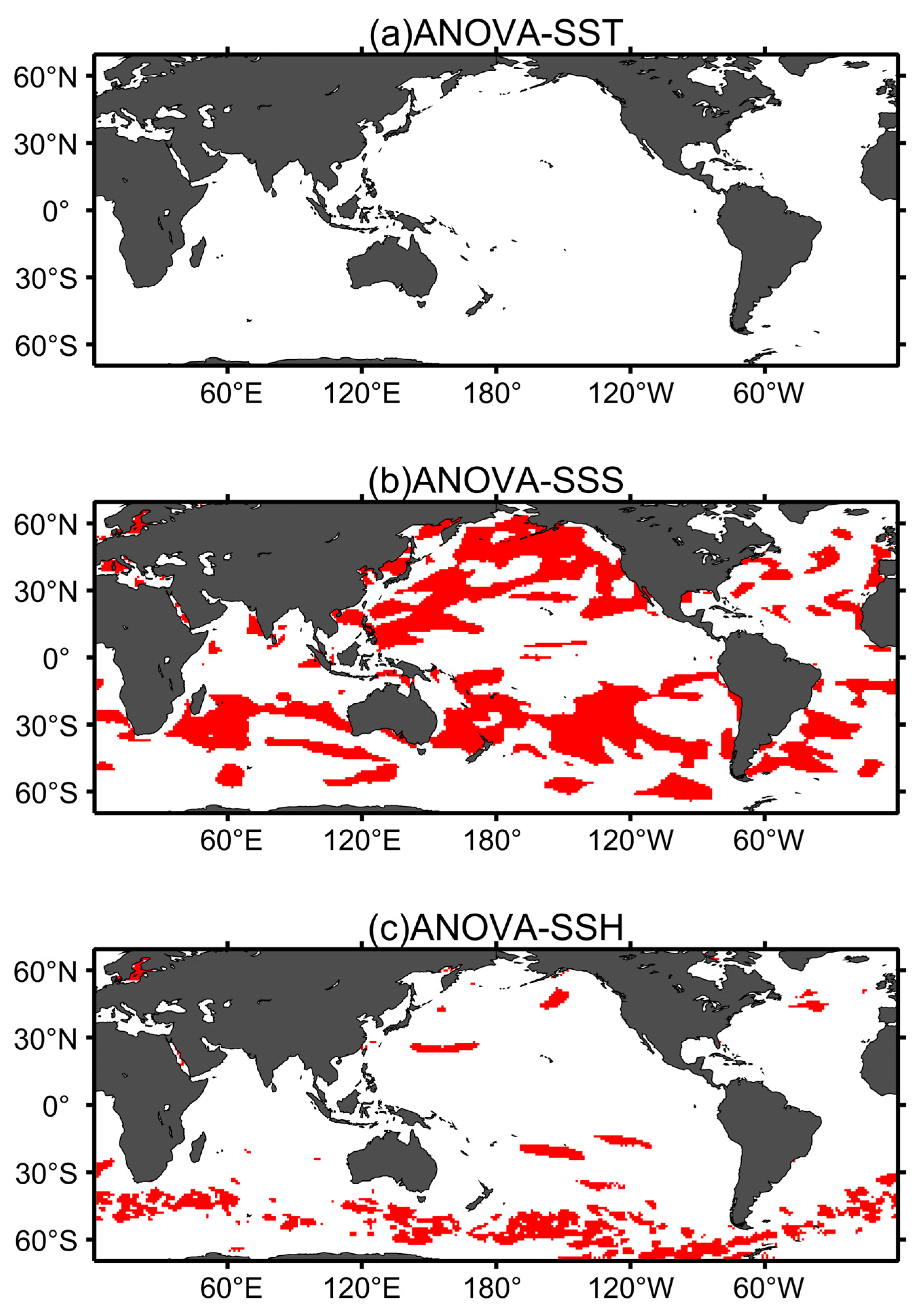
3.2.3. Significance Test

Are the differences between these five assimilation experiments significant in terms of SSS and SSH results? ANOVA is used to examine the time series of RMSE of the five assimilation experiments, that is, the sequence of five groups of numbers, in order to calculate the P-value. If the P-value is more than 0.05, it indicates that no significant difference exists between the various experiments. As shown in Table 3, there is no significant difference between assimilation experiments for SST; the P-value is significantly more than 0.05, which indicates the consequence of assimilating solely SST data. However, the P-value is smaller than 0.05 for SSS and SSH. The spatial distribution (Figure 5b–f, Figure 6b–f) demonstrates which areas exhibit these disparities. In the western Pacific warm pool, the SSS is drastically different, whereas in the northern equatorial Pacific and Kuroshio Extension, the SSH is drastically different.
Although the ANOVA results indicate a highly significant difference in the assimilation of distinct experimental simulations of SSS and SSH, this does not mean that any two assimilation experiments have highly significant differences. The MCT is used to examine significance between each of the two experiments, as results show in Table 4. All P-values are clearly lower when compared to the third assimilation experiment (WNP1y). This demonstrates that the third assimilation experiment is quantitatively distinct from others. The time series of the four assimilation experiments without the WNP1y is then analyzed using ANOVA. SSS and SSH have P-Values of 0.8606 and 0.5183, respectively, which are much greater than 0.05. This indicates that the initial ensemble of the third assimilation experiment has the poorest assimilation impact and is significantly different from the other assimilation experiments, while the other assimilation experiments show little difference of significance.
The ANOVA is used to analyze individual points to see which regions exhibit significant changes in the SST, SSS, and SSH simulations, except for WNP1y. For SST (Figure 10a), the result is perfect, with no discernible change in the horizontal distribution of SST among the four groups of assimilation experiments. However, there is no evident pattern for SSS (Figure 10b). Due to the small spread of SSS in the preceding study, EAKF does not successfully modify SSS via the covariance between SSS and SST, but instead via the physical relationship in CESM. SSH (Figure 10c) exhibits a distinct pattern. In other words, the region where the assimilation experiments differ is mostly the area surrounding the Antarctic Circumpolar Current (ACC). As previously discussed, the spread of SSH in the assimilation experiment is normal, and because the covariance can be used to alter SSH, this covariance pattern can be linked to the ANOVA pattern.
EAKF estimates the covariance between a component of a particular state variable and observation variables as the increment for that component. Covariance is a critical aspect in determining the magnitude of increments. Of course, it is not the region with high covariance that accounts for the significant difference in the simulations of the four assimilation experiments, but the difference in the covariance between SST and SSH for each assimilation experiment, which is equivalent to analyzing the spread of the covariance. As a result, prior to conducting CESM-EAKF, it is important to determine the horizontal distribution of covariance between SSH and SST. As illustrated in Figure 11, the spread of covariance between SSH and SST is greater in the Antarctic Circumpolar Current area during assimilation; this region exhibits one of the largest differences in SSH in the EAKF update. This also explains why there is a pattern of SSH in Figure 10 by ANOVA, and it demonstrates that the covariance correction in assimilation has a noticeable effect on SSH.

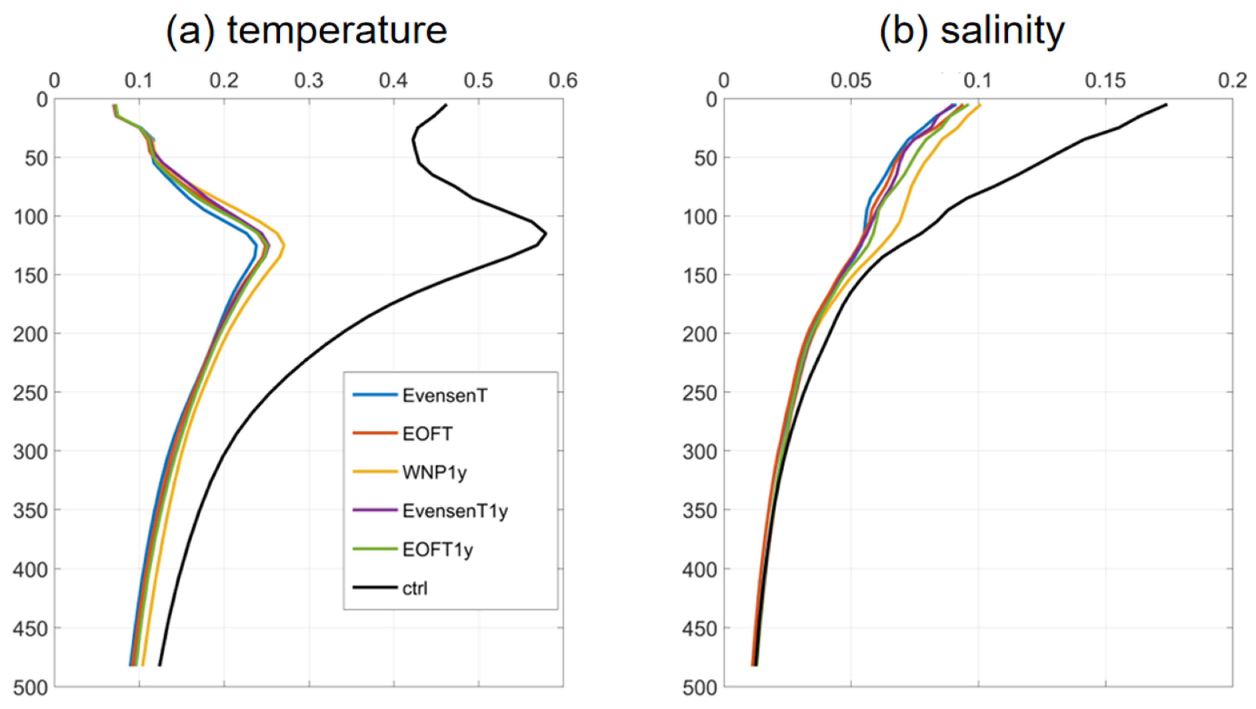
3.2.4. Vertical Distribution

SST observations provide sea surface information. Therefore, it is natural that the assimilation process improves the modeled SST or other variables of the sea surface. Whether or not the subsurface thermohaline structure is improved is investigated in this section.
Figure 12a,b shows vertical profiles of the RMSEs of global temperature and salinity, respectively. All assimilation experiments improve the temperature simulation in the upper 500 m, with the best improvement in the mixed layer, which is reduced by about 0.4 °C. This is because the assimilation data is SST, which improves only the physical characteristics in the mixed layer. With increasing depth, the RMSE of all experiments approaches zero. As with time series analysis, all experiments are quite similar to the SST simulation and have the same effect. The largest errors are in the thermocline, about 0.25 °C, which is attributed to the substantial error in the model’s original simulation of thermocline. After all, the ocean incorporates intricate physical processes such as subsurface entrainment, which makes it difficult for models to simulate it. Additionally, the vertical distribution of temperature RMSE indicates that the WNP1y assimilation experiment has a little larger RMSE than other assimilation experiments below the surface.
Although the salinity improvement is most pronounced in the surface layer, with a decrease of 0.095 psu, the error is still the largest over the entire profile, at about 0.09 psu. This is because the surface salinity is poorly constrained and impact of erroneous fresh-water fluxes and ocean mixing manifests itself in errors in the salinity field. The improvement in salinity by data assimilation is more robust in the mixed layer. This improvement is not only due to the direct assimilation of SST observations, but also to the balance relations between temperature and salinity. As previously observed, the vertical profiles of salinity bias indicate that the WNP1y assimilation experiment has a greater RMSE than other assimilation experiments in the upper 300 m.

4. Discussion

This work only provides an insight on the issue of the generation of the initial ensemble, especially for the data assimilation of complex CGCMs. Nevertheless, there are still some areas that deserve more attention and need further improvement.
This work is made on the foundation of the OSSE with the perfect model assumption. However, it is much more complicated in real data assimilations. The observation error added to the “truth” is quite coarse and is just a white noise. However, the actual observation error has a more complex distribution in both space and time. In the ensemble assimilation, both the observation error and the model error greatly affect the increment of the variables. In addition, many other factors such as the feasibility, computational burdens, and efficiency should be taken into consideration, which we will pursue in our future work.
Improving the performance of the assimilation system by continuously improving the initial ensemble is also beneficial for high-resolution numerical simulations. In particular, in this work, the assimilated variable is the SST, and the SST data are advantageous as an observation with small observation error and large data volume. This can make the simulated SST more accurate and can also help us to better understand some physical processes affected by SST [52,53].

5. Conclusions

In this work, we have compared different perturbation strategies of the initial ensemble for ocean data assimilation in a fully coupled earth system model (the NCAR/CESM). The data assimilation system is already established with an open-source community tool, DART. We have designed the twin experiments with the observation system simulation experiment framework, in which the observations are simulated and assimilated to the model with perturbed initial ensembles to investigate the influence of initial perturbations.
Three perturbation patterns, white noises, pseudo-random fields, and EOF patterns, are considered and combined with various integration strategies. In total, five perturbation strategies are compared with the OSSE. The following conclusions are made accordingly.
For the observed variables (SST), experiments with perturbations added directly to the initial conditions will necessarily lead to larger errors at the beginning than those adjusted by model integration. However, its convergence will also be faster than the latter. Therefore, regardless of the strategy used to create the initial ensemble, all experiments have a nearly identical effect after three or four months.
For adjusted variables (SSS and SSH), it is discovered that RMSE in horizontal distribution, time series, and vertical distribution of one assimilation experiment is significantly greater than that of other experiments, namely, the experiment of adding small-scale white noise perturbation and integrating the model for one year (WNP1y). This indicates that although there is a model integral to help adjust the spread of the other variables, the added perturbation is white noise, which results in a distribution of spread that does not properly represent the error statistics of the model states. This is critical for development of reanalysis data and Ensemble Prediction, as it is vital to avoid an initial ensemble with a large RMSE.
The significance of difference between five assimilation experiments is also examined. It indicates that the differences in observed variables (SST) are not significant, however, differences in adjusted variables (SSS and SSH, etc.) are significant, which are attributed to the WNP1y experiment. In different areas, the significance of difference for the four strategies varies. Results of SST (assimilated variable) are ideal; global differences are not significant. The SSS (adjusted variable) result is opposite, and no discernible pattern exists. By analyzing the spread of covariance, it is demonstrated that result of SSS is not optimal, primarily because the spread is much smaller than the RMSE, implying the covariance correction has no effect on SSS. The result of SSH (adjusted variable) is acceptable, owing to a large difference in the Antarctic Circumpolar Current.

Author Contributions

Conceptualization, Z.S. and S.D.; methodology, Z.S. and S.D.; validation, Z.S., S.D. and S.C.; formal analysis, S.D.; investigation, Z.S. and S.D.; data curation, S.D.; writing—original draft preparation, S.D.; writing—review and editing, Z.S., S.C. and R.W.; visualization, S.D.; supervision, Z.S. and S.C.; project administration, Z.S. and S.C.; funding acquisition, Z.S. and S.C. All authors have read and agreed to the published version of the manuscript.

Funding

This research was funded by the Shenzhen University Sustainable Support Plan under grant number WDZC20200819105831001, the Shenzhen Peacock Plan under grant number KQJSCX20170720174016789, the Fundamental Research Funds for the Central Universities under grant number B210201022, and the National Natural Science Foundation of China under grant number 42176003 and 41690124. Shengli is supported by the Scientific Research Start-up Funds (QD2021021C).

Institutional Review Board Statement

Not applicable.

Informed Consent Statement

Not applicable.

Data Availability Statement

The data presented in this study are available on request from the first author.

Acknowledgments

Many thanks to Youmin Tang for his advice on this study and for providing high performance computing resources.

Conflicts of Interest

The authors declare no conflict of interest.

References

  1. LeDimet, F.X.; Talagrand, O. Variational algorithms for analysis and assimilation of meteorological observations: Theoretical aspects. Tellus A Dyn. Meteorol. Oceanogr. 1986, 38, 97–110. [Google Scholar] [CrossRef]
  2. Derber, J.C. Variational four-dimensional analysis using quasi-geostrophic constraints. Mon. Weather Rev. 1987, 115, 998–1008. [Google Scholar] [CrossRef] [Green Version]
  3. Talagrand, O.; Courtier, P. Variational assimilation of meteorological observations with the adjoint vorticity equation. Part I: Theory. Q. J. R. Meteorol. Soc. 1987, 113, 1311–1328. [Google Scholar] [CrossRef]
  4. Courtier, P.; Thepaut, J.N.; Hollingsworth, A. A strategy for operational implementation of 4D-Var, using an incremental approach. Q. J. R. Meteorol. Soc. 1994, 120, 1367–1388. [Google Scholar] [CrossRef]
  5. Peng, S.Q.; Xie, L.A. Effect of determining initial conditions by four-dimensional variational data assimilation on storm surge forecasting. Ocean Model. 2006, 14, 1–18. [Google Scholar] [CrossRef] [Green Version]
  6. Huang, X.-Y.; Xiao, Q.; Barker, D.; Zhang, X.; Michalakes, J.; Huang, W.; Henderson, T.; Bray, J.; Chen, Y.; Ma, Z.; et al. Four-Dimensional Variational Data Assimilation for WRF: Formulation and Preliminary Results. Mon. Weather Rev. 2009, 137, 299–314. [Google Scholar] [CrossRef] [Green Version]
  7. Kalnay, E.; Kanamitsu, M.; Kistler, R.; Collins, W.; Deaven, D.; Gandin, L.; Iredell, M.; Saha, S.; White, G.; Woollen, J.; et al. The NCEP/NCAR 40 -year reanalysis project. Bull. Am. Meteorol. Soc. 1996, 77, 437–471. [Google Scholar] [CrossRef] [Green Version]
  8. Behringer, D.; Ji, M.; Leetma, A. An improved coupled model for ENSO prediction and implications for ocean initialization. Part 1: The ocean data assimilation system. Mon. Weather Rev. 1998, 126, 1013–1021. [Google Scholar] [CrossRef]
  9. Mogensen, K.; Molteni, M.; Weaver, A. The NEMOVAR Ocean Data Assimilation System as implemented in the ECMWF Ocean Analysis System for System 4. In Technical Memorandum 668; ECMWF: Reading, UK, 2012. [Google Scholar]
  10. Zuo, H.; Balmaseda, M.; Mogensen, K. The new eddy-permitting ORAP5 ocean reanalysis: Description, evaluation and uncertainties in climate signals. Clim. Dyn. 2017, 49, 791–811. [Google Scholar] [CrossRef]
  11. Kalman, R.E. A new approach to linear filtering and prediction problems. J. Basic Eng. 1960, 82, 35–45. [Google Scholar] [CrossRef] [Green Version]
  12. Burgers, G.; van Leeuwen, P.J.; Evensen, G. Analysis scheme in the ensemble Kalman filter. Mon. Weather. Rev. 1998, 126, 1719–1724. [Google Scholar] [CrossRef]
  13. Evensen, G. Sequential data assimilation with a nonlinear quasi-geostrophic model using Monte Carlo methods to forecast error statistics. J. Geophys. Res. Ocean. 1994, 99, 10143–10162. [Google Scholar] [CrossRef]
  14. Martin, M.J.; Balmaseda, M.; Bertino, L.; Brasseur, P.; Brassington, G.; Cummings, J.; Oke, P.R. Status and future of data assimilation in operational oceanography. J. Oper. Oceanogr. 2015, 8, s28–s48. [Google Scholar] [CrossRef]
  15. Anderson, J.L. An ensemble adjustment Kalman filter for data assimilation. Mon. Weather Rev. 2001, 129, 2884–2903. [Google Scholar] [CrossRef] [Green Version]
  16. Anderson, J.L. A local least squares framework for ensemble filtering. Mon. Weather Rev. 2003, 131, 634–642. [Google Scholar] [CrossRef] [Green Version]
  17. Anderson, J.; Hoar, T.; Raeder, K.; Liu, H.; Collins, N.; Torn, R.; Avellano, A. The data assimilation research testbed: A community facility. Bull. Am. Meteorol. Soc. 2009, 90, 1283–1296. [Google Scholar] [CrossRef] [Green Version]
  18. Haugen, V.E.; Evensen, G. Assimilation of SLA and SST data into an OGCM for the Indian Ocean. Ocean Dyn. 2002, 52, 133–151. [Google Scholar] [CrossRef]
  19. Chen, D.; Zebiak, S.E.; Busalacchi, A.J. An improved procedure for El Nino forecasting: Implications for predictability. Science 1995, 269, 1699–1702. [Google Scholar] [CrossRef] [PubMed] [Green Version]
  20. Chen, D.; Cane, M.A.; Zebiak, S.E.; Kaplan, A. The impact of sea level data assimilation on the Lamont model prediction of the 1997/98 El Nino. Geophys. Res. Lett. 1998, 25, 2837–2840. [Google Scholar] [CrossRef]
  21. Ballabrera, P.J.; Busalacchi, A.J.; Murtugudde, R. Application of a reduced-order Kalman filter to initialize a coupled atmosphereocean model: Impact on the prediction of El Niño. J. Clim. 2000, 14, 1720–1737. [Google Scholar] [CrossRef] [Green Version]
  22. Zebiak, S.E.; Cane, M.A. A model El Nino-Southern oscillation. Mon. Weather Rev. 1987, 115, 2262–2278. [Google Scholar] [CrossRef] [Green Version]
  23. Zheng, F.; Zhu, J.; Zhang, R.H.; Zhou, G. Improved ENSO forecasts by assimilating sea surface temperature observations into an intermediate coupled model. Adv. Atmos. Sci. 2006, 23, 615–624. [Google Scholar] [CrossRef]
  24. Zhang, S.; Harrison, M.; Rosati, A.; Wittenberg, A. System design and evaluation of coupled ensemble data assimilation for global oceanic climate studies. Mon. Weather Rev. 2007, 135, 3541–3564. [Google Scholar] [CrossRef] [Green Version]
  25. Zhang, S.; Rosati, A.; Harrison, M. Detection of multidecadal oceanic variability by ocean data assimilation in the context of a “perfect” coupled model. J. Geophys. Res. Ocean. 2009, 114, C12. [Google Scholar] [CrossRef] [Green Version]
  26. Zhang, S.; Rosati, A. An inflated ensemble filter for ocean data assimilation with a biased coupled GCM. Mon. Weather Rev. 2010, 138, 3905–3931. [Google Scholar] [CrossRef]
  27. Delworth, T.; Broccoli, A.; Rosati, A.; Stouffer, R.J.; Balaji, V.; Beesley, J.A.; Cooke, W.F.; Dixon, K.; Dunne, J.; Dunne, K.A.; et al. GFDL’s CM2 Global Coupled Climate Models. Part I: Formulation and Simulation Characteristics. J. Clim. 2006, 19, 643–674. [Google Scholar] [CrossRef]
  28. Yin, X.; Qiao, F.; Shu, Q. Using ensemble adjustment Kalman filter to assimilate Argo profiles in a global OGCM. Ocean Dyn. 2011, 61, 1017–1031. [Google Scholar] [CrossRef] [Green Version]
  29. Karspeck, A.R.; Danabasoglu, G.; Anderson, J.; Karol, S.; Collins, N.; Vertenstein, M.; Raeder, K.; Hoar, T.; Neale, R.; Edwards, J. A global coupled ensemble data assimilation system using the Community Earth System Model and the Data Assimilation Research Testbed. Q. J. R. Meteorol. Soc. 2018, 144, 2404–2430. [Google Scholar] [CrossRef]
  30. Karspeck, A.R.; Yeager, S.; Danabasoglu, G. An ensemble adjustment kalman filter for the CCSM4 ocean component. J. Clim. 2013, 26, 7392–7413. [Google Scholar] [CrossRef] [Green Version]
  31. Raeder, K.; Anderson, J.L.; Collins, N.; Hoar, T.J.; Kay, J.E.; Lauritzen, P.H.; Pincus, R. DART/CAM: An ensemble data assimilation system for CESM atmospheric models. J. Clim. 2012, 25, 6304–6317. [Google Scholar] [CrossRef]
  32. Zhang, Y.F.; Hoar, T.; Yang, Z.L.; Anderson, J.; Toure, A.; Rodell, M. Assimilation of MODIS snow cover through the Data Assimilation Research Testbed and the Community Land Model version 4. J. Geophys. Res. Atmos 2014, 119, 7091–7103. [Google Scholar] [CrossRef]
  33. Doucet, A.; De Freitas, N.; Gordon, N. An introduction to sequential Monte Carlo methods. In Sequential Monte Carlo Methods in Practice; Springer: Berlin/Heidelberg, Germany, 2001; pp. 3–14. [Google Scholar]
  34. Hoteit, I.; Pham, D.T.; Triantafyllou, G.; Korres, G. A new approximate solution of the optimal nonlinear filter for data assimilation in meteorology and oceanography. Mon. Weather Rev. 2008, 136, 317–334. [Google Scholar] [CrossRef]
  35. Wan, L.; Zhu, J.; Bertino, L.; Wang, H. Initial ensemble generation and validation for ocean data assimilation using HYCOM in the Pacific. Ocean Dyn. 2008, 58, 81–99. [Google Scholar] [CrossRef]
  36. Evensen, G. The ensemble Kalman filter: Theoretical formulation and practical implementation. Ocean Dyn. 2003, 53, 343–367. [Google Scholar] [CrossRef]
  37. Pham, D.T.; Verron, J.; Roubaud, M.C. A singular evolutive extended Kalman filter for data assimilation in oceanography. J. Mar. Syst. 1998, 16, 323–340. [Google Scholar] [CrossRef]
  38. Nerger, L.; Hiller, W.; Schröter, J. A comparison of error subspace Kalman filters. Tellus A Dyn. Meteorol. Oceanogr. 2005, 57, 715–735. [Google Scholar] [CrossRef]
  39. Hurrell, J.W.; Holland, M.M.; Gent, P.R.; Ghan, S.; Kay, J.E.; Kushner, P.J.; Lamarque, J.F.; Large, W.G.; Lawrence, D.; Lindsay, K.; et al. The Community Earth System Model: A framework for collaborative research. Bull. Am. Meteorol. Soc. 2013, 94, 1339–1360. [Google Scholar] [CrossRef]
  40. Yeager, S.; Karspeck, A.R.; Danabasoglu, G.; Tribbia, J.; Teng, H. A decadal prediction case study: Late 20th century North Atlantic Ocean heat content. J. Clim. 2012, 25, 5173–5189. [Google Scholar] [CrossRef]
  41. Meehl, G.; Goddard, L.; Boer, G.; Burgman, R.; Branstator, G.; Cassou, C.; Corti, S.; Danabasoglu, G.; Doblas-Reyes, F.; Hawkins, E.; et al. Decadal climate prediction: An update from the trenches. Bull. Am. Meteorol. Soc. 2014, 95, 243–267. [Google Scholar] [CrossRef] [Green Version]
  42. Karspeck, A.R.; Yeager, S.; Danabasoglu, G.; Teng, H. An evaluation of experimental decadal predictions using CCSM4. Clim. Dyn. 2015, 44, 907. [Google Scholar] [CrossRef]
  43. Neale, R.; Chen, C.C.; Gettelman, A.; Lauritzen, P.; Park, S.; Williamson, D.; Conley, A.; Garcia, R.; Kinnison, D.; Lamarque, J.F.; et al. Description of the NCAR Community Atmosphere Model (CAM 5.0). In Technical Note TN-486+STR; NCAR: Boulder, CO, USA, 2010. [Google Scholar]
  44. Danabasoglu, G.; Bates, S.; Briegleb, B.; Jayne, S.; Jochum, M.; Large, W.; Peacock, S.; Yeager, S. The CCSM4 ocean component. J. Clim. 2012, 25, 1361–1389. [Google Scholar] [CrossRef] [Green Version]
  45. Holland, M.; Bailey, D.; Briegleb, B.; Light, B.; Hunke, E. Improved sea ice shortwave radiation physics in CCSM4: The impact of melt ponds and aerosols on arctic sea ice. J. Clim. 2012, 25, 1413–1430. [Google Scholar] [CrossRef]
  46. Lawrence, D.; Oleson, K.; Flanner, M.; Thornton, P.; Swenson, S.; Lawrence, P.; Zeng, X.; Yang, Z.L.; Levis, S.; Sakaguchi, K.; et al. Parameterization improvements and functional and structural advances in version 4 of the Community Land Model. J. Adv. Modeling Earth Syst. 2011, 3, M03001. [Google Scholar] [CrossRef]
  47. Gaspari, G.; Cohn, S. Construction of correlation functions in two and three dimensions. Q. J. R. Meteorol. Soc. 1999, 125, 723–757. [Google Scholar] [CrossRef]
  48. Hoteit, I.; Hoar, T.; Gopalakrishnan, G.; Collins, N.; Anderson, J.; Cornuelle, B.; Köhl, A.; Heimbach, P. A MITgcm/DART ensemble analysis and prediction system with application to the Gulf of Mexico. Dyn. Atmos Ocean. 2013, 63, 1–23. [Google Scholar] [CrossRef]
  49. Pham, D.T. Stochastic methods for sequential data assimilation in strongly nonlinear systems. Mon. Weather Rev. 2001, 129, 1194–1207. [Google Scholar] [CrossRef]
  50. Hogg, R.; Ledolter, J. Engineering Statistics; MacMillan: New York, NY, USA, 1987. [Google Scholar]
  51. McHugh, M. Multiple comparison analysis testing in ANOVA. Biochem. Med. 2011, 21, 203–209. [Google Scholar] [CrossRef] [PubMed]
  52. Meroni, A.; Parodi, A.; Pasquero, C. Role of SST patterns on surface wind modulation of a heavy midlatitude precipitation event. J. Geophys. Res. Atmos 2018, 123, 9081–9096. [Google Scholar] [CrossRef]
  53. Ricchi, A.; Bonaldo, D.; Cioni, G.; Carniel, S.; Miglietta, M. Simulation of a flash-flood event over the Adriatic Sea with a high-resolution atmosphere -ocean-wave coupled system. Sci. Rep. 2021, 11, 9388. [Google Scholar] [CrossRef] [PubMed]
Figure 1. (a) SST of the initial condition which is derived from the model integrations carried out by CESM from a cold start for 100 years. The distribution of the error of the SST generated by the above three methods: (b) white noise perturbation, (c) pseudo-perturbation, and (d) EOF perturbation.
Jmse 10 00412 g001
Figure 2. A schematic diagram of the assimilation process framework based on EAKF method in OSSE.
Jmse 10 00412 g002
Figure 3. (a) SST RMSE (unit: °C)—time-mean CESM minus the “true SST”—over a 2-year period; SST standard deviation for the five experiments (unit: °C): (b) EvensenT experiment, (c) EOFT experiment, (d) WNP1y experiment, (e) EvensenT1y experiment, (f) EOFT1y experiment.
Jmse 10 00412 g003
Figure 4. The SST RMSE for (a) the control, (b) the EvensenT experiment, (c) the EOFT experiment, (d) the WNP1y experiment, (e) the EvensenT1y experiment, (f) the EOFT1y experiment (unit: °C).
Jmse 10 00412 g004
Figure 5. The SSS RMSE for (a) the control, (b) the EvensenT experiment, (c) the EOFT experiment, (d) the WNP1y experiment, (e) the EvensenT1y experiment, (f) the EOFT1y experiment (unit: psu).
Jmse 10 00412 g005
Figure 6. The SSH RMSE for (a) the control, (b) the EvensenT experiment, (c) the EOFT experiment, (d) the WNP1y experiment, (e) the EvensenT1y experiment, (f) the EOFT1y experiment (unit: cm).
Jmse 10 00412 g006
Figure 7. Time series of RMSE (a) and spread (b) of the SST compared with the true data for the six experiments in region (70° S~70° N, 180° E~180° W) for a two-year period.
Jmse 10 00412 g007
Figure 8. Time series of RMSE (a) and spread (b) of the SSS compared with the true data for the six experiments in region (70° S~70° N, 180° E~180° W) for a two-year period.
Jmse 10 00412 g008
Figure 9. Time series of RMSE (a) and spread (b) of the SSH compared with the true data for the six experiments in region (70° S~70° N, 180° E~180° W) for a two-year period.
Jmse 10 00412 g009
Figure 10. Horizontal distribution of results by ANOVA (a) SST (b) SSS (c) SSH (red: p < 0.05 white: p > 0.05).
Jmse 10 00412 g010
Figure 11. Horizontal distribution of spread of covariance between SSH and SST during running CESM-EAKF.
Jmse 10 00412 g011
Figure 12. Vertical distribution (0–500 m) of the RMSE for temperature (a) and salinity (b) models for six experiments averaged globally compared to “truth”.
Jmse 10 00412 g012
Table 1. Details of the CESM/DART EAKF for the ocean component.
No. in the ensemble20
Covariance inflationfixed factor (1.02)
Adaptive (Anderson, [17])
LocalizationGaspari and Cohn [47]
Horizontal half-width110 km
Vertical half-width600 m
Table 2. Experiment design.
ExperimentGenerated OperationAmplitude
EvensenTAdding directly1 °C
EOFTAdding directly1 °C
WNP1yAdding directly and integrating the model for 1 year0.001 °C
EvensenT1yAdding directly and integrating the model for 1 year0.001 °C
EOFT1yAdding directly and integrating the model for 1 year0.001 °C
ControlNo operationNone
Table 3. p-Values obtained by ANOVA (the bold font represents the values greater than 0.05).
SSTSSSSSH
p-Value0.97480.00360.0007
Table 4. p-Values by MCT. (“a-b represents the comparison of the “a” experiment with the “b” experiment, 1: EvensenT, 2: EOFT, 3: WNP1y, 4: EvensenT1y, 5: EOFT1y; the bold font represents the values greater than 0.05).
1-21-31-41-52-32-42-53-43-54-5
SSS0.98120.00530.99870.97150.03210.99871.00000.01360.03890.9970
SSH0.97960.00540.97670.96940.03410.77551.00000.00050.04130.7373
Publisher’s Note: MDPI stays neutral with regard to jurisdictional claims in published maps and institutional affiliations.

