
A Thermal-Hydraulic Model for the Stagnation of Solar Thermal Systems with Flat-Plate Collector Arrays

1
Institute of Sustainability and Energy in Construction, School of Architecture, Civil Engineering and Geomatics, University of Applied Sciences Northwestern Switzerland FHNW, 4132 Muttenz, Switzerland
2
Technische Hochschule Nürnberg Georg Simon Ohm, 90121 Nuremberg, Germany
3
Institute for Solar Energy Research Hamelin (ISFH), 31860 Emmerthal, Germany
*
Author to whom correspondence should be addressed.
Energies 2021, 14(3), 733; https://doi.org/10.3390/en14030733
Submission received: 29 December 2020
/
Revised: 19 January 2021
/
Accepted: 23 January 2021
/
Published: 30 January 2021
(This article belongs to the Special Issue Modeling, Design, Development and Testing for Solar System)
Abstract
:Stagnation is the transient state of a solar thermal system under high solar irradiation where the useful solar gain is zero. Both flat-plate collectors with selective absorber coatings and vacuum-tube collectors exhibit stagnation temperatures far above the saturation temperature of the glycol-based heat carriers within the range of typical system pressures. Therefore, stagnation is always associated with vaporization and propagation of vapor into the pipes of the solar circuit. It is therefore essential to design the system in such a way that vapor never reaches components that cannot withstand high temperatures. In this article, a thermal-hydraulic model based on the integral form of a two-phase mixture model and a drift-flux correlation is presented. The model is applicable to solar thermal flat-plate collectors with meander-shaped absorber tubes and selective absorber coatings. Experimental data from stagnation experiments on two systems, which are identical except for the optical properties of the absorber coating, allowed comparison with simulations carried out under the same boundary conditions. The absorber of one system features a conventional highly selective coating, while the absorber of the other system features a thermochromic coating, which exhibits a significantly lower stagnation temperature. Comparison of simulation results and experimental data shows good conformity. This model is implemented into an open-source software tool called THD for the thermal-hydraulic dimensioning of solar systems. The latest version of THD, updated by the results of this article, enables planners to achieve cost-optimal design of solar thermal systems and to ensure failsafe operation by predicting the steam range under the initial and boundary conditions of worst-case scenarios.
1. Introduction
Solar thermal systems with pressurized circuits for heating, domestic hot water preparation and process heat applications generally use water-glycol mixtures as a frost-resistant heat carrier. In order to prevent the storage tank from overheating, the circulation pump is switched off as soon as the temperature reaches a pre-defined maximum value. Hence, the collector array is no longer actively cooled, and the process of stagnation begins.
Solar thermal systems for the above-mentioned applications are usually operated at a system overpressure below three bar which corresponds to saturation temperatures below 140 °C. The maximum stagnation temperature of flat-plate collectors with single glazing and selective absorber coatings can reach above 200 °C. Therefore, stagnation is always associated with the vaporization of the heat carrier. Stagnation is a transient process during which several phenomena occur. After pump shutdown, solar irradiation heats the absorber, thus increasing its temperature and heat losses. The saturation temperature normally is reached near the top of the absorber. In this state, the absorbed solar irradiation is still higher than the heat losses. As a result, the collector turns the excess absorbed energy with a certain efficiency into vaporization and displacement of the liquid. The rate of these processes depends on the optical and thermal properties of the collector, the boundary conditions and the size of the absorber region at saturation. The major part of the liquid content is displaced into the pipes of the circuit, mostly by volumetric displacement but also by interfacial friction between the increasing steam flow and the liquid. The growing vapor volume displaces an equivalent liquid volume from the circuit into the expansion vessel. The residual liquid within the absorber steadily vaporizes and propagates into the pipes of the circuit. Condensing vapor heats the exposed pipe walls from their initial temperature up to saturation temperature. The vapor propagation into the circuit increases until the enthalpy flow rate of vapor from the collector field drops below the heat losses of the pipes.
The following historical overview (see also Eismann [1]) shows why stagnation became a research topic relatively late, when solar thermal technology was already well established. Three qualitative ranges of the stagnation phenomenon can be associated with the corresponding collector technologies.
Up to the middle of the 1970s, the vast majority of flat-plate collectors were equipped with nonselective absorbers. The maximum stagnation temperature was about 140 °C, which is below the permissible operation temperature of water-glycol mixtures. This allowed suppression of vaporization by setting the system pressure above saturation pressure.
With the introduction of selective coatings like black-chrome and black-nickel, the efficiency at elevated temperatures was significantly increased. As a result, flat-plate collectors reached a maximum stagnation temperature of up to 180 °C. In most cases, the system pressure was set to values in such a way that the saturation temperature was significantly below the actual temperature during dry stagnation. Vaporization of the liquid and compensation of the vapor volume by a sufficiently large expansion vessel was an accepted strategy to limit the pressure rise during stagnation. Because of the low efficiency in saturation conditions, the steam range was correspondingly small. For this reason and because the market volume was small at the time, the number of failures due to the excessive steam range was too low to merit scientific interest. Pioneering companies solved stagnation problems based on their own expertise and subsequently devised measures, like rules for the arrangement of check valves and the sizing of membrane expansion vessels. Some suppliers proposed suppression of vaporization by a high concentration of glycol and a sufficiently high system pressure.
The adoption of cost-effective, highly selective thin-film absorber coatings in the 1990s and the ensuing market growth led to a dramatic increase in failures caused by the excessive steam range. Typical cases of damage are the loss of liquid caused by the opening of the safety valve, pumps destroyed by the passage of vapor, deformed and thus leaking membranes of expansion vessels due to excessive temperatures and water hammer induced by rapid condensation within the heat exchangers. These phenomena initiated a considerable amount of research dedicated to understanding the stagnation process, to develop measures to limit the steam range and derive theoretical models capable of predicting maximum pressure and steam range.
Terschueren [2] firstly described the stagnation phenomenon qualitatively and recommended useful practical conclusions from observations. In the subsequent years, several experimental studies were carried out. The main objective of these studies was to understand and characterize the stagnation process qualitatively and to derive practical rules for the design of collectors and solar thermal systems. Eismann and von Felten [3] conducted experiments on a real system with 52 m2 flat-plate collectors. Stagnation was triggered by manually switching off the pump. From the results, they deduced that stagnation is manageable if the piping is routed in such a way that the steam forms a continuous volume and propagates monotonously downward. They provided rules for pipe routing resulting in the best possible emptying of the collector field. As another rule, they define the location of the check valve, which must be upstream from the connection point of the pressure maintenance. This allows displacement of liquid from the collector field in both the supply and return lines. Based on the measurement data from experiments on a real system with two 22 m2 flat-plate collectors, Hausner and Fink [4] described stagnation as a sequence of five successive phases as (1) liquid expansion, (2) displacement of liquid by steam (3) emptying by boiling (phase with saturated steam), (4) emptying by boiling (phase with saturated and superheated steam) and (5) refilling of the collectors. From experimental data and qualitative considerations, they classified the hydraulic designs of collectors and their connections by external pipes according to their emptying behavior. This and the practical rules derived from it were published also by Hausner and Fink [5]. Streicher [6] addressed the danger of water hammer induced by rapid condensation of steam during stagnation. He explained, with examples, that those hydraulic designs in which the steam forms a continuous volume are to be preferred. Lustig [7] conducted experiments on systems with flat-plate collectors and vacuum-tube collectors focusing on the processes in the absorber. He recognized that the displacement of the liquid and the spreading of the vapor takes the form of a two-phase flow. For a collector with a meander type absorber tube, he identified the various flow patterns in all the tube sections. He used a plug-flow model to simulate the propagation of steam into a single pipe. The residual liquid was predefined as a fraction of the absorber volume. By adjusting the residual amount and the absorber volume, a fairly good agreement with the experiments could be achieved.
Good emptying behavior, characterized by a small quantity of residual liquid within the absorbers, was identified as a decisive prerequisite for a small steam range. However, there was no way to predict the steam range as a function of system properties and boundary conditions. Hausner, et al. [8] were the first who came up with a correlation for the maximum steam range, based on a comprehensive experimental study on the effect of hydraulic collector design and collector arrangement on the steam range. The location of the steam front was deduced from the signals of equidistant temperature sensors attached to the pipe walls. They introduced the experimental quantity of steam production power, defined as the product of vapor mass flow and the enthalpy of vaporization at the moment of maximum steam range. Their results provided a valuable insight into the influence of hydraulic design and pipe routing on the steam range. However, application of their empirical correlation is limited to the design and operational conditions of the arrangements investigated. In subsequent research projects the influence of collector efficiency and hydraulic design on maximum steam range was further investigated by Rommel, et al. [9] who used their indoor test facility to conduct experiments on a system of vacuum tube collectors made entirely of glass by Schott. On some absorber tubes, a narrow strip remained uncoated. As a result, the evaporation process was directly observable. Rommel, et al. [10] discussed measures to limit the steam range and control strategies to reduce stagnation events. They presented a sophisticated measurement method to determine the steam range, steam volume, and the amount of liquid remaining in the collector. Building on these results Scheuren et al. [11] designed and built an experimental facility with collector fields of different hydraulic design with up to 25.2 m2 aperture area. Their experiments showed the strong influence of the emptying behavior on the steam range. Based on these experiments Scheuren [12] derived a more general empirical correlation for the steam range. He distinguished three classes of collector fields characterized by good, average and poor emptying behavior and provided a corresponding set of two parameters for the correlation. However, the class needs to be determined initially, based on qualitative considerations and practical experience.
Harrison and Cruickshank [13] and Frank, et al. [14] provided a literature review on measures to prevent excessive steam range, covering control strategies, condensers as well as other devices capable of reducing stagnation temperature. They also provided practical examples such as cooling devices, sunshades and collectors with automatic devices such as thermochromic absorber coatings.
Thus far, research has considered stagnation as a succession of five distinguishable processes: heating-up, liquid displacement, vaporization of residual liquid, overheating of the dried-out absorber regions and the re-filling of the collectors.
Eismann [1] used the thermal hydraulic system code TRACE, specifically developed for the safety analysis of nuclear systems [15], to model a solar system consisting of eight flat-plate collectors with meander-type absorbers. The representation of the two-phase states is essentially based on the material data of water and steam. The two-fluid model of TRACE [16] describes both the gas and liquid phases by three one-dimensional conservation equations for mass, momentum and energy. This enables the simulation of two-phase flows in thermodynamic imbalance, for example subcooled boiling and condensation.
Simulation results showed that the processes of liquid displacement, vaporization and overheating of dried-out parts of the absorber are, in fact, overlapping. The simulation showed that the phases of displacement and evaporation occur at the same time and that the maximum steam range is reached in an early phase when far less than half of the liquid has evaporated. It was concluded that the maximum steam range can be approximately calculated based on the properties of water and steam, neglecting the effect of fractioned distillation of the water propylene glycol mixture used in the real system. Based on the insight gained, a simplified model was derived. Contrary to the findings of the TRACE simulations, displacement and evaporation were considered as separate processes. These simplifications made it possible to solve the differential equation describing the propagation of steam into the pipes analytically. For the generation of the vapor, only the residual amount of liquid that remained in the absorbers after displacement was considered. This residual quantity was calculated beforehand by a drift-flux model. This model was incorporated in the first version of the open source tool THD [17]. However, experimental validation of the model was not possible at the time. Furthermore, the two-phase model of TRACE is based on the properties of water and steam while the real heat carrier is a mixture of water and propylene glycol. This leads to a considerable uncertainty in the determination of the steam range which motivated further research resulting in the present article. The aim of this article is to derive a model that foregoes the simplifications undertaken earlier.
The new model accounts for the different heat capacities of the steam- and liquid-filled parts of the absorbers and the rise of the saturation temperature as the water content of the water-glycol mixture decreases during evaporation. The new model allows for the fact that displacement and evaporation occur at the same time. The model was calibrated on the basis of stagnation experiments on two real-size solar systems. Section 2 describes the experimental facility and the models to calculate heat losses and state variables not covered by measurements. In Section 3, the thermal-hydraulic model for the displacement of liquid from the collector array and the propagation of vapor into the circuit is described. Care has been taken to ensure that the derivations are fully comprehensible, without the need to consult the literature cited.
2. Basic Models and Methods
2.1. Experimental Facility
At the Institute for Solar Energy Research in Hamelin (ISFH), two identically designed solar thermal systems have been designed and built, dedicated to the experimental analysis of stagnation [18]. The collectors are installed on the roof of an outdoor testing facility, as shown in Figure 1. Both systems have an array of four identically constructed flat-plate collectors, with different absorber coatings. The collectors of one system are equipped with conventional highly selective absorbers, whose optical properties are almost not temperature dependent. The absorber coatings of the other array feature thermochromic behavior.
Below a critical temperature of 68 °C, the emittance of the thermochromic coating is as low as that of a conventional selective absorber. Above the critical temperature, the emittance increases significantly to a much higher value, while the absorptance remains practically constant. This feature considerably lowers the stagnation temperature compared to a conventional selective absorber coating.
Figure 2 shows a diagram of the solar circuit and its components. The feed and return line of the circuit outside the lab building consist of solid copper tubes connected by ferrule fittings made of brass. The pipes are routed in a monotonously downwardly inclined way. Inside the lab-building corrugated metal hoses are used instead of the copper pipes. The height difference between the upper header and the connection to the MEV, which defines the origin of pressure for the circuit, is hC = 2.39 m. The location of the vapor front is detected by measuring the temperature of the pipe wall and the pressure at the collector outlet and at the connection of the membrane expansion vessel. Temperature sensors are attached to the outside of the pipe walls in regular intervals of 1.5 m. The temperature measured is compared to saturation temperature, which indicates the arrival of the vapor front.
Well-defined stagnation experiments were performed in parallel, i.e., under the same boundary conditions, to quantify the effect of different absorber coatings on the steam range and to provide a data set for validation. Ambient air temperature as well as wind speed and the solar irradiation in the collector plane were measured at a location between and immediately above the two collector fields. The properties of the collectors and the material properties of the pipes and insulation layers are listed in Appendix A. A complete set of system data and material properties is given in spreadsheets of the simulation tool. Appendix B offers a list of physical and mathematical quantities and their symbols.
2.2. Collector Design
The model is derived for flat-plate collectors with meander-shaped absorbers tubes and integrated header tubes as shown in Figure 3. The absorber consists of a copper sheet and meander- and header-tubes made of copper attached to its rear side by laser welding. The total aperture area, , of one collector is composed of the meander tube area, and the top and bottom header areas, . The top and bottom header regions are identical. and are the volumes of these regions. Four collectors are arranged in a horizontal array and connected in parallel.
2.3. Collector Models
The stationary useful solar gain of a flat-plate collector with an aperture area, , under constant solar irradiation, , and ambient temperature, , is calculated by the empirical collector model, Equation (1). Its parameters, the zero-loss efficiency factor, , and the linear and quadratic heat loss coefficients, and , were determined by a standardized test procedure [19] prior to the stagnation experiments. The expression in brackets represents the efficiency.
Equation (1) is a single node model with the average liquid temperature, , as the only variable of state. The initial temperatures of the circuit components during normal operation prior to stagnation are calculated using this model. The optical properties of a conventional selective absorber are practically constant within the operational range and up to stagnation temperature. Therefore, one set of parameters is sufficient to characterize its efficiency. The characterization of collectors with thermochromic absorbers, however, requires a second set of parameters, , , and . One set corresponds to the optical properties of a selective absorber whose emittance is very low, e.g., 5%. Above a transition temperature, , the emittance is much higher, e.g., 35%, resulting in much higher thermal losses. The efficiency curves defined by the empirical model and the two sets of parameters intersect approximately at the transition temperature (red dashed lines in Figure 4).
In normal operation, the heat flow within the absorber plate towards the absorber tubes causes a corresponding non-uniform temperature distribution, which results in a higher average absorber temperature and a higher convective heat loss compared to the isothermal case [20]. Consequently, the average fluid temperature at zero solar gain, , is considerably lower than the stagnation temperature of a dry absorber, , which can be considered locally isothermal. For the same reason, the heat capacity determined experimentally from the transient response is higher than the heat capacity determined from the masses and the corresponding specific heat capacities. On the other hand, vaporization of the liquid also causes a corresponding heat flow within the absorber plate and thus, a temperature distribution different to the locally isothermal case. Therefore, the equilibrium temperature of an absorber section containing evaporating liquid lies between the extremal values for zero solar gain during normal operation and dry stagnation. This temperature is defined by a linear relationship, Equation (2), of the average absorber temperature at zero gain, the stagnation temperature from the test report, and a parameter, . Based on the procedure outlined in Section 3.6, a parameter value of was determined.
The derivation of the model in Section 3 requires the simplified representation of the efficiency by which a stagnating collector converts the irradiance into the evaporation of the liquid by Equation (3), which is a linear function of the difference between saturation and ambient temperature.
It is based on the zero-loss efficiency factor, , valid for and a heat loss coefficient, , determined by evaluating Equation (3) for ,
Figure 4 shows the efficiency curves for the collector with standard selective and thermochromic absorbers characterized by model parameters listed in Table A1, Appendix A.
2.4. Heat Capacity of Different Absorber Regions
After the pump is shut down, the circulating liquid no longer cools the collector. The useful solar gain is zero and the temperature of the absorber rises. Heat flow within the absorber during heating-up is caused solely by the inhomogeneity of the heat capacity. Therefore, the local variation of the absorber temperature is negligibly small. In consequence, the heat capacity governing the temperature rise of an absorber after pump shutdown should be calculated solely from the material properties. The contribution of insulation material and the collector casing to the heat capacity is negligible.
The heat capacity of the dry meander region, , and the dry top and bottom header regions, are calculated on the basis of the corresponding masses and specific heat capacities. The heat capacity of the liquid-filled absorber is,
During liquid displacement and vapor generation, the absorber regions contain residual liquid and saturated vapor. The reduction of steam volume by the very small volume fraction of residual liquid is neglected. With this simplification the heat capacities of the three absorber regions can be defined as
with index X as H,t, H,b and M, respectively.
2.5. Heat Loss Distribution
Due to convection within the gap between the absorber and the glass cover, the cross-sectional average of the air temperature increases from bottom to top along the slope direction, while the corresponding heat loss coefficient decreases. In addition, the heat losses along the edges are higher than in the center region of the absorber. Both effects are superimposed and result in a temperature distribution in which the maximum is located within the upper third of the absorber. The exact location depends on the width of the air gap, on the heat losses across the edge and on the inclination angle. One collector in each collector array was equipped with four temperature sensors attached to the rear side of the absorber sheet along the middle axis in slope-direction. Figure 5 shows the normalized temperature distribution during dry stagnation, valid both for both selective and thermochromic coatings. Measured values are indicated by the black markers. Extrapolated values at the positions of the upper and lower header tubes are indicated by transparent markers. Because the pressure decreases towards the top of the collector, evaporation starts a little above the location where the temperature is maximal.
The heat loss at the location with the highest temperature is defined by Equation (3). The average heat loss coefficient for the meander region is calculated using the average of the experimental values. The heat loss coefficients for the lower and upper header are calculated using the extrapolated values.
2.6. Supply and Return Lines
The supply and return lines are nodalized according to the physical properties, dimensions and orientations of the pipe sections. The dimensions of each pipe section are characterized by their inner diameter, , length, , wall cross-section, , and their orientation, . Subscripts indicate the section number of the supply line, k, and return line, , starting with at the collector field. The heat capacities are
The pipes are insulated by rubber foam Armaflex® HT tubes, whose properties are described in the datasheet [21]. Equivalent values are listed in Table A2. The inner diameter equals the outer diameter of the pipe, . The outer diameter is denoted by, . The heat capacity of the insulation is ignored.
In practical application, the heat losses of the pipes can be represented by a simple model that essentially accounts for the heat conductivity of the pipe insulation. However, calibration of the stagnation model against measured data requires minimization of the uncertainties. For this reason, radiative and convection losses as well as the solar gain of the pipe insulation are modelled in detail. The heat losses of the pipes outside the building are influenced by the solar irradiation absorbed by the surface of the insulation layer and the convective and radiative heat losses to the environment. The outer surface is assumed to be a Lambertian body. The sky temperature, , is calculated using the model of Swinbank as presented in Adelard, et al. [22]. The environment below the horizon is assumed to be a black body at ambient temperature. The contributions to the infrared radiation heat transfer rate from the insulation surface to the environment are weighted by a viewing-factor, , which accounts for shielding of the sky by the contour of the horizon as seen from the position of the pipe.
The Rayleigh, Prandtl and Reynolds numbers are defined for ambient temperature.
According to Churchill [23], the Nusselt number for mixed natural and forced convection can be expressed as,
The Nusselt number of natural convection from a horizontal cylinder is given by Churchill and Chu [24], valid for air,
According to Gnielinski [25], the Nusselt number for forced convection from a horizontal cylinder can be expressed as a combination of laminar and turbulent contributions,
where
Tetsu and Haruo [26] derived a correlation for free convection from a vertical cylinder of the length, lt, based on the Nusselt number for free convection from a vertical wall of the same height,
where
which is also valid for air. The convective heat transfer coefficient is defined as the average of the vertical and horizontal values, weighted by the sine of the inclination angle.
The heat transfer from the fluid to the tube wall and the thermal conductivity of the copper tubes are so high that the tube temperature can be considered equal to the temperature of the tube contents. The surface temperature, Ti, of the insulating layer is calculated in a simplified way. The net heat flux is the sum of absorbed solar irradiation, the heat losses through the insulation layer and the heat flux from the surface to the environment by convection and radiation. In a stationary state, the net heat flux at the boundaries to the environment is equal to zero, as expressed by Equation (17).
This equation is solved iteratively for the surface temperature. Subsequently, the heat conductivity of the insulation layer, defined as a function of the average temperature, is calculated. Finally, the heat loss coefficient, Uk, for the pipe section, k, related to the temperature difference between the pipe wall and the environment is calculated.
2.7. Pressure Maintenance
An expansion vessel with a diaphragm type of membrane and a constant gas content (MEV) serves to maintain pressure. A detailed diagram of the vessel and its location within the circuit is shown in Figure 2. The steel wall of the vessel has a thickness of s = 2.5 mm and a mass of kg. The rim of the membrane is attached to the circumference of the inner vessel wall. The diaphragm separates the gas content from the variable liquid content below the membrane.
The pressure jump across the membrane due to its elasticity is considered negligible. In consequence, the pressure of the gas volume and the liquid pressure below the rim are assumed to be identical. The pressure of the water-glycol mixture, indicated in the formulas by WG, at the connection of the MEV is interpreted as the pressure of the gas volume above the membrane.
The nominal gas volume of the empty vessel was determined experimentally as liters. The preset pressure, , related to a vessel temperature of °C was set prior to the filling of the circuit. At the time of pump shutdown, the state of the gas content within the MEV is characterized by a temperature and a pressure . In this state the vessel contains a liquid volume , which is calculated using the model of the ideal gas.
The pressure within the upper header of the collector is,
The stagnation model is based on the properties of water and steam. It is therefore necessary to transform the pressure measured at the top of the collector array, , so that vaporization of water begins at the same temperature as vaporization of the heat transfer liquid TyfocorLS® used in the experiments. For this purpose, numerical routines for the vapor pressure of water, , as a function of temperature and the saturation temperature of TyfocorLS®, , as a function of saturation pressure were implemented. The corresponding saturation pressure of steam is,
The corresponding pressure of the gas volume within the MEV is,
Finally, the corresponding preset pressure for water, p0, at the reference temperature, T0, is calculated to be,
With increasing vapor volume during stagnation, hot liquid from the circuit is displaced into the MEV. As a result, the gas temperature increases. The gas temperature, , is calculated by a model using the following simplifications. The vessel is represented by a sphere of the same nominal volume, , and a corresponding diameter which represents the characteristic length, L. The liquid content and the associated lower half sphere of the vessel wall are considered isothermal. An emittance of is assumed for both the MEV and the environment. The emittances of the membrane and the inside of the steel wall are defined as and . The convective heat transfer between vessel wall and ambient are calculated by Raithby and Hollands [27].
The convective heat transfer across the gas volume between membrane and the vessel wall is estimated using the correlation of Dropkin and Somerscales [28] for 45° inclined cavities heated from below.
Heat conduction between the two isothermal vessel shells is estimated using d/3 as the equivalent length,
In a first step, the temperature change of the liquid content due to the ingress of hot liquid from the expansion line is calculated. In a second step, the temperature changes due to convective and radiative heat losses during the time interval, τ, are determined. Finally, the average temperature of the gas content is calculated.
2.8. Properties of the Liquid and Gaseous Phase within the Circuit
The heat carrier liquid TyfocorLS® used in the experiments is a mixture of water, propylene glycol and anti-corrosion additives with a mass fraction of water, xm = 0.58. Figure 6 shows the phase diagram of a binary mixture of water and propylene glycol as a function of the molar fraction, x, calculated for a total pressure of three bar. Apparently, the vapor phase of the original mixture with a mass fraction of water, xm = 0.58 consists practically only of the vapor of water. Even at the dry stagnation temperature of the thermochromic collector, 167 °C, and the selective collector, 192 °C, the molar fraction of propylene glycol is quite small. It can be concluded from the diagram that the collector will never dry out entirely because the saturation temperature of pure propylene glycol will never be reached.
The features stated above justify the following simplifications:
- The efficiency of the absorber region is defined by the saturation temperature of the residual liquid, Ts,r, which itself is a function of the water content.
- The glycol content of the vapor is neglected. Henceforth, the gas phase is referred to as steam.
- Contribution of the overheated regions of the absorber to the energy balance is neglected.
- The pressure and the fluid properties of the original mixture define the saturation temperature of steam within the pipes.
The saturation temperature of the liquid increases as the water content vaporizes during stagnation. The current mass fraction of water is calculated from the initial residual mass and the mass fraction of the original mixture xm0,
The molar fraction needed for the calculation of the saturation pressure is,
The saturation temperature of the liquid, Ts,r, is iteratively calculated by applying Raoult’s law,
2.9. Time Evolution of Circuit Temperatures
The time evolution of the temperature in each pipe section is calculated in a three-step procedure within a succession of equidistant time steps. In each time step, the liquid-filled part of a pipe section is considered as isothermal. In a first step, the temperature change due to the displaced liquid is calculated. If the general flow direction in normal operation is from the bottom to the top within each collector of a collector array, then about of the fluid content is displaced via the return line during stagnation, regardless of the hydraulic design. This remarkable result was found experimentally by Hausner, Fink, Wagner, Riva and Hillerns [8] and confirmed by Eismann [1] via TRACE simulations. The average temperatures of the liquid filled pipe section, q, of the return line at the time step, j,
are subsequently calculated, beginning with the pipe section, , connected to the inlet of the collector array. The average temperatures of the supply line sections, k, are calculated in the same way while is replaced by . As shown by simulation results, the total volume of liquid displaced into the supply line and the maximum steam volume in the supply line are much less than the volume of the helical coil heat exchanger of about 10 L. It is therefore assumed that the temperature of the liquid leaving the heat exchanger towards the reference point is constant and equal to the initial temperature of the return line. The average temperatures of the expansion line section and of the liquid content of the MEV are calculated analogously. In a second step, new heat loss coefficients are determined. Finally, the temperature change within the same time step due to heat losses into the ambient is calculated.
2.10. Two-Phase Mixture Model
In this section a detailed two-phase mixture model is presented. The model is based on the integral form of the energy and mass conservation Equations (30) and (31). The following assumptions were taken: The temperature of the gas and liquid phase are the same; phase change is caused only by heat transfer across the pipe wall; Kinetic and potential energy are neglected so that the mass-specific total energy can be substituted by the mass-specific inner energy, and , of the liquid and gas phase. In the three-dimensional formulation, the state variables and the fluid properties are local quantities. The phase indicator function, , indicates the presence of a gas phase, , or liquid phase, . The energy conservation Equation (30),
consists of four parts. The volume integral accounts for the change of internal energy within the collector volume. The surface integral on the left-hand side describes the flow of inner energy across the boundary, i.e., the cross-section of the inlet and outlet, of the collector field or a pipe section. The first term on the right-hand side represents the energy flux exchanged with the ambient. The second term on the right-hand side is the displacement power exercised at the inlet and outlet ports. The mass conservation equation is defined as,
Since the pressure losses are ignored, the momentum conservation equation can be replaced by a static pressure balance. The pressure of the saturated steam is determined by the temperature of the gas content, , and the liquid volume, , inside the MEV and the height, , of the liquid column above the MEV.
Further simplifications introduced in the following sections allow the integration of Equations (30) and (31). Integration transforms the phase indicator function, , into the macroscopic void fraction, which is denoted by the same symbol.
2.11. Drift-Flux Correlation
In a mixture model, the effect of interfacial friction on the void fraction caused by different phasic velocities must be modelled using an additional correlation. One of the most successful approaches is the drift-flux model originally developed by Zuber and Findlay [29], which is presented in a simplified way as follows. The local drift velocity, wgj, is defined as the difference between the local velocity of the gas phase, wg, and the sum of the superficial velocities of the gas and liquid phases, jg and jl.
Multiplying both sides by the local void fraction and averaging over the cross-section of the pipe yields,
On both sides of the equation the average of products is replaced with the product of averages, which requires the introduction of a phase distribution parameter, C0, and a corrected average drift velocity, Ugj.
Solving Equation (36) for the cross-sectional average of the void fraction yields the cross-sectional average of the void fraction,
In the subsequent formulas, the brackets indicating averages are omitted. Many correlations have been developed for various flow geometries and boundary conditions. A comprehensive overview is given by Coddington and Macian [30]. The correlations of Choi, et al. [31], applicable to pipe inclinations from upward-vertically to downward-vertically oriented circular pipes, were found to be sufficiently suitable for the purpose of this model. The phase distribution parameter is defined as,
The two-phase Reynolds number is,
For the average drift velocity, they derived an extended form of the Zuber and Findlay correlation that accounts for the effect of the inclination angle.
The correlations of the phase distribution parameter and the average drift velocity are calibrated by data from stationary experiments with nonzero superficial velocities. With an appropriate correction presented later in Section 3.1.1, the model can be used to estimate the void fraction at the limit of vanishing liquid superficial velocity. The liquid holdup is complementary to the void fraction and a measure for the amount of residual liquid.
The residual liquid mass of the water-glycol mixture is,
The residual mass of water is,
3. Derivation of the Model
3.1. Residual Liquid
Calculation of the amount of residual liquid is decoupled from the transient model. It is determined on the basis of state variables and boundary conditions that occur when the saturation temperature is reached, and the following simplifying assumptions:
- The meander and header tubes are completely wetted. All parts of the absorber contribute to vaporization according to their efficiency.
- Only steam leaves the wetted and steam-filled parts of the absorber. The residual liquid is considered stationary, which is expressed by a liquid superficial velocity of everywhere in the absorber.
- The influence of two-phase pressure losses on the saturation temperature is neglected. Consequently, each absorber within the collector array undergoes the same process and the saturation temperature is the same everywhere.
- The steam flow distributions in the upper and lower parts of the absorber are symmetrical.
Meander and header tubes are treated separately. The length and the volume of the pipe bends in the meander tube are added to the straight parts. A meander with a total length, , is nodalized into straight, horizontal pipe sections. The numbering of absorber pipe sections starts at the middle of the meander tube from to in both upstream and downstream direction. It follows from assumptions 2, 3 and 4 that the steam flow distributions in the upper and lower parts of the absorber are symmetrical.
The superficial velocity of the steam flow is proportional to the section number, k, as calculated from the mass and energy balance,
The efficiency of the meander region is,
Inserting into Equation (37) and using Equation (41) yields the liquid holdup of the water-glycol mixture,
The total amount of residual water in the meander tube is calculated using the initial mass fraction of water, xm0, and summing up over all the meander tube sections,
Because the absorber area associated with a header is small compared to the meander region, their contribution to the vaporization is also small. It is therefore sufficient to describe each header tube by a single node. The superficial velocity in the kth upper header tube results from the sum of steam flows in the upper half of one to k meanders and the steam flows in one to k header tubes,
Inserting Equation (48) into Equation (37) yields the void fraction. The residual mass is calculated using Equation (47). The residual mass of the water-glycol mixture in the kth bottom header tube is calculated analogously.
3.1.1. Corrections for the Residual Mass of Water
The simplifying assumptions two and four stated in the section above were a pre-requisite for the calculation of the initial residual mass. However, the liquid content will move during the stagnation process under the influence of gravity and friction between the steam flow and the liquid. A fraction of the initial residual quantity will leave the absorber in liquid form and therefore not contribute to the steam flow entering the pipes. The magnitude of this fraction is estimated considering the following effects:
Eismann [1] found by thermal-hydraulic simulation of a system with flat-plate collectors featuring meander absorbers with highly selective coatings that about 80% of the displaced liquid flows downwards into the return line, which is in accordance with experimental results of Hausner, Fink, Wagner, Riva and Hillerns [8]. The complementary fraction is displaced from the region above the origin of evaporation in upward direction into the supply line. It can be concluded that with a relatively high efficiency at stagnation conditions, the vaporization rate and the steam velocity soon become so high that interfacial friction dominates, and the effect of gravity on the liquid content within the pipe bends can be neglected.
At low efficiencies at stagnation conditions, e.g., in the case of thermochromic absorber coating, the vaporization rate hence the interfacial friction increase only slowly. In consequence, a larger part of the liquid above the origin of evaporation is allowed to flow against the upward flowing steam and collect in the lower parts of the meander where the heat losses are higher. As a result, phase separation is more pronounced and nearly all the displaced liquid leaves the collector array via the return line. During the much longer evaporation phase a considerable amount of residual liquid does not evaporate but eventually flows into the return line, driven by the weak interfacial friction and gravity. Based on this hypothesis and the procedure outlined in Section 3.6, the following distribution function was derived, which describes the ratio of the liquid mass that evaporates during stagnation to the initial residual mass as calculated by the drift-flux correlation.
The same distribution function is used to correlate the probable center of the residual liquid with the corresponding local heat loss coefficient,
The relevant part of the residual water contributing to the steam range is,
3.2. Temperature Rise
After pump shutdown the absorber is heated up by the solar gain. The temperature rise is not uniform, due to the increased heat losses across the edges of the collector and along the flow path. However, the model for the displacement phase, which is derived in Section 3.2, requires the assumption of a linear absorber temperature distribution within the liquid-filled part, which simplifies the modelling tremendously. It follows from this simplification that boiling commences as soon as the outlet reaches saturation temperature, Ts. The temperature rise during the heating-up period is described by Equation (52), where T is the temperature of the absorber at an arbitrary location along the flow path.
When dimensioning solar thermal systems, the maximum steam range should be determined for extremal but constant values of solar irradiation and ambient temperature. The elapsed time between pump shutdown and the onset of boiling is irrelevant. For comparison of simulations and experiments under varying boundary conditions, however, onset of boiling should coincide with experimental data, because the boundary conditions are time-dependent. A correction factor, , accounts for the fact that the temperature within the meander region rises faster than the average temperature.
It is sufficient to solve this equation numerically using the Euler method. For , the temperature at the absorber outlet, , reaches saturation temperature, Ts, within a finite time interval.
With the onset of boiling three processes start to run in parallel. The growing steam volume displaces the liquid content from the absorber into the connecting pipes. The regions below saturation temperature are heated up by the solar gain and the displaced liquid from regions with higher temperature. At the same time, steam leaves the absorber and enters the pipes. Describing these combined processes using the two-phase mixture model requires further simplifications. Time evolution of the state variables is assumed as identical in each collector of the collector array. In consequence, the mass flows of displaced liquid and of steam entering the adjoining pipes are proportional to the number, n, of collectors. It is adequate to describe liquid displacement and steam generation independently, based on the following definitions and simplifications illustrated by Figure 7.
Liquid displacement happens simultaneously in the upper header, the lower header and the meander tube. It is therefore not necessary to distinguish between these three regions. This allows the description of the processes of displacement and steam generation in one dimension as a function of the volume, V.
The temperature gradient within the region below saturation temperature results from normal operation prior to pump shutdown,
and is defined as a constant during the whole displacement process. The sizes of three volume fractions and the corresponding absorber areas are defined using parameters, and , between 0 and 1.
The volume part, , contains steam and residual water. The solar gain of the corresponding absorber area, , causes vaporization and, if the pressure increases, a corresponding increase in temperature. Only saturated steam generated in this region contributes to the steam flow from the collector into the adjoining pipes.
The volume part, , contains saturated water. Steam generated in this region of the absorber only contributes to the displacement of liquid. The simplifying assumption of a constant heat loss allows the definition of the parameter, , as a function of the time dependent inlet temperature, .
The temperature rises linearly along the coordinate, V, from the actual temperature, , at the collector inlet, , to saturation temperature at .
By using the definitions stated by Equations (54) and (55), Equation (30) can be represented by two coupled equations describing liquid displacement and steam generation as follows.
3.3. Liquid Displacement
Equation (56) is the one-dimensional representation of Equation (30) describing liquid displacement.
The first term on the right-hand side represents the part of the solar gain transferred to the saturated liquid within the region, , of the absorber content, which causes steam generation. By application of the one-dimensional form of the mass conservation equation,
the derivative of the void fraction can be replaced by the mass flow of displaced liquid.
In order to integrate this equation analytically over short time periods, the heat capacity of the collector is set as a constant and the derivative of the saturation temperature of steam is replaced by the finite difference ratio of values from the preceding time step.
The growth rate of the overall void fraction r can be obtained from the mass balance applied on the whole absorber.
Integration over time yields the void fraction and, finally, the actual steam volume, . The parameter, , describing the steam-filled part of the collector array is defined as a function of the steam volume and the total residual mass of water:
3.4. Steam Generation
The model for steam generation is based on the following considerations. The vaporization rate, , of residual liquid depends on the solar gain at saturation temperature and the change of enthalpy of the absorber due to change of the saturation temperature of the residual liquid, . The time evolutions of the vaporization rate within the absorber and the header tubes are different because the initial residual masses and the respective absorber areas are not the same. It is therefore necessary to calculate the vaporization rate for the meander and the upper and lower headers separately, while the same parameter, , is used for all regions. In order to simplify mathematical expressions, the model will be derived for an unspecified region, , of one single absorber.
Displacement of liquid is usually accompanied by an increase in pressure, hence an increase in saturation temperature. Therefore, part of the absorbed energy within the region, , is used for the heating-up of the absorber. The steam generation rate within the absorber region depends on the current mass of residual water within this region, . If , the absorber region is assumed to be fully wetted and the whole steam-filled region contributes to steam generation. Steam generation decreases with a decreasing residual mass of water. It is therefore reasonable to quantify the fraction of the steam-filled region contributing to steam generation as a function of the current mass related to the initial mass of the residual water, . The value of the exponent, , is defined later. Thus, the total power attributed to vaporization is,
The goal is to find a formula for the steam power, i.e., the enthalpy flow of steam leaving the absorber, as a function of time. By definition, steam generated within the volume fraction of the region, , contributes only to the outflow of steam from the collector field. Therefore, the surface integral on the left-hand side of Equation (30) reduces to and the surface integral on the right-hand side of the same equation to . Thus, the one-dimensional form of Equation (30) becomes,
Integration and replacing specific inner energies by specific enthalpies, , yields,
The void fraction and its derivative are defined by the residual mass and the mass fraction of water.
Since the densities of water and propylene glycol above 100 °C differ by less than 2%, it is sufficient to base the void fraction on the density of the saturated water. The mass flow of steam can be expressed by the derivative of the residual liquid by applying the mass balance, Equation (31), to the region, X.
Inserting into Equation (64) yields the differential equation for the residual liquid mass.
Since the saturation temperature varies only slowly with pressure, the equation can be integrated over a sufficiently short time interval, . The derivative of stored heat is replaced by the finite difference with values from the previous interval. The specific enthalpies of steam are evaluated at the saturation temperature of the liquid.
It is reasonable to assume that dry out is reached within a finite time interval, which requires an exponent α < 1. Solving Equation (67) by the separation of variables and integration yields,
Differentiation and using Equation (64) and multiplication by the enthalpy of vaporization results in the enthalpy flow of saturated steam from the region, .
The total enthalpy flow from the collector array is,
Figure 8 shows the normalized enthalpy flow of steam in the isothermal case as a function of the dimensionless time. The choice of is justified as follows.
For a short time interval of , the second term within the square brackets of Equation (70) could be neglected because the magnitude of is times smaller than the initial residual mass. This would allow the differential equation for the steam propagation derived in the next section to be solved analytically and result in Equation (80). However, the choice of the exponent, , is not critical, as will be explained in Section 3.6. For Equation (70) is a linear function of time, which allows to solve Equation (80) analytically for any time interval, as long as the saturation temperature can be considered as a constant. This is beneficial in two ways. In practical applications of this model, where the steam range is determined under constant but extremal conditions, the time interval can be considerably extended, which results in a short simulation time. Due to the analytical solution, no convergence issues occur.
3.5. Steam Propagation into the Circuit
Steam propagation into the circuit is described by the energy Equation (30), applied to a control volume defined by a finite section, , of pipe. The index, , is omitted where possible. Heat conduction in axial direction is neglected. A sharp phase boundary across the pipe cross-section is assumed. The flow across any pipe cross-section is therefore either steam or liquid. The liquid holdup, , of the steam-filled part of a pipe section is considered as zero. The void fraction of a pipe section is interpreted as the dimensionless location, x, of a virtual steam front.
With these simplifications, the left-hand side of Equation (30) can be integrated and rearranged as follows:
The first term of the right-hand side of Equation (30),
consists of three parts. The first part describes the enthalpy flow into the pipe wall as it is exposed by the moving steam front. This term contributes only to positive velocities of the steam front. The second part accounts for the heat losses to the ambient. The third part describes the enthalpy flow due to change of saturation temperature. The time derivative of the enthalpy is replaced by the finite difference analogous to Equation (68). The heat capacity per unit length of a pipe section, Ck, depends on the specific heat capacities of the pipe and the steam.
The heat capacity of the insulating layer is ignored. The second term on the right-hand side of Equation (30) describes the rate of work exercised by the steam entering and the liquid leaving the control volume,
Combining Equations (73), (74) and (76), and substituting the phasic velocities by the mass flows and the inner energies with enthalpies, , leads to the following representation of the energy equation.
From the mass conservation applied to the same control volume one gets an expression for the liquid mass flow across the boundary.
Substituting into Equation (77) and replacing the enthalpies of saturated steam and water with the enthalpy of vaporization, hv, results in a differential equation for the location, x, of the steam front within the control volume defined by the pipe section, k.
The enthalpy flow, , of saturated steam entering the pipe section, k, is equal to the enthalpy flow of steam leaving the collector, , with the mass flow of steam from Equation (71), reduced by the heat flux, c, dissipated from the steam into the pipe walls.
Inserting this equation into Equation (79) and substituting Equation (71) for the steam power results in a differential equation for the location, x, of the steam front.
The quantities, e, and, f, are defined for the whole collector array consisting of nC collectors and regions as follows:
Because the pressure losses and the influence of check valves are ignored, the height levels of the steam front in the supply and return lines are equal. If the phase boundaries of both the supply and return line are located in horizontal pipe sections, both steam fronts are assumed to propagate at the same speed. These rules are formally implemented by parameters, and , according to Table 1 and the coefficients, a, b and c, defined as follows:
An increase in steam volume usually accompanies an increase in pressure. Therefore, all coefficients become time-dependent. However, within a sufficiently short time step the coefficients can be considered as constant, which allows the derivation of an analytical solution. The solution of the homogeneous part of Equation (81) is,
The solution of the inhomogeneous equation has the form,
Comparing of coefficients yields,
Inserting the initial condition, , yields the constant, , of the homogeneous solution.
Finally, the location of the steam front, starting at the initial time, , is,
Of interest are also the heat losses from the pipes to the ambient, , and the total dissipated heat from the steam to the pipes, , which are calculated using Equation (84).
The change rate of heat, , accumulated by the steam filled parts of the collectors is,
3.6. Numerical Procedure
The equations describing the states of the MEV, the steam-filled parts of the circuit and the absorber regions are formally coupled by shared state variables. Therefore, stepwise calculation can lead to oscillations of these variables. Some of these oscillations, like the pressure transients observed in reality [8], p. 67 are caused by the physical processes. Others, which could be limited by a sufficiently short time step, are caused by the numerical procedure. A time step of 0.2 s proved to be a good compromise between computing time and time resolution. Inexplicable peaks and oscillations are sufficiently canceled out by taking the average of new and previous values of pressure, saturation temperature and the change rates of heat, where the previous values are weighted by a factor of 20. The consequently resulting infringement of the law of conservation of energy is negligible.
The residual mass of the system with standard selective absorbers is calculated based on a 5 min average of solar irradiation. For the system with thermochromic absorbers the solar irradiation is averaged over 10 min. The starting point of the time series is taken as the moment when saturation conditions are reached.
Eleven experimental data sets for both solar thermal systems were available. According to the properties of the model only four data sets from experiments with inactive check valves were used for model calibration. The unknown parameters were determined iteratively by a qualitative procedure displayed in Figure 9.
An initial value for the parameter, KS, for the effective stagnation temperature in Equation (2), was chosen. The distribution parameter, δ, was varied until the measured and simulated steam ranges matched. The corresponding efficiency of the meander region, ηM, was stored for curve fitting. The time evolutions of the measured and simulated steam ranges were compared. If the gradients of the simulated steam range, which depend on the efficiency, were too small, the value of the parameter, KS, was increased and vice versa. This procedure was repeated until the steam ranges and the time evolutions matched. Finally, the parameters of the distribution function, Equation (49), were determined, based on the final values δ(ηM).
4. Results and Discussion
The initial states of the two solar thermal systems were determined by running in normal operation prior to pump shutdown. The pumps of both systems were switched off manually at the same time. The subsequent process of stagnation is discussed in the following sections as a comparison between measured and simulated data.
4.1. Comparison of Experimental Data and Simulations
Both solar thermal systems were simulated using the initial and boundary conditions from data sets of eleven experiments. Figure 10 shows measured and simulated total maximum steam ranges, i.e., the sums of maximum steam ranges in the supply and return line. The confidence limits are based on the assessment of uncertainties in Section 4.2.
In seven experiments, the check valves were active (transparent markers). As a result, a height difference of the liquid columns within the return and supply line establishes, which roughly corresponds to the opening pressure of two serial check valves. As soon as the steam range reduces, the circuit is refilled via the return line. If the solar gain and/or released heat from the tube walls are sufficient to vaporize the entering liquid, the steam volume within the collector and the steam range in the supply line are maintained beyond the time span considered.
In four experiments, the check valves were manually opened after pump shutdown (filled-out markers). As expected, the steam ranges in the system with thermochromic absorbers (red markers) are considerably smaller than in the system with conventional selective absorbers (black markers). A higher system pressure, based on a preset overpressure of two bar, also leads to smaller steam ranges (rhombic markers) than with a system overpressure of only one bar (circles), based on a preset pressure of one bar. The circles marked with a white cross correspond to the dataset “08−16” which was used to determine the uncertainties in Section 4.2. The circle marked with a star corresponds to the dataset “07−25” which is discussed in Section 4.1.4.
The numerical data are listed in Table 2, together with the measured solar irradiance and the residual mass of the water-glycol mixture. The averaged irradiance data listed in Table 2 differ for two reasons. The system with thermochromic absorbers (TC) reaches the onset of evaporation later than the system with standard selective absorbers (SC). The averages are taken over the approximate period, τ, of liquid displacement, which was estimated as τSC = 300 s, and τTC = 600 s.
The comparison of experimental and simulated data shown in Figure 10 and Table 2 leads to the following conclusions.
- For the system with standard selective absorbers, the simulated values for the total steam ranges lie well within the confidence limits. No significant difference between active and open check valves can be determined. It follows that the effect of the check valves on displacement and evaporation processes within the collector array is negligible.
- For the system with thermochromic absorbers, the steam ranges with open check valves are within the confidence range, whereas the model tends to overestimate steam ranges in the cases with active check valves.
It should be noted that information on the total steam range is not sufficient. In the next sections the considerable effect of the check valves on the individual steam ranges in the supply and return lines will be discussed.
4.1.1. Conventional Selective Absorbers, Deactivated Check Valves
Figure 11 shows the height profiles of the supply and return lines. It also shows the maximal steam ranges of the system with conventional selective absorbers corresponding to the dataset 08−16. In the experiment, the liquid levels differ by 0.23 m. This is very little and justifies the assumption that the pressure losses can be neglected. Consequently, the liquid levels in the simulation are equal.
Figure 12a shows the steam range within the supply and return lines of the system with conventional selective absorbers for the dataset 08−16. The check valves were manually opened at the same time as the pump was switched off. The experimental data are interpreted as follows. About 13 min after pump shutdown, steam starts to leave the collector and first enters the supply line, as expected. Even before the steam front reaches level the lower header, steam enters the return line. A small hydrostatic imbalance is established, which is compensated by pressure losses within the collector array. Between 21 and 25 min after pump shutdown the steam range is maximal in both the supply- and return line.
In the simulation, at about the same time as in the experiment, the beginning vaporization causes steam to enter the supply line. The continuous black line shows the corresponding height of the liquid level. As soon as the steam reaches the level of the lower header (dashed black line) the steam expands also into the return line. Because the model does not account for pressure losses, the liquid levels are the same and the continuous and dashed black lines overlap. The simulated steam range reaches a maximum 24 min after pump shutdown, which coincides quite well with the experiment.
Up to 30 min after pump shutdown, the simulated results are close to the experimental values. After that, the simulation results for the supply line decrease, whereas in the experiment the steam stays constant within the considered time span. There are two main reasons for the deviation of the simulation from the experiment. (1) From the beginning of the vaporization process, steam leaving the meander tube penetrates a layer of residual liquid in the upper header. If the velocity of the steam drops below a certain value, gravity starts to dominate the interfacial friction and liquid trickles into the meander tube where it vaporizes within a short distance from the junction. As a consequence, an asymmetric pressure loss distribution of the steam flow within the meanders is established, and the height of the liquid level within the supply line is correspondingly lower. This leads to a higher steam range in the supply line. (2) The increasing concentration of glycol leads to an increasing concentration of the glycol content in the vapor phase. Both effects are not reflected by the model.
Figure 12b shows the simulated steam power, the heat losses and the thermal power dissipated into the steam- filled parts of the supply and return lines. The difference between steam power and dissipated thermal power corresponds to the heating-up of the pipe walls from their initial temperature to saturation temperature as the steam front propagates. The difference is quite high because the initial temperatures of the supply and return lines are only 49 °C and 38 °C. Because the pressure and the saturation temperature increase while the steam range increases (see Figure 12d,e), the heat flow dissipated into the pipes is higher than the heat losses into the ambient. The difference is accumulated in the pipes. The steam range increases until the heat losses, the dissipated heat flow, and the steam power coincide.
Figure 12c shows the simulated enthalpy change of the liquid-filled part of the collector during heating-up, which becomes zero as soon as the liquid mass flow displaced from the collector array into the supply and return lines becomes zero. Also shown is the enthalpy change of the steam-filled regions of the collector field and the pipes due to pressure change. If the pressure and thus the saturation temperature increase, the steam-filled parts of the pipes accumulate heat. With decreasing steam range, the pressure decreases, too, and heat is released again. In the collectors, however, the saturation temperature of the residual liquid increases because the water content of the mixture decreases. Therefore, in this case, the enthalpy change rate is always positive. This can also be concluded from the monotonic growth of the saturation temperature of the residual liquid shown in Figure 12e. Also shown in the same figure is the temperature course of the gas volume within the MEV.
It is essential to take the heat capacities of the pipe walls and the collectors into account. Otherwise, a much faster process and a considerably higher steam range would result. The following effect is also caused by heat capacity and the pressure transient. About 22 min after pump stop the steam front leaves the long, slightly downwardly-sloped pipe section and enters the short, nearly vertical connector that leads to the next long, downwardly-sloped pipe section. This is visible by the sudden decrease in level height in Figure 12a. As a result, pressure and saturation temperature also increase, which causes the heat transfer rate into the steam-filled parts of the collectors and pipes to increase as well. This is indicated by the sudden increase in the dissipated heat flow into the pipes visible in the corresponding curves in Figure 12b,c and the sharp decrease in the steam power in Figure 12b.
Figure 12d shows the pressure transients and the development of steam volume in the collector field and the pipes. The pressure depends only on the state of the MEV, i.e., the liquid volume transferred from the circuit into the MEV by the growing steam volume, on the temperature of the gas volume and on the height of the liquid column above the MEV.
4.1.2. Conventional Selective Absorbers, Check Valves Active
The check valves are of the spring-loaded type, which require a pressure of 0.04 bar to open in flow-direction. Therefore, a corresponding difference of liquid levels occurs, and the steam displaces the liquid mainly via the return pipe into the MEV.
Figure 13a shows the steam ranges from simulation and experiment for the dataset 07−26. The experimental results show the expected asymmetry. A height difference of about 1 m is established, which corresponds to the head loss of two serially-connected check valves. The model does not reflect this effect. The fact that the total steam range from the simulation nevertheless corresponds closely to the experimental value can be explained: During the early stages of liquid displacement, the two-phase pressure loss within the collector array causes a pressure difference across the check valves in normal flow direction. Apparently, the pressure difference is higher than the opening pressure of the check valves. As a result, the displacement process is basically the same as in the case with open check valves. This is confirmed by the fact that, at the very beginning of steam expanding into the circuit, steam enters the supply line first.
In later stages of stagnation, the pressure loss is much smaller than the opening pressure of the check valves, which results in the different steam ranges as can be seen in the experimental values.
The initial pipe temperatures of the supply and return lines immediately before pump stop are 94 °C and 88 °C for the dataset 07−26 compared to only 49 °C and 38 °C for the dataset 08−16. There is less steam power needed to heat the pipe walls up to saturation temperature. Furthermore, the average solar irradiation for the dataset 07−26 is about 3% higher than for 08−16. Based on these data alone one would expect a significantly higher total steam range for 07−26. However, the total steam ranges are practically the same. This is explained by the following countering effect. Because of liquid expansion due to the higher circuit temperature the initial pressure in the case 07−27, Figure 13d is about 0.2 bar higher than the initial pressure for 08−16, Figure 12d. Consequently, the saturation temperature is higher, which results in a lower collector efficiency. In this example, the steam range is practically independent from the initial temperature. However, with a larger MEV or even a compressor type of pressure maintenance system, where the pressure is kept within the range of a small hysteresis, the maximum steam range would increase with increasing initial temperature. This must be kept in mind when designing a solar thermal system.
4.1.3. Thermochromic Absorbers—Deactivated Check Valves
Figure 14a shows the development of the steam range in the system with thermochromic absorbers for the dataset 08−16. The steam ranges are slightly overestimated, but the time evolution is qualitatively consistent. As expected, steam enters in the supply line first. In the experiment, the steam range in the return line starts to develop about 5 min later than in the simulation, which is interpreted as follows: Due to the lower efficiency, the vaporization rate is lower than with standard selective absorbers. As a result, interfacial friction is so weak that liquid within the pipe bends flows downwards against the steam flow. This results in a more pronounced separation of the steam region, which occupies the top of the meander, from the liquid filled region below. In consequence, the liquid is almost entirely displaced into the return line. This process is mainly balanced by the pressure losses within the meander tube which leads to a corresponding difference of the liquid levels. Compared to the system with standard selective absorbers, where a symmetrical steam flow distribution is a reasonable assumption, the origin of evaporation lies at a location much closer to the top of the meander. In consequence, a larger proportion of the residual mass accumulates in the lower regions of the absorber and, driven by gravity and the weak interfacial friction exercised by the co-current steam flow, enters the lower header and finally the return line. Figure 14b shows the corresponding steam power and pipe heat losses.
4.1.4. Thermochromic Absorbers—Active Check Valves
In the experiments where the check valves are active, this effect is even more pronounced. The liquid is almost completely displaced into the return pipe. Due to the imbalance caused by the opening pressure of the check valves, the steam generally flows downwards driving the residual liquid towards the lower regions. As a result, the total steam range is lower compared to situations where the check valves are open, which corresponds to the results of dedicated experiments on a solar system with the same hydraulic design [3]. This is the reason why the steam ranges for collectors with thermochromic absorbers and operational check valves, datasets 07−24 to 07−27, are generally overestimated by the model, as displayed in Figure 10 (red circles). The effect is much less pronounced for the datasets 08−03, 08−04 and 08−06, where the collector efficiency is very low.
As can be seen in Figure 15, the simulation not only considerably overpredicts the total maximum steam range. In addition, the progressions of experimental and simulated steam ranges do not even correspond qualitatively.
4.2. Uncertainties
The distance between the temperature sensors is Δx = 1.5 m in both the feed and the return line. According to Scheuren [12], the uncertainty of the steam front location due to the equidistant location of sensors can be determined using the relation of Kirkup and Frenkel [32]:
Due to the small slope angle, φ, of the long pipe sections the phase boundary occupies about of pipe length. Within this region, the average temperature of both the liquid and the pipe are below saturation as the steam range increases. Furthermore, the high conductivity of the copper tubes prevents sharp changes of temperature. These effects add about σφ = 0.25 m to the uncertainty in the steam range.
The uncertainties of boundary conditions and material properties and their effect on the steam range was determined by simulation based on the dataset 08−16. According to Kovacs [33], an uncertainty of 2% for the measured solar irradiance and an uncertainty of 4% for the collector efficiency at saturation conditions are assumed. The uncertainty of the preset pressure of the MEV depends on the uncertainty of the pressure gauge readings of 0.05 bar. Assuming an uncertainty of the gas temperature within the MEV of 10 K at the time of setting the preset pressure results in a further uncertainty of about 0.05 bar. The uncertainty of the heat conductivity of the pipe insulation was estimated at 10%. The uncertainty of local ambient temperature and the wind velocity are not considered. The uncertainties and their effect on the steam range are listed in Table 3.
Based on these results, a total average uncertainty of ±4 m for the system with standard selective absorbers and ±2.9 m for the system with thermochromic absorbers was determined. When simulating the steam range during system dimensioning, an increase the simulated steam ranges by the relative uncertainties listed in Table 4 is suggested.
For two reasons, application of the drift flux model poses the most fundamental uncertainty of the model. On the one hand, this correlation was neither validated nor intended to be used at the limit of vanishing liquid mass flow. On the other hand, it is only strictly applicable for constant superficial velocities in straight pipes. However, for absorber tubes with diameters equal to or smaller than 9 mm the error is sufficiently low. For larger pipe diameters, flow-pattern independent drift-flux correlations, e.g., Chexal, et al. [34] and Bhagwat and Ghajar [35], or a combination with flooding correlations might be better suited.
A more detailed analysis of uncertainties is not possible because the number of data sets and the number of quantities affected by uncertainties are of the same magnitude.
5. Conclusions
A transient model for the stagnation of solar thermal systems was developed based on the integral form of a two-phase mixture model. Based on scientific articles, and the author’s own experience that fast pressure transients with large amplitudes do not occur, the momentum conservation equation was replaced with a simple pressure balance and a drift flux model. With successive simplifications, it was possible to derive at a one-dimensional representation of the mixture model. The resulting differential equation for the steam range could be analytically integrated over short time periods. Thus, stability problems were avoided, and efficient computing was achieved.
The fact that displacement and steam generation occur at the same time has been considered by defining two time-dependent volume fractions, one completely liquid-filled, the other containing steam and residual liquid. Steam generation within the liquid-filled volume fraction is attributed to liquid displacement, whereas evaporation of the residual mass is linked to steam generation. This made it possible to formulate liquid displacement and steam expansion into the circuit by two sets of energy and mass conservation equations. Heat losses from collectors and pipes to the ambient are modelled by well-established correlations for convective and radiative heat transfer. A transient model for the gas temperature inside the membrane expansion vessel was also derived. The model leaves only four parameters unknown, which were determined by comparison of experimental and simulated data. One parameter, in Equation (2), accounts for the fact that the effective stagnation temperature of a collector lies between the temperature of dry stagnation and the temperature where the solar gain at normal operating conditions is zero. The other three parameters are numerical values within Equation (49), which defines the ratio of residual mass relevant for steam expansion into the circuit to the residual mass calculated by the drift flux model. The model is applicable to solar systems with flat-plate collectors and meander-type absorbers with tube diameters ≤9 mm. Application to other hydraulic concepts and larger diameters of absorber tube requires different correlations for the residual mass and calibration experiments with collectors of the particular hydraulic concept.
In order to calibrate the model, an experimental facility was designed and built, dedicated to the performance of well-defined stagnation tests under real conditions. The facility consists of two solar thermal systems, the one with standard selective absorbers, the other with thermochromic absorbers. Two spring-loaded check valves prevent natural circulation in the circuit and protect the pump from hot liquid and/or steam during stagnation. Experiments with active and deactivated check valves were carried out. Because the model does not account for the effects of the check valves, only experiments with deactivated check valves were used to determine the unknown parameters.
In the experiments where the check valves were deactivated, i.e., opened immediately after pump shutdown, the experimental values of the liquid levels in the supply and return lines were almost equal. Therefore the simulated progression of the steam ranges in the supply and return lines correspond well to the experimental values.
The experiments with active check valves show a distinct difference of the liquid levels due to the opening pressure of the check valves. The simulation result of the system with standard selective absorbers correspond well to data from experiments with active as well as deactivated check valves. Thus, check valves have practically no effect on the total steam range. It can be concluded that the magnitude of the pressure losses within the meander tube is larger than the opening pressure of the check valves.
The simulation results of the system with thermochromic absorbers correspond well to data from experiments with deactivated check valves. With activated check valves, both the progression of the steam range and its total maximum differ considerably. Due to the much lower velocities of steam and liquid in the system with thermochromic absorbers, the associated pressure losses are lower than the opening pressure of the check valves. Therefore, phase separation is more pronounced, and a larger amount of liquid is displaced via the return line, resulting in a smaller amount of residual liquid and, in consequence, a smaller steam range. Because the model does not account for the effects of the check valves, the simulation tends to overestimate the steam range.
It is important to note that the effect of the check valves must be considered when dimensioning a solar system. It is suggested that the steam range in the supply and return line should be corrected in accordance to Equations (94), which are functions of the inclination angle and the number, n, of the check valves and their opening pressure, ∆p.
In general, the model is capable of predicting the maximum steam range well within the accuracy needed for system design. Due to the complexity of the experimental facility, which represents two real systems, as well as the transient ambient conditions and the limited number of sensors, it is not possible to attribute experimental data accurately to certain effects.
The model is implemented into the open-source simulation tool THD, dedicated to the thermal-hydraulic dimensioning of solar systems up to about 100 m2 collector area [17,36]. The actual size is limited mainly by the validity of the assumption that pressure losses during stagnation are negligible. Tools of this kind will become increasingly important as the key to designing both cost effective and operationally safe solar systems.
Author Contributions
Derivation of the model and programming, R.E.; concept and design of the experimental facility, F.G. and S.H.; building, instrumentation and calibration of the experimental facility, S.H.; experimental work including data acquisition and post-processing, S.H.; writing—original draft preparation, R.E.; writing—review and editing, F.G. and S.H. All authors have read and agreed to the published version of the manuscript.
Funding
The theoretical part of this research was funded partially by the Swiss Federal Office of Energy, grant number Sl/501722-01, and by funds from the research program Future Energy Efficient Buildings and Districts (FEEB&D) of the Swiss Competence Center for Energy Research (SCCER), grant number CTI.2014.0119. The experimental part, carried out in the frame of the project “Process technology, quality assessment and system solutions for thermochromic absorbers in solar thermal collectors (ProTASK)”, was funded by the German Federal Ministry of Economic Affairs and Energy based on a decision of the German Federal Parliament (reference numbers 0325858 A and B).
Institutional Review Board Statement
Not applicable.
Informed Consent Statement
Not applicable.
Data Availability Statement
The software tool and the datasets are available at https://sourceforge.net/projects/thd/.
Acknowledgments
The authors would like to thank Nick Moon and Peter Fry for proofreading.
Conflicts of Interest
The authors declare no conflict of interest.
Appendix A
The coefficients of the collector model, Equation (1), and the heat capacities of the meander- and header regions in dry state are listed in Table A1.

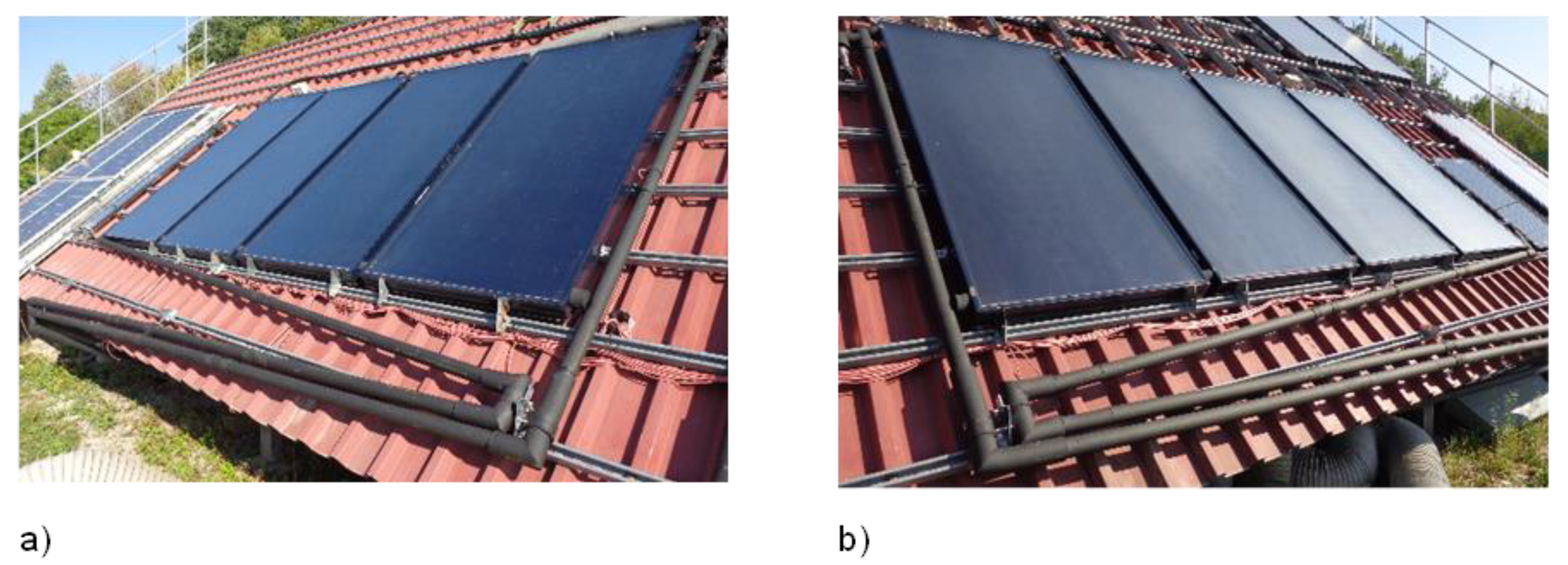
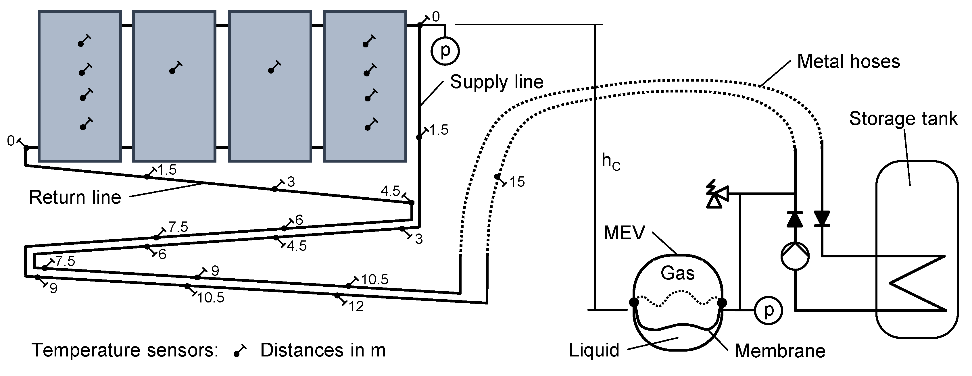
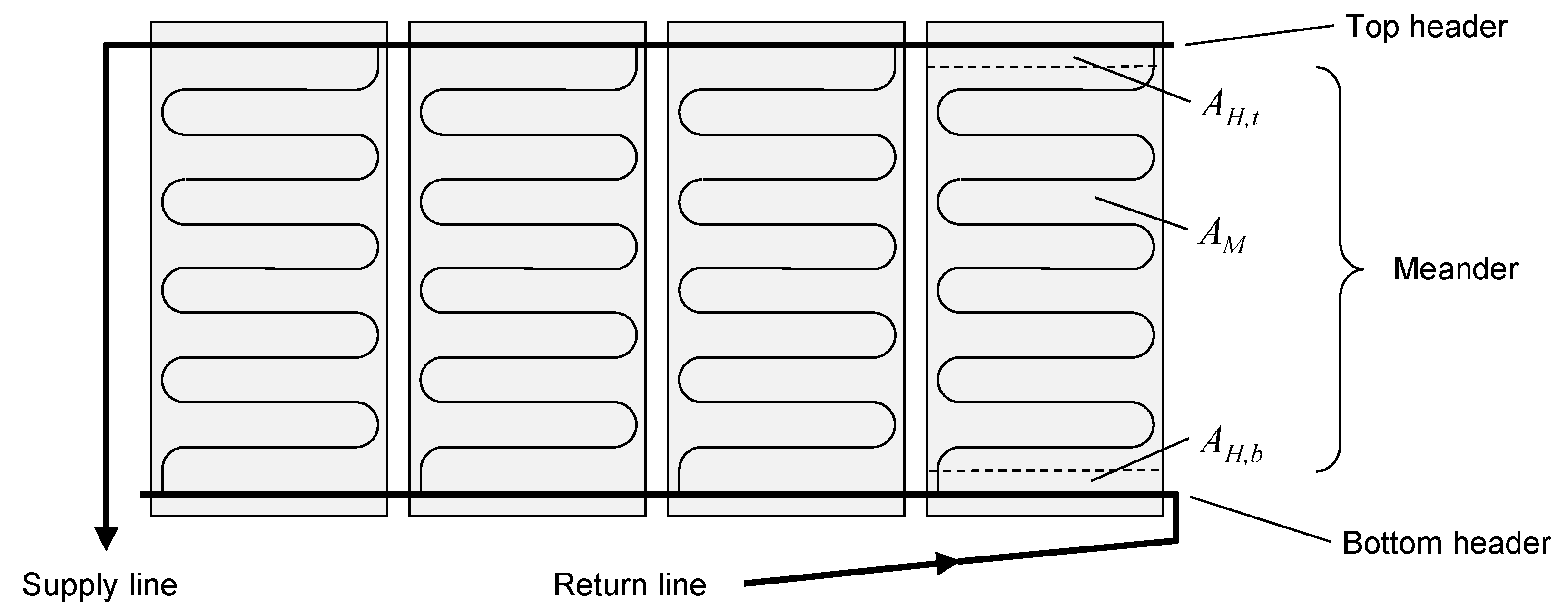
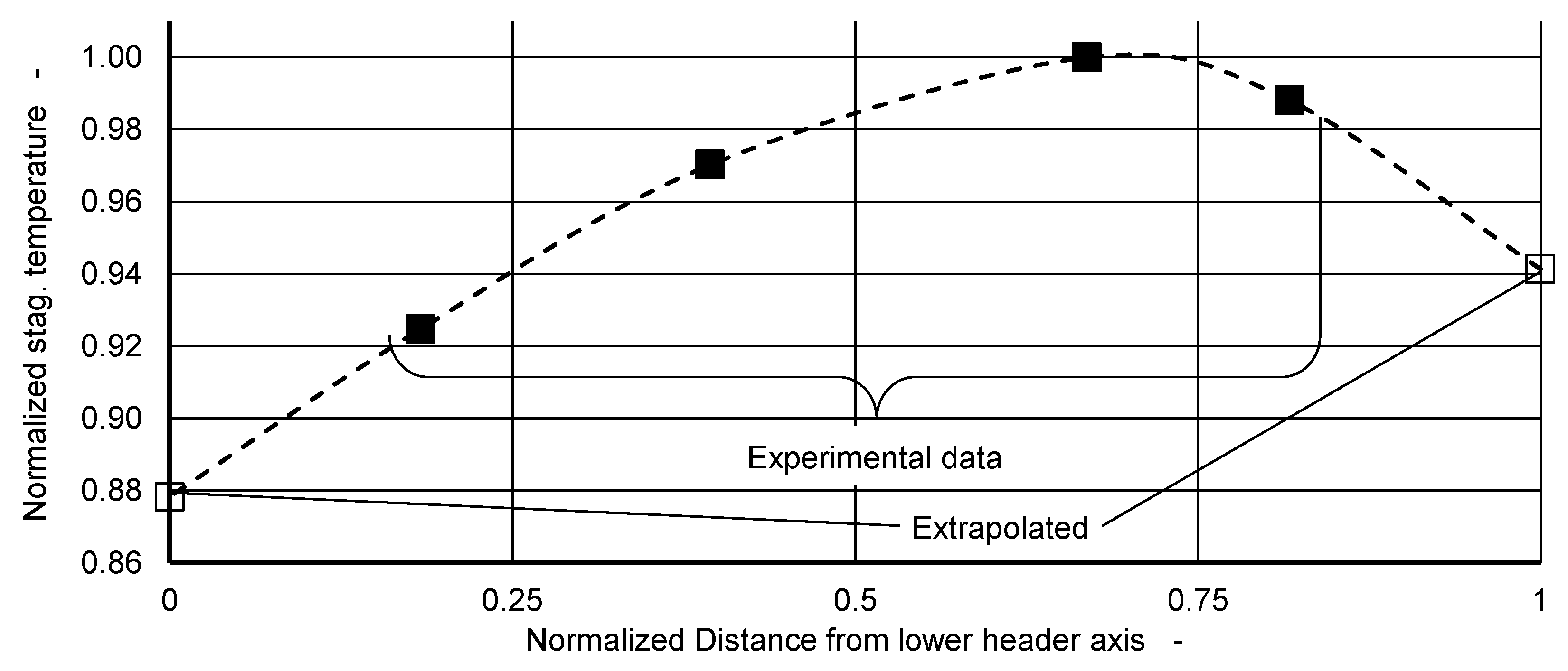
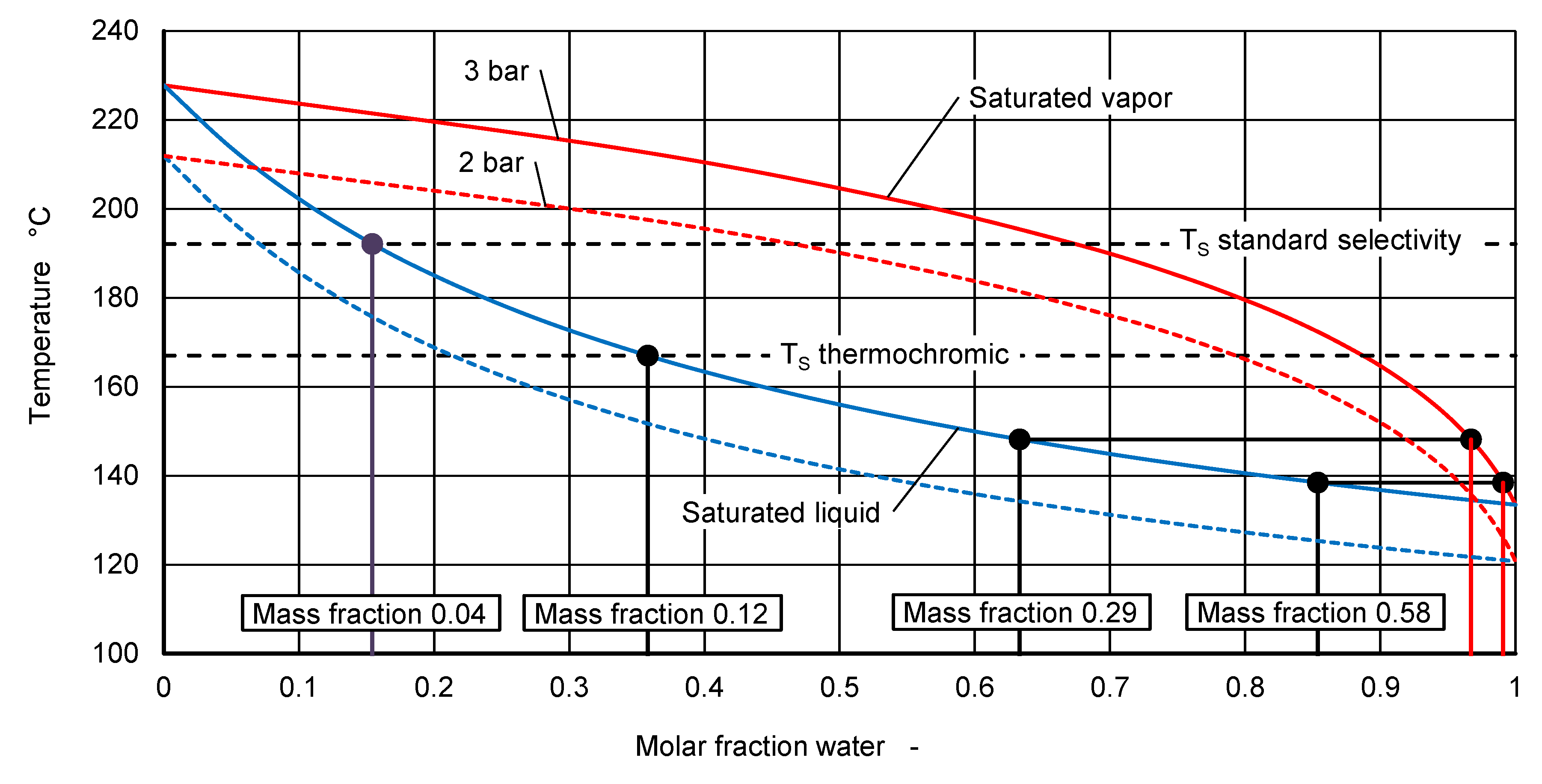
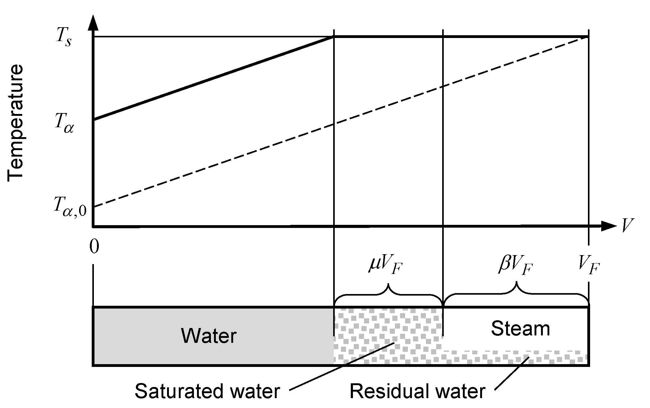
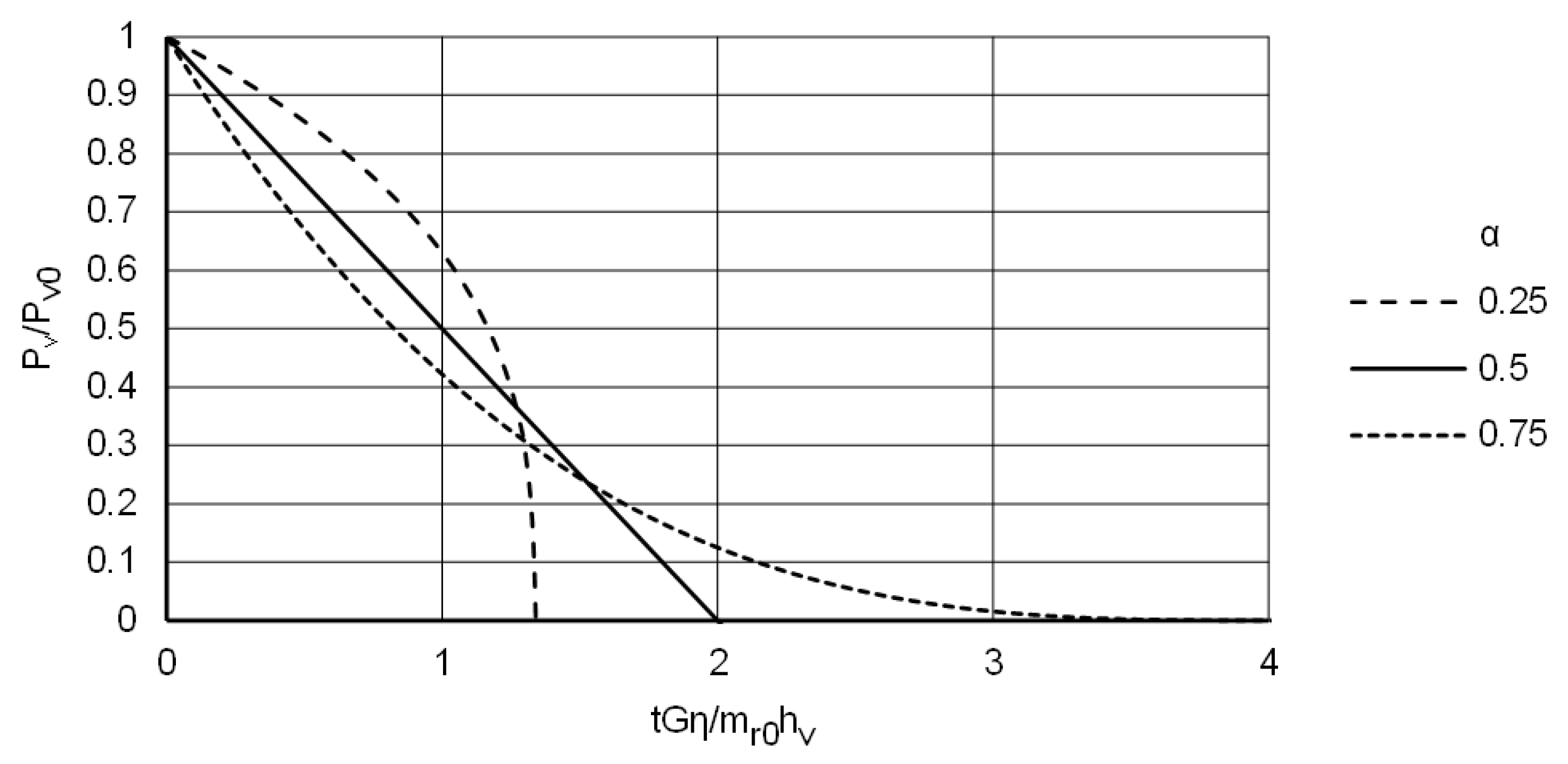
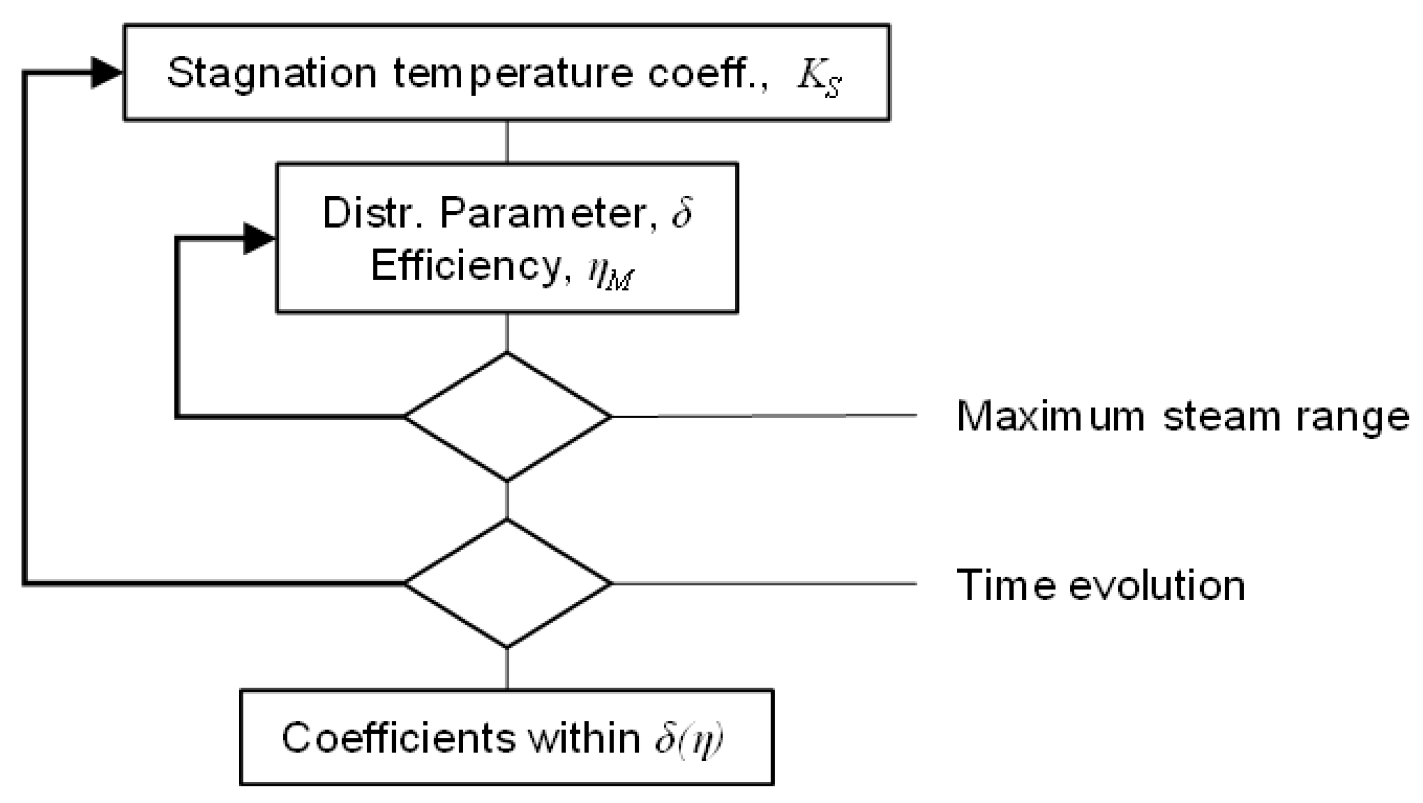
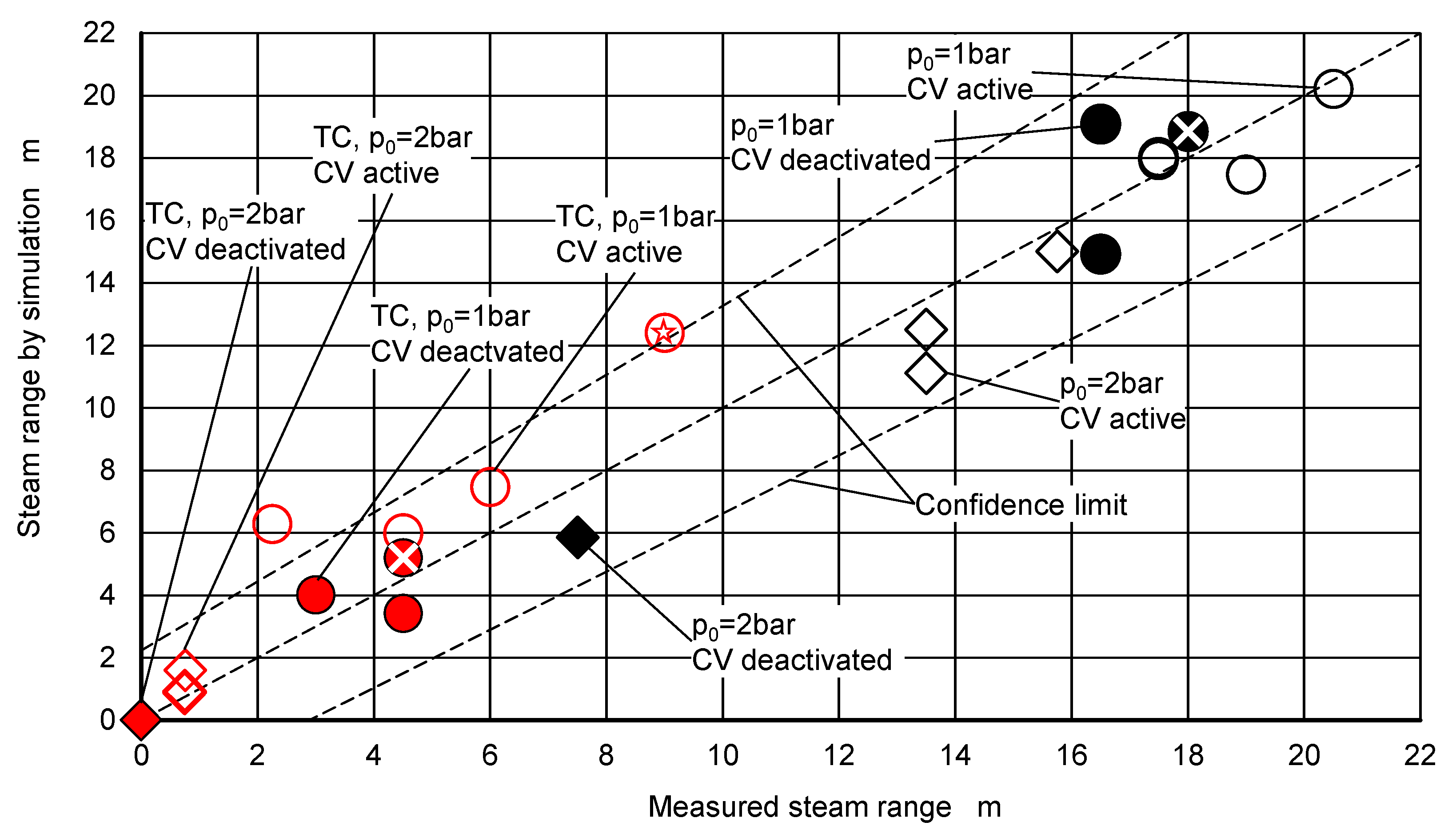
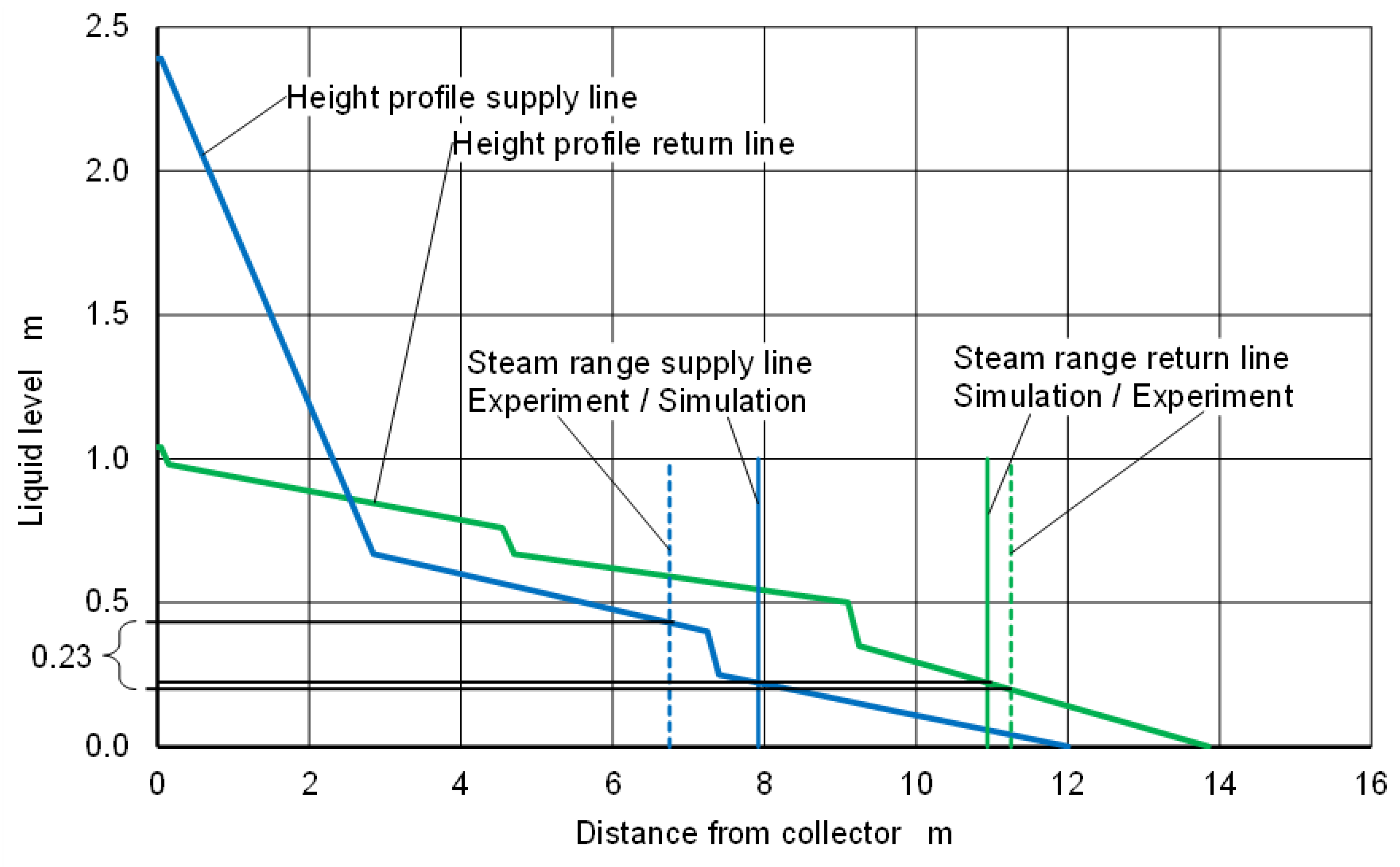
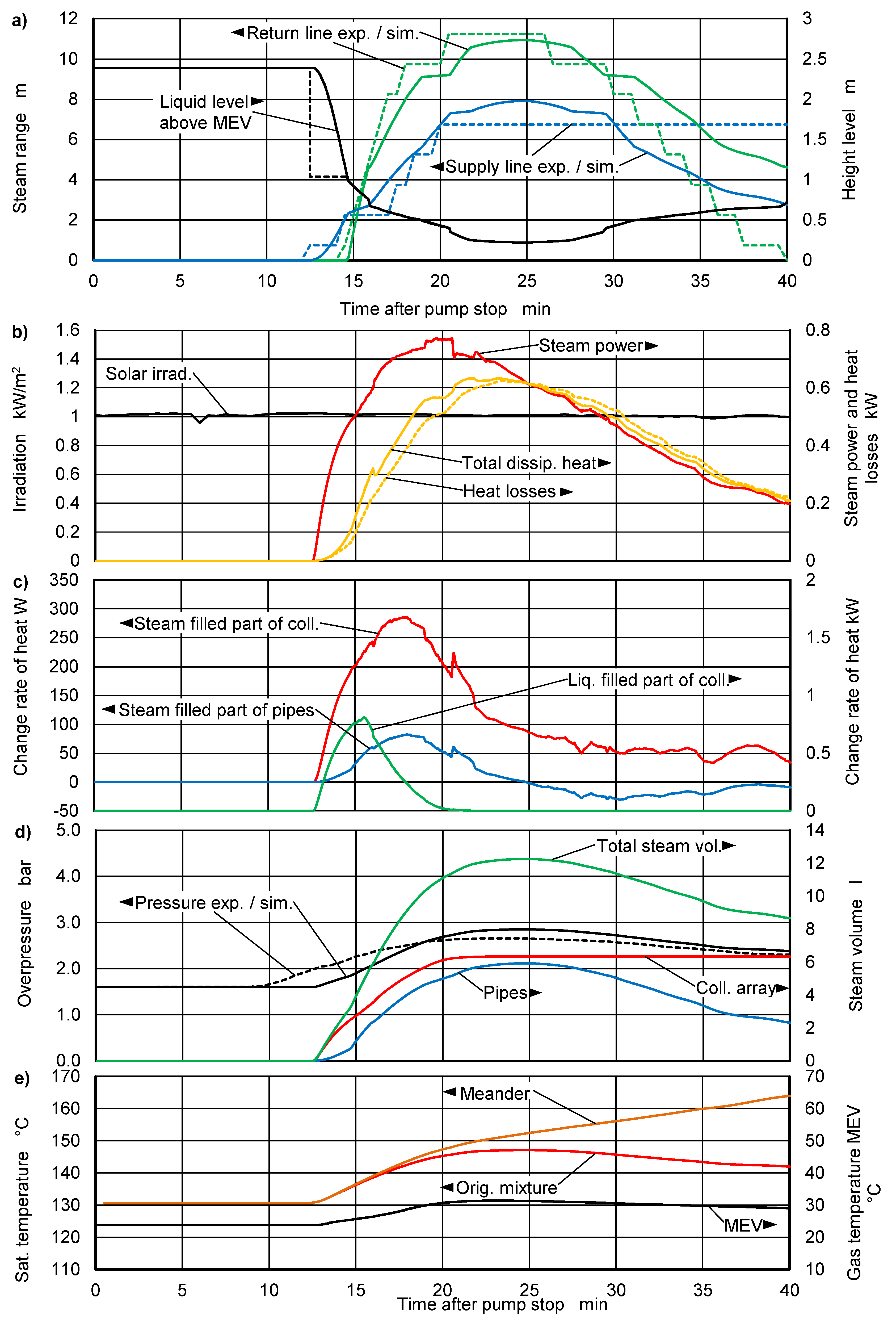
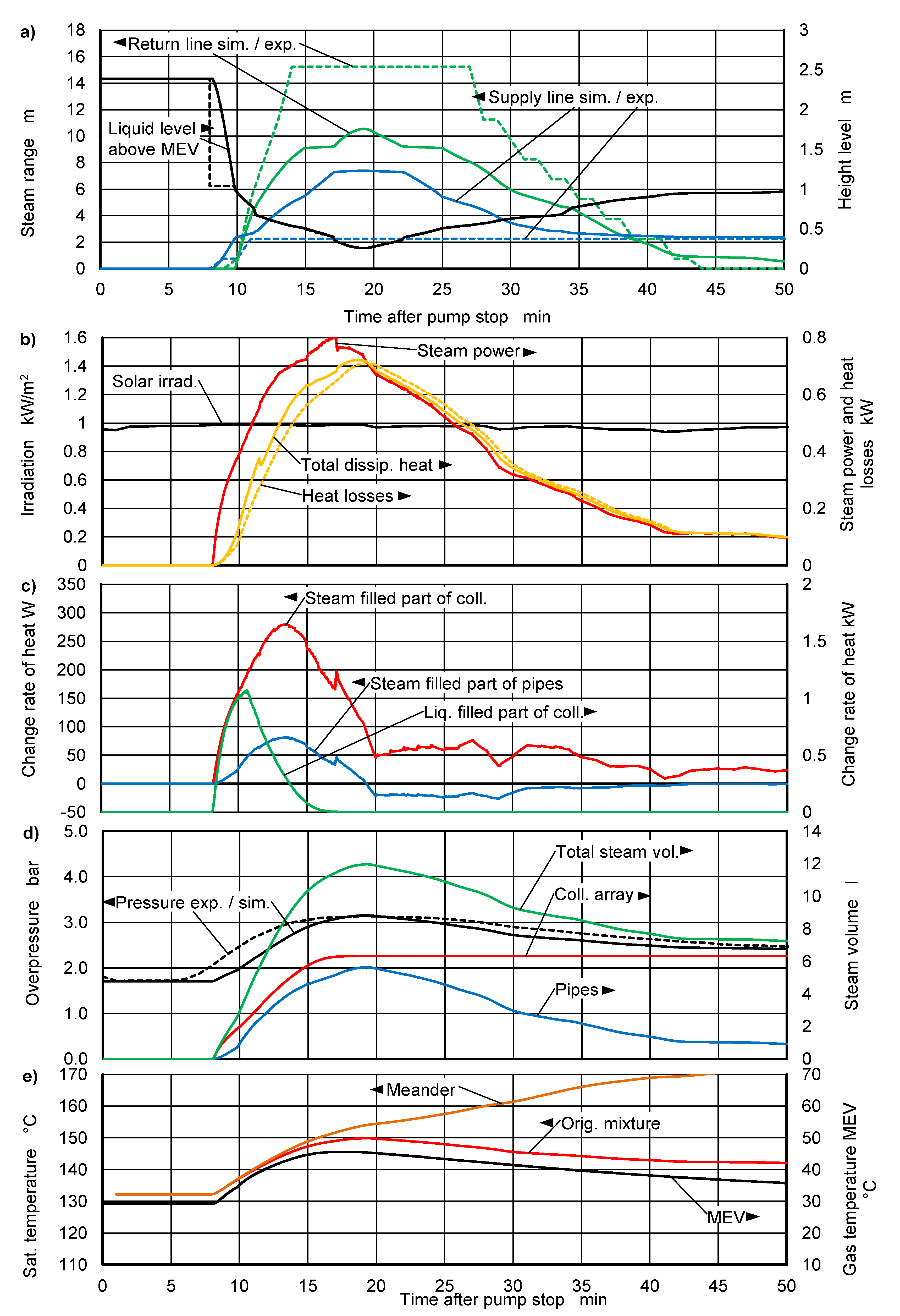
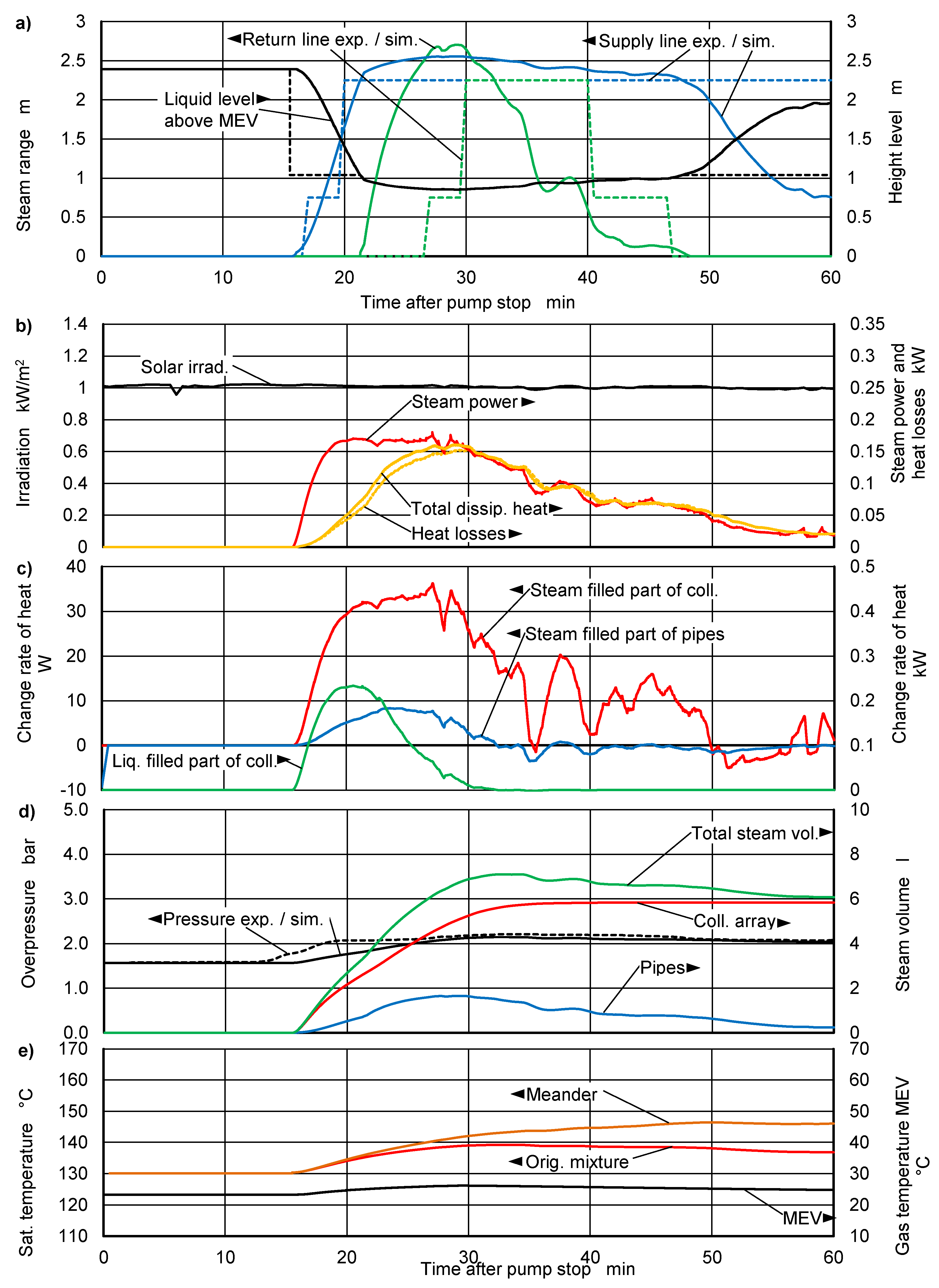
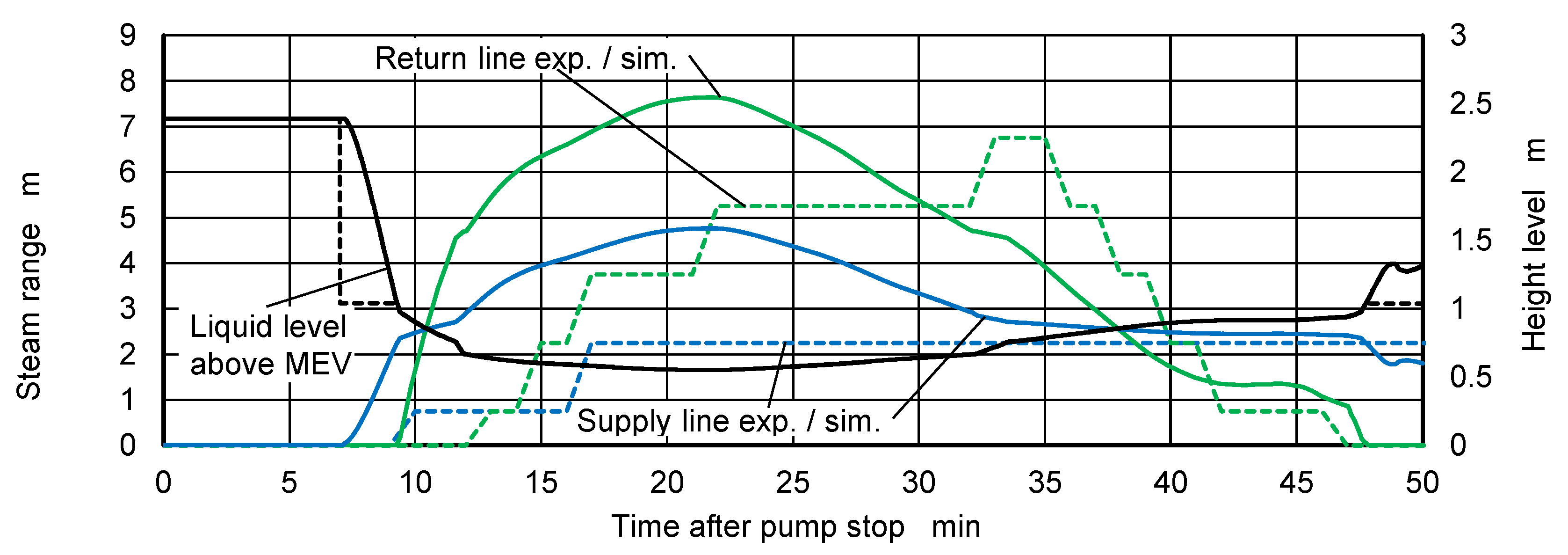
Table A1.
Model characteristics of collectors.
| Quantity | Unit | Standard | Thermochromic | |
|---|---|---|---|---|
| Critical temperature Tc | °C | - | 68 | |
| Temperature range | T ≤ Tc | T > Tc | ||
| zero-loss efficiency factor | - | η0 = 0.785 | η0 = 0.757 | η0,TC = 0.83 |
| Heat loss coefficient | W/Km2 | = 4.19 | = 4.27 | = 6.17 |
| Heat loss coefficient | W/K2m2 | = 0.0135 | = 0.0065 | = 0.0103 |
| Stagnation temperature | °C | 192.1 | 167 | |
| Dry meander region heat capacity | J/K | 2793 | ||
| Meander volume | l | 0.924 | ||
| Dry header region heat capacity | J/K | 566 | ||
| Header volume | l | 0.660 | ||
| Aperture area | m2 | 2.33 | ||
| Hydraulic elements | Length m | di m | Number of nodes - | |
| Absorber tube | 21.88 | 0.0082 | 88 | |
| Header tube | 1.1 | 0.02 | 1 | |
The material properties of the insulation layer are shown in Table A2. The optical properties have been estimated. The heat conductivity is modelled by a 2nd order polynomic based on the data-sheet [21],
Table A2.
Material properties of the pipe insulation.
| Heat Conductivity | W/Km | W/°C2m | W/°C3m |
|---|---|---|---|
| 0.03764 | 7.7 × 10−05 | 8 × 10−07 | |
| Absorption coefficient - | Emissivity - | Inner diameter mm | Outer diameter mm |
| 0.9 | 0.95 | 22 | 60 |
The properties of the pipe material used for the supply and return lines are listed in Table A3.
Table A3.
Properties of copper tubes.
| Inner Diameter | Outer Diameter | Density | Specific Heat | Conductivity |
|---|---|---|---|---|
| mm | mm | kg/m3 | J/kgK | W/Km |
| 20 | 22 | 8600 | 382 | 300 |
Properties of the Heat Carrier
A chemical analysis of the heat carrier TyfocorLS® yielded a mass fraction, , for the system with conventional selective absorbers and, xm0 = 0.557, for the system with thermochromic absorbers. The saturation temperature of the mixture is calculated based on the simplifying assumption of an ideal two-component mixture of water and propylene glycol using properties listed in Table A4. Within the temperature range considered here, the vapor pressure is sufficiently well described by a power function,
The coefficients listed in Table A4 are based on data from Steele, W. V. et al. [37] for propylene glycol, from D’Ans J., Lax E., Blachnik R. [38] for water and from the data sheet of TyfocorLS® [39].
Table A4.
Properties of water and propylene glycol.
| Molar Mass | Coefficients for Vapor Pressure in Pa | ||
|---|---|---|---|
| Component | kg/kmol | a | b |
| Water | 18.02 | 0.7517·10−3 | 4.047 |
| Propylene-glycol | 76.1 | 1.8745·10−8 | 5.601 |
| TyfocorLS | - | 0.7517·10−3 | 4.225 |
The specific heat capacity, density and viscosity are approximated by functions based on D’Ans et al. [38] for water and the data sheet of TyfocorLS® [39]. The surface tension of TyfocorLS® is modelled based on experimental data presented by Chang, et al. [40] for a binary mixture of propylene glycol with a molar fraction x = 0.85 of water.
Appendix B
Table A5.
Symbols and indices.
| Symbol | Unit | Symbol | Unit | ||
|---|---|---|---|---|---|
| A | m2 | Area | V | m3 | Volume |
| W/Km2 | Heat loss coefficient | W | Work rate | ||
| W/K2m2 | Heat loss coefficient | w | m/s | Velocity | |
| c | J/kgK | Specific heat capacity | wgj | m/s | Drift velocity |
| C | J/K | Heat capacity | x | m | Location of steam front |
| C0 | - | Distr. parameter | m/s | Velocity of steam front | |
| d | m | Diameter | x | - | Molar fraction |
| D | m | Outer diameter | xm | - | Mass fraction |
| G | W/m2 | Solar irradiation | Greek symbols | ||
| hC | m | Height difference | α | - | Steam power exponent |
| h | J/kg | Specific enthalpy | α | - | Absorption coefficient |
| hv | J/kg | Spec. evap. enthalpy | αc | W/Km2 | Conv. heat transfer coeff. |
| j | m/s | Superficial velocity | αr | W/Km2 | Rad. heat transfer coeff. |
| K | - | Correction factor | β | 1/K | Expansion coefficient |
| L | m | Char. length | β | - | Steam-filled fraction |
| l | m | Length | γ | - | View factor |
| m | kg | Mass | δ | - | Distribution parameter |
| kg/s | Mass flow | ε | - | Emissivity | |
| n | - | Number of nodes | η | - | Efficiency |
| nC | - | Number of collectors | λ | W/Km | Heat conductivity |
| ν | m2/s | Kinemat. viscosity | |||
| Pv | W | Steam power | Kg/m3 | Density | |
| p | Pa | Pressure | σ | Pa | Surface tension |
| W | Enthalpy change, gain | τ | s | Interval | |
| RD | - | Displacement ratio | φ | rad | Inclination angle |
| S | m2 | Surface | Dimensionless numbers | ||
| T | K, °C | Temperature | Nu | - | Nusselt number |
| UL | W/Km2 | Heat loss coefficient | Pr | - | Prandtl number |
| Ugj | m/s | Average drift velocity | Re | - | Reynolds number |
| u | J/kg | Specif. inner energy | Ra | - | Rayleigh number |
| Subscripts | |||||
| a | Ambient | i,k,q | Indices | ||
| C | Collector | ||||
| F | Field, array | S | Stagnation | ||
| G | Glycol | s | Saturation | ||
| g,l | Gas, liquid phase | t | Tube, pipe | ||
| H,b | Bottom header | v | Vapor | ||
| H,t | Top header | W | Water | ||
| i | Insulation | WG | Water-Glycol mixture | ||
| M | Meander | α | Inlet | ||
| m | Mean value | ω | Outlet | ||
| Constants | |||||
| g | Acceleration of gravity | 9.81 | m/s2 | ||
| σ | Stefan-Boltzmann constant | 5.67037·10−8 | W/K4m2 | ||
References
- Eismann, R. Thermohydraulik von Solaranlagen. Ph.D. Thesis, Eidgenössische Technische Hochschule ETH Zürich, Zürich, Switzerland, 2014. [Google Scholar]
- Terschueren, K.-H. Solaranlagen zur Brauchwassererwärmung, Anlagenkomponenten, Installation, Inbetriebnahme, Betriebsverhalten, Teil 2. IKZ-Haustechnik, Ausgabe 4. 1996. Available online: https://www.ikz.de/ikz-archiv/1996/04/9604118.php (accessed on 18 November 2020).
- Eismann, R.; von Felten, P. Stillstandsverhalten von Solaranlagen, Publikation 195200; 195200; Swiss Federal Ofice of Energy SFOE: Bern, Switzerland, 1998.
- Hausner, R.; Fink, C. Stagnation behaviour of solar thermal systems. In Proceedings of the ISES Europe Solar Congress, Copenhagen, Denmark, 19–22 June 2002. [Google Scholar]
- Hausner, R.; Fink, C. Stagnation Behaviour of Solar Thermal Systems—A Report of IEA SHC—Task 26—Solar Combisystems; International Energy Agency IEA: Paris, France, 2002.
- Streicher, W. Minimising the risk of water hammer and other problems at the beginning of stagnation of solar thermal plants—A theoretical approach. Solar Energy 2001, 69 (Suppl. 6), 187–196. [Google Scholar] [CrossRef]
- Lustig, K. Experimentelle Untersuchungen zum Stillstandsverhalten thermischer Solaranlagen. Ph.D. Thesis, University Karlsruhe, Karlsruhe, Germany, 2002. [Google Scholar]
- Hausner, R.; Fink, C.; Wagner, W.; Riva, R.; Hillerns, F. Entwicklung von Thermischen Solarsystemen mit Unproblematischem Stagnationsverhalten; Bundesministerium für Verkehr, Innovation und Technologie: Wien, Austria, 2003. [Google Scholar]
- Rommel, M.; Siems, T.; Schüle, K.; Mehnert, S.; Becker, R. Wieviel Dampf produziert ein Kollektor im Stillstandsfall? In Proceedings of 15th Symposium Thermische Solarenergie, Kloster Banz, Germany, 7–9 May 2014.
- Rommel, M.; Siems, T.; Schüle, K.; Mehnert, S.; Thoma, C. Schlussbericht zum Teilprojekt: Entwicklung von Techniken zur Beherrschung des Stillstandsbetriebes; Fraunhofer Gesellschaft für Solare Energiesysteme ISE: Freiburg, Germany, 2007. [Google Scholar]
- Scheuren, J.; Kirchner, M.; Eisenmann, W. Reduction of Stagnation Load of Large-Scale Collector Arrays. In Proceedings of the EuroSun, Glasgow, UK, 27–30 June 2006. [Google Scholar]
- Scheuren, J. Untersuchungen zum Stagnationsverhalten Solarthermischer Kollektorfelder. Ph.D. Thesis, Universität Kassel, Fachbereich Maschinenbau, Kassel University Press, Kassel, Germany, 2008. [Google Scholar]
- Harrison, S.; Cruickshank, C.A. A review of strategies for the control of high temperature stagnation in solar collectors and systems. Energy Procedia 2012, 30, 793–804. [Google Scholar] [CrossRef] [Green Version]
- Frank, E.; Mauthner, F.; Fischer, S. Overheating Prevention and Stagnation Handling in Solar Process Heat Applications—Technical Report A.1.2 of IEA SHC—Task 49—Solar Process Heat for Production and Advanced Applications; International Energy Agency IEA: Paris, France, 2015.
- Freixa, J.; Kim, T.-W.; Manera, A. Thermal-hydraulic analysis of an intermediate LOCA test at the ROSA facility including uncertainty evaluation. Nucl. Eng. Design 2012, 249, 97–103. [Google Scholar] [CrossRef]
- U.S.NRC. TRACE V5. 0 Theory Manual. Field Equations, Solution Methods, and Physical Models; Division of Risk Assessment and Special Projects, Office of Nuclear Regulatory Research, US Nuclear Regulatory Commission: Washington, DC, USA, 2007.
- Eismann, R.; Föller, F.; Witzig, A. Programm THD: Thermohydraulisches Dimensionierungsprogramm für Solaranlagen. Schlussbericht; Bundesamt für Energie BFE: Bern, Switzerland, 2017. [Google Scholar]
- Müller, S.; Reineke-Koch, R.; Giovannetti, F.; Hafner, B. Experimental Investigations on the Stagnation Behavior of Thermochromic Flat Plate Collectors. In Proceedings of the EuroSun, Rapperswil, Switzerland, 10–13 September 2018. [Google Scholar]
- CEN. EN-12975-2, Thermische Solaranlagen und ihre Bauteile—Kollektoren. In Teil 2: Prüfverfahren; Beuth Verlag GmbH: Berlin, Germany, 2006. [Google Scholar]
- Eismann, R. Accurate analytical modeling of flat plate solar collectors: Extended correlation for convective heat loss across the air gap between absorber and cover plate. Solar Energy 2015, 122, 1214–1224. [Google Scholar] [CrossRef] [Green Version]
- Armacell. HT/ArmaFlex—The Flexible Insulation for High Temperature Applications. Available online: https://local.armacell.com/fileadmin/cms/uk/products/en/HTArmaFlexRangeUKROI.pdf (accessed on 18 November 2020).
- Adelard, L.; Pignolet-Tardan, F.; Mara, T.; Lauret, P.; Garde, F.; Boyer, H. Sky temperature modelisation and applications in building simulation. Renew. Energy 1998, 15, 418–430. [Google Scholar] [CrossRef]
- Churchill, S.W. A comprehensive correlating equation for laminar, assisting, forced and free convection. AIChE J. 1977, 23, 10–16. [Google Scholar] [CrossRef]
- Churchill, S.W.; Chu, H.H. Correlating equations for laminar and turbulent free convection from a horizontal cylinder. Int. J. Heat Mass Transf. 1975, 18, 1049–1053. [Google Scholar] [CrossRef]
- Gnielinski, V. Berechnung mittlerer Wärme- und Stoffübergangskoeffizienten an laminar und turbulent überströmten Einzelkörpern mit Hilfe einer einheitlichen Gleichung. Forsch Ing. 1975, 41, 145–153. [Google Scholar] [CrossRef]
- Tetsu, F.; Haruo, U. Laminar natural-convective heat transfer from the outer surface of a vertical cylinder. Int. J. Heat Mass Transf. 1970, 13, 607–615. [Google Scholar] [CrossRef]
- Raithby, G.D.; Hollands, K.G.T. A General Method of Obtaining Approximate Solutions to Laminar and Turbulent Free Convection Problems. Adv. Heat Transf. 1975, 11, 265–315. [Google Scholar] [CrossRef]
- Dropkin, D.; Somerscales, E. Heat transfer by natural convection in liquids confined by two parallel plates which are inclined at various angles with respect to the horizontal. J. Heat Transfer. 1965, 87, 77–82. [Google Scholar] [CrossRef]
- Zuber, N.; Findlay, N.A. Average Volumetric Concentration in Two-Phase Systems. Trans. ASME Ser. C J. Heat Transf. 1965, 87, 453–468. [Google Scholar] [CrossRef]
- Coddington, P.; Macian, R. A study of the performance of void fraction correlations used in the context of drift-flux two-phase flow models. Nucl. Eng. Design 2002, 215, 199–216. [Google Scholar] [CrossRef]
- Choi, J.; Pereyra, E.; Sarica, C.; Park, C.; Kang, J. An Efficient Drift-Flux Closure Relationship to Estimate Liquid Holdups of Gas-Liquid Two-Phase Flow in Pipes. Energies 2012, 5, 5294–5306. [Google Scholar] [CrossRef] [Green Version]
- Kirkup, L.; Frenkel, R. An Introduction to Uncertainty in Measurement: Using the GUM (Guide to the Expression of Uncertainty in Measurement); Cambridge University Press: Cambridge, UK, 2006. [Google Scholar]
- Kovacs, P. A Guide to the Standard EN 12975; SP—Technical Research Institute of Sweden: Borås, Sweden; European Solar Thermal Industry Federation (ESTIF): Brussels, Belgium, 2012. [Google Scholar]
- Chexal, B.; Lellouche, G.; Horowitz, J.; Healzer, J. A void fraction correlation for generalized applications. Prog. Nucl. Energy 1992, 27, 255–295. [Google Scholar] [CrossRef]
- Bhagwat, S.M.; Ghajar, A.J. A flow pattern independent drift flux model based void fraction correlation for a wide range of gas–liquid two phase flow. Int. J. Multiph. Flow 2014, 59, 186–205. [Google Scholar] [CrossRef]
- Eismann, R. Cost reduction of solar thermal plants by advanced thermalhydraulic design methods. In Proceedings of the CISBAT 2019, Lausanne, Switzerland, 4–6 September 2019. [Google Scholar]
- Steele, W.V.; Chirico, R.D.; Knipmeyer, S.E.; Nguyen, A. Measurements of Vapor Pressure, Heat Capacity, and Density along the Saturation Line for ε-Caprolactam, Pyrazine, 1,2-Propanediol, Triethylene Glycol, Phenyl Acetylene, and Diphenyl Acetylene. J. Chem. Eng. Data 2002, 47, 689–699. [Google Scholar] [CrossRef]
- D’Ans, J.; Lax, E.; Blachnik, R. Taschenbuch für Chemiker und Physiker: Band 3: Elemente, anorganische Verbindungen und Materialien, Minerale: Bd. III; Springer: Berlin/Heidelberg, Germany, 1998. [Google Scholar]
- TYFOROP. Technical Information: TYFOCOR LS. Available online: https://www.tyfo.de/uploads/TI/Ti_TYFOCOR-LS_gb.pdf (accessed on 8 July 2020).
- Chang, C.-W.; Hsiung, T.-L.; Lui, C.-P.; Tu, C.-H. Densities, surface tensions, and isobaric vapor–liquid equilibria for the mixtures of 2-propanol, water, and 1,2-propanediol. Fluid Phase Equilibria 2015, 389, 28–40. [Google Scholar] [CrossRef]
Figure 1.
Array of four flat-plate collectors with (a) thermochromic absorbers and (b) standard selective absorbers.
Figure 1.
Array of four flat-plate collectors with (a) thermochromic absorbers and (b) standard selective absorbers.

Figure 2.
Hydraulic diagram of the circuit, components and temperature sensor positions, valid for both systems.
Figure 2.
Hydraulic diagram of the circuit, components and temperature sensor positions, valid for both systems.

Figure 3.
Solar collector array with meander-shaped absorber tubes and integrated header tubes connected in parallel.
Figure 3.
Solar collector array with meander-shaped absorber tubes and integrated header tubes connected in parallel.

Figure 4.
Collector efficiency curves for conventional selective coating (black lines) and thermochromic coating (red lines), valid for G = 1000 W/m2 and Ta = 30 °C.
Figure 4.
Collector efficiency curves for conventional selective coating (black lines) and thermochromic coating (red lines), valid for G = 1000 W/m2 and Ta = 30 °C.

Figure 5.
Normalized temperature distribution during dry stagnation, as a function of the distance from the lower header axis. The black markers indicate values measured.
Figure 5.
Normalized temperature distribution during dry stagnation, as a function of the distance from the lower header axis. The black markers indicate values measured.

Figure 6.
Phase diagram of water propylene glycol at three bar absolute pressure.

Figure 7.
Thermodynamic states within a stagnating collector field during displacement.

Figure 8.
Relative enthalpy flow of steam as a function of dimensionless time.

Figure 9.
Procedure to determine model parameters.

Figure 10.
Comparison of total steam ranges from experimental data and simulations for the system with thermochromic absorbers (red) and conventional selective absorbers (black). Markers with white crosses correspond to the dataset 08−16. The marker with a red star corresponds to the dataset 07−25.
Figure 10.
Comparison of total steam ranges from experimental data and simulations for the system with thermochromic absorbers (red) and conventional selective absorbers (black). Markers with white crosses correspond to the dataset 08−16. The marker with a red star corresponds to the dataset 07−25.

Figure 11.
Height profiles of the supply and return lines.

Figure 12.
Experimental and simulation results for the system with standard selective absorbers. Opened check valves. Case 08−16. (a) Steam range and level height, (b) Steam power, heat losses and irradiation, (c) Change rates of heat, (d) Overpressure and steam volume, (e) Saturation temperature and gas temperature inside MEV.

Figure 13.
Experimental and simulation results for the system with standard selective absorbers. Active check valves. Dataset 07−26. (a) Steam range and level height, (b) Steam power, heat losses and irradiation, (c) Change rates of heat, (d) Overpressure and steam volume, (e) Saturation temperature and gas temperature inside MEV.

Figure 14.
Experimental and simulation results for the system with thermochromic absorbers. Inactive check valves. Dataset 08−16. (a) Steam range and level height, (b) Steam power, heat losses and irradiation, (c) Change rates of heat, (d) Overpressure and steam volume, (e) Saturation temperature and gas temperature inside MEV.

Figure 15.
Steam range from experiment and simulation for the system with thermochromic absorbers. Active check valves. Dataset 07−25.
Figure 15.
Steam range from experiment and simulation for the system with thermochromic absorbers. Active check valves. Dataset 07−25.

Table 1.
Propagation parameters and pipe direction with respect to the inlet and outlet of the collector field.
Table 1.
Propagation parameters and pipe direction with respect to the inlet and outlet of the collector field.
| Supply Line | Return Line | ||
|---|---|---|---|
| horizontal | horizontal | 1 | 1 |
| horizontal | downward | 1 | 0 |
| downward | horizontal | 0 | 1 |
| downward | downward | 1 | 1 |
Table 2.
Average irradiation on the system with the standard selective (SC) and thermochromic (TC) absorber coating. Experimental and simulation results of the total steam range and simulation results of the residual mass. Active check valves (CV) are indicated by “✓”.
Table 2.
Average irradiation on the system with the standard selective (SC) and thermochromic (TC) absorber coating. Experimental and simulation results of the total steam range and simulation results of the residual mass. Active check valves (CV) are indicated by “✓”.
| Dataset | CV | p0 | <G> | Residual Mass | Total Steam Range | |||||
|---|---|---|---|---|---|---|---|---|---|---|
| mm−dd | - | Bar | W/m2 | W/m2 | kg | kg | m | m | ||
| SC | TC | SC | TC | SC | TC | SC | TC | |||
| Exp. | Exp. | Sim. | Sim. | Exp. | Exp. | Sim. | Sim. | |||
| 07−24 | ✓ | 1 | 960 | 960 | 1.61 | 2.24 | 19.0 | 4.5 | 17.5 | 6.0 |
| 07−25 | ✓ | 1 | 1014 | 1014 | 1.52 | 1.74 | 20.5 | 9.0 | 20.2 | 12.4 |
| 07−26 | ✓ | 1 | 960 | 956 | 1.60 | 2.16 | 17.5 | 2.3 | 18.0 | 6.3 |
| 07−27 | ✓ | 1 | 902 | 903 | 1.63 | 2.17 | 20.5 | 6.5 | 19.6 | 7.5 |
| 08−02 | ✓ | 2 | 960 | 960 | 2.03 | 6.59 | 13.5 | 0.8 | 11.1 | 0.9 |
| 08−03 | ✓ | 2 | 988 | 988 | 1.78 | 3.72 | 15.8 | 0.8 | 15.0 | 1.6 |
| 08−06 | ✓ | 2 | 997 | 997 | 1.89 | 5.15 | 13.5 | 0.8 | 12.5 | 0.9 |
| 08−16 | − | 1 | 986 | 990 | 1.59 | 2.40 | 18.0 | 4.5 | 18.9 | 5.2 |
| 09−04 | − | 1 | 892 | 890 | 1.82 | 6.90 | 16.5 | 4.5 | 14.9 | 3.4 |
| 09−05 | − | 1 | 948 | 950 | 1.61 | 2.70 | 16.5 | 3.0 | 19.1 | 4.0 |
| 09−18 | − | 2 | 948 | 948 | 2.39 | 6.83 | 7.5 | 0.0 | 5.9 | 0.0 |
Table 3.
Uncertainties of material properties and boundary conditions and their effect on the simulated steam range, based on data set 08−16.
Table 3.
Uncertainties of material properties and boundary conditions and their effect on the simulated steam range, based on data set 08−16.
| Quantity | Uncertainty | Effect on Steam Range M | |
|---|---|---|---|
| Standard | Thermochromic | ||
| Solar irradiance | ±2% | +1.06/−1.01 | +0.87/−0.90 |
| Collector efficiency | ±4% | +0.49/−0.49 | +0.17/−0.28 |
| Preset gauge pressure 1bar | ±0.1 bar | +0.46/−0.51 | +0.22/−0.34 |
| Heat conductivity of pipe insulation | ±10% | −0.8/+0.96 | −0.3/+0.32 |
Table 4.
Relative uncertainty to be used in system dimensioning.
| Absorber Type | Steam Range | Average Uncertainty | Relative Uncertainty |
|---|---|---|---|
| m | m | - | |
| Conventional selective | 18 | 4.0 | 0.22 |
| Thermochromic | 4.5 | 2.9 | 0.63 |
Publisher’s Note: MDPI stays neutral with regard to jurisdictional claims in published maps and institutional affiliations. |
© 2021 by the authors. Licensee MDPI, Basel, Switzerland. This article is an open access article distributed under the terms and conditions of the Creative Commons Attribution (CC BY) license (http://creativecommons.org/licenses/by/4.0/).
Share and Cite
MDPI and ACS Style
Eismann, R.; Hummel, S.; Giovannetti, F. A Thermal-Hydraulic Model for the Stagnation of Solar Thermal Systems with Flat-Plate Collector Arrays. Energies 2021, 14, 733. https://doi.org/10.3390/en14030733
AMA Style
Eismann R, Hummel S, Giovannetti F. A Thermal-Hydraulic Model for the Stagnation of Solar Thermal Systems with Flat-Plate Collector Arrays. Energies. 2021; 14(3):733. https://doi.org/10.3390/en14030733
Chicago/Turabian StyleEismann, Ralph, Sebastian Hummel, and Federico Giovannetti. 2021. "A Thermal-Hydraulic Model for the Stagnation of Solar Thermal Systems with Flat-Plate Collector Arrays" Energies 14, no. 3: 733. https://doi.org/10.3390/en14030733
Note that from the first issue of 2016, this journal uses article numbers instead of page numbers. See further details here.