Role of Inflow Turbulence and Surrounding Buildings on Large Eddy Simulations of Urban Wind Energy
by
 , , ,
, , ,
Giulio Vita
1,2,* ,
,
Syeda Anam Hashmi
2 ,
,
Simone Salvadori
3 ,
,
Hassan Hemida
2 and 
Charalampos Baniotopoulos
2 1
Dipartimento di Ingegneria Industriale—DIEF, Università degli Studi Firenze, 50139 Firenze, Italy
2
Department of Civil Engineering, School of Engineering, University of Birmingham, Edgbaston, Birmingham B15 2TT, UK
3
Dipartimento Energia—DENERG, Politecnico di Torino, 10129 Torino, Italy
*
Author to whom correspondence should be addressed.
Energies 2020, 13(19), 5208; https://doi.org/10.3390/en13195208
Submission received: 4 September 2020
/
Revised: 29 September 2020
/
Accepted: 2 October 2020
/
Published: 6 October 2020
(This article belongs to the Special Issue Advances in Wind Energy Structures)
Abstract
:Predicting flow patterns that develop on the roof of high-rise buildings is critical for the development of urban wind energy. In particular, the performance and reliability of devices largely depends on the positioning strategy, a major unresolved challenge. This work aims at investigating the effect of variations in the turbulent inflow and the geometric model on the flow patterns that develop on the roof of tall buildings in the realistic configuration of the University of Birmingham’s campus in the United Kingdom (UK). Results confirm that the accuracy of Large Eddy Simulation (LES) predictions is only marginally affected by differences in the inflow mean wind speed and turbulence intensity, provided that turbulence is not absent. The effect of the presence of surrounding buildings is also investigated and found to be marginal to the results if the inflow is turbulent. The integral length scale is the parameter most affected by the turbulence characteristics of the inflow, while gustiness is only marginally influenced. This work will contribute to LES applications on the urban wind resource and their computational setup simplification.
1. Introduction
Urban wind energy (UWE) is a branch of wind energy which has shown poor success, questioning not only the sensibility of harvesting wind in the urban environment, but also hampering the public image of the whole wind energy sector [1]. Key to a good positioning strategy is through predicting flows in the urban environment [2,3]. However, simulations specifically tailored to assess the wind energy resource have only been conducted in a handful of studies, all reviewed in a recent significant paper [4]. Of the studies focusing on the wind energy resource, only 18% deals with a realistic urban setup, and 10% is conducted using Large Eddy Simulations (LES) [4], a numerical technique able to solve the inertial scales of turbulent flows. Most research implements Reynolds averaged Navier-Stokes (RANS) models to predict wind conditions found in urban areas [4]. In fact, only a single study has specifically modelled urban winds for wind energy harvesting purposes using LES over a non-uniform array of cubes [5]. The majority of studies on urban wind energy focus on the parametrization of the shape of high-rise buildings aimed at maximizing mean wind speed and minimizing turbulence, often without addressing the validation of results or attempting to deepen the knowledge on how turbulence is generated from the building or how turbulent coherent structures interact with obstacles [2,6,7].
LES has been used successfully in research about the urban wind flow, as it allows one to overcome the limitations of wind tunnel testing and provides an accurate description of the fluctuating flow field [3]. However, LES studies on urban wind are mainly focused on replicating wind tunnel data [4,8], i.e., not exploiting the technique for its potential of expanding wind tunnel results. The lack of best practice guidelines (BPGs) is recognized as a major drawback to the use of LES in practical engineering problems, as well as the relative paucity of results showing the performance of LES in predicting an accurate and reliable flow field in a urban environment. The lack of a validation strategy tailored to the problem at stake is the main obstacle for LES to be practically feasible in urban flow research [9]. Or rather, the validation of a numerical model for a specific statistic in a specific location is not a guarantee of the accuracy of the overall simulation [10]. In fact, the validation of Computational Fluid Dynamics (CFD) applications made with reference to the boundary layer development above specific locations or alignments within the urban area of interest, e.g., above the building heights or at the inlet, might very possibly not be evidence of the quality of urban winds assessment [11]. This is especially worrisome if the most convenient use of CFD is made: extending the experimental scope beyond its physical limitations (e.g., varying wind or geometry characteristics) [12].
Wind tunnel modelling remains the main approach to address urban flows and the foremost source of validation database. Most knowledge on wind tunnel testing accuracy for urban flows is founded on pressure measurements, and very few measurements are available on the actual flow field. Furthermore, due to the scaling of the geometry, wind tunnel measurements have strong limitations. In particular close to walls and surfaces, it is difficult to obtain but a coarse number of measurement positions, while the uneven directionality of the flow field, the low wind velocities, and the reduced distance between probes and model’s surfaces might affect the sensor performance, impacting the assessment of the flow [13,14,15,16]. Furthermore, the omission of thermal and stratification effects might also represent a challenging limitation inside the urban plume, where thermal effects are known to modify the atmosphere physics significantly [17]. That is the reason why the validation of RANS or LES studies remains challenging, and it must be appropriately setup, i.e., it has to be done in those areas of interest for which the CFD simulation is specifically tailored [18,19].
This study spurs from research done at the University of Birmingham on pedestrian level winds [20]. The adequacy of various physical and numerical simulation techniques has been tested to assess pedestrian distress in full-scale conditions. While the performance of LES evidently outperforms RANS at pedestrian level and above the roof [21] and closely competes with hot-wire anemometry measurements, an interesting result has been noted. The inflow turbulence as measured in the wind tunnel is not accurately predicted in the LES, due to differences in the computational domain to reduce computational costs. Nevertheless, the remarkable accuracy of results suggests that close to high-rise buildings the flow is only influenced by the building and its features, meaning that turbulence at the inflow only has a marginal effect on the assessment of the flow field where of interest. Recent works seems to agree that the flow field across the domain might be divided into a far-from-buildings region showing a strong sensitivity to the inlet profile, and a through-buildings region where the behavior seems rather insensitive [22]. As an increasing number of LES studies on simplified geometries investigate the possibility of introducing a suitable turbulent inlet to correct for the spatial limitedness of the computational domain [23], it is not clear how an inlet profile matching mean wind speed and turbulence intensity might guarantee on the description of the fluctuating flow behavior over a complex urban setup [24,25].
This work aims at understanding the variability of the flow pattern above high-rise buildings in a realistic urban configuration under varying turbulent inflow conditions. The work adds to the rather limited results on LES applicability to urban wind assessment and provides some indications to practitioners which might contribute to the building of much needed LES BPGs for the urban environment. As the work is validated extensively in previous research using wind tunnel testing [20,21], this pure numerical study explores a variety of geometries and domain to understand the feasibility of LES as a cost-effective tool for the prediction of the urban wind above high-rise buildings, which is of interest for urban wind energy and structural safety applications. The Campus of the University of Birmingham (UoB) in the UK is simulated with various configurations and results focus on its two high-rise buildings. The model is ancillary to a broader research on pedestrian distress in urban winds, reported in detail in [20].
2. Methodology
2.1. Framework of the Research
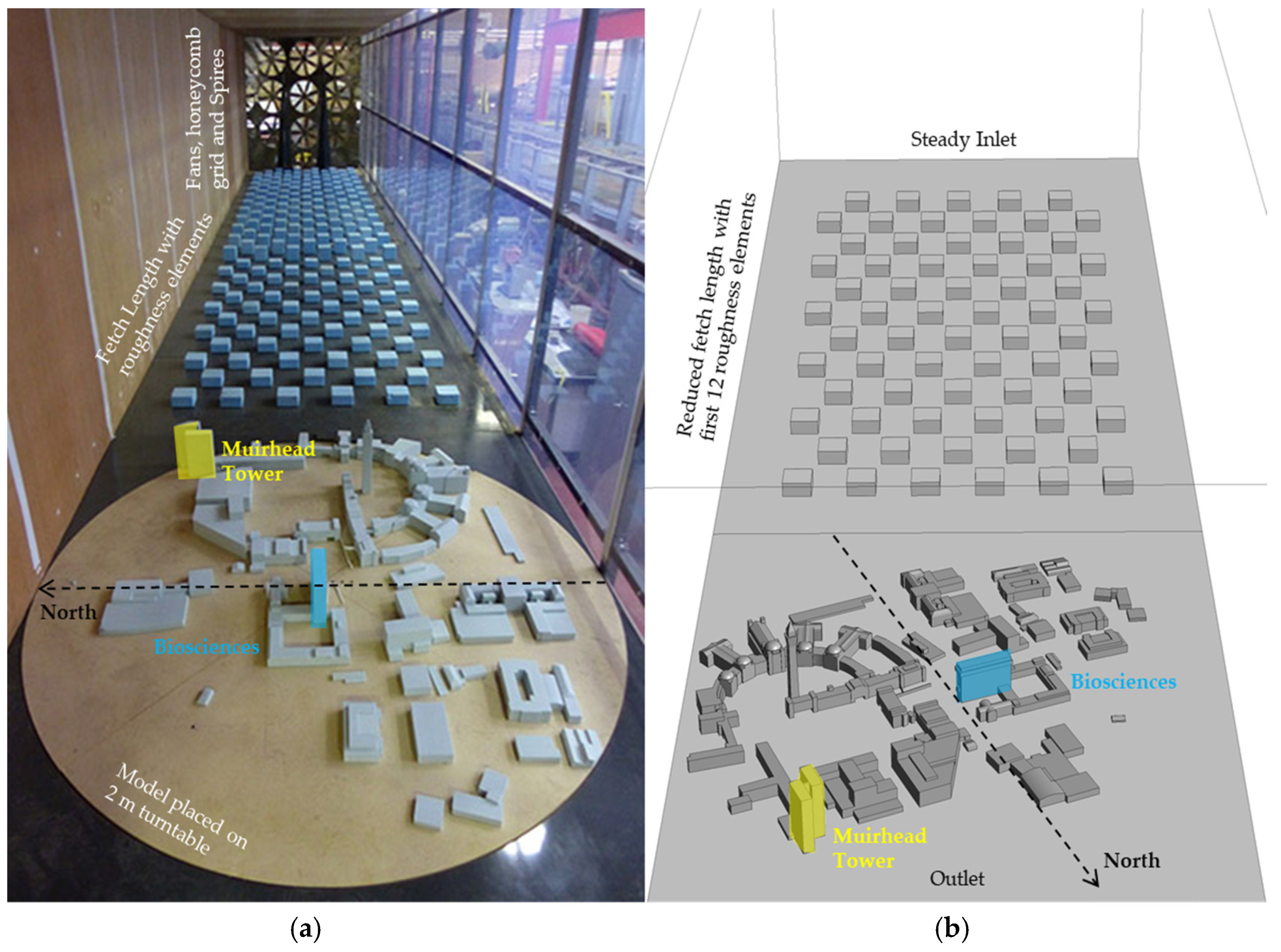
The “Urban Winds” research project comprises a full-scale field test conducted during an experimental campaign at the UoB campus, with the campus being a good representation of high-rise buildings insisting on a typical urban environment. The setup is then reproduced using physical and numerical simulations, compared in a detailed way to understand the adequacy of low- and high-fidelity methods for predicting the behavior [20]. Measurements were taken during a major disruptive wind event, namely storm Ophelia occurring on the 12 October 2017 in the United Kingdom. The storm blew from South-South-West (SSW, 203° from North), and this configuration was replicated in physical and numerical simulations.
The two high-rise buildings chosen are the Muirhead tower and the Biosciences tower. The 62 m tall Muirhead Tower (MT) is placed in the northeastern part of the campus, and in the wind tunnel test it lies at the limit of the 2 m wide test platform (Figure 1). The 42 m tall Biosciences tower (BB) is placed instead at the center of the platform, where pedestrian level measurements are taken at a height of 2 m above the ground as within the scope of the research framework this study is part of.
In wind tunnel tests, it was possible to obtain measurements in other positions than the pedestrian test-route of the study, i.e., above the roof of both towers. Unfortunately, the relevant full-scale measurements are not available at those positions, as only a reference sonic anemometer is placed 10 m on top of the Muirhead tower.
Previous numerical results have compared the adequacy of RANS and LES to reproduce the flow behavior [21]. LES is found to greatly improve accuracy, although RANS is able to predict well the mean wind speed. It was also found that turbulence intensities greater than 20% are to be expected, which RANS is unable to assess, casting doubts on evaluations for urban wind energy [4].
2.2. Wind Tunnel Validation
Wind tunnel tests were conducted at the University of Birmingham’s wind tunnel, which is an open-circuit facility that consists of a 14 m long working test section and has a 2 m by 2 m square cross-section. With the aid of 49 fans, the facility is able to provide a maximum wind speed of about 10 m/s. To model the atmospheric boundary layer (ABL), two triangle spires along with a group of two different heights of blocks that acted as surface roughness were used, as illustrated in Figure 1. The model geometry replicates accurately the surroundings of the Biosciences tower, at a 1:300 scale. The scale is chosen based on the resultant ABL mean wind speed profile at the test section, matching a power law profile with coefficient of 0.3, with a maximum turbulence intensity at ground level of about 30%. The relevant test objects of the university’s campus to be modelled are fitted on the 2 m turntable that is corresponding to a radius of 300 m at full scale. Figure 1 also shows the North direction.
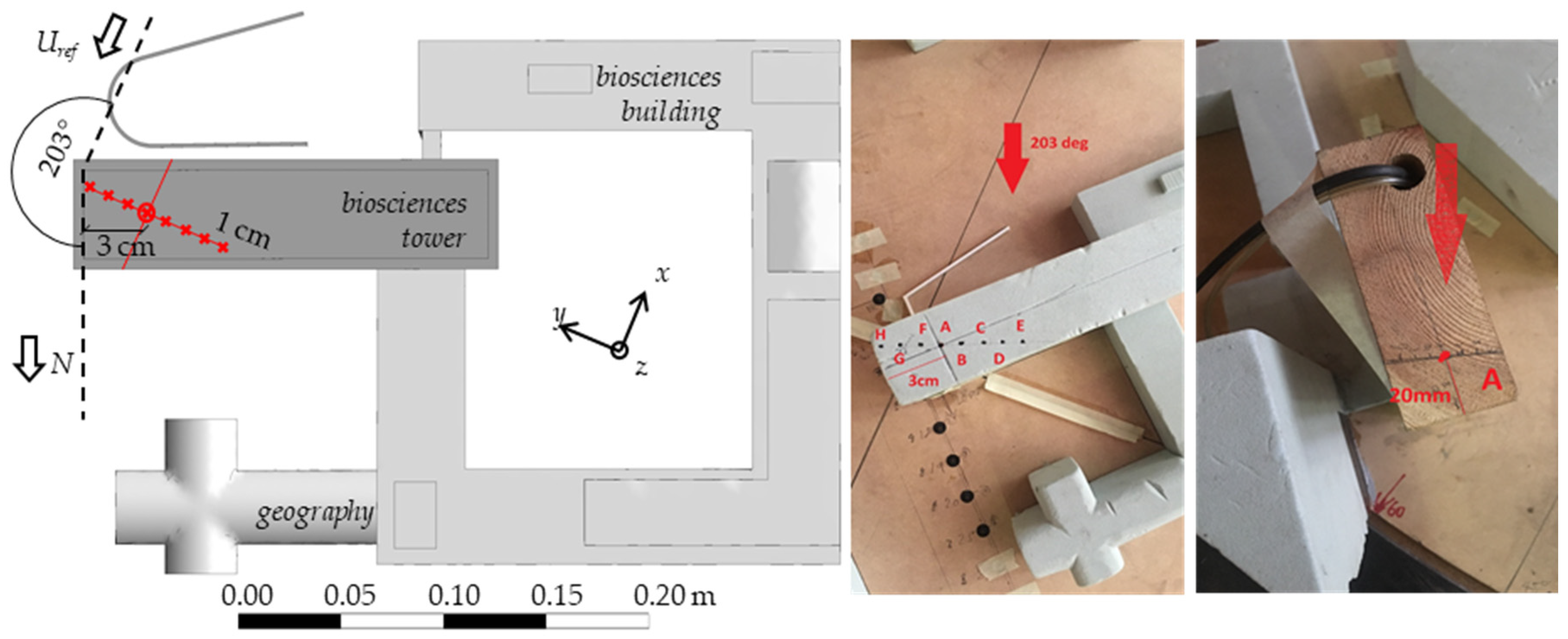
Wind speed measurements are recorded using a Cobra probe, manufactured by Turbulent Flow Instrumentation (TFI) Ltd. (North-East Victoria, Australia). Figure 2 shows the positions where the wind speed profiles above the MT and BB have been measured, i.e., above point A in both cases. In addition, a horizontal profile has been measured above the Biosciences tower, at a height of 4 cm above the roof, equivalent to 12 m in full scale. The cobra probe provides 3-component velocity measurements at a sampling rate of 1250 Hz for the Biosciences tower and 250 Hz for the Muirhead tower. The probe is positioned at the designated measuring points to face the oncoming flow, i.e., in the upstream direction. Wind speeds were recorded for sufficient time, corresponding to at least 1-h in full-scale [26]. This was done for estimating statistically steady values of the targeted wind speed parameters. The output of the Cobra probe is high-pass filtered to eliminate any unwanted noise from the data.
2.3. Numerical Simulation
2.3.1. Computational Domains
The computational domain replicates the geometry and scale of the wind tunnel model. In order to limit computational costs, a thorough optimization of the computational grid size has been performed [21]. While coarsening the mesh is not recommended in literature [6,27], research has started pushing the boundaries of coarse LES to increase its practicality. In cases where a strong validation test case is available, as in this case, the reduction of computational costs might justify the use of a coarser mesh. Nevertheless, extra effort in monitoring the convergence of statistics and the generation of suitable fluctuations at the inlet is an unavoidable requirement. In the present study, the quality of the grid at roof and pedestrian level is optimized with greater refinement than at other locations and results therein are monitored for convergence. Figure 1 shows the computational domain analogous to the experimental setup with two differences. At the outlet surface, an extrusion is added to the domain which is not present in the wind tunnel model, to reduce the blockage of the model with the external boundary, as suggested in BPGs for urban winds modelling [12,28]. At the inlet, the section is elongated to include a portion (~1/3) of the roughness elements, which are used in the wind tunnel to generate the experimental ABL wind profile. The purpose for these elements is to create a turbulent inlet by means of an added geometry to generate turbulence.
For this study, a total of five computational domains have been tested, in order to vary the turbulence of the inflow and to test the impact of neighboring buildings on the flow features above the roof. The computational geometries are reported in Table 1.
The base Case #0 is analogous to computations developed to investigate pedestrian winds in previous research [20], and it represents the validated base geometry with an analogous setup to wind tunnel tests, i.e., with surrounding buildings and presence of roughness cubes of the same size as used in the wind tunnel. In cases #1 and #2 the roughness elements are removed to have a laminar inlet. The surrounding buildings are also removed for case #2. Case #3 proposes the same inlet turbulence as in case #0, without surrounding buildings, while in case #4 the size of roughness cubes is reduced to simulate a different turbulent inlet while retaining the mean wind speed profile simulated in wind tunnel experiments. In all cases the computational domain replicate the geometry of the UoB wind tunnel, i.e., a width of 2 m and a height of 1.90 m, while the fetch length is adapted for each case as shown in Table 1.
2.3.2. Boundary Conditions
The boundary condition for wind tunnel side walls and roof is symmetry, while at the outlet a Neumann condition with a neutral static pressure is imposed, combined with a 1 m elongation of the computational domain to avoid blockage and circulating flow issues. At all other wall boundaries a no slip condition is imposed with a wall function following the Spalding formulation as implemented in Ansys CFX, (Ansys UK Inc., Cambridge, UK) [29,30,31].
As for the inlet, the best fit of the wind tunnel mean wind speed profile is imposed of all simulations with the following power law:
where = 7.8 m/s is the ABL wind speed of the wind tunnel at = 0.65 m, and = 0.3 is the best fitting shear exponent. The mean wind speed is applied to the inlet boundary in order to have the least disruption to the mean wind speed for the different computations, hence testing the impact of different turbulent inlets on the results. The computational domains shown in Table 1 have the scope to fulfil the turbulent inlet boundary condition of LES. The technique lies under the classification of precursor simulation domain for the generation of inlet turbulence for LES [32], i.e., a section of the wind tunnel fetch length is enough to create fluctuations capable of greatly increasing the quality of data in those locations of interest due to the enhanced turbulent inlet. This technique has proven to be successful in improving the precision of numerical data obtained as compared to full scale assessments [33], however it cannot reproduce accurately all the inflow statistics as generated in the wind tunnel as this would entail a more detailed and faithful reproduction of the wind tunnel geometry. Table 1 reports the mean wind speed Uref, the turbulence intensity Iref and the integral length scale Lref as measured at the Biosciences building height, , and the Muirhead tower height, .
2.3.3. Computational Grid
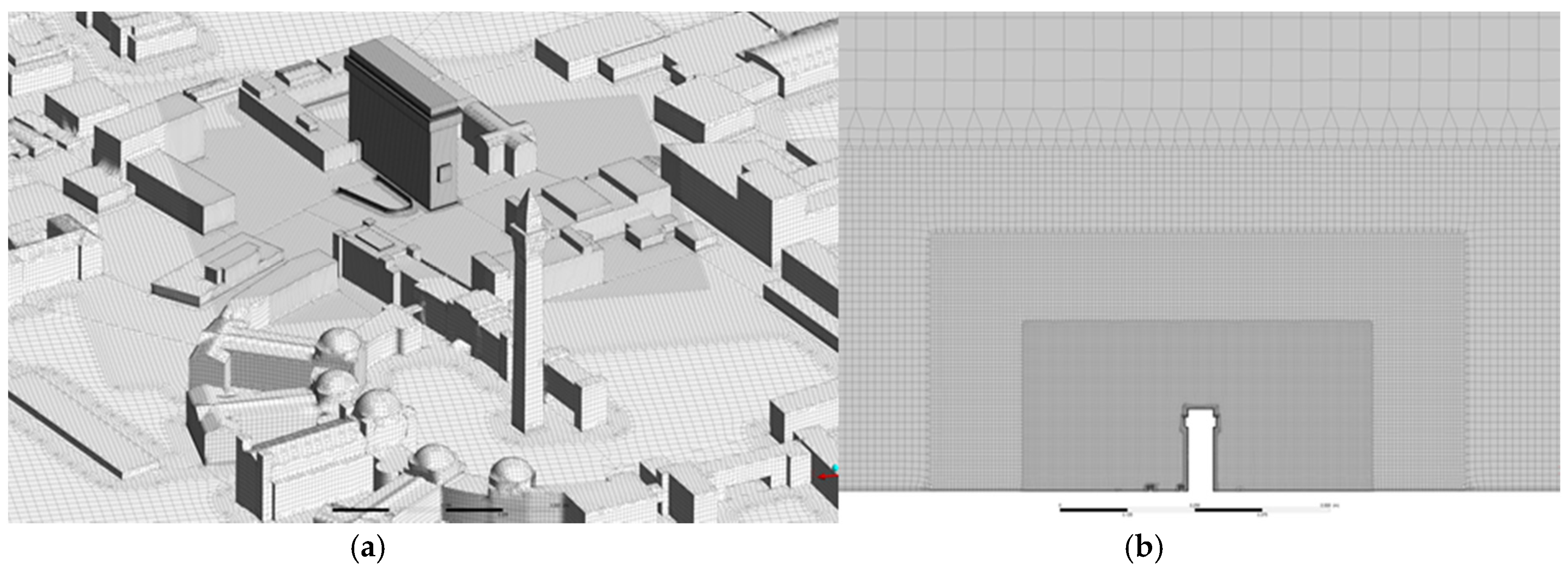
The quality of a LES largely depends on the computational grid and its quality. This work used Numeca International “HEXPRESS™/Hybrid” (Brussels, Belgium) [34] as a 3D mesh generation tool for generating unstructured hexahedral meshes. Amongst the several different meshing utilities available, HEXPRESS/Hybrid is used in this present work due to its ability of meshing large and complex geometries in a fast and easy manner. In addition, the use of this utility for meshing allows for the generation of isotropic and hexahedral dominant meshes. Due to the complexity of the geometries, the meshes did contain few cells of tetrahedral, pyramids and prism types which are all applicable for use in ANSYS CFX. The recommendation for a proper LES would necessitate a mesh with , where is the grid size (also called the cut-off length), and the dissipation length scale of turbulence, which indicates the size of the smallest energy-carrying eddies. As is of the order of 1–10 cm in atmospheric flows [35], this criterion usually results in quasi-DNS (Direct Numerical Simulation), with an exponential rise in computational costs. For this reason, a coarser mesh is chosen , as this is arguably more appealing for industrial practice. The number of cells to build the different computational grids is reported in Table 1.
Figure 3 shows how the coarseness of the grids is obtained for the surface and volume mesh to pursue a cost-effective simulation. The size of the cells increases from ~0.07–0.17 mm close to the Biosciences tower to in the vicinity of surrounding buildings. At further distances the cell size was then gradually increased up to . A boundary layer mesh comprising a minimum of seven prism layers is also introduced at walls. This was done to ascertain that the velocity gradients are resolved precisely while ensuring that the first cell belongs within the Prandtl boundary sub-layer (y+ ~ 5), hence to be compatible with the use of wall functions [21]. Several preliminary RANS have been conducted to obtain the correct cost-effective mesh parameters.
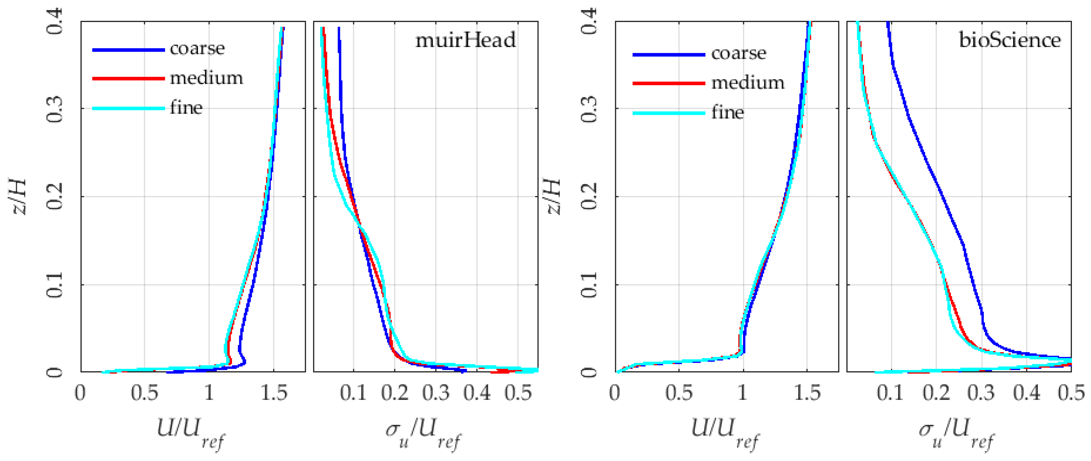
To verify that the computational grid does not affect results, two additional simulations are run for the base case #0 on respectively a coarser and finer grid, with specifications reported in Table 2. Results on both the mean and fluctuating statistics are shown in Figure 4. The coarse grid shows a deviation from the medium and fine grids for the Muirhead tower. Analogously for both towers, the coarse grid overpredicts . However, the medium and fine grids are consistent for both cases.
2.3.4. WM-LES Setup
Using the commercial code Ansys CFX, a set of numerical simulations have been performed on the Linux High Performance Cluster “BlueBEAR” at the University of Birmingham (Birmingham, UK). A total of seven “Haswell” computational nodes were used; over 20 processors, each node has a random-access memory (RAM) of and a clock-time of 4.6 GHz. Using 140 processors per case, the simulations ran for ~10 days to simulate 15 s of LES cases.
Given the coarseness of the mesh and the practical approach, the WM-LES model is chosen, which is a hybrid LES-RANS model where the RANS part is automatically applied at the first cell only. The ratio between LES and RANS exclusively depends on . To elaborate, if , then the WM-LES coincides with standard LES. This model still needs a number of cells similar to traditional LES but avoids all the limitations which may arise due to a too fine/coarse grid when using the classical hybrid Detached Eddy Simulation (DES). More indications on the methodology as coded in Ansys CFX v19.2 are presented in [36]. The Wall-Adaptive Lagrangian-Eulerian (WALE) sub-grid scale (SGS) model has been selected as it allows for a better output for the anisotropy at SGS in wall-bounded flows with respect to the Smagorinsky-Lilly SGS model. This model does not require any extra computations as compared to the Germano SGS model [37]. However, defining a model constant Cw is still required by WALE. For internal flows, it has been suggested that [37]. However, there is evidence that Cw varies greatly with mesh refinement, purporting a lower value better suited for coarser meshes [29,38]. Nevertheless, no specific research on the influence of Cw on realistic urban setups is available to the knowledge of the authors, and works implementing WALE generally follow the recommendations of solver guides as indicated in CFX guidelines seems not to create issues in the validation of results [39,40,41,42]. The solver implements a 2nd order bounded central differencing scheme (CDS) and a 1st order implicit Euler time scheme, as coded in CFX [29]. To ease numerical convergence, the time step has been chosen to fulfil the Courant–Friedrichs–Lewy (CFL) condition, stating that the Courant number , where U, and are the local flow velocity, the local through-flow time, and the local cell size, respectively. For ensuring solution stability, a time step of dt = 0.0005 s is adopted while the resulting Co is demonstrated in Table 2. A sample time of was found to preserve accuracy while enhancing cost-effectiveness.
3. Results
Results in this section are reported at two vertical profiles shown in Figure 2 above point A for the Biosciences building and the Muirhead tower, and a horizontal profile. Experimental measurements have been conducted in the same positions and are compared to results for case #0.
3.1. Inlet Turbulence
The characteristics of the inlet wind profile obtained for the different computational domains is shown in Figure 5, while turbulent fluxes are shown in Figure 6.
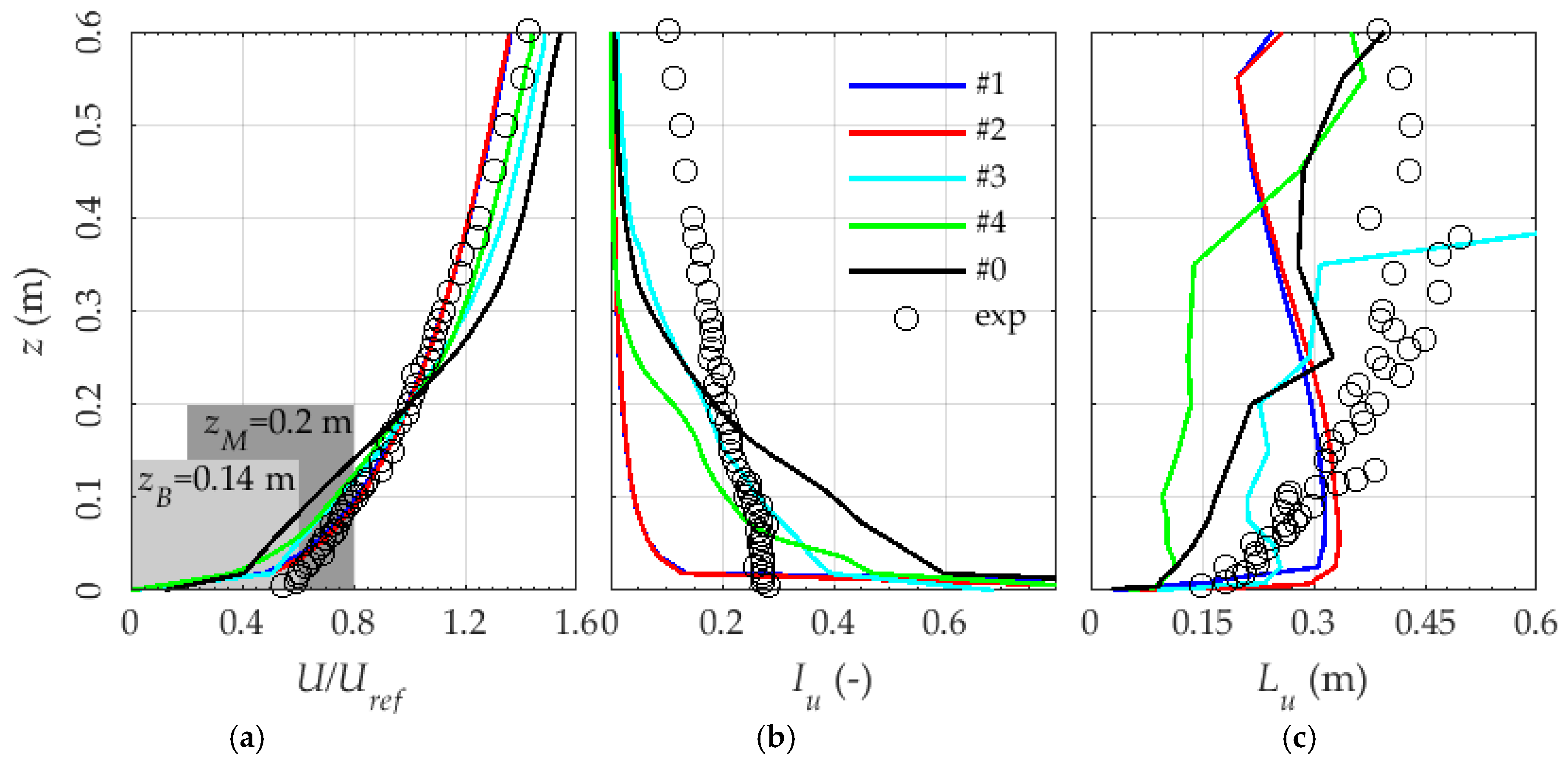
The computational profile is measured as indicated in Table 1, 1 m upstream of the Biosciences Building, downstream of the roughness cubes of the wind tunnel domain, if present. The reference wind tunnel profile is measured instead at the same position 1 m upstream of the test platform center in the absence of the model campus. In fact, a deviation for the mean wind speed profile is noticeable for cases #0, #3 and #4, and this is due to the wake that develops downstream of the roughness geometry used to generate turbulence. The turbulence intensity profile shows how cases #0 and #3 match the experimental profile at z ~ 0.2 m, while case #4 expectedly generates a different turbulence intensity due to the different roughness elements, and cases #1 and #2 have a low turbulence intensity <5%. The turbulence intensity distribution is in all cases inaccurate and this is due to the lack of a synthetic boundary conditions or a larger portion of the wind tunnel reproducing the turbulence at the inflow. Arguably the match is comparable at the heights of both high-rise buildings as indicated in Figure 5. A larger deviation from the experimental results is also noticeable for the integral length scale, and at z ~ 0.2 m for cases #0 and #3, which is lower than the experimental Lu ~ 0.4 m. The lack of spires in the computations accounts for low turbulence at z > 0.3 m.
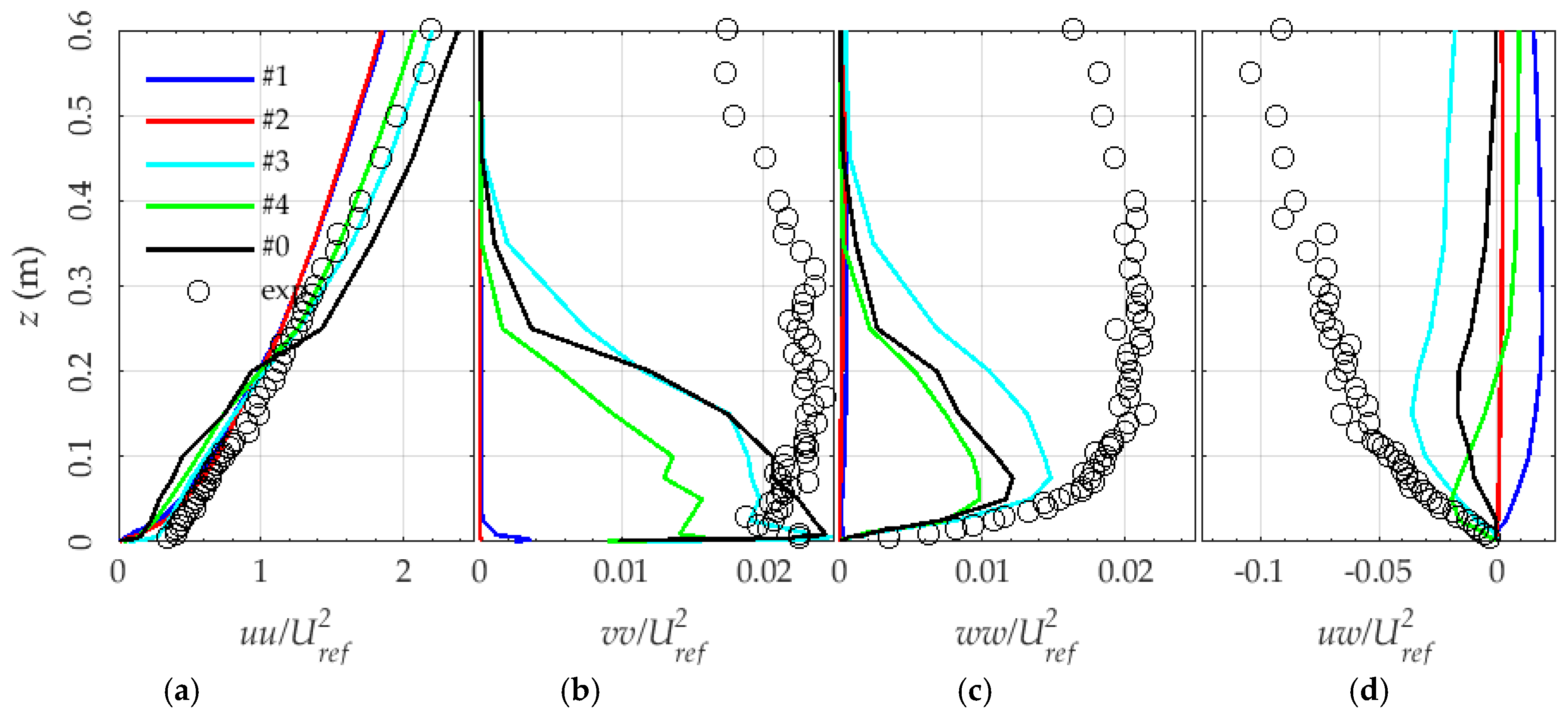
Figure 6 shows the turbulence fluxes uu, vv, ww and uw. These highlight the influence of the surrounding buildings on the wind profile. The vertical fluxes ww and uw show that the blockage of the buildings causes case #3 to have a stronger updraft than case #0. As for the symmetrical fluxes uu and vv, the presence of buildings does not affect the turbulent inflow. The inflow is analogous to the experimental wind profile up to z ~ 0.1 m for vv, ww and uw, to then deviate significantly due to the lack of turbulence at z > 3 m. The symmetrical flux uu deviates significantly in the portion z < 0.2 m for case #0, while cases #3 and #4 are weakly affected. This could depend on the effect of the blockage of the campus modelling all the buildings. Notably, the experimental profile is obtained without the presence of the models, hence the stretch of turbulence due to blockage which is present in numerical cases might be the cause for the mismatch showed in Figure 6, causing the flow patterns of Table 3.
3.2. Flow Pattern
Table 3 shows the flow pattern obtained with the different computational domains in terms of mean wind speed U, standard deviation and instantaneous wind speed u.
The effect of the turbulent inlet variation is noticeable in terms of extent of the separation region. In case #0, the mean wind speed shows that the recirculation region above the roof is limited to z ~ 0.15 zB, while the wake core is located at a distance of ~0.5 zB from the building. This distance is found to depend on the presence of surrounding buildings, as it increases to ~zB for cases #2 and #3 regardless of the turbulence at the inflow. As regards the turbulent environment above the roof, the absence of turbulence at the inlet strongly underestimates the turbulence at the roof and its extent. In fact, a much smaller shear region is found in the absence of turbulence, with an extent of ~0.1 zB.
The instantaneous flow also shows the tendency for the wake to recover. In cases #0, #3, and #4 the wake starts to dissipate 1.5 zB downstream of the building, while cases #1 and #2 only show a dissipation at ~3 zB, regardless of the presence of surrounding buildings.
3.3. Mean Wind Speed
Both the horizontal wind speed and the vertical velocity are reported and compared with the experimental results for the different cases. Previous research has shown that LES has a comparable performance to RANS in predicting the mean wind speed over both buildings [21]. LES is found to generally improve accuracy, especially with regards to the separated flow region. A mismatch in the turbulent inlet as modelled for a setup analogous to case #0 is found to have a limited effect on accuracy. This might explain why RANS works well in predicting the mean wind speed, i.e., the physical behavior is mostly influenced by the building itself and not the surrounding flow. However, to be of use to urban wind energy applications, the mean wind speed is not exhaustive to predict the feasibility of a device positioning, e.g., from U one cannot estimate the annual energy production.
Figure 7 shows the wind speed profiles measured above both towers.
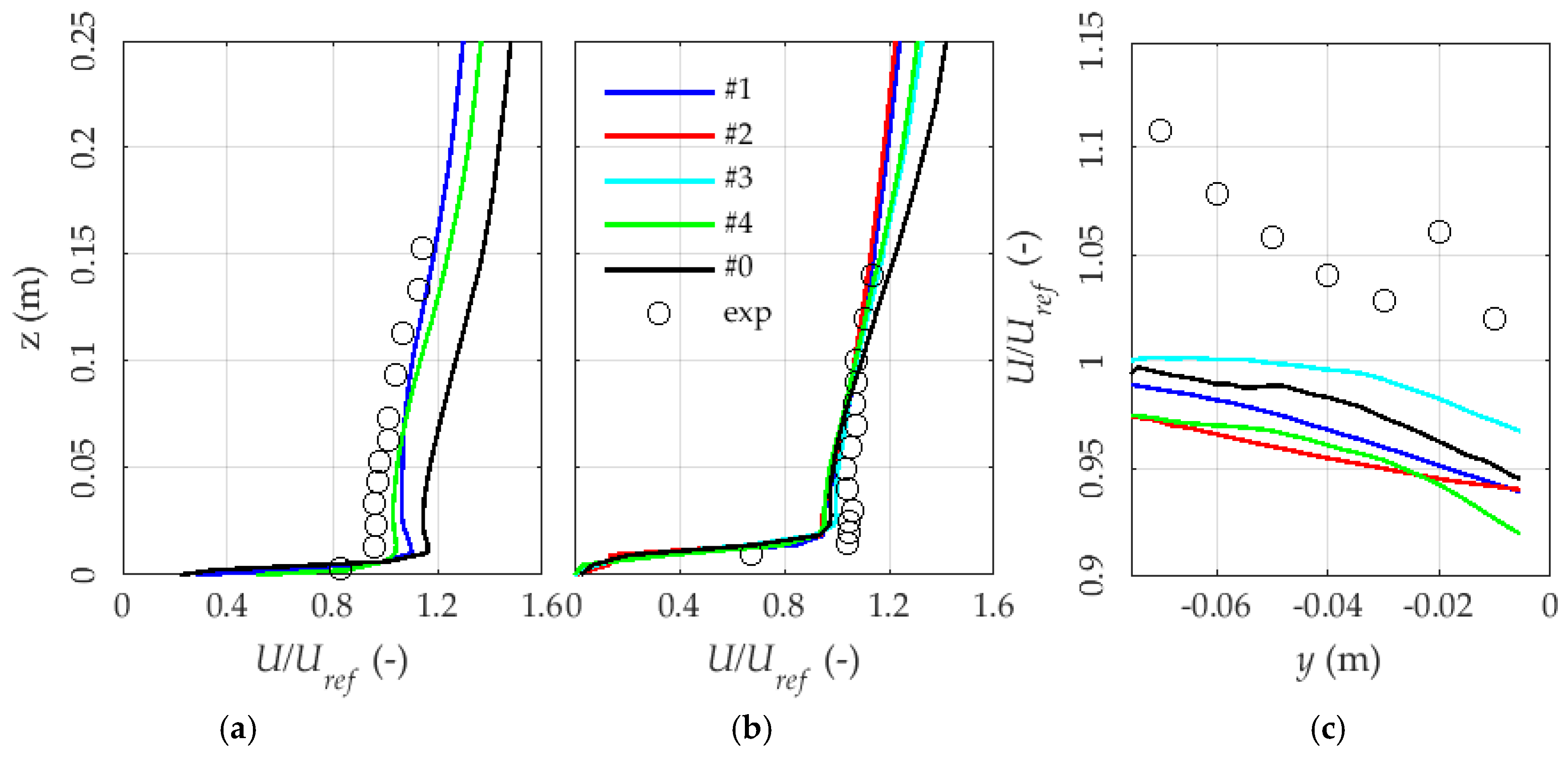
For the Muirhead tower, only cases #1 and #4 are shown, as in cases #2 and #3 buildings surrounding the Biosciences tower are not modelled, including the Muirhead tower itself. The LES predicts accurately both U and W, with a deviation from experimental results of less than ~2%. For z > 0.1 m above the roof, results deviate by ~10% for the BB. This deviation might occur due to the positions of the models. In fact, the MT is facing directly the inflow from the wind tunnel, while the BB is right in the middle of the model and hence affected by the signature turbulence and wakes coming from surrounding buildings.
This might depend on the mismatch in the choice of Uref and the profile over the Muirhead Tower. In fact, this position is heavily affected by the mismatch of inlet boundary conditions as shown in Figure 5, and therefore different velocities are found above the roof.
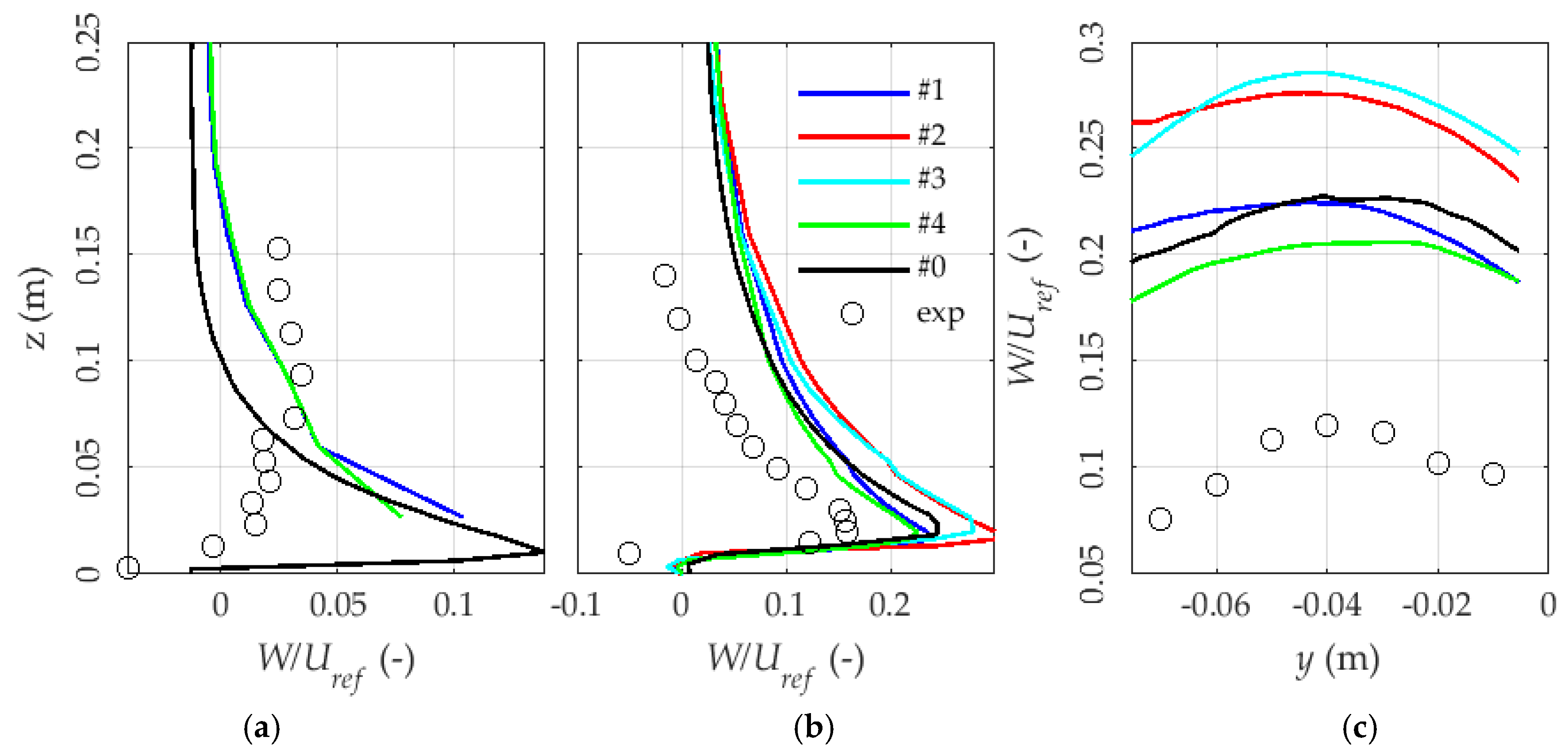
Figure 8 shows the vertical velocity profiles. The mismatch with the experimental case is evident for the Muirhead tower, where significant differences are present in the geometry due to its position at the edge of the turntable. In general, LES overpredicts W and this is consistent for all cases, suggesting a possible significant role for the effect of the blockage of the computational domain. In general isolated cases #1 and #3 have a higher vertical component.
3.4. Turbulence Intensity
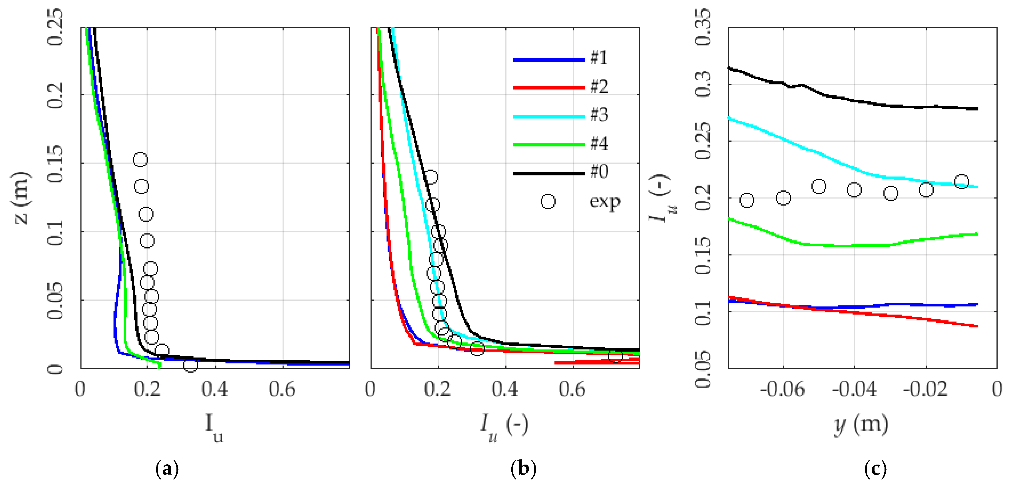
The mean wind speed U and the standard deviation of the horizontal wind speed and vertical velocity are used to calculate the turbulence intensity. Figure 9 shows the longitudinal turbulence intensity Iu.
Above the Muirhead tower, all cases tend to underestimate Iu. The mismatch can be attributed to the inlet turbulence of the cut wind tunnel domain. The portion of the fetch length modelled is enough to guarantee a match with the experimental wind conditions up to z ~ 0.2 m from the ground, however at the roof height, a strong mismatch is present, affecting the turbulence intensity as predicted. The mismatch of the Biosciences building is less pronounced. While cases #1 and #2 strongly underestimate the intensity due to the absence of turbulence at the inflow, cases#0 and #3 are quite accurate, within ~20% compared to experimental measurements. Case #4 shows the effect of a slightly lower inlet turbulence intensity affecting directly the local profile. The effect of the surrounding buildings seems not to be affecting the turbulence intensity prediction, with a weak decrease in the predicted Iu in the absence of surrounding buildings.
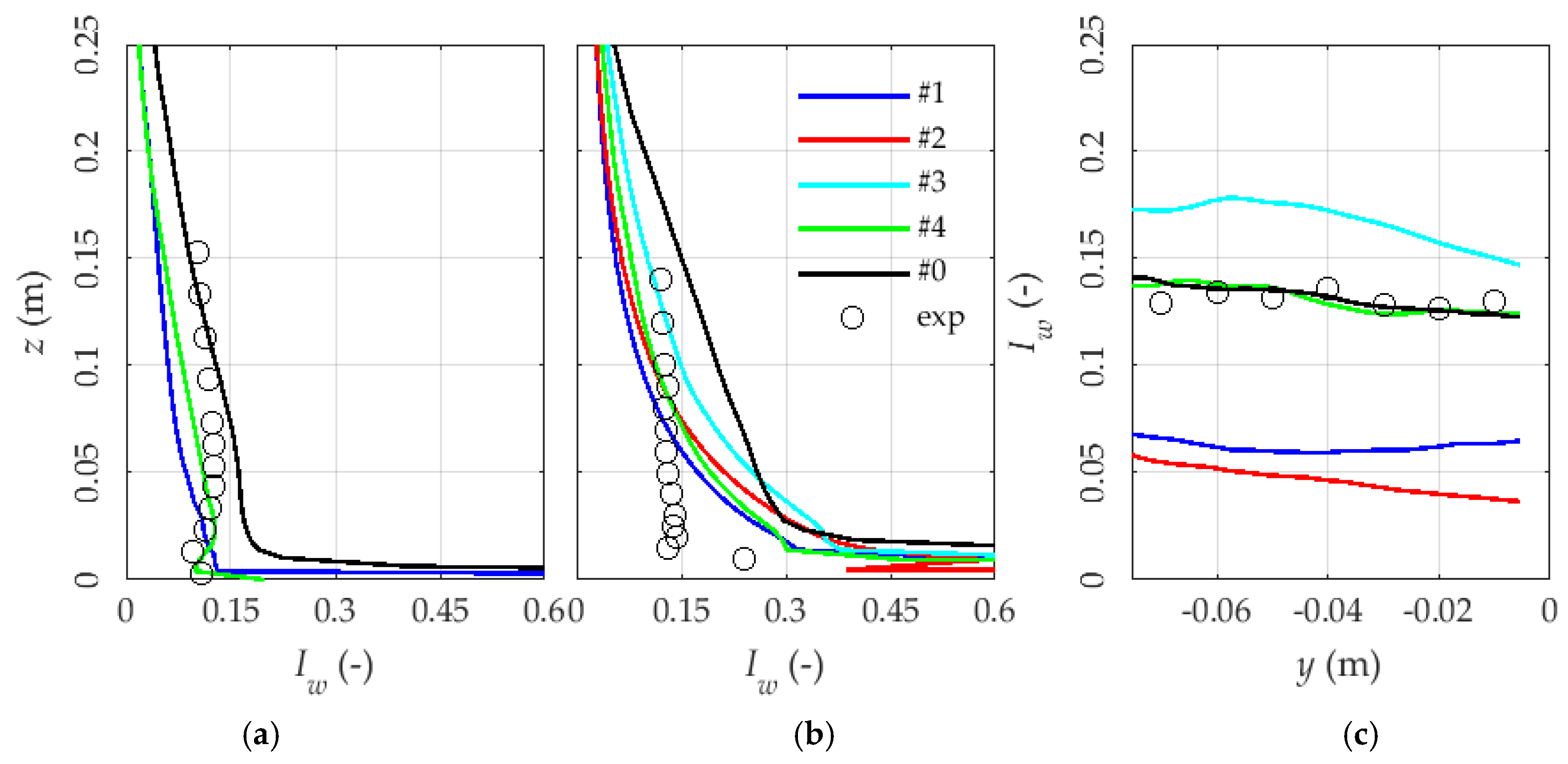
Figure 10 shows the vertical turbulence intensity, for which the mismatch is analogous to that shown in Figure 9 for Iu. However, the absence of turbulence at the inlet seems only to affect weakly the vertical intensity. The distribution of Iu and Iw is quite different from experimental data, suggesting that a mismatch in the turbulence intensity of the inflow affects the turbulence intensity above the roof significantly. In general, a lower inflow turbulence causes a lower turbulence intensity to be predicted. The mismatch of case #0 is larger than other cases, although the simulation resembles the experimental setup. This might be due to the inflow wind speed profile. Nevertheless, all cases tend to overestimate the turbulence intensity above the roof. In view of urban wind energy, this might be considered a useful economical way of identifying regions of high and low turbulence above the roof, in the preliminary phases of design where wind tunnel tests might not yet be available.
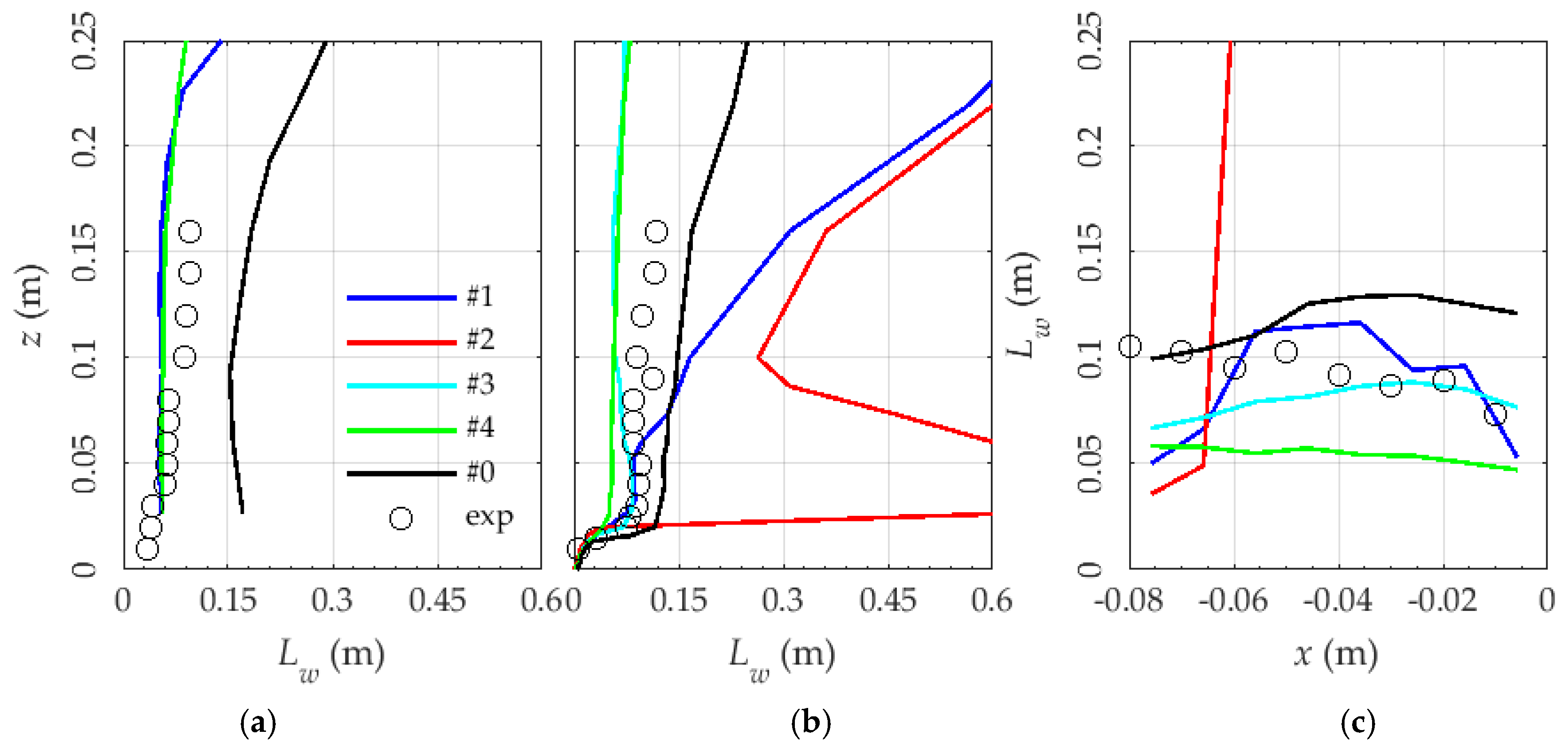
3.5. Integral Length Scale of Turbulence
The integral length scale of turbulence is computed from the autocorrelation coefficient with the use of the Wiener-Khintchine theorem and the Taylor hypothesis:
where U is the mean wind speed, is the autocorrelation coefficient for the wind speed u, is the lag time and is defined such that .
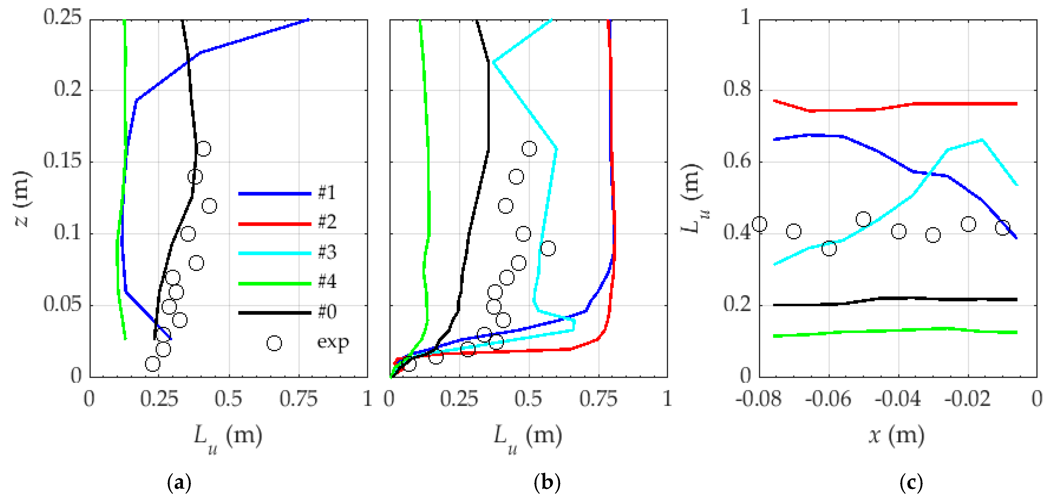
Figure 11 shows the integral length scale of turbulence of the wind speed u. Lu is sensitive to variations of inlet turbulence, as shown for the Muirhead tower. As for the Biosciences building, the presence of the building increases the integral scale with respect to the inflow by ~20%, and cases #0 and #3 are able to predict this, suggesting that surrounding buildings do not affect the integral length scale above the roof of tall buildings. The horizontal profile also shows that the length scale is predicted closely by case #3, which has a closer match of turbulence statistics to the inflow.
The vertical length scale shows how critical is the introduction of turbulence at the inflow in LES. Figure 12 shows that the turbulent inflow improves accuracy significantly.
Little difference occurs because of the existence of surrounding buildings, especially closer to the roof, where all cases predict the vertical length scale accurately with the notable exception of case #1. It can be stated that the presence of turbulence is essential to model the integral length scale, while it is not important to accurately reproduce turbulence at the inflow.
In general, at z < 0.025 m the match with experimental values is closer than at other heights, suggesting that the behavior is commanded by the leading edge vortices only in the separated flow region. The prediction of coherent structures above high-rises requires a careful modelling of the inflow in terms of turbulence characteristics.
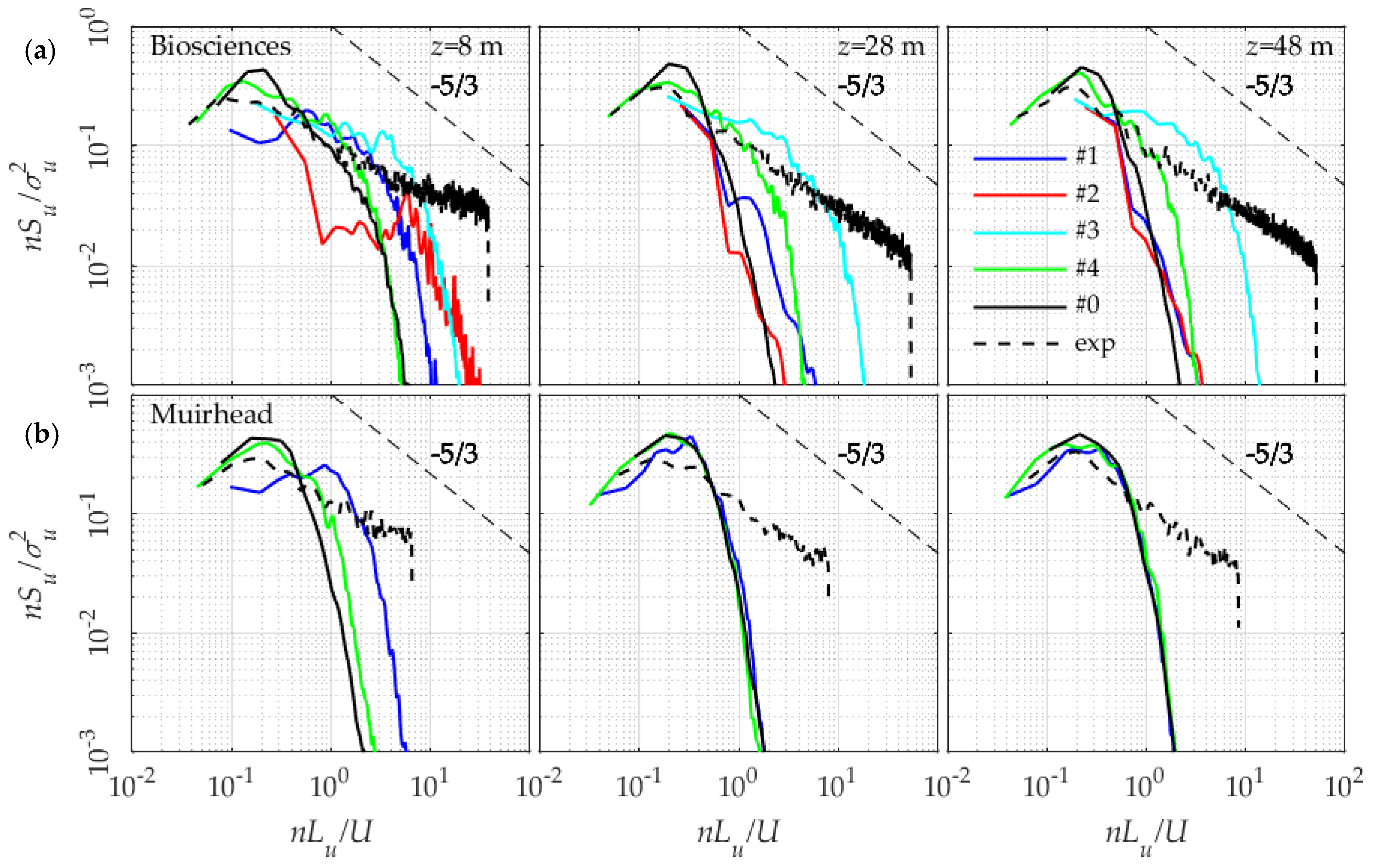
3.6. Energy Spectra
The energy spectra of the wind speed are shown in Figure 13 for both towers at different heights. Energy spectra are a useful way to determine the amount of turbulent energy solved in LES.
In this case, the optimization of the computational grid does not impair the spectra, as a significant portion of the experimental frequencies is resolved. In fact, close to the roof, a close match with experimental spectra is obtained up to a reduced frequency of ~10, while at higher quotes the results are affected by the coarsening of the mesh further from the roof. LES is able to predict a significant amount of information using a coarse mesh, while inflow turbulence only affects the spectra at heights z > 10 m. In fact, case #2 is able to describe the behavior analogously to other cases at z = 8 m. As for the Muirhead tower, the presence or absence of the turbulence inlet seems not to affect the prediction, suggesting that a sufficient modelling of the area surrounding the building of interest might positively influence results, without an accurate inflow profile. Figure 13 also shows that the integral length scale is well predicted and weakly affected by the inflow turbulence. Case #3 shows in the upper row of Figure 13, that surrounding buildings play an important role in the energy cascade for z > 10 m.
3.7. Gust Wind Speed
The estimation of the gust speed ug calculated using the quantile of the velocity signals can give further insights on the prediction of the different setups of extreme events. Several methods can be used to calculate ug. In this work, the moving average technique is used.
Figure 14 shows the 90th quantile of the horizontal wind speed . The introduction of turbulence is in this case essential as cases #1 and #2 strongly underestimate the gust wind speed. The Biosciences building shows that LES underpredicts ug by ~10%.While this might be affected from the choice of Uref, a role could be played by the shorter sample time Tg used to reduce computational costs compared to the experimental sample time. While this issue can be easily resolved increasing Tg, present results show that a variation in the turbulent inflow setup seems not to affect extremal statistics. In fact, case #0 and case #3 show an analogous behavior, closest to experimentally obtained data, while case #4 shows that a reduced turbulence intensity is responsible for a reduced gustiness, which is consistent with results available for pedestrian winds [20]. Interestingly, the presence of surrounding buildings seems not to have an effect on ug, suggesting that extreme winds are highly dependent on the local features of the flow around the high-rise building. The lack of turbulence in the inflow affects gustiness significantly.
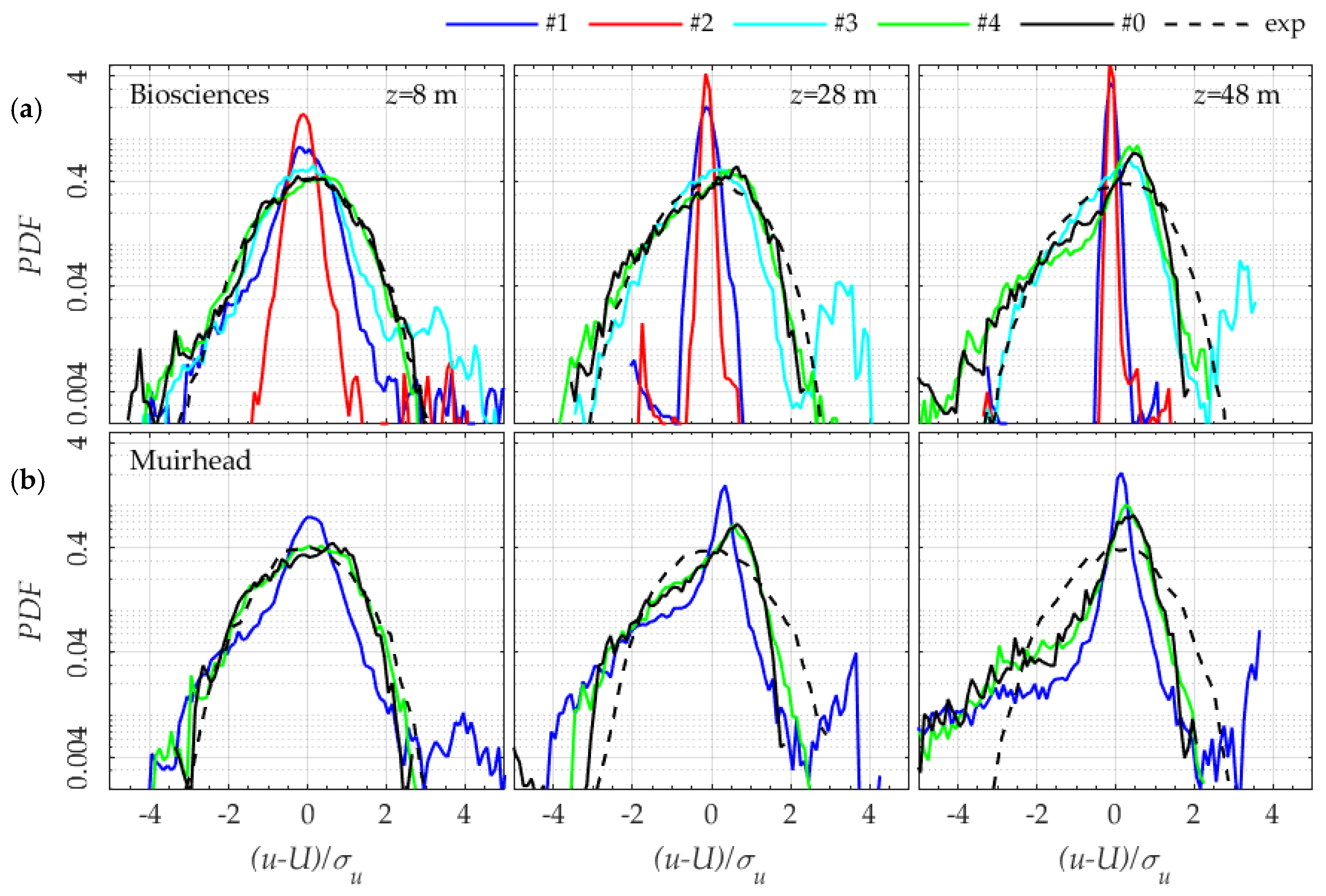
3.8. Probability Density Function
For estimating the potential yield of wind energy applications, the probability density function (PDF) of the wind resource are an extremely useful result to convert the numerically resolved flow field into an annual energy production estimation, as done for standard wind farm plans. In addition, it helps plan and predict uncertainty for wind energy [43]. PDFs can also complement information on the extremal statistics behavior shown in Figure 14.
Figure 15 shows the (PDF for the horizontal wind speed following the same heights shown in Figure 13 for the energy spectra. PDFs confirm that at lower heights , the influence of the turbulence inflow is rather limited on the accuracy of results, if a sufficiently large area is modelled around the building of interest. Besides the mismatch of turbulence characteristics, the prediction of LES is very accurate for the skewness for both towers, with a mismatch for the Muirhead tower, where the flow is positively skewed at z > 10 m. The positive skewness might occur due to its position at the edge of the test-section, hence in an area less detailed compared to the Biosciences building. However, a light positive skewness can be also noticed from experimental measurements, which might reflect the way the turbulent inflow is generated from roughness elements and their wakes.
For the BB another issue might be noted around the behavior of higher order moments close to the roof, as noticeable from the PDF and not shown for brevity. In fact, kurtosis becomes strongly positive, while skewness remains positive throughout the profile. This is indicative of the highly vorticity of the behavior inside the separation bubble, which experiences bursting and vorticity which causes high velocities to be more likely than slow ones in a region with low mean velocity.
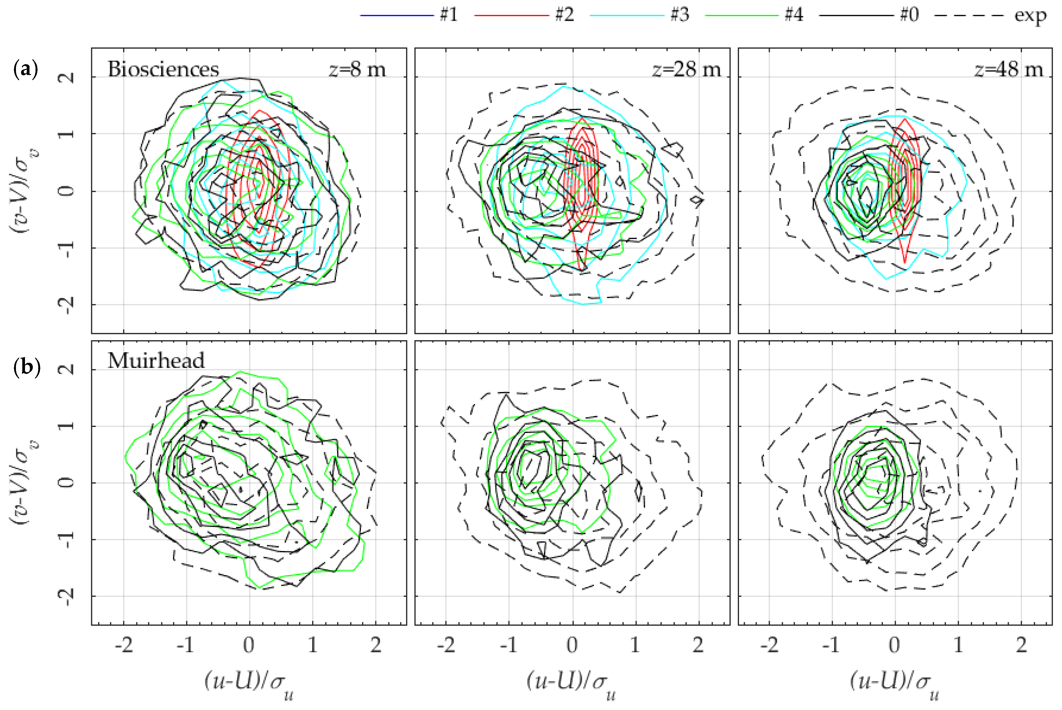
3.9. Quadrant Analysis
Figure 16 shows the joint PDFs (JPDF), which can also give a deep insight on the behavior of extremal statistics and how they behave in three-dimensional flows.
The quadrant analysis is conducted through the JPDFs for the longitudinal and transversal velocities u and v. u is here to be intended as the wind-wise velocity component, unlike in the rest of the paper where it represents the horizontal wind speed.
The first result from Figure 16 is to notice how LES closely predicts the tridimensional behavior at all heights, having the JPDF a similar shape in cases #0, #3 and #4 which all model turbulence at the inflow. At z = 8 m all cases predict the turbulence behavior with the exception of case #1, while at other heights it is evident how important the introduction of turbulence inflow is for the prediction, regardless of the presence of surrounding buildings, as cases #1 and #2 yield an unphysical behavior for both BB and MT. As for the MT, case #4 shows the effect of a different turbulence intensity, as the JPDF shrinks around the center of the graph compared to experimental results and case #0.
4. Discussion and Conclusions
Results seem to support the hypothesis that the above roof flow can be divided into regions, depending on their sensitiveness to the turbulent inflow characteristics. At z~8 m, a region of the flow is found which is rather insensitive to the inflow or the presence of surrounding buildings, hence uniquely affected by the immediate surrounding geometry, while being rather insensitive to the global wind profile. At higher quotes a region of the flow sensitive to the inflow is found, with some statistics insensitive to the turbulence (such as the turbulence intensity) and some other rather insensitive (such as the Integral length scale).
This paper gives novel results on the effect of the several factors that affect the flow pattern in realistic urban environments, in contrast with ideal cases such as those investigated so far in literature. The paper has investigated how introducing a variability of the inflow conditions and the surroundings affects the local flow pattern. In general, in a realistic urban environment, the flow features have the following properties:
- The randomness of the wind conditions implies a random angle of attack and asymmetry of the geometry of the high-rise building;
- The roughness distribution around the high-rise, which fluctuates significantly depending on the immediate surroundings of the building and the built environment around.
Results show that the prediction of the turbulence in an urban environment is a rather challenging task both for wind tunnel and numerical tests.
The interaction between inlet scales as predicted numerically and the buildings might also be an effect of the meshing strategy, which balances the cost of the simulation with the size of the mesh, resulting in a cell-size of ~10 m in the freestream region above the UoB campus. Modelling the correct inlet turbulence is therefore deemed necessary to have a correct assessment of the flow pattern above the buildings.
The numerical setup prompts a further observation. The unstructured coarse grid used for this study is normally a risky choice for LES, as a broad band of frequencies is demanded to the SGS model of choice. However, refining the mesh in those regions of interest, as in the present study, paying attention to the y+ value and the convergence of results and provided a good validation test-case is available, shows how the local features of the flow field in the urban settings are mostly insensitive to the surrounding flow fields. This could open up the possibility of implementing coarse high-fidelity simulations to aid wind tunnel tests in increasing the prediction accuracy of the flow features of the roof region. While LES purists might be terrified from such a conclusion, the clear benefits over RANS in terms of performance, accuracy, reliability and the improved amount of information, justifies in the authors’ view the present LES setup for practical urban flow applications.
The roof-level flow on high-rise buildings is heavily influenced by the turbulence at the inlet. In fact, it could be possible that a careful modelling of the turbulent inlet structures at the inflow might substitute the necessity of a finer mesh to improve accuracy and reliability of results, which is indeed interesting in the view of using LES for practical applications, as done in this study.
A further reflection on the behavior of the flow that develops above the roofs of high-rise structures such as buildings is necessary if the positioning of wind turbines is looked at. The mere match of the mean velocity inlet profile is not a guarantee for a careful prediction of turbulence statistics, in particular the integral length scale. Experimental data confirms that turbulence intensities greater than 20% are to be expected in a region above the high-rise building as high as the building itself, prompting doubts about results published in literature so far considering RANS as a suitable choice to assess the turbulent environment and assess the positioning strategy of wind turbines based on turbulence intensity [4,21].
Results also confirms that LES is suitable to model a wide range of statistics and competes with wind tunnel testing in accuracy, if a correct balance between the cost-effectiveness of simulations and the provision of suitable inlet turbulence characteristics.
As for the role of the inflow variability the following conclusions can be drawn:
- Modelling inflow turbulence is essential to the accuracy of the simulation;
- Matching the real inflow turbulence characteristics is not of utmost importance to obtain an acceptable description of the local flow, especially close to the building surfaces;
- Close to the roof, the behavior is only affected by the leading edge generated coherent structures, and not by the inflow characteristics;
- The turbulence intensity is the most sensitive parameter to differences in the turbulent inflow;
- The integral length scale is also sensitive, but to a lesser extent;
- The mean wind speed is rather insensitive to variations in the turbulent inlet;
- Surrounding buildings also need to be modelled, but their role is limited in generating local turbulence. Hence, if a turbulent inlet is present, isolated buildings can also be modelled to obtain a reasonable estimate of the wind energy resource;
- Vice versa, if a turbulent inflow is absent, modelling surrounding buildings improves accuracy due to the generation of local turbulence. However, a larger area should to be modelled, as shown for the Muirhead Tower in the present study, placed downstream of the testing platform and showing in general a better match in absence of turbulence than found for the Biosciences Tower.
- The wake of modelled buildings is heavily affected by inflow turbulence, while it looks insensitive to the presence of surrounding buildings, suggesting wakes depend mostly on the inflow rather than the local geometric and flow features.
Author Contributions
Conceptualization, G.V.; methodology, G.V. and S.A.H.; validation, G.V.; formal analysis, G.V.; investigation, G.V. and S.A.H.; resources, H.H. and C.B.; data curation, G.V. and S.S.; writing—original draft preparation, G.V.; writing—review and editing, G.V. and S.A.H.; supervision, H.H., C.B. and S.S. All authors have read and agreed to the published version of the manuscript.
Funding
The support of the European Commission’s Framework Program “Horizon 2020” through the Marie Skłodowska-Curie Innovative Training Networks (ITN) “AEOLUS4FUTURE—Efficient harvesting of the wind energy” (H2020-MSCA-ITN-2014: Grant agreement no. 643167) is acknowledged together with the plethora of data and expertise provided by the COST Action TU1804 WINERCOST—“Wind Energy to enhance the concept of Smart cities” The research framework from which this work has originated from has received funding from the UK Engineering and Physical Science Research Council, which funded the original research on “The safety of pedestrians, cyclists and motor vehicles in highly turbulent urban wind flows” under grant number EP/ M012581/1.
Acknowledgments
The authors thank Zhenru Shu for providing the experimental wind tunnel data used to validate the present numerical results. Michael Jesson is also thanked for making available full-scale field test results.
Conflicts of Interest
The authors declare no conflict of interest. The funders had no role in the design of the study; in the collection, analyses, or interpretation of data; in the writing of the manuscript, or in the decision to publish the results.
References
- Evans, B.; Parks, J.; Theobald, K. Urban wind power and the private sector: Community benefits, social acceptance and public engagement. J. Environ. Plan. Manag. 2011, 54, 227–244. [Google Scholar] [CrossRef] [Green Version]
- Stathopoulos, T.; Alrawashdeh, H. Urban Wind Energy: A Wind Engineering and Wind Energy Cross-Roads; Springer: Cham, Switzerland, 2019; pp. 3–16. [Google Scholar]
- Stathopoulos, T.; Alrawashdeh, H.; Al-Quraan, A.; Blocken, B.; Dilimulati, A.; Paraschivoiu, M.; Pilay, P. Urban wind energy: Some views on potential and challenges. J. Wind Eng. Ind. Aerodyn. 2018, 179, 146–157. [Google Scholar] [CrossRef]
- Toja-Silva, F.; Kono, T.; Peralta, C.; Lopez-Garcia, O.; Chen, J. A review of computational fluid dynamics (CFD) simulations of the wind flow around buildings for urban wind energy exploitation. J. Wind Eng. Ind. Aerodyn. 2018, 180, 66–87. [Google Scholar] [CrossRef]
- Millward-Hopkins, J.T.T.; Tomlin, A.S.S.; Ma, L.; Ingham, D.; Pourkashanian, M. The predictability of above roof wind resource in the urban roughness sublayer. Wind Energy 2012, 15, 225–243. [Google Scholar] [CrossRef]
- Blocken, B. LES over RANS in building simulation for outdoor and indoor applications: A foregone conclusion? Build. Simul. 2018, 11, 821–870. [Google Scholar] [CrossRef] [Green Version]
- Bontempo, R.; Manna, M. Highly accurate error estimate of the momentum theory as applied to wind turbines. Wind Energy 2017. [Google Scholar] [CrossRef]
- Micallef, D.; van Bussel, G. A Review of Urban Wind Energy Research: Aerodynamics and Other Challenges. Energies 2018, 11, 2204. [Google Scholar] [CrossRef] [Green Version]
- Tolias, I.C.; Koutsourakis, N.; Hertwig, D.; Efthimiou, G.C.; Venetsanos, A.G.; Bartzis, J.G. Large Eddy Simulation study on the structure of turbulent flow in a complex city. J. Wind Eng. Ind. Aerodyn. 2018, 177, 101–116. [Google Scholar] [CrossRef] [Green Version]
- Hertwig, D.; Patnaik, G.; Leitl, B. LES validation of urban flow, part II: Eddy statistics and flow structures. Environ. Fluid Mech. 2017, 17, 551–578. [Google Scholar] [CrossRef] [Green Version]
- Šarkić Glumac, A.; Hemida, H.; Höffer, R. Wind energy potential above a high-rise building influenced by neighboring buildings: An experimental investigation. J. Wind Eng. Ind. Aerodyn. 2018, 175, 32–42. [Google Scholar] [CrossRef] [Green Version]
- Franke, J.; Hellsten, A.; Schlunzen, K.H.; Carissimo, B. The COST 732 Best Practice Guideline for CFD simulation of flows in the urban environment: A summary. Int. J. Environ. Pollut. 2011, 44, 419. [Google Scholar] [CrossRef]
- Kubota, T.; Miura, M.; Tominaga, Y.; Mochida, A. Wind tunnel tests on the relationship between building density and pedestrian-level wind velocity: Development of guidelines for realizing acceptable wind environment in residential neighborhoods. Build. Environ. 2008, 43, 1699–1708. [Google Scholar] [CrossRef]
- Tsang, C.W.; Kwok, K.C.S.; Hitchcock, P.A. Wind tunnel study of pedestrian level wind environment around tall buildings: Effects of building dimensions, separation and podium. Build. Environ. 2012, 49, 167–181. [Google Scholar] [CrossRef]
- Vita, G.; Šarkić-Glumac, A.; Hemida, H.; Salvadori, S.; Baniotopoulos, C. On the Wind Energy Resource Above High-Rise Buildings. Energies 2020, 13, 3641. [Google Scholar] [CrossRef]
- Hemida, H.; Šarkic Glumac, A.; Vita, G.; Kostadinović Vranešević, K.; Höffer, R. On the flow over high-rise building for wind energy harvesting: An experimental investigation of wind speed and surface pressure. Appl. Sci. 2020, 5283, In review. [Google Scholar] [CrossRef]
- Kanda, M. Progress in Urban Meteorology: A Review. J. Meteorol. Soc. Jpn. 2007, 85B, 363–383. [Google Scholar] [CrossRef]
- Toparlar, Y.; Blocken, B.; Maiheu, B.; van Heijst, G.J.F. A review on the CFD analysis of urban microclimate. Renew. Sustain. Energy Rev. 2017, 80, 1613–1640. [Google Scholar] [CrossRef]
- Yoshie, R.; Mochida, A.; Tominaga, Y.; Kataoka, H.; Harimoto, K.; Nozu, T.; Shirasawa, T. Cooperative project for CFD prediction of pedestrian wind environment in the Architectural Institute of Japan. J. Wind Eng. Ind. Aerodyn. 2007, 95, 1551–1578. [Google Scholar] [CrossRef]
- Vita, G.; Shu, Z.; Jesson, M.; Quinn, A.; Hemida, H.; Sterling, M.; Baker, C. On the assessment of pedestrian distress in urban winds. J. Wind Eng. Ind. Aerodyn. 2020, 203, 104200. [Google Scholar] [CrossRef]
- Vita, G. The Effect of Turbulence in the Built Environment on Wind Turbine Aerodynamics; University of Birmingham: Birmingham, UK, 2020. [Google Scholar]
- Ricci, A.; Kalkman, I.; Blocken, B.; Burlando, M.; Freda, A.; Repetto, M.P. Large-scale forcing effects on wind flows in the urban canopy: Impact of inflow conditions. Sustain. Cities Soc. 2018, 42, 593–610. [Google Scholar] [CrossRef]
- Tominaga, Y.; Mochida, A.; Shirasawa, T.; Yoshie, R.; Kataoka, H.; Harimoto, K.; Nozu, T. Cross Comparisons of CFD Results of Wind Environment at Pedestrian Level around a High-rise Building and within a Building Complex. J. Asian Archit. Build. Eng. 2004, 3, 63–70. [Google Scholar] [CrossRef]
- Vasaturo, R.; Kalkman, I.; Blocken, B.J.E.; van Wesemael, P.J.V.J.V. Large eddy simulation of the neutral atmospheric boundary layer: Performance evaluation of three inflow methods for terrains with different roughness. J. Wind Eng. Ind. Aerodyn. 2018, 173, 241–261. [Google Scholar] [CrossRef]
- Ricci, A.; Burlando, M.; Repetto, M.P.; Blocken, B. Simulation of urban boundary and canopy layer flows in port areas induced by different marine boundary layer inflow conditions. Sci. Total Environ. 2019. [Google Scholar] [CrossRef] [PubMed]
- ASCE Wind tunnel testing for buildings and other structures. ASCE Stand. 2012, 1–54. [CrossRef]
- Hanjalic, K. Will RANS Survive LES? A View of Perspectives. J. Fluids Eng. 2005, 127, 831. [Google Scholar] [CrossRef]
- Blocken, B. Computational Fluid Dynamics for urban physics: Importance, scales, possibilities, limitations and ten tips and tricks towards accurate and reliable simulations. Build. Environ. 2015, 91, 219–245. [Google Scholar] [CrossRef] [Green Version]
- Ansys Inc. ANSYS CFX-Solver Theory Guide; Ansys Inc.: Canonsburg, PA, USA, 2011. [Google Scholar]
- Launder, B.E.; Spalding, D.B. The numerical computation of turbulent flows. In Numerical Prediction of Flow, Heat Transfer, Turbulence and Combustion; Pergamon: London, UK, 1983; pp. 96–116. [Google Scholar]
- Blocken, B.; Stathopoulos, T.; Carmeliet, J. CFD simulation of the atmospheric boundary layer: Wall function problems. Atmos. Environ. 2007, 41, 238–252. [Google Scholar] [CrossRef]
- Tabor, G.R.; Baba-Ahmadi, M.H. Inlet conditions for large eddy simulation: A review. Comput. Fluids 2010, 39, 553–567. [Google Scholar] [CrossRef]
- Conan, B.; Chaudhari, A.; Aubrun, S.; van Beeck, J.; Hämäläinen, J.; Hellsten, A. Experimental and Numerical Modelling of Flow over Complex Terrain: The Bolund Hill. Bound. Layer Meteorol. 2016, 158, 183–208. [Google Scholar] [CrossRef]
- NUMECA International Ltd. HEXPRESS/Hybrid 6.2 User Guide; NUMECA International Ltd.: Brussels, Belgium, 2017. [Google Scholar]
- Bearman, P.W.; Morel, T. Effect of free stream turbulence on the flow around bluff bodies. Prog. Aerosp. Sci. 1983, 20, 97–123. [Google Scholar] [CrossRef]
- Shur, M.L.; Spalart, P.R.; Strelets, M.K.; Travin, A.K. A hybrid RANS-LES approach with delayed-DES and wall-modelled LES capabilities. Int. J. Heat Fluid Flow 2008, 29, 1638–1649. [Google Scholar] [CrossRef]
- Nicoud, F.; Ducros, F. Subgrid-scale stress modelling based on the square of the velocity gradient tensor. Flow, Turbul. Combust. 1999, 62, 183–200. [Google Scholar] [CrossRef]
- Hradisky, M. Turbulence Modeling of Strongly Heated Internal Pipe Flow Using Large Eddy Simulation. Ph.D. Thesis, Utah State University, Logan, UT, USA, 2011. [Google Scholar]
- Auvinen, M.; Boi, S.; Hellsten, A.; Tanhuanpää, T.; Järvi, L. Study of realistic urban boundary layer turbulence with high-resolution large-eddy simulation. Atmosphere 2020, 201. [Google Scholar] [CrossRef] [Green Version]
- Nakayama, H.; Takemi, T.; Nagai, H. Large-eddy simulation of urban boundary-layer flows by generating turbulent inflows from mesoscale meteorological simulations. Atmos. Sci. Lett. 2012, 13, 180–186. [Google Scholar] [CrossRef]
- Hradisky, M.; Hauser, T. Evaluating LES subgrid-scale models for high heat flux flows. In Proceedings of the 2007 ASME/JSME Thermal Engineering Heat Transfer Summer Conference, Vancouver, BC, Canada, 8–12 July 2007; pp. 415–421. [Google Scholar] [CrossRef]
- Chatzimichailidis, A.E.; Argyropoulos, C.D.; Assael, M.J.; Kakosimos, K.E. Qualitative and quantitative investigation of multiple large eddy simulation aspects for pollutant dispersion in street canyons using OpenFOAM. Atmosphere 2019, 17. [Google Scholar] [CrossRef] [Green Version]
- Papi, F.; Cappugi, L.; Salvadori, S.; Carnevale, M.; Bianchini, A. Uncertainty Quantification of the Effects of Blade Damage on the Actual Energy Production of Modern Wind Turbines. Energies 2020, 3785. [Google Scholar] [CrossRef]
Figure 1.
(a) Wind tunnel setup and (b) numerical setup.

Figure 2.
Wind tunnel measurements and position of wind profiles on top of the roof of the Biosciences and Muirhead towers. The Biosciences tower is part of a complex of low-rise buildings comprising of the Biosciences building and the school of geography, while the Muirhead tower is isolated and at the border of the turntable.

Figure 3.
Detail of the computational grid. (a) View of the surface mesh of the University Campus and the Biosciences tower; (b) view of the volume grid highlighting the refinement regions.
Figure 3.
Detail of the computational grid. (a) View of the surface mesh of the University Campus and the Biosciences tower; (b) view of the volume grid highlighting the refinement regions.

Figure 4.
Mesh independency study: Biosciences and the Muirhead buildings. Normalized mean wind speed and standard deviation. z is measured from the roof surface and normalized with H = zB and zM.
Figure 4.
Mesh independency study: Biosciences and the Muirhead buildings. Normalized mean wind speed and standard deviation. z is measured from the roof surface and normalized with H = zB and zM.

Figure 5.
Inlet wind speed of the various computational domains compared with the experimental inflow. (a) mean wind speed; (b) turbulence intensity; (c) integral length scale of turbulence.
Figure 5.
Inlet wind speed of the various computational domains compared with the experimental inflow. (a) mean wind speed; (b) turbulence intensity; (c) integral length scale of turbulence.

Figure 6.
Turbulent Fluxes for the various computational domains compared with the experimental inflow. (a) uu, (b) vv, (c) ww and (d) uw normalized against the reference velocity Uref.
Figure 6.
Turbulent Fluxes for the various computational domains compared with the experimental inflow. (a) uu, (b) vv, (c) ww and (d) uw normalized against the reference velocity Uref.

Figure 7.
Mean horizontal wind speed at the rooftop of the Muirhead tower (a) and Biosciences building (b,c).
Figure 7.
Mean horizontal wind speed at the rooftop of the Muirhead tower (a) and Biosciences building (b,c).

Figure 8.
Mean vertical wind velocity at the rooftop of the Muirhead tower (a) and Biosciences building (b,c), normalized against Uref.
Figure 8.
Mean vertical wind velocity at the rooftop of the Muirhead tower (a) and Biosciences building (b,c), normalized against Uref.

Figure 9.
Horizontal turbulence intensity at the rooftop of the Muirhead tower (a) and Biosciences building (b,c).
Figure 9.
Horizontal turbulence intensity at the rooftop of the Muirhead tower (a) and Biosciences building (b,c).

Figure 10.
Vertical turbulence intensity at the rooftop of the Muirhead tower (a) and Biosciences building (b,c).
Figure 10.
Vertical turbulence intensity at the rooftop of the Muirhead tower (a) and Biosciences building (b,c).

Figure 11.
Integral length scale of turbulence at the rooftop of the Muirhead tower (a) and Biosciences building (b,c).
Figure 11.
Integral length scale of turbulence at the rooftop of the Muirhead tower (a) and Biosciences building (b,c).

Figure 12.
Vertical Integral length scale of turbulence at the rooftop of the Muirhead tower (a) and Biosciences building (b,c).
Figure 12.
Vertical Integral length scale of turbulence at the rooftop of the Muirhead tower (a) and Biosciences building (b,c).

Figure 13.
Power Spectral Density of the wind speed at several heights above the Muirhead tower (a) and Biosciences tower (b).
Figure 13.
Power Spectral Density of the wind speed at several heights above the Muirhead tower (a) and Biosciences tower (b).

Figure 14.
90th quantile of the wind speed at the rooftop of the Muirhead tower (a) and Biosciences building (b,c).
Figure 14.
90th quantile of the wind speed at the rooftop of the Muirhead tower (a) and Biosciences building (b,c).

Figure 15.
Probability Density Function of the horizontal velocity at several heights above the Muirhead tower (a) and Biosciences tower (b).
Figure 15.
Probability Density Function of the horizontal velocity at several heights above the Muirhead tower (a) and Biosciences tower (b).

Figure 16.
Joint Probability Density Function of the horizontal velocity at several heights above the Muirhead tower (a) and Biosciences tower (b).
Figure 16.
Joint Probability Density Function of the horizontal velocity at several heights above the Muirhead tower (a) and Biosciences tower (b).


Table 1.
Computational domains used in this study, showing the respective inlet turbulence generated at the height of MT (zM = 0.2 m) and BB (zB = 0.14 m). The reference inflow properties are measured 1 m upstream of the center of the test platform, as indicated by ![Energies 13 05208 i012]() , and the building test-cases are colored by
, and the building test-cases are colored by ![Energies 13 05208 i013]() for the Biosciences tower and by
for the Biosciences tower and by ![Energies 13 05208 i014]() for the Muirhead tower.
for the Muirhead tower.
 , and the building test-cases are colored by
  for the Biosciences tower and by
  for the Muirhead tower.
Table 1.
Computational domains used in this study, showing the respective inlet turbulence generated at the height of MT (zM = 0.2 m) and BB (zB = 0.14 m). The reference inflow properties are measured 1 m upstream of the center of the test platform, as indicated by ![Energies 13 05208 i012]() , and the building test-cases are colored by
, and the building test-cases are colored by ![Energies 13 05208 i013]() for the Biosciences tower and by
for the Biosciences tower and by ![Energies 13 05208 i014]() for the Muirhead tower.
for the Muirhead tower.
, and the building test-cases are colored by for the Biosciences tower and by for the Muirhead tower.| Case | Computational Domain | Uref m/s | Iref % | Lref cm | Cell smln. | |
|---|---|---|---|---|---|---|
| #0 |  | 5.11 (4.00) | 18.7 (29.8) | 21.5 (19.0) | 6.57 × 2 | 8.4 |
| #1 |  | 5.59 (4.95) | 2.15 (3.0) | 29.5 (30.5) | 3.90 × 2 | 6.9 |
| #2 |  | 5.61 (5.00) | 2.15 (3.0) | 31.0 (32.0) | 3.90 × 2 | 6.4 |
| #3 |  | 5.20 (4.50) | 17.00 (21.0) | 22.5 (23.5) | 6.57 × 2 | 7.9 |
| #4 |  | 5.32 (4.50) | 11.25 (16.5) | 13.5 (11.5) | 6.57 × 2 | 8.5 |
Table 2.
Details on the computational setup and the grid resolutions at wind tunnel scale.
| Grid | Cell Size Bioscience (mm) | Cell Size Freestream (mm) | Nr. Cells b.l. Pedestrian (m) | y+ Pedestrian (-) | Cell Size Pedestrian (mm) | Turbulence Model | SGS Model | Time Step Iterations | CFL Number (Mean; Max) | |
|---|---|---|---|---|---|---|---|---|---|---|
| Coarse | 0.17 | 1.67 | 7 | ~5 | 0.07 | 6.69 | WM-LES | WALE | 0.0005 | 3; 16 |
| Medium | 0.10 | 0.67 | 7 | ~2 | 0.03 | 16.9 | WM-LES | WALE | 0.0005 | ; 12 |
| Fine | 0.07 | 0.33 | 15 | ~2 | 0.03 | 27.9 | WM-LES | WALE | 0.0005 | ; 6 |
Table 3.
Flow pattern predicted by the different computational domains.
| Case | Mean Wind Speed U | Standard Deviation σu | Instantaneous Speed uinst |
|---|---|---|---|
| #0 base |  | ||
| #1 no turb. |  | ||
| #2 no turb.& no build. |  | ||
| #3 no build. |  | ||
| #4 roughness |  | ||
 | |||
© 2020 by the authors. Licensee MDPI, Basel, Switzerland. This article is an open access article distributed under the terms and conditions of the Creative Commons Attribution (CC BY) license (http://creativecommons.org/licenses/by/4.0/).
Share and Cite
MDPI and ACS Style
Vita, G.; Hashmi, S.A.; Salvadori, S.; Hemida, H.; Baniotopoulos, C. Role of Inflow Turbulence and Surrounding Buildings on Large Eddy Simulations of Urban Wind Energy. Energies 2020, 13, 5208. https://doi.org/10.3390/en13195208
AMA Style
Vita G, Hashmi SA, Salvadori S, Hemida H, Baniotopoulos C. Role of Inflow Turbulence and Surrounding Buildings on Large Eddy Simulations of Urban Wind Energy. Energies. 2020; 13(19):5208. https://doi.org/10.3390/en13195208
Chicago/Turabian StyleVita, Giulio, Syeda Anam Hashmi, Simone Salvadori, Hassan Hemida, and Charalampos Baniotopoulos. 2020. "Role of Inflow Turbulence and Surrounding Buildings on Large Eddy Simulations of Urban Wind Energy" Energies 13, no. 19: 5208. https://doi.org/10.3390/en13195208
Note that from the first issue of 2016, this journal uses article numbers instead of page numbers. See further details here.