On the Wind Energy Resource above High-Rise Buildings
by
 , and
, and
Giulio Vita
1,2,* ,
,
Anina Šarkić-Glumac
3,
Hassan Hemida
2, 
Simone Salvadori
4 and
and
Charalampos Baniotopoulos
2 1
Dipartimento di Ingegneria Industriale-DIEF, Università degli Studi Firenze, 50139 Firenze, Italy
2
Civil Engineering, School of Engineering, University of Birmingham, Edgbaston, Birmingham B15 2TT, UK
3
Interdisciplinary Centre for Security, Reliability and Trust (SnT), University of Luxembourg, L-4364 Esch-sur-Alzette, Luxembourg
4
Dipartimento Energia-DENERG, Politecnico di Torino, 10129 Torino, Italy
*
Author to whom correspondence should be addressed.
Energies 2020, 13(14), 3641; https://doi.org/10.3390/en13143641
Submission received: 22 May 2020
/
Revised: 27 June 2020
/
Accepted: 13 July 2020
/
Published: 15 July 2020
(This article belongs to the Special Issue Advances in Wind Energy Structures)
Abstract
:One of the main challenges of urban wind energy harvesting is the understanding of the flow characteristics where urban wind turbines are to be installed. Among viable locations within the urban environment, high-rise buildings are particularly promising due to the elevated height and relatively undisturbed wind conditions. Most research studies on high-rise buildings deal with the calculation of the wind loads in terms of surface pressure. In the present paper, flow pattern characteristics are investigated for a typical high-rise building in a variety of configurations and wind directions in wind tunnel tests. The aim is to improve the understanding of the wind energy resource in the built environment and give designers meaningful data on the positioning strategy of wind turbines to improve performance. In addition, the study provides suitable and realistic turbulence characteristics to be reproduced in physical or numerical simulations of urban wind turbines for several locations above the roof region of the building. The study showed that at a height of 10 m from the roof surface, the flow resembles atmospheric turbulence with an enhanced turbulence intensity above 10% combined with large length scales of about 200 m. Results also showed that high-rise buildings in clusters might provide a very suitable configuration for the installation of urban wind turbines, although there is a strong difference between the performance of a wind turbine installed at the centre of the roof and one installed on the leeward and windward corners or edges, depending on the wind direction.
1. Introduction
The positioning strategy of wind turbines in the built environment normally relies on aesthetical, architectural or regulatory considerations rather than a performance-oriented approach based on the available wind energy resource. The main reason for this is the rather poor knowledge about the flow pattern around buildings [1,2]. The scientific positioning strategy of traditional wind farms is based on careful observations of the wind energy resource on site, with lengthy and costly field tests [3]. There is increasing concern about the performance of wind energy converters in non-uniform flow conditions [4], the structural and electrical condition monitoring [5], or the turbulence characteristics in wind farms [6]. However, urban wind energy does not share the same deal of resources to justify a costly experimental campaign to investigate the wind energy harvesting potential on possible installation sites in the built environment. Furthermore, if an urban wind energy project comes into consideration it is budgeted within the cost of the building, therefore its construction takes place contextually with the building, without the time for an expensive field test to test the best positioning strategy for the device. Therefore, there is a complete absence of results on even the most basic high-rise building applications [7]. It is also unclear how wind turbines respond to highly turbulent flows, either from wakes in wind farms [8] or from ambient turbulence [9]. Therefore, more results are crucially needed to avoid the present high failure rate of urban wind energy applications. In particular, the following topics need addressing:
- The understanding of the turbulent flow around buildings;
- The aerodynamic response of wind turbines under turbulent flow structures;
- The enhancement of wind energy harvesting through the shape of buildings;
- The social acceptance issues, including aesthetics, noise, maintenance costs and other non-technical issues.
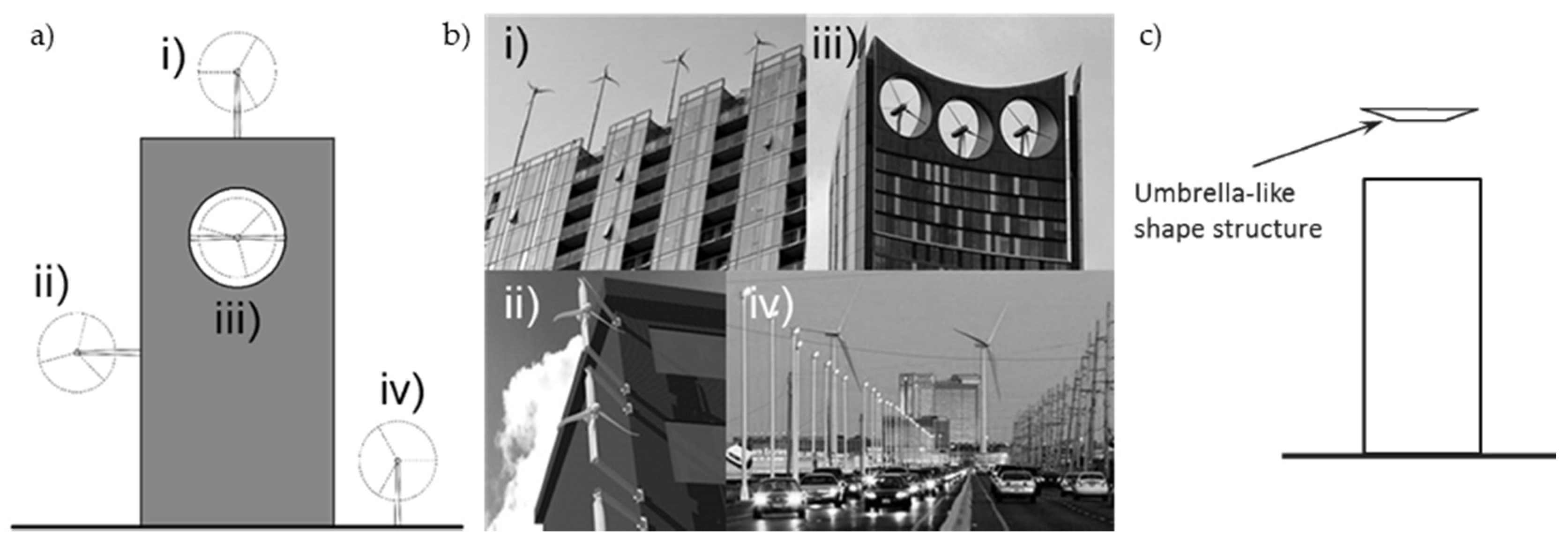
This work was funded under the European COST-Action TU1304 “WINERCOST” (Wind energy reconsideration to enhance the concept of smart cities), which considers each of the listed issues to improve knowledge on urban wind energy [10,11]. The positioning of wind turbines within the urban environment is one of the core issues. Performance of urban wind turbines is strictly related to the type of inflow they experience during their service life, and arguably a new type of wind turbine (WT) can be defined, i.e., the Building Augmented Wind Turbine (BAWT), or also Integrated (BIWT). Thus, the building is not only as a structural support to BAWTs, but also as an enhancer of the wind energy resource, as it diverts and concentrates the wind flow locally. Various types of WTs can be installed in many ways (Figure 1), depending on the mutual position between the building and the WT:
Another possibility is to enhance the flow by adding sub-structures to the roof of buildings to entrain and accelerate locally the wind, as shown in Figure 1c [17].
Investigations focusing on the assessment of the flow pattern aim at locating spots with optimal augmentation of the mean flow, with a limited assessment of the turbulence intensity to address areas to be avoided [2,18,19,20]. Studies generally agree in confirming that velocity augmentation and enhancement of turbulence intensity are the leading features of the flow pattern [21,22,23]. A rather limited amount of research has focused instead on the optimisation of the building shape to integrate BAWT with building architecture [13,14,24]. This has shown to be viable in a handful of applications, such as the Bahrain World Trade Centre [7]. Other works propose instead to enhance the energy yield by slightly improving the shape of the rooftop by building a collector directing the wind to the turbines to optimise the inflow [17]. Other studies also confirm that the shape of the roof is crucial in affecting parameters such as the extent of regions with higher turbulence intensity [19,23].
Most of literature on the wind energy resource above high-rise buildings uses Computational Fluid Dynamics (CFD) as a methodology to predict the wind speed [17,18,19,21,23]. However, the accuracy of CFD simulations should be verified and validated [7]. As field tests remain costly, wind tunnel tests are still viewed as the most reliable and effective technique to investigate the urban flows [7]. However, there are very few wind tunnel tests focusing specifically on wind velocity measurements. The most known experimental campaigns are the database published by the Architectural Institute of Japan (AIJ) [25] and CEDVAL database [26]. Both databases focus the attention to pedestrian level winds and not the flow over the building.
As mounting of WT on the top of the buildings represents the large majority of the applications (Figure 1i), an experimental campaign was launched to investigate the flow above the roof of high-rise buildings in the built environment using wind tunnel testing. Four wind directions α = 0°, 15°, 30° and 45° are considered in different geometric configurations: isolated high-rise building with two different roof shapes and in clusters of high-rise buildings. Measurements presented in this work are available publicly as Mendeley Data for the isolated building case [27] and clusters of high-rise buildings [28]. A previous work, based on the same experimental results, focused mainly on the flow pattern by predicting separation regions above the roof of the high-rise building. Based on the velocity and pressure fields flow pattern over the isolated building was analysed [29], while [30] focus on clustering effect. In addition, in [31] the flow above the flat roof was simulated using CFD approach. In contrast, the focus of the presented work is on the turbulence characteristics of the energy resource that a hypothetical wind turbine might face during its service life in various positions on the roof. Furthermore, it comprises all considered test cases with detailed comparison between them. The experimental setup is detailed in the next section. Turbulence statistics are then discussed for leeward and windward corners, edge locations and at the centre of the roof. At the end, the wind energy density of the wind resource is estimated based on the measured data.
2. Experimental Setup
2.1. Wind Tunnel Tests
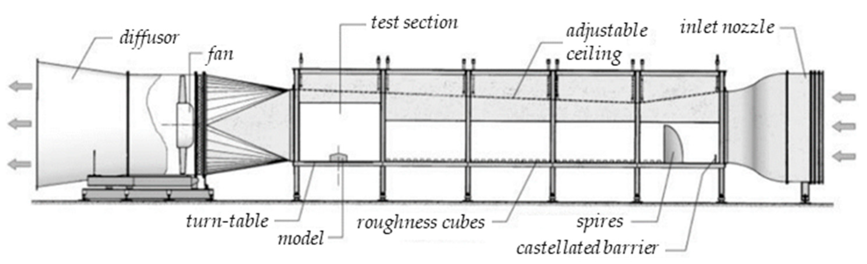
Wind tunnel tests have been conducted at the Atmospheric Boundary Layer (ABL) Wind Tunnel Lab of the Ruhr-Universität Bochum (RUB, Germany), with a cross section of and a length of , and an open tunnel configuration with the fan downstream of the test section.
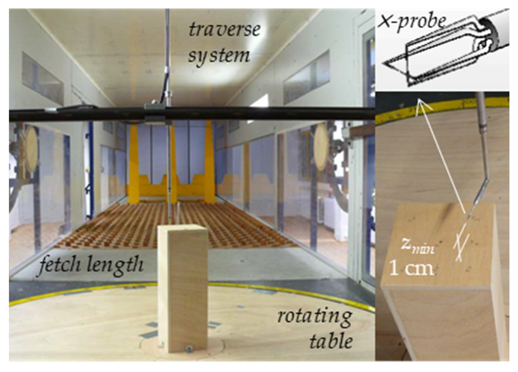
Figure 2 shows that the ABL is simulated thanks to turbulence generating spires and a castellated barrier, and roughness cubes (from 3.6 cm to 1.6 cm) capable of generating a broad variety of atmospheric boundary layer profiles. Measurements of the flow pattern were taken above the rooftop, using hot-wire anemometry (HWA). A miniature -wire probe of the DANTEC 55P61 kind has been placed at different heights above the model rooftop, using a traverse system. Figure 3 shows a configuration for the high-rise building model implemented in this study, with a detail of the HWA probe. The probe could not be positioned for distances smaller than due to the fact that HWA do not account for reverse flow.
To check the Reynolds number dependence, three different inflows velocity have been tested, with velocities around 9 m/s, 16 m/s and 18 m/s at the model height. Reynolds independence has been confirmed based on the measured pressure field. This is important as it was found that Strouhal number can be dependent on Reynolds number, in particular related to more stream-lined sections. In contrast, it is expected that this influence is rather small for bluff bodies, as separation positions are known [33].
Measurements have been taken to assure a good assessment of the turbulence intensity. The velocity components on the vertical plane u and w have been measured in the x and z directions, respectively, for z > zmin. Surface pressure measurements have also been performed using 64 pressure taps on the rooftop and on the sides of the building models. More details about the wind tunnel tests are reported in detail in [30] and are not further discussed in this work.
2.2. High-Rise Building Model
Two instrumented wooden high-rise building models have been used in this study. The building shape is that of a square prism with a height-to-width ratio of H/D = 3, where H = 0.4 m and D = 0.1333 m. The first model has a flat roof shape, while the second one a docked roof with an inclination of 30° superposed to the first model shape. The size of the model is compatible with a geometry scale of 1:300, or equivalent to a 120 m high-rise building, with sides of 40 m.
Four dummies replicating the shape of the flat roof building model have been also placed at a distance of 2D on the four sides of both models, to create the four configurations shown in Table 1. This is done to simulate isolated high-rise buildings and clusters of high-rise buildings. Four wind directions α = 0°, 15°, 30°, and 45° are finally tested to ensure a variety of ambient wind conditions.
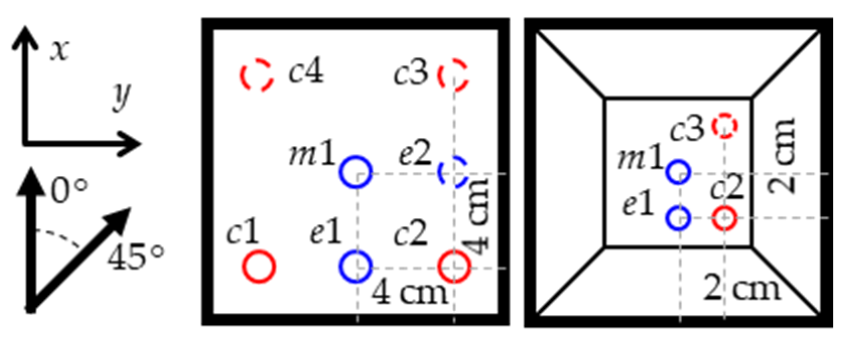
Figure 4 shows the position of the measurement locations above the roof in both docked and flat roof shapes. Locations have been chosen to investigate the wind energy resource at windward (c1 and c2) and leeward (c3 and c4) corner locations, windward (e1) and leeward (e2) edges and at the centre (m1) of the roof.
Due to the limited availability of the wind tunnel, the docked roof configurations have been measured for a reduced set of wind directions and positions. Configuration #3 has been measured only at positions e1 and m1 at α = 0° and 45°, while Configuration #4 has only been measured at at all positions shown on the right of Figure 4.
2.3. Velocity Profile
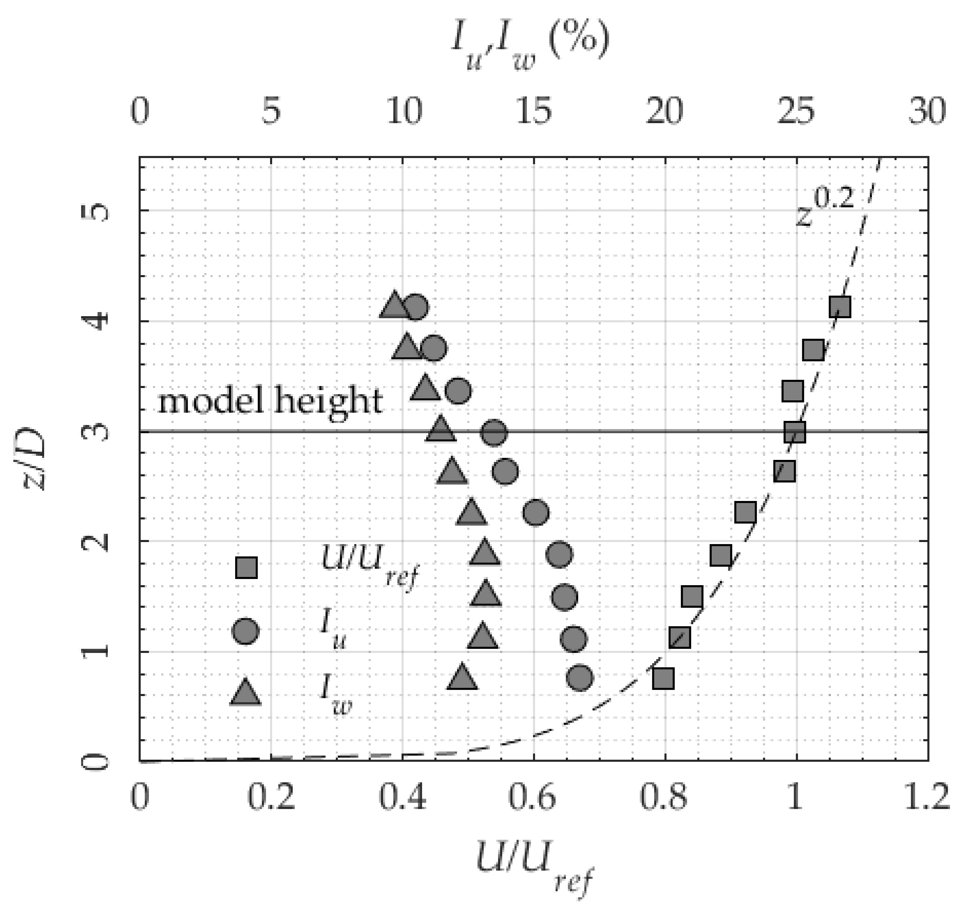
The atmospheric boundary layer wind speed generated in the wind tunnel best-fits a power law profile with an exponent of 0.2, as shown in Figure 5.
This is representative of a terrain category II, as defined in the Eurocodes [34], simulating realistic conditions of the flow around isolated high-rise building. Additionally, measured data can be used as an approximation for the flow pattern in case of an urban area with a dominant high-rise building surrounded by low-rise buildings. This arrangement is common on the outskirts of the large cities, university campuses displaced from city centres, etc. These all represent potential locations for efficient urban wind energy harvesting. The longitudinal turbulence intensity Iu at the building height is ~13%, with a vertical turbulence intensity Iw of ~11%. Iu and Iw below the height of the building grow steadily up to a value of 17% for Iu at 10 cm from the ground. The reference profiles are measured in the absence of the building model. Slight diverging trends seem to emerge for low values of z/D in Figure 5. This is associated with uncertainty level of the time-averaged stream-wise velocity that is in average around 5.6%, yet reaching higher levels close to the obstacles. Due to the manual positioning of the hot-wire anemometer, uncertainty related to the positioning of the probe is detected as one of the main uncertainty contributors. The curves presented in Figure 5 represent averaged values out of three measurement sets. More measurement sets would lead to smoother curve; however it would increase measurement costs. Thus, the number of measurement sets is kept at minimum while being able to extract the general trend of the curve. Measurement sets are also published as Mendeley Data [28] and more details on uncertainty estimation can be found in [30].
Results in the following are referred to the width of the model D and to the reference velocity as measured using a Prandtl tube placed at the wind tunnel walls, upstream of the model at the height of the building, (Figure 5).
3. Wind Energy Resource
The wind energy resource is presented in terms of mean wind speed, skew angle, turbulence intensity and integral length scale. Results are discussed based on the region above the roof. Windward corners are the roof regions where the flow is less disturbed by the coherent structures of the separated flow. Leeward corners experience severe turbulence and decrement of the wind speed due to the development of vortices. Windward and leeward edges are shown together with the centre position.
3.1. Flow Pattern
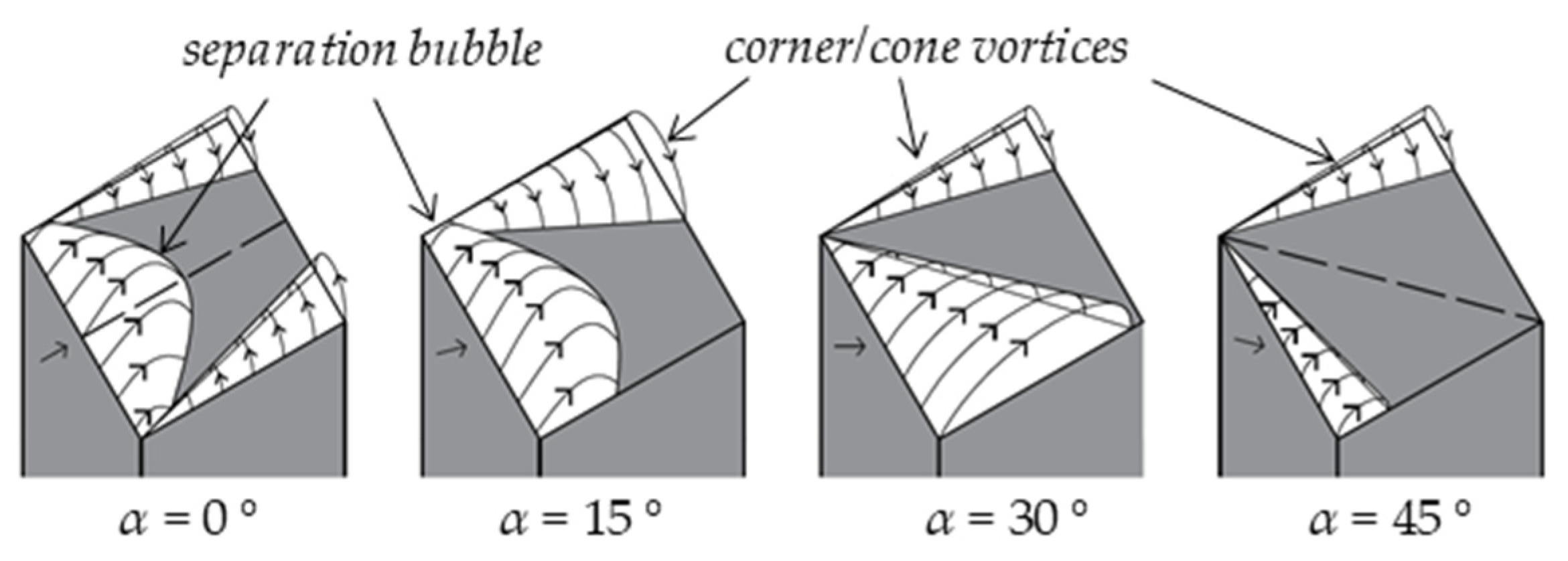
Previous numerical work has shown that a complex flow pattern takes place over the roof region of high-rise buildings [30,35,36]. The wind direction plays a fundamental role in affecting the coherent flow structures formation due to the separation taking place at the roof. In the case of flat roofs, at the windward edge, a separation bubble forms, which might reattaches creating a region of highly unsteady and intermittent flow close to the centre of the roof. Two cone vortices usually form at the edges parallel with the wind direction, which normally detach at the other end of the roof and merge with the shear layer from the separation bubble and the wake of the building. A similar flow pattern is also expectable for the docked roof shape. This flow pattern is known to take place on low-rise buildings from previous experimental evidence [37].
Figure 6 shows the expected flow pattern at various wind directions for the flat shaped roof, as reconstructed from the surface pressure as measured in this dataset (shown in detail in [29]).
Two of the configurations are symmetrical and the axis of symmetry is shown in the figure. If the flow direction is aligned to the edge of the square plant of the building, a separation bubble is present along with cone vortices. Otherwise, when the wind is aligned to the diagonal, only cone vortices are present.
3.2. Mean Wind Speed
The mean wind speed U is estimated taking the magnitude of the horizontal and vertical wind velocity components u and w. In this section, the wind speed is normalised with the freestream wind speed Uref measured at building height.
3.2.1. Windward and Leeward Corners
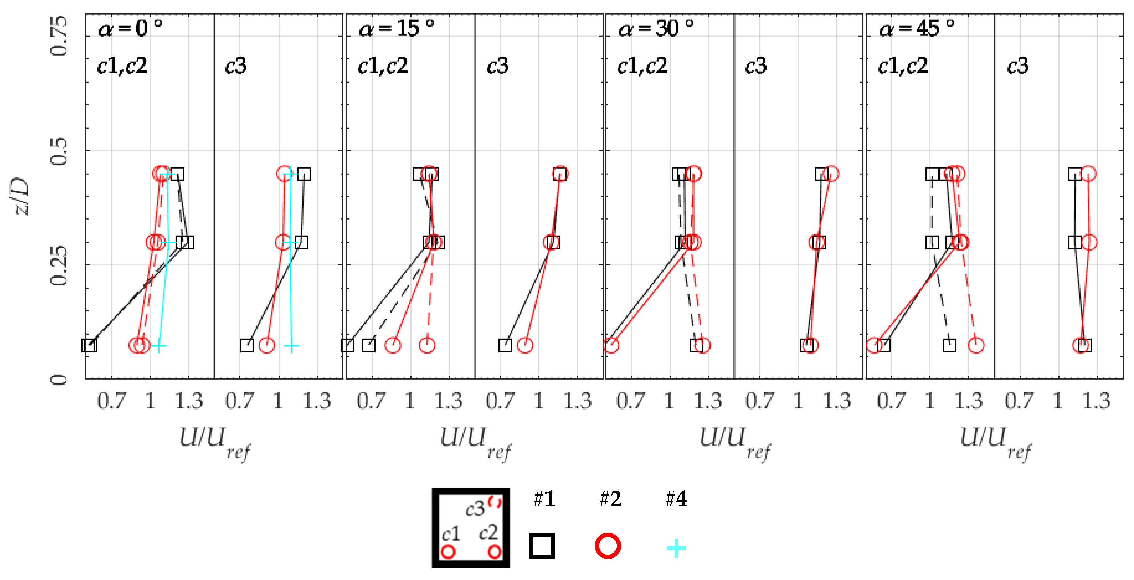
Figure 7 shows the normalised mean wind speed U/Uref as measured over positions c1, c2 and c3. Position c1 is dashed in the figure due to the symmetry of the wind direction. For α = 0° and , in isolated building configurations (configuration #1 from Table 1), the flow is likely to be separated close to the roof, analogously for the windward and leeward corners, with hot-wire anemometer returning lower wind speeds and high turbulence intensities >30% than those found at higher z/D. At the other wind directions closer to the roof, a marked difference between the two windward corners is noticeable, compatibly with the expected flow pattern for the different wind directions (Figure 6).
Buildings in clusters (configurations #2) do not differ significantly at and α = 45°, while the behaviour is markedly different for the other angles. This is compatible with the arrangement of dummy buildings, leaving a portion of undisturbed flow at those wind directions. Nevertheless, at , the disturbance of upstream buildings causes a reduction in wind speed at higher quotes from U/Uref ~1.3 of the isolated case to ~1 of clustering. However, the wind speed closer to the roof is improved in clusters for all affected wind directions, with a normalised wind speed of ~0.8 at α ≤ 15°, while for other wind directions an acceleration of ~1.3 takes place for shown configurations.
The docked roof shape was tested at locations c2 and c3 only for configuration #4 and α = 0° (Figure 7). In this case, the effect of the docked roof shows an increase in wind speed above windward and leeward points compared to configuration #2. Nevertheless, compared to the isolated building a reduction of wind speed above the roof and an increase close to the surface is the visible trend. However, depending on the wind direction this trend could be confirmed or denied.
3.2.2. Centre, Windward, and Leeward Edges
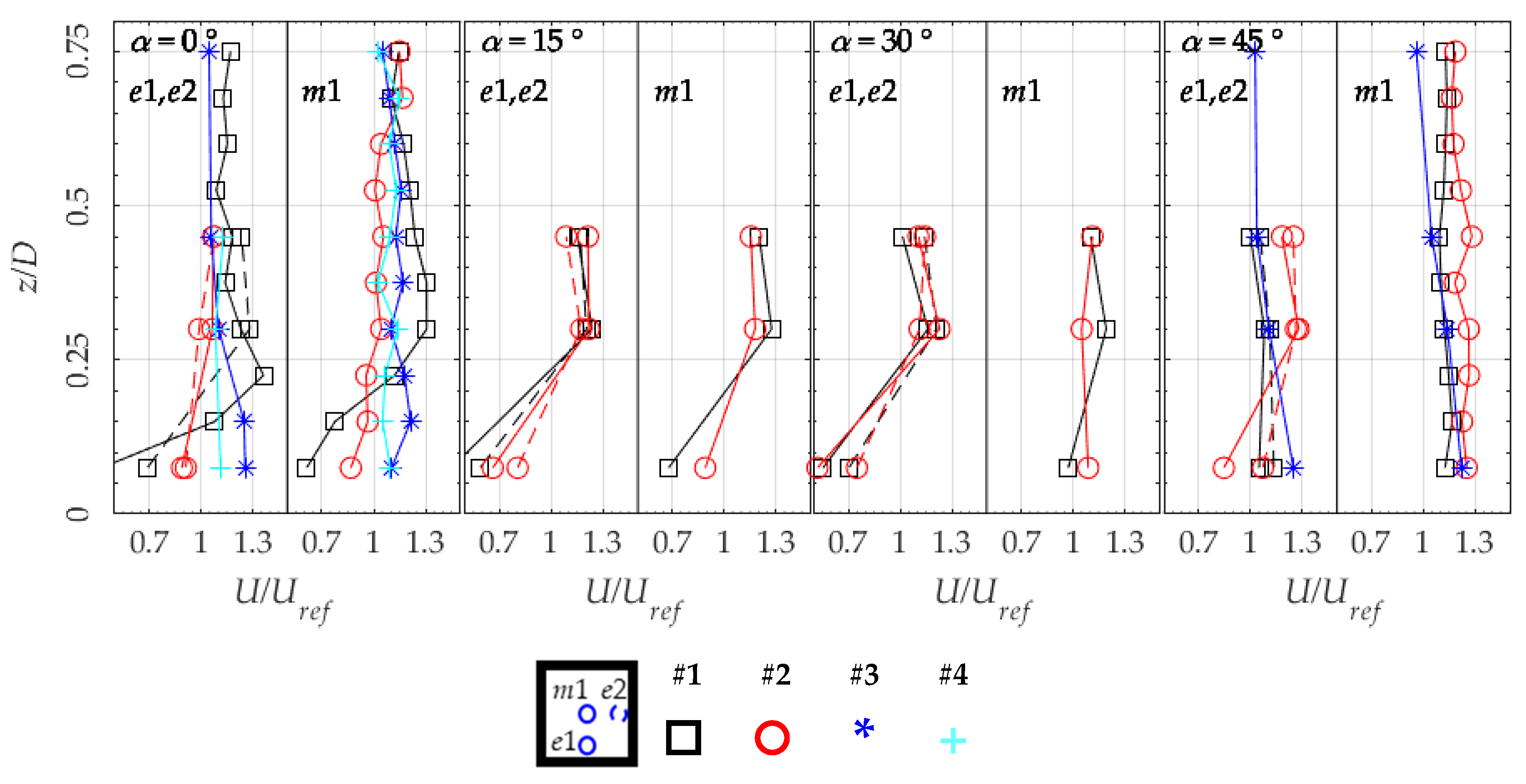
Figure 8 shows the normalised mean wind speed at the windward (e1) and leeward (e2) edges, as well as at the centre of the roof locations (m1). A region of separated flow is noticeable at z/D = 0.1 at position m1 for configuration #1, at 0° and 15°, which seems to disappear for other configurations and wind directions. The wind speed is rather uniform along the height where measurements were taken, with an enhanced value compared to the inflow wind profile. The highest increase in wind speed occurs in the configuration #1 at z/D~0.2 for 0°. At the centre of the roof the increased value occurs at z/D~0.3. The leeward edge e2 shows that having an obstacle upstream is beneficial to the wind speed, at lower heights. However, the effect is limited to α = 0°. The docked roof also is found to improve the uniformity of the flow. An increase in wind speed is present in all configurations at z/D > 0.3 and with the largest increase occurring for α = 0°. This could be explained by the presence of a large separation bubble, contraposed to cone vortices at other wind directions.
3.3. Skew Angle
One of the features of the flow pattern above the roof of high-rise buildings is the highly three-dimensional flow [38,39]. This may result in potential skewed angle of the wind speed, having a large impact on the performance of wind turbines. The skew angle is calculated using the longitudinal and vertical velocity components u and w.
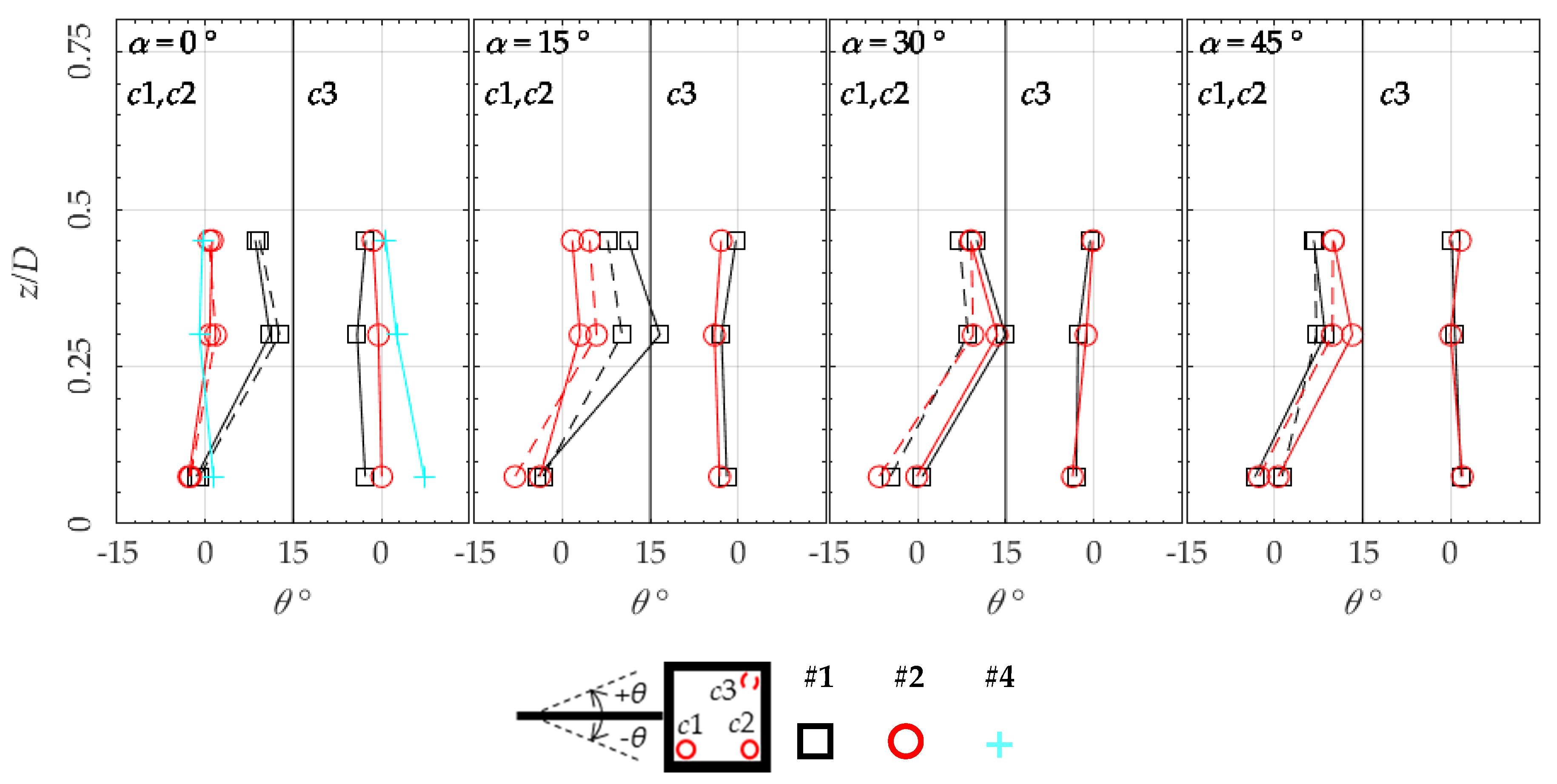
3.3.1. Windward and Leeward Corners
Figure 9 shows that both leeward and windward corners have a negative θ at z/D~0.1, while θ is positive at higher quotes. Clustering reduces the skew angle at α = 0° and 15°, with values consistently θ~0°. The isolated docked roof configuration, only tested at α = 0° and 45°, shows a nose-up skew angle at z/D~0.1, and θ~0° at higher quotes, showing the beneficial effect of shaping the roof in improving the flow pattern. The leeward corner is generally less skewed than the windward corner, which shows a nose-up θ for z/D > 0.1, consistently for all wind directions.
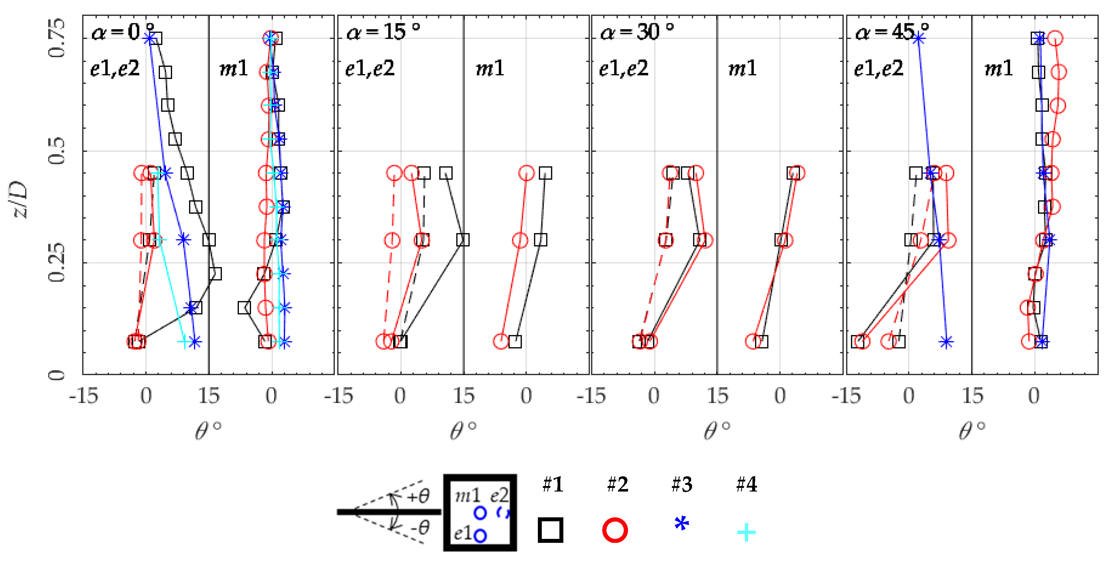
3.3.2. Centre, Windward, and Leeward Edges
Figure 10 shows the skew angle for the windward edge locations, showing the highest values in the dataset, with θ > 15° at z/D~0.2 and α = 0° for configuration #1. This is also the case for α = 15°, while for higher wind directions the skewed angle is reduced but steady around θ~12°. Clustering does not vary this trend for α ≥ 30° consistently with other locations. However, θ reduces at lower wind directions, showing the beneficial effect on flow around the border of the roof operated by the upstream flow. In configuration #3 and #4 the skew angle is reduced for z/D > 0.1. The flow is inclined to θ~10° at z/D~0.1 due to the inclination of the roof, which is also the case for configuration #3 and α = 45°. At the centre location m1, the skew angle is negative in the case of flat roof shape up to z/D~0.3 consistently for all wind directions, showing that the separated region is reattaching. Similarly to other locations, clustering reduces the nose-up flow, and θ is slightly negative for z/D > 0.3 at α = 0°, while it is weakly positive in other wind directions.
3.4. Turbulence Intensity
The longitudinal turbulence intensity is calculated using the mean wind speed . The vertical turbulence intensity shows an analogous behaviour to the longitudinal one, and therefore it is not shown in the following for the sake of brevity. However, the similarity of turbulence intensities gives some indications on the isotropy of the flow. In general, for z/D > 0.2, Iu~Iw, meaning that the turbulence is rather uniform and isotropic, close to grid turbulence and therefore easy to be reproduced in wind tunnels. This shows that it could be possible to use grid turbulence in wind tunnel testing for practitioners to design and test wind turbines in turbulent flows [40]. Such isotropic behaviour is not present at lower heights (z/D < 0.2), where the longitudinal component is significantly higher than the vertical one. This anisotropy indeed has an effect on the behaviour and aerodynamic response of devices placed in its stream and at present there is no convincing technique to reproduce this rate of anisotropy in the wind tunnel without a significant and expensive amount of trial and error, so unfeasible for practitioners investigating the response of wind turbines. However, in those areas the highly skewed and disturbed flow conditions are not usually relevant to the positioning of wind turbines.
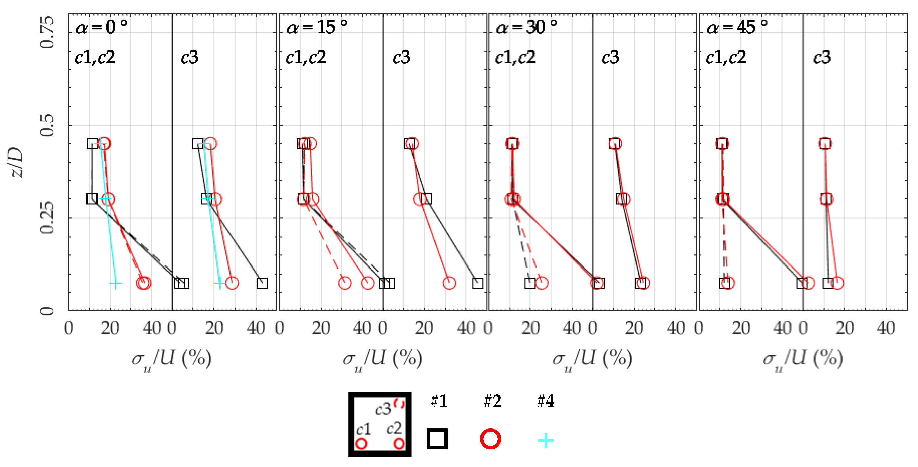
3.4.1. Windward and Leeward Corners
Figure 11 shows corner locations c1, c2, and c3. The atmospheric wind profile at building height is Iref~12% and generally this is the turbulence intensity noticeable above the roof for z/D > 0.3 for the isolated high-rise building configuration. Figure 11 shows that the building seems to affect turbulence intensity up to a height of about one third of its width. At z/D~0.1, the turbulence intensity is the highest , and this is incompatible with the serviceability of wind turbines, as the IEC allows a maximum Iu = 15% [41]. However, z = 3 m is a common installation height for small wind turbines on buildings. A height of z/D~0.3 corresponds to turbulence intensities of the order of Iu~12%, meaning that ideally at least a 10–12 m mast over the rooftop of high-rise buildings would be necessary to comply to values indicated by IEC standards for the reference turbulence intensity or for a wind turbine to avoid the region with high turbulence [41,42].
Clustering reduces Iu at corners if α = 0° and 15°, while it slightly increases it at α = 30° and . The windward corner c1 shows a turbulence intensity comparable to Iref, expectably due to the favourable position of the windward corner. The clustered docked roof configuration shows a lower Iu at α = 0°, confirming the beneficial effect of modifying the roof shape on the wind resource.
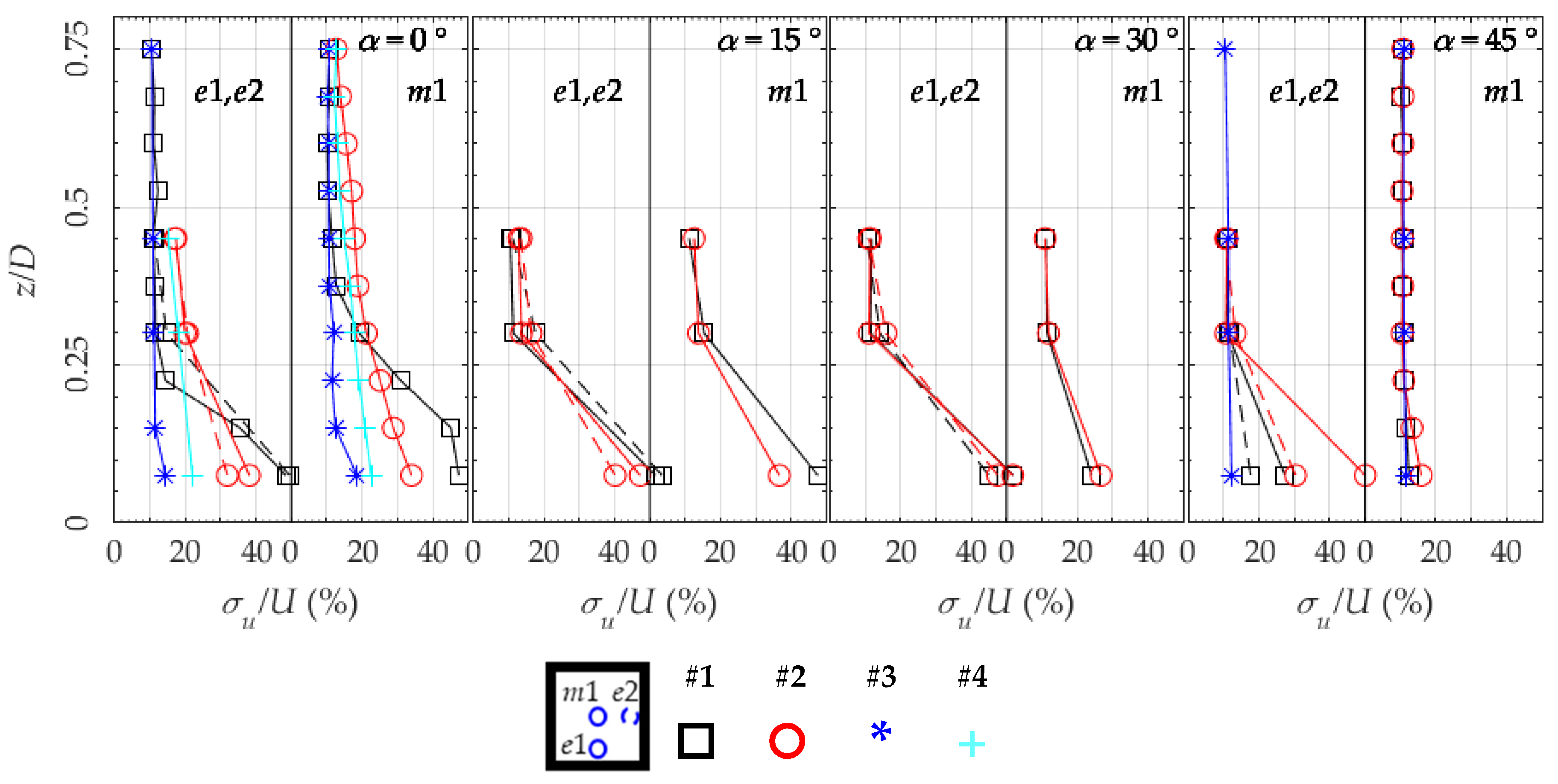
3.4.2. Centre, Windward, and Leeward Edges
Figure 12 shows the edges and centre locations. The denser measurements points confirm that the disturbed flow region extends to z/D~0.3 at α = 0°. Configuration #1 shows the highest turbulence intensity of the dataset at all positions. Clustering seems to increase the expected turbulence intensity even at z/D > 0.3 for both roof shapes for α = 0°, while the docked roof shape is found to greatly reduce the turbulence intensity at z/D < 0.3 for α = 0° and 45°. This could be interpreted with the larger disturbed region of the flow around the cluster, engulfing the roof area of the building.
3.5. Integral Length Scale
The integral length scale of turbulence is calculated applying the Taylor hypothesis and using the autocorrelation coefficient , where is the autocorrelation function, and is the time lag. The integral yields the integral time scale and , where is the mean velocity [43]. In this work, the integral is calculated considering the first 0 crossing of , i.e., , where, and is estimated using a simplified relation where [44]. The reference integral length scale calculated using the atmospheric wind profile at building height yields .
3.5.1. Windward and Leeward Corners
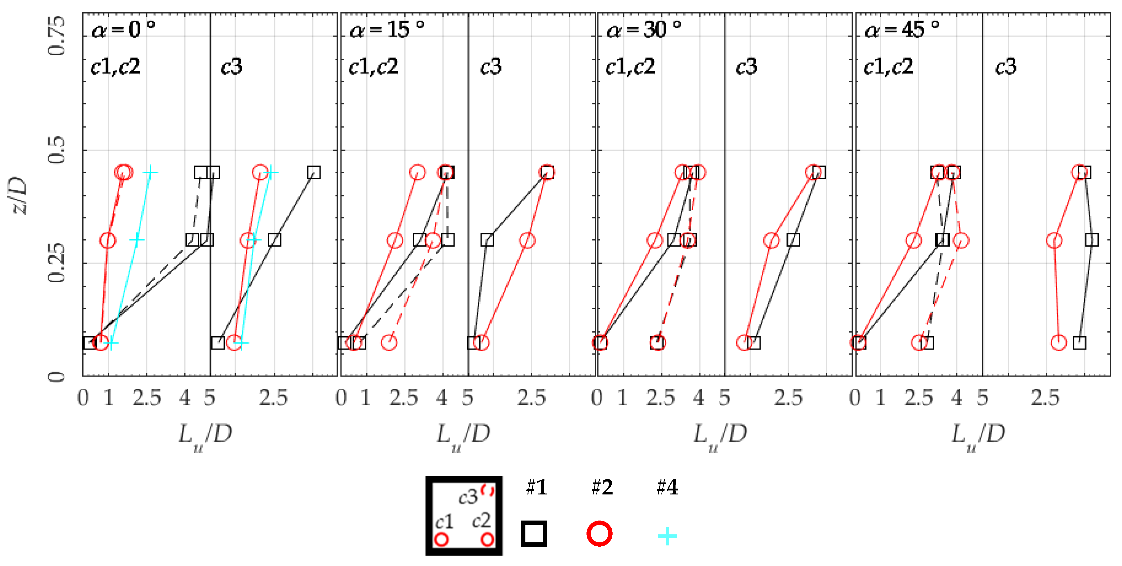
Figure 13 shows for the corner locations. In addition, analogously to what is found for the turbulence intensity, most data converge to at z/D~0.3. Lu shows a monotonic growth with height for the windward and leeward corners. Clustering reduces the size of the length scale by a factor of ~3 at α = 0° at z/D > 0.3. A slight reduction is also noticeable for the docked roof shape, and in that case clustering follows the same pattern as observed for the flat roof. As for configuration #1, length scales at z/D~0.3 and 0.45 converge towards similar values to Lref at the leeward corner, while the windward corner shows a monotonic growth with height. The growth rate is greatly reduced in configuration #2, and in general clustering reduces the size of vortices, possibly due to the fact that the model is enclosed in the wake of upstream buildings.
3.5.2. Centre, Windward, and Leeward Edges
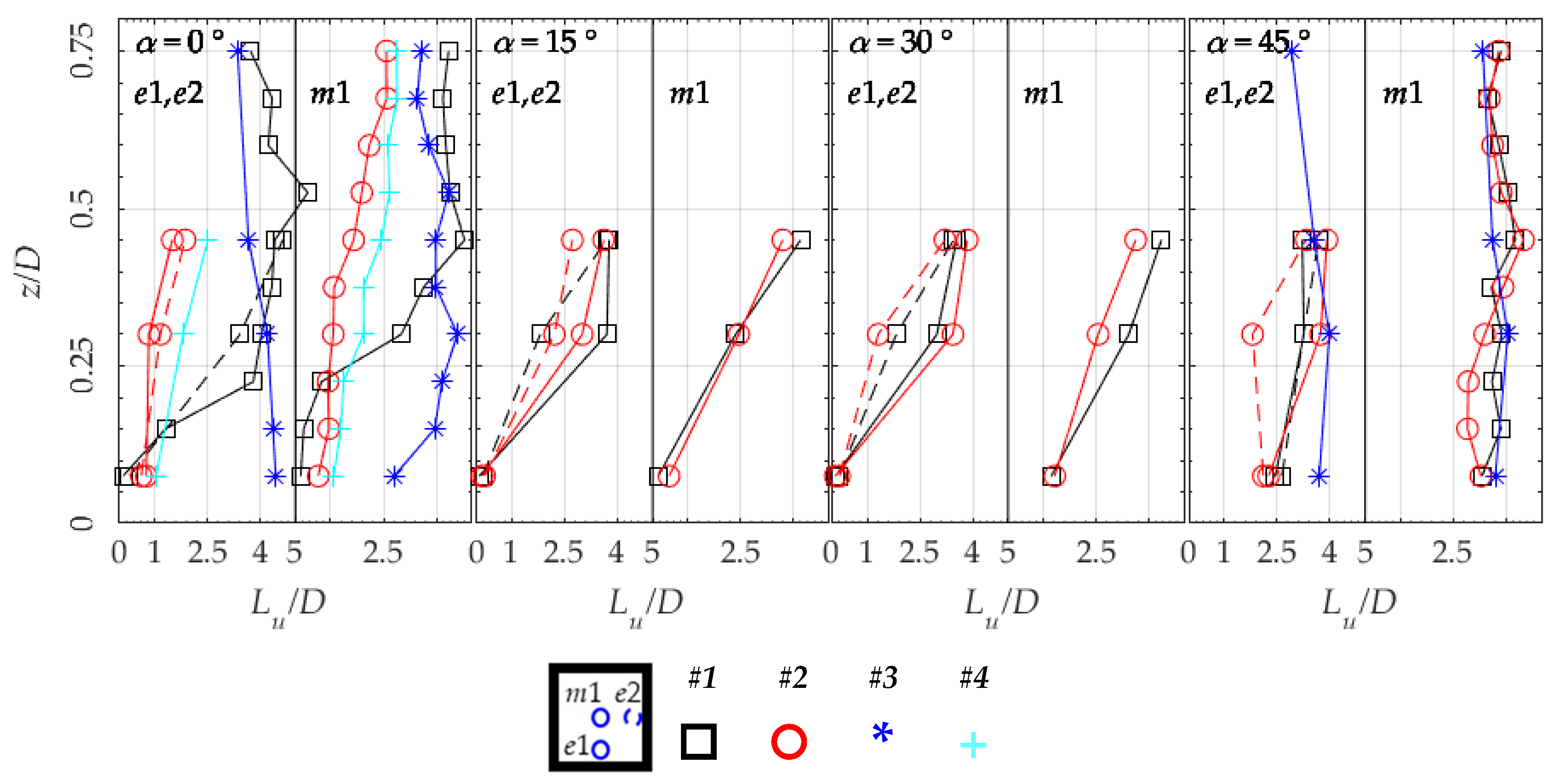
Figure 14 shows the edge and centre locations. For configuration #1, the length scale gradually increases towards Lref up to z/D~0.2, to then maintain that value at other heights for all wind directions. Configuration #2 shows a different behaviour to #1 at α = 0°, with a sensibly smaller length scale (comparable to Lref/2 instead of Lref, which might indicate a larger extent of the separated flow region [32]). For the centre location of configuration #1, the behaviour is different between α = 0° and the other directions. For α = 0°, Lu increases steadily towards Lref up to z/D~0.3–0.4, while for the other wind directions Lu increases in a similar manner for both configurations #1 and #2. At α = 45° the length scale shows similar values at both lower and higher quotes, showing the effect of the cone vortices and the relatively undisturbed flow region at the centre of the roof. The docked roof configurations #3 and #4 show a reduction of the length scale similar to configuration #2 at α = 0°, and larger uniform values at α = 45° for configuration #3.
Results on the integral length scale show that wind turbines placed at z/D > 0.3 experience a flow with coherent structures similar to those found in freestream atmospheric conditions, i.e., a length scale with a size comparable to the building rather than the wind turbine blade or rotor diameter. At lower heights, where small wind turbines are likely to be installed, the length scale is reduced dramatically, with unclear repercussions on the aerodynamic performance and power output. In fact, at z/D~0.1, the integral length scale is equivalent to ~5–10 m, hence it is comparable to the size of rotors.
3.6. Energy Spectra
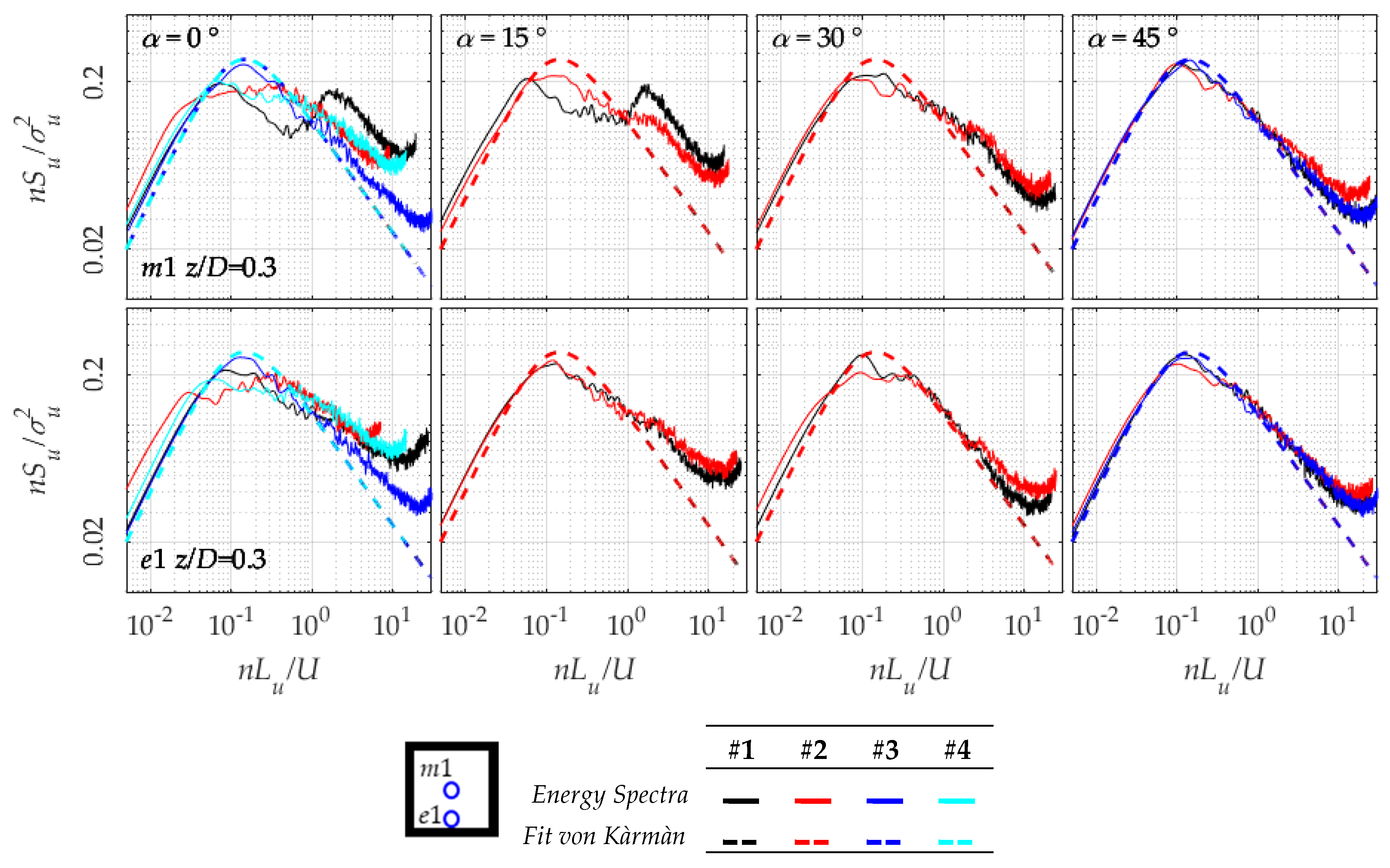
To further compare the behaviour of the roof flow region with the atmospheric wind, Figure 15 shows the power spectral densities for the windward edge e1 and centre m1 locations (respectively, upper and lower rows) at z/D = 0.3 or z = 12 m for the various configurations and wind directions as indicated. The von Karman Spectrum, as calculated using the integral length scale Lu, is also computed and plotted together with the results. U is the mean wind speed, n is the frequency in Hz and the wind speed variance. Results are consistent with findings of Figure 13 and Figure 14, with the different configurations diverging from the von Karman spectrum at α = 0° (Figure 15).
The configuration with the closest resemblance to the atmospheric wind is configuration #3, where no high frequency peaks are noticeable from the energy spectra. However, a slight peak is noticeable at nLu/U~2. Similar high frequency peaks can be observed for the other configurations for α = 0° and 15°, with configuration #1 experiencing the most evident peak. This is compatible with a measurement point taken in the shear layer where a vortex sheet is forming. Energy spectra aid in the detection of the shedding of vortices, which is important to assess due to possible resonance effects on wind turbine masts or other components installed above the roof [24]. In this study, configuration #1 is prone to vortex shedding at the centre location, while the effect is milder.
Clearly in clustering, this is disrupted by the presence of surrounding buildings or the different shape for the roof, although some periodicity at those frequencies is still present.
4. Probability Distribution Function
One of the most significant outcomes from an environmental study on the wind energy resource is the assessment of the probability distribution function (PDF). By fitting the distribution, it is possible to obtain general expressions to aid with the modelling of a realistic wind resource. The present dataset has been normalised against the standard deviation and its PDF fitted to a Weibull distribution for each time-history of the dataset:
Some of the measurements have been repeated to check the quality of the time-histories (in accordance with checks on the extension of the separation bubble), and no variation of the freestream velocity has been operated. The Weibull distribution of the freestream velocity of building height has a shape factor k = 8.6. Above the roof, it has been found that the shape of the Weibull distribution is consistent for all configurations and wind directions, with the scale parameter yielding a~5.6–6.2 and the shape parameter analogous to the freestream k~6–8. The shape parameter for ambient wind taken over an extensive period of time resembles a Rayleigh distribution, i.e., k~2. This study has the limitation of the sample period only considering a limited amount of information. Nevertheless, it is significant that the PDF for different configurations and wind directions takes a similar shape if z/D≥0.3 or z ≥ 12 m, as this can be considered a safe distance from the building where turbulence intensity is analogous to ambient turbulence.
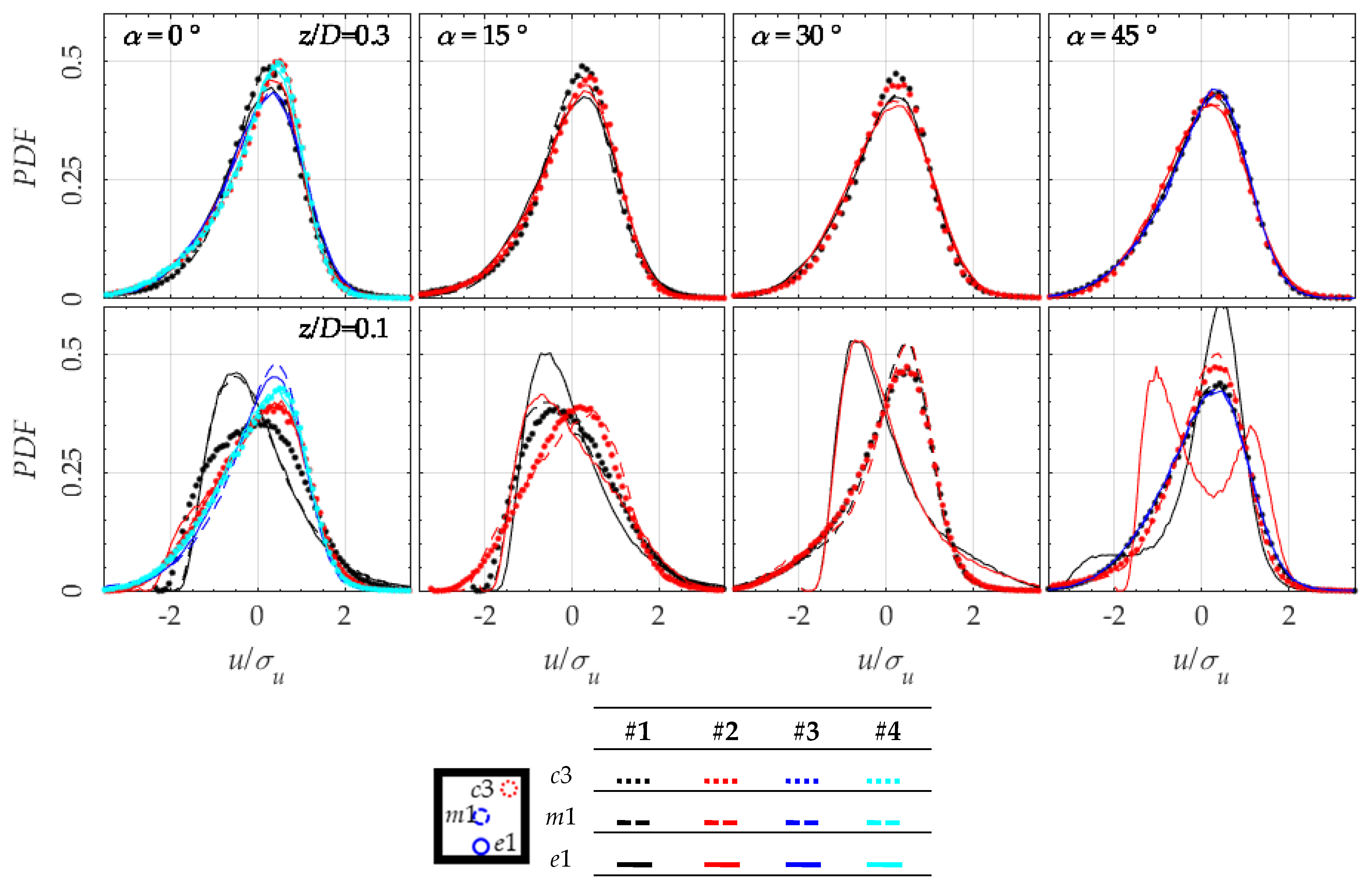
Figure 16 shows the PDFs taken at z/D = 0.1 and z/D = 0.3 for three locations, i.e., windward edge, centre and leeward corner. The shape of the PDF at the lower quote (lower row) shows negative fat tails and is positively skewed for the corner and centre locations. For the edge location the shape of the PDF varies with the wind direction, with a bimodal distribution noticeable at α = 45° for configuration #2, possibly due to vortex shedding interacting with the local flow and causing an intermittent wind speed. While the same trend can be observed for α = 0°, for higher wind directions the distribution is negatively skewed with positive fat tails. This is consistent for both configurations #1 and #2. For α = 30°, the PDF normalises for configuration #2.
At α = 45° the PDF is analogous to higher quotes, with the exception of configuration #1 which show still a negative skewness with positive fat tails. At z/D = 0.3 the distribution is analogous at all configurations and locations, with positive skewness and negative fat tails. In all cases and quotes the docked roof configurations show an analogous wind distribution, normalising the behaviour.
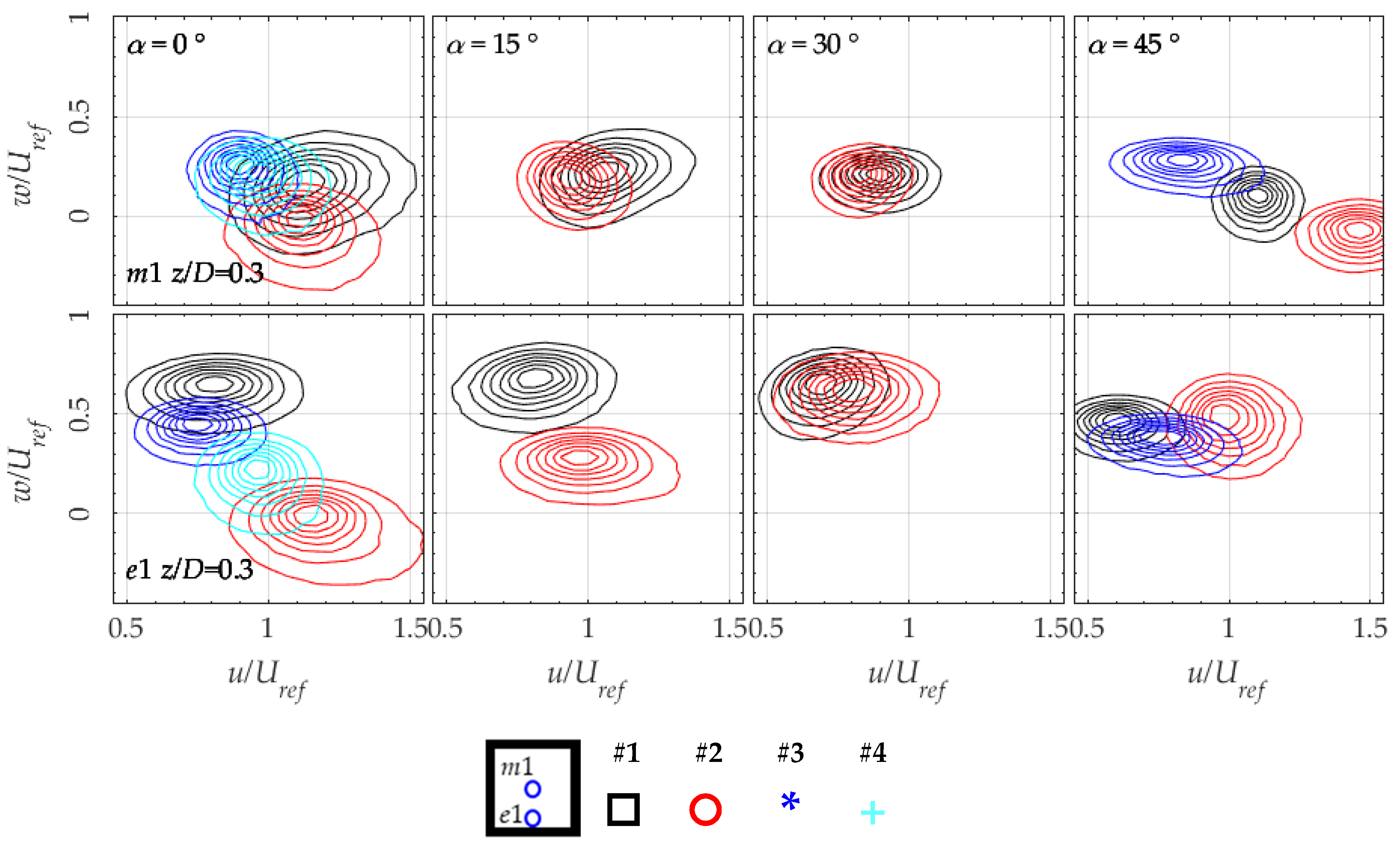
Quadrant Analysis
The joint probability distribution function (JPDF) can be useful to understand the physics of a turbulent flow in terms of dominance of a wind component with respect to the other. Figure 17 shows the JPDF for locations e1 and m1 at z/D = 0.3. For α = 0°, the mean wind speeds of all configurations are comparable to Uref for building clusters, and they slightly differ for the isolated building at both positions. The main difference is the vertical component, which is ~0 for configuration #2 and ~0.75 for configuration #1 showing the large variability of skewed angle. The horizontal spread of the contour plot signifies a lack of variability of the vertical wind component, and it is significant that configuration #4 shows the largest variability of w. In the centre position m1, all contours insist on the origin of the plot at α < 45°, meaning that a similar mean wind speed is present in different configurations. However, the variability of w is enhanced, showing the unsteady behaviour of the shear layer above the reattachment region of the roof.
In general, the trend of a larger variability of the vertical component w can be observed for all wind directions and configurations, with a more limited variability for clusters.
5. Wind Energy Density
In order to understand the expected performance of a model wind turbine operating on a high-rise building, an evaluation is proposed of the available wind energy density, giving some indications on the turbulence intensity on the various roof locations.
The wind energy density of the wind resource is calculated for a unitary area considering the mean wind speed on a specific location.
The following figures interpolate across the locations of the dataset to obtain a wind energy density map and locate positions where the maximum and minimum yields are to be expected for the different wind directions. To improve the density of points, for symmetric wind directions α = 0° and 45°, positions e2 and c2 are mirrored with respect to the symmetry axis. The missing points at other wind directions are instead interpolated from the closest positions using a cubic interpolation algorithm. No point in the dataset is extrapolated and due to the coarseness of measurements points the docked configurations #3 and #4 are omitted in the this section. However, relevant conclusions can be made also from the wind speed plots of Figure 7 and Figure 8.
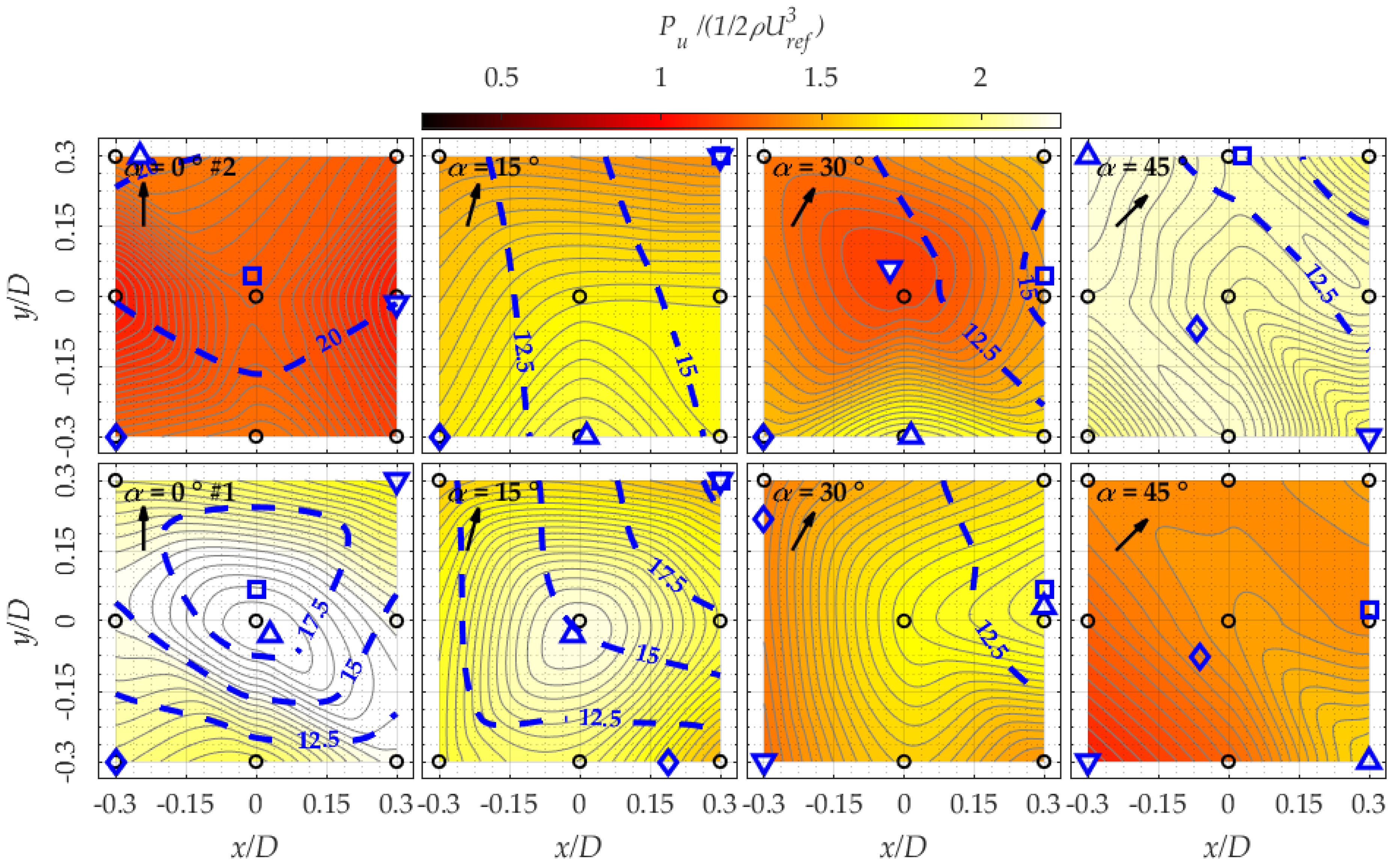
Figure 18 shows Pu at z/D = 0.1. This height corresponds to common locations where a small wind turbine might be installed in the built environment. Pu is normalised against the wind power as calculated using Uref, or the power which would be available in the absence of the building. Configuration #2 (top row) shows that in general a cluster of buildings benefits the energy available at lower height compared to the isolated building configuration. The windward corner is the region where most power is to be harvested, with an increment of harvestable energy up to ~+50% at α = 45°.
Figure 18 also shows contour lines for the turbulence intensity at z/D = 0.1. All over the roof the turbulence intensity has values around 30%. The worst wind directions are those which cause a separation bubble to occur, i.e., α = 0° and 15°. At α = 45°, the corners at the transversal diagonal of the building perimeter yield the lowest energy, with a decrease in power of , while on the other diagonal an increment of >100% occurs. This is telling towards positioning strategies. If high values for the turbulence intensity are somehow accepted, a good approach to implement urban wind energy at low heights can be the installation of multiple small devices at all corners of the roof. In this way, devices in suitable locations make up for the reduced power of other locations. In fact, at this height, the best values are measured at corners in all wind directions. The worst performing locations are the edges of the building, which should be avoided due to both the low energy and the high turbulence. The centre of the roof has instead a good yield, on the same order of magnitude of the undisturbed power. When the building is isolated in configuration #1, the energy yield is in general not favourable as if the wind direction is α = 0° or 15°, or if a separation bubble is present. Cone vortices are found to be less turbulent and for α = 30° and 45° an energy gain is noticeable, with the isolated model and the clustered one behaving similarly.
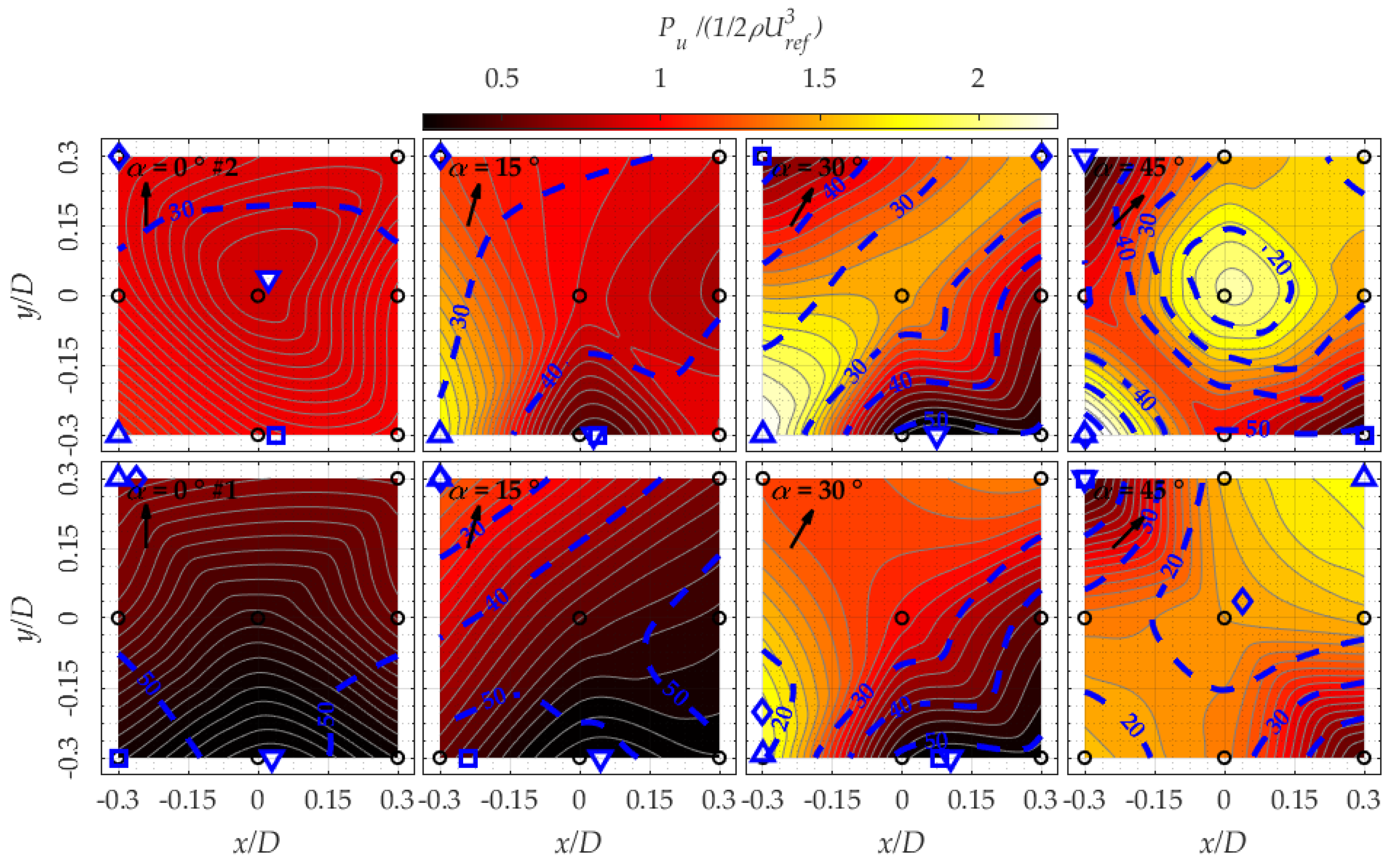
Figure 19 shows the wind energy density at z/D = 0.3. Unlike z/D = 0.1, clustering strongly reduces the energy yield and increases the turbulence intensity at α ≤ 30°. The isolated building configuration is particularly beneficial to the wind resource with increments of the available power up to 2.6–2.8 times for α = 0° and 15°. In fact, configuration #1 shows that the centre location is the most productive of the dataset, with corners strongly underperforming. Vice versa, configuration #2 sees the beneficial effect of the accelerated flow, with power of the order of magnitude of the undisturbed flow for α ≤ 30°. In this case it is trickier to evaluate the best position, with corner locations possibly preferred due to the lower turbulence and slightly higher acceleration of the flow shown in Figure 19. Clustering also increases the turbulence intensity, especially at α = 0°.
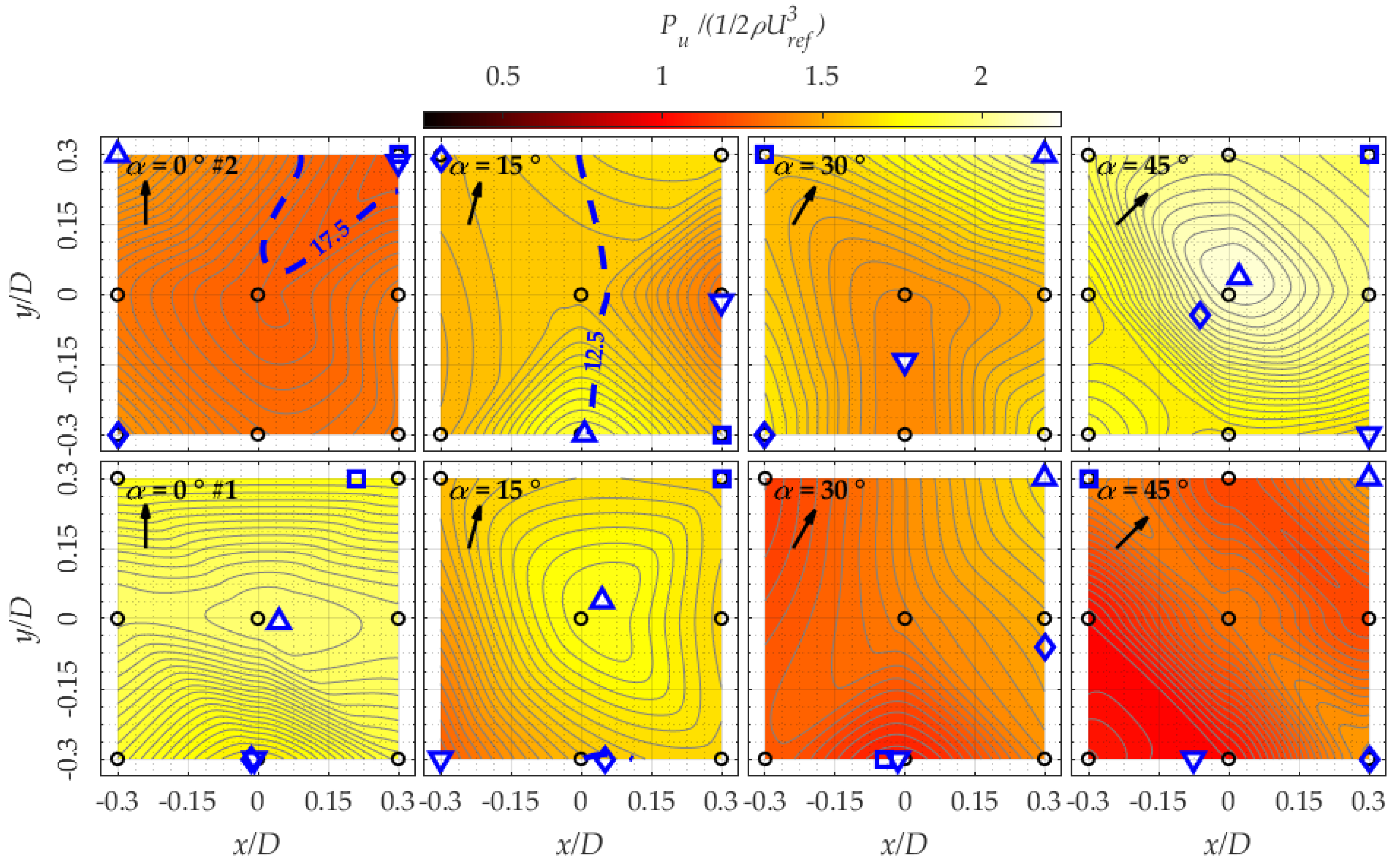
Figure 20 shows results for z/D = 0.45 or z = 18 m, which might be constructively complex to realise on existing buildings, but it might be relevant to the size of small wind turbines (~10 m in diameter for a HAWT). Similar conclusions to Figure 19 can be drawn, with a lower power from configuration #2 and a slight increase for configuration #1 reaching up to 1.5–1.8 increase in power. The centre location looks in this case to be the most suitable location, although in several wind directions the corner is the most and also the worst performing location. At this height, the turbulence intensity is rather uniform with values Iu~10–12% analogous to the atmospheric turbulence.
In terms of incrementing the wind energy resource, it can be argued that cluster of high-rise buildings are only beneficial at α = 45°, where a channelling effect takes place among the dummies and the central building.
With wind energy density maps, as those shown in Figure 18, Figure 19 and Figure 20, a positioning strategy for wind turbines can be developed. The energy resource over the whole of the roof region is to be analysed to estimate the yield of an urban wind turbine.
In particular, the distribution of multiple devices might be a promising strategy to tackle the very different behaviour for varying wind directions, as also suggested in previous research [19]. The optimal height to install devices for this dataset is z~12 m, while installing with turbines on edges should be avoided, as the roof flow shows the least potential in such areas. If turbulence intensity is less concerning (fixed direction, ducted or vertical axis devices), corner locations at z~3 m can be exploited as they experience an acceleration, as well as the centre region. At z = 12 m the turbulence intensity is much reduced, with a reduced wind shear analogous to atmospheric values. This allows for larger devices to be placed in optimal flow conditions at the centre of the roof, provided that structural safety is guaranteed.
A question arises, whether turbulence should be avoided, a rather difficult limitation to respect, or exploited, and much research is needed to understand how turbulence affects the behaviour of aerodynamic devices [32].
6. Conclusions
In this study, the flow above the roof of a high-rise building is investigated under various wind directions to assess the wind energy resource at several locations. The flow can be divided into three distinct regions:
- A region close to the roof surface z/D = 0.1 where turbulence is exclusively affected by the building itself. In this region, the wind speed is relatively low in magnitude and dominated by separated flow, while the turbulence intensity is at its highest (>20–30%). The integral length scale is also smaller than the characteristic size of the high-rise building, with increased isotropy. In this region, the experimental results from hotwire anemometry might be misleading due to the insensitiveness to reversed flow conditions which characterises the flow field. Weibull parameters in this region diverge from those found in the atmospheric wind profile.
- A region of highly sheared flow at z/D~0.3–0.4. The position and extent of this region varies with the wind direction and configuration of the building. The velocity is weakly accelerated and combined with relatively low turbulence intensity Iu~15%. The Weibull distribution is analogous to the atmospheric flow with a shape factor k~8–9.
- A region of accelerated flow, which is highly influenced by the atmospheric wind profile at z/D~0.45. Both mean wind speed and turbulence are analogous to the inflow, U~Uref and Iu~12%, having integral and microscales comparable to atmospheric boundary layer values.
Wind turbines are normally placed quite close to the roof surface, so as to avoid expensive substructures not (yet) justifiable from the perspective of the energy efficiency of the wind turbines installed. The present study suggests that an effective design of small wind turbines installed on buildings will necessarily take into consideration yawed and intermittent inflow characteristics. Table 2 summarises the findings for the wind directions.
The square plan high-rise building is strongly affected by the wind direction. The docked roof shape improves the behaviour as the flow at the measured locations shown in this study is quite insensitive to the variability of the wind. However. More locations are to be investigated to draw further conclusions. Nevertheless improving the shape of the roof by tilting it seems to be a feasible way of enhancing the wind energy resource.
The region z/D < 0.3 is characterised by reversed flow associated with high turbulence and a smaller velocity magnitude. It is advisable to avoid this region altogether to have a significant gain from wind energy harvesting. However, the corner locations of the roof might be less affected and, in fact, show acceleration of the flow and stretching of turbulence, which might be beneficial to the performance of multiple wind turbines compensating for each other’s lack of performance based on wind directionality.
The region z/D > 0.3 shows an increase in the available atmospheric power, due to the flow avoiding the obstacle posed by the high-rise building, at all configurations and wind directions, with a turbulence intensity comparable to the atmospheric one. However, significant complications might arise due to the installation of large rotating machines on masts up to 10–15 m, if a careful structural assessment is not done prior to the construction. Therefore, it is essential that an assessment of the wind resource has to be made with simulation tools, such as wind tunnel testing or computational fluid dynamics, to estimate the potential yield of devices.
The local Weibull distribution could be useful to predict the Annual Energy Output of a roof farm, by adapting the freestream wind to local flow features. This study suggests that at z/D > 0.3 a shape factor analogous to the one found for the freestream wind can be used. However, at lower heights, the shape factor varies from k = 2 to k = 6–8, depending on the local turbulence and wind speed. It is therefore advisable to carefully consider the wind direction and actual probability distribution to plan the installation of wind turbines close to the surface of the roof.
More research is needed to characterise the above-roof region with dependence on the surroundings and the shape of the building itself using techniques capable of predicting turbulence rather than mean velocity. These preliminary results show the need for a high-fidelity approach for the modelling of the turbulence pattern around building for wind energy harvesting.
Author Contributions
Conceptualization, G.V. and S.S.; methodology, G.V., A.Š.-G. and H.H.; formal analysis, G.V.; investigation, A.Š.-G. and H.H.; resources, C.B.; writing—original draft preparation, G.V.; writing—review and editing, G.V., A.Š.-G. and S.S.; supervision, S.S. and H.H.; project administration, C.B.; funding acquisition, C.B. All authors have read and agreed to the published version of the manuscript.
Funding
This research was funded by the COST Action TU1804 WINERCOST—“Wind Energy to enhance the concept of Smart cities” through a Short Term Scientific Mission to conduct the experiments. The support of the European Commission’s Framework Program “Horizon 2020” through the Marie Skłodowska-Curie Innovative Training Networks (ITN) “AEOLUS4FUTURE—Efficient harvesting of the wind energy” (H2020-MSCA-ITN-2014: Grant agreement no. 643167) is also acknowledged. Also, this work was supported by the Luxembourg National Research Fund (FNR) under project reference C19/SR/13639741.
Conflicts of Interest
The authors declare no conflict of interest. The funders had no role in the design of the study; in the collection, analyses, or interpretation of data; in the writing of the manuscript, or in the decision to publish the results.
References
- Stathopoulos, T.; Alrawashdeh, H. Urban Wind Energy: A Wind Engineering and Wind Energy Cross-Roads; Springer: Cham, Switzerland, 2019; pp. 3–16. [Google Scholar]
- Micallef, D.; van Bussel, G. A Review of Urban Wind Energy Research: Aerodynamics and Other Challenges. Energies 2018, 11, 2204. [Google Scholar] [CrossRef] [Green Version]
- Fuglsang, P.; Bak, C.; Schepers, J.G.; Bulder, B.H.; Cockerill, T.; Claiden, P.; Olesen, A.; van Rossen, R. Site-specific Design Optimization of Wind Turbines. Wind Energy 2002, 5, 261–279. [Google Scholar] [CrossRef]
- Bontempo, R.; Manna, M. The axial momentum theory as applied to wind turbines: Some exact solutions of the flow through a rotor with radially variable load. Energy Convers. Manag. 2017, 143, 33–48. [Google Scholar] [CrossRef]
- Moeini, R.; Tricoli, P.; Hemida, H.; Baniotopoulos, C. Increasing the reliability of wind turbines using condition monitoring of semiconductor devices: A review. IET Renew. Power Gener 2018, 12, 182–189. [Google Scholar] [CrossRef]
- Martin, C.M.S.; Lundquist, J.K.; Clifton, A.; Poulos, G.S.; Schreck, S.J. Wind turbine power production and annual energy production depend on atmospheric stability and turbulence. Wind Energ. Sci. 2016, 1, 221–236. [Google Scholar] [CrossRef] [Green Version]
- Stathopoulos, T.; Alrawashdeh, H.; Al-Quraan, A.; Blocken, B.; Dilimulati, A.; Paraschivoiue, M.; Pilay, P. Urban wind energy: Some views on potential and challenges. J. Wind Eng. Ind. Aerodyn. 2018, 179, 146–157. [Google Scholar] [CrossRef]
- Hansen, K.S.; Barthelmie, R.J.; Jensen, L.E.; Sommer, A. The impact of turbulence intensity and atmospheric stability on power deficits due to wind turbine wakes at Horns Rev wind farm. Wind Energy 2012, 15, 183–196. [Google Scholar] [CrossRef] [Green Version]
- Pagnini, L.C.; Burlando, M.; Repetto, M.P. Experimental power curve of small-size wind turbines in turbulent urban environment. Appl. Energy 2015, 154, 112–121. [Google Scholar] [CrossRef]
- Baniotopoulos, C.; Borri, C. Wind Energy Technology reconsideration to enhance the concept of smart cities. In WORKSHOP Trends and Challenges for Wind Energy Harvesting; European Cooperation in Science and Technology: Coimbra, Portugal, 2015; pp. 7–12. [Google Scholar]
- COST Action TU1304. WINERCOST—Wind Energy Technology Reconsideration to Enhance the Concept of Smart Cities. 2018. Available online: http://winercost.com/ (accessed on 6 December 2019).
- Grant, A.; Johnstone, C.; Kelly, N. Urban wind energy conversion: The potential of ducted turbines. Renew. Energy 2008, 33, 1157–1163. [Google Scholar] [CrossRef] [Green Version]
- Stankovic, S.; Campbell, N.; Harries, A. Urban Wind Energy; Earthscan: London, UK, 2009. [Google Scholar]
- Cho, K.P.; Jeong, S.H.; Sari, D.P. Harvesting wind energy from aerodynamic design for building integrated wind turbines. Int. J. Technol. 2011, 2, 189–198. [Google Scholar]
- Oppenheim, D.; Owen, C.; White, G. Outside the square: Integrating wind into urban environments. Refocus 2004, 5, 32–35. [Google Scholar] [CrossRef]
- Kozmar, H.; Allori, D.; Bartoli, G.; Borri, C. Complex terrain effects on wake characteristics of a parked wind turbine. Eng. Struct. 2016, 110, 363–374. [Google Scholar] [CrossRef]
- Hemida, H. Large-eddy simulation of the above roof flow of a high-rise building for micro-wind turbines. In Proceedings of the 11th UK Conference on Wind Engineering, Birmingham, UK, 8–10 September 2014. [Google Scholar]
- Toja-Silva, F.; Kono, T.; Peralta, C.; Lopez-Garcia, O.; Chen, J. A review of computational fluid dynamics (CFD) simulations of the wind flow around buildings for urban wind energy exploitation. J. Wind Eng. Ind. Aerodyn. 2018, 180, 66–87. [Google Scholar] [CrossRef]
- Toja-Silva, F.; Peralta, C.; Lopez-Garcia, O.; Navarro, J.; Cruz, I. On Roof Geometry for Urban Wind Energy Exploitation in High-Rise Buildings. Computation 2015, 3, 299–325. [Google Scholar] [CrossRef]
- Shiraz, M.Z.; Dilimulati, A.; Paraschivoiu, M. Wind power potential assessment of roof mounted wind turbines in cities. Sustain. Cities Soc. 2020, 53, 101905. [Google Scholar] [CrossRef]
- Lu, L.; Ip, K.Y. Investigation on the feasibility and enhancement methods of wind power utilization in high-rise buildings of Hong Kong. Renew. Sustain. Energy Rev. 2009, 13, 450–461. [Google Scholar] [CrossRef]
- Ayhan, D.; Sağlam, Ş. A technical review of building-mounted wind power systems and a sample simulation model. Renew. Sustain. Energy Rev. 2012, 16, 1040–1049. [Google Scholar] [CrossRef]
- Abohela, I.; Hamza, N.; Dudek, S. Effect of roof shape, wind direction, building height and urban configuration on the energy yield and positioning of roof mounted wind turbines. Renew. Energy 2013, 50, 1106–1118. [Google Scholar] [CrossRef]
- Mertens, S. Wind Energy in the Built Environment: Concentrator Effects of Buildings; Multiscience Publishing: London, UK, 2000; 169p. [Google Scholar]
- Tominaga, Y.; Mochida, A.; Shirasawa, T.; Yoshie, R.; Kataoka, H.; Harimoto, K.; Nozu, T. Cross Comparisons of CFD Results of Wind Environment at Pedestrian Level around a High-rise Building and within a Building Complex. J. Asian Archit. Build. Eng. 2004, 3, 63–70. [Google Scholar] [CrossRef]
- CEDVAL. Compilation of Experimental Data for Validation of Microscale Dispersion Models; Universität Hamburg: Hamburg, Germany, 2006. [Google Scholar]
- Glumac, A.Š.; Hemida, H.; Vita, G.; Vranešević, K.K.; Höffer, R. Wind Tunnel Experimental Data for Flow Characteristics above the Roof of Isolated High-rise Building for Wind Energy Harvesting Considering Two Shapes of the Roof, Flat Roof and Deck Roof. Mendeley Data 2020. [Google Scholar] [CrossRef]
- Glumac, A.Š.; Hemida, H.; Höffer, R. Wind tunnel experimental data for flow characteristics above the roof of high-rise buildings in group arrangement for wind energy harvesting. Mendeley Data 2018. [Google Scholar] [CrossRef]
- Hemida, H.; Glumac, A.Š.; Vita, G.; Vranešević, K.K.; Höffer, R. On the flow over high-rise building for wind energy harvesting: An experimental investigation of wind speed and surface pressure. Appl. Sci. 2020. in review. [Google Scholar]
- Glumac, A.Š.; Hemida, H.; Höffer, R. Wind energy potential above a high-rise building influenced by neighboring buildings: An experimental investigation. J. Wind Eng. Ind. Aerodyn. 2018, 175, 32–42. [Google Scholar] [CrossRef] [Green Version]
- Hemida, H. On the Understanding of the Above Roof Flow of a High-rise Building for Wind Energy Generation. In SBE16—Europe and the Mediterranean Towards a Sustainable Built Environment; SBE Malta: Valletta, Malta, 2016. [Google Scholar]
- Vita, G. The Effect of Turbulence in the Built Environment on Wind Turbine Aerodynamics; University of Birmingham: Birmingham, UK, 2020. [Google Scholar]
- Neuhaus, C. Zur Identifikation Selbsterregter Aeroelastischer Kräfte im Zeitbereich; Bergische Universität: Wuppertal, Germany, 2009. [Google Scholar]
- EN 1991-1-4:2005. Eurocode 1: Actions on Structures -Part 1-4: General Actions -Wind Actions; CEN: European Committee for Standardisation: Brussels, Belgium, 2005. [Google Scholar]
- Hemida, H.; Šarkic, A.; Gillmeier, S.; Höffer, R. Experimental investigation of wind flow above the roof of high-rise building. In Proceedings of the WINERCOST Workshop Trends and Challenges for Wind Energy Harvesting, Coimbra, Portugal, 30–31 March 2015; pp. 25–34. [Google Scholar]
- Vita, G.; Shu, Z.; Jesson, M.; Quinn, A.; Hemida, H.; Sterling, M.; Baker, C. On the assessment of pedestrian distress in urban winds. J. Wind Eng. Ind. Aerodyn. 2020, 203, 104200. [Google Scholar] [CrossRef]
- Banks, D.; Meroney, R.N.; Sarkar, P.P.; Zhao, Z.; Wu, F. Flow visualization of conical vortices on flat roofs with simultaneous surface pressure measurement. J. Wind Eng. Ind. Aerodyn. 2000, 84, 65–85. [Google Scholar] [CrossRef]
- Balduzzi, F.; Bianchini, A.; Carnevale, E.A.; Ferrari, L.; Magnani, S. Feasibility analysis of a Darrieus vertical-axis wind turbine installation in the rooftop of a building. Appl. Energy 2012, 97, 921–929. [Google Scholar] [CrossRef]
- Ozmen, Y.; Baydar, E.; van Beeck, J.P.A.J. Wind flow over the low-rise building models with gabled roofs having different pitch angles. Build. Environ. 2016, 95, 63–74. [Google Scholar] [CrossRef]
- Vita, G.; Hemida, H.; Andrianne, T.; Baniotopoulos, C. Generating atmospheric turbulence using passive grids in an expansion test section of a wind tunnel. J. Wind Eng. Ind. Aerodyn. 2018, 178, 91–104. [Google Scholar] [CrossRef]
- IEC 61400-2:2013. Wind Turbines—Part 2: Small Wind Turbinesd; IEC: International Electrotechnical Commission: Geneva, Switzerland, 2013. [Google Scholar]
- Anup, K.C.; Whale, J.; Urmee, T. Urban wind conditions and small wind turbines in the built environment: A review. Renew. Energy 2019, 131, 268–283. [Google Scholar]
- Pope, S.B. Turbulent Flows; Cambridge University Press: Cambridge, UK, 2000; Volume 1. [Google Scholar]
- Conan, B. Wind Resource Accessment in Complex Terrain by Wind Tunnel Modelling. Ph.D. Thesis, Orléans University, Orléans, France, 2012. [Google Scholar]
- Emeis, S. Wind Energy Meteorology: Atmospheric Physics for Wind Power Generation; Springer: Berlin/Heidelberg, Germany, 2013. [Google Scholar]
- Piringer, M.; Joffre, S.; Baklanov, A.; Christen, A.; Deserti, M.; De Ridder, K.; Emeis, S.; Mestayer, P.G.; Tombrou, M.; Middleton, D.; et al. The surface energy balance and the mixing height in urban areas - Activities and recommendations of COST-Action 715. Bound. Layer Meteorol 2007, 124, 3–24. [Google Scholar] [CrossRef]
- Antoniou, I.; Asimakopoulos, D.; Fragoulis, A.; Kotronaros, A.; Lalas, D.P.; Panourgias, I. Turbulence measurements on top of a steep hill. J. Wind Eng. Ind. Aerodyn. 1992, 39, 343–355. [Google Scholar] [CrossRef]
Figure 1.
(a,b) Wind turbine (WT) and buildings: (i) on rooftop, (ii) on façade, (iii) integrated, (iv) in vicinity; (c) flow enhancer [17].
Figure 1.
(a,b) Wind turbine (WT) and buildings: (i) on rooftop, (ii) on façade, (iii) integrated, (iv) in vicinity; (c) flow enhancer [17].

Figure 2.
Wind Tunnel of the Ruhr-University Bochum [32].
Figure 2.
Wind Tunnel of the Ruhr-University Bochum [32].

Figure 3.
Photo of the wind tunnel with the model mounted on a turning table.

Figure 4.
Location of measurement points for docked (left) and flat (right) roof shapes, with indication of the reference axes and wind directions.
Figure 4.
Location of measurement points for docked (left) and flat (right) roof shapes, with indication of the reference axes and wind directions.

Figure 5.
Mean wind speed and longitudinal and vertical turbulence intensity profiles.

Figure 6.
Expected flow patterns at the flow region for the different angles of attack. The approximate topology of cone vortices and separation bubbles is indicated along with the direction of the wind speed, as per previous numerical results [30,32,35].

Figure 7.
Mean wind speed at positions c1 (dashed), c2 and c3 as indicated in the legend for configurations #1, #2, and #4, for the four wind directions. The plot on the left shows c1 and c2, while on the right c3.
Figure 7.
Mean wind speed at positions c1 (dashed), c2 and c3 as indicated in the legend for configurations #1, #2, and #4, for the four wind directions. The plot on the left shows c1 and c2, while on the right c3.

Figure 8.
Mean wind speed at positions e1, m1 and e2 (dashed) as indicated in the legend, for configurations #1, #2, #3, and #4, for the four wind directions. The plot on the left shows e1 and e2, while on the right m1.
Figure 8.
Mean wind speed at positions e1, m1 and e2 (dashed) as indicated in the legend, for configurations #1, #2, #3, and #4, for the four wind directions. The plot on the left shows e1 and e2, while on the right m1.

Figure 9.
Mean skew angle at windward (c1,c2) and leeward (c3) corner locations. Symbols as indicated in the legend, for configurations #1, #2, and #4 and the four wind directions. Positive values for nose-up skew direction.
Figure 9.
Mean skew angle at windward (c1,c2) and leeward (c3) corner locations. Symbols as indicated in the legend, for configurations #1, #2, and #4 and the four wind directions. Positive values for nose-up skew direction.

Figure 10.
Mean skew angle at windward and leeward edges (e1,e2), and centre location (m1). Symbols as indicated in the legend, for configurations #1, #2, #3, and #4 and the four wind directions. Positive values for nose-up skew direction.
Figure 10.
Mean skew angle at windward and leeward edges (e1,e2), and centre location (m1). Symbols as indicated in the legend, for configurations #1, #2, #3, and #4 and the four wind directions. Positive values for nose-up skew direction.

Figure 11.
Longitudinal turbulence intensity Iu at windward (c1,c2) and leeward (c3) corner locations. Symbols as indicated in the legend, for the configurations #1, #2, #4 and wind directions.
Figure 11.
Longitudinal turbulence intensity Iu at windward (c1,c2) and leeward (c3) corner locations. Symbols as indicated in the legend, for the configurations #1, #2, #4 and wind directions.

Figure 12.
Longitudinal turbulence intensity Iu at windward and leeward edges (e1,e2) and centre locations (m1). Symbols as indicated in the legend, for the four configurations and wind directions.
Figure 12.
Longitudinal turbulence intensity Iu at windward and leeward edges (e1,e2) and centre locations (m1). Symbols as indicated in the legend, for the four configurations and wind directions.

Figure 13.
Longitudinal integral length scale of turbulence Lu at windward (c1,c2) and leeward (c3) corner locations. Symbols as indicated in the legend, for the four wind directions and configurations.
Figure 13.
Longitudinal integral length scale of turbulence Lu at windward (c1,c2) and leeward (c3) corner locations. Symbols as indicated in the legend, for the four wind directions and configurations.

Figure 14.
Longitudinal integral length scale of turbulence Lu at windward and leeward edges (e1,e2) and centre locations (m1). Symbols as indicated in the legend, for the four wind directions and configurations.
Figure 14.
Longitudinal integral length scale of turbulence Lu at windward and leeward edges (e1,e2) and centre locations (m1). Symbols as indicated in the legend, for the four wind directions and configurations.

Figure 15.
Power Spectral Density of wind speed at position e1 (bottom row) and m1 (top row) for the four wind directions (columns) and configurations. The dashed line indicates the von Karman fit for the various configurations, as calculated using Equation (1).
Figure 15.
Power Spectral Density of wind speed at position e1 (bottom row) and m1 (top row) for the four wind directions (columns) and configurations. The dashed line indicates the von Karman fit for the various configurations, as calculated using Equation (1).

Figure 16.
Probability Distribution Function for locations e1 ( ![Energies 13 03641 i002]() ), m1 (
), m1 ( ![Energies 13 03641 i003]() ) and c3 (
) and c3 ( ![Energies 13 03641 i004]() ) at z = 3 m (bottom) and z = 12 m (top) for the 4 wind directions (columns).
) at z = 3 m (bottom) and z = 12 m (top) for the 4 wind directions (columns).
 ), m1 (
  ) and c3 (
  ) at z = 3 m (bottom) and z = 12 m (top) for the 4 wind directions (columns).
Figure 16.
Probability Distribution Function for locations e1 ( ![Energies 13 03641 i002]() ), m1 (
), m1 ( ![Energies 13 03641 i003]() ) and c3 (
) and c3 ( ![Energies 13 03641 i004]() ) at z = 3 m (bottom) and z = 12 m (top) for the 4 wind directions (columns).
) at z = 3 m (bottom) and z = 12 m (top) for the 4 wind directions (columns).
), m1 ( ) and c3 ( ) at z = 3 m (bottom) and z = 12 m (top) for the 4 wind directions (columns).
Figure 17.
Joint Probability Distribution Function for the along-wind u and vertical w velocity for windward edge e1 (bottom row) and centre locations m1 (top row) at the four wind directions (rows).
Figure 17.
Joint Probability Distribution Function for the along-wind u and vertical w velocity for windward edge e1 (bottom row) and centre locations m1 (top row) at the four wind directions (rows).

Figure 18.
Wind Power density normalised against reference velocity, for configurations #1 (bottom row) and #2 (top row) and height equivalent to 3 m in full scale. ![Energies 13 03641 i005]() and
and ![Energies 13 03641 i006]() indicate, respectively, the position of the lower and higher wind power density. Dashed blue contour lines show turbulence intensity Iu (%), with markers
indicate, respectively, the position of the lower and higher wind power density. Dashed blue contour lines show turbulence intensity Iu (%), with markers ![Energies 13 03641 i007]() and
and ![Energies 13 03641 i008]() , respectively, showing the position of lower and higher Iu.
, respectively, showing the position of lower and higher Iu.
 and
and  indicate, respectively, the position of the lower and higher wind power density. Dashed blue contour lines show turbulence intensity Iu (%), with markers
  and
and  , respectively, showing the position of lower and higher Iu.
Figure 18.
Wind Power density normalised against reference velocity, for configurations #1 (bottom row) and #2 (top row) and height equivalent to 3 m in full scale. ![Energies 13 03641 i005]() and
and ![Energies 13 03641 i006]() indicate, respectively, the position of the lower and higher wind power density. Dashed blue contour lines show turbulence intensity Iu (%), with markers
indicate, respectively, the position of the lower and higher wind power density. Dashed blue contour lines show turbulence intensity Iu (%), with markers ![Energies 13 03641 i007]() and
and ![Energies 13 03641 i008]() , respectively, showing the position of lower and higher Iu.
, respectively, showing the position of lower and higher Iu.
and indicate, respectively, the position of the lower and higher wind power density. Dashed blue contour lines show turbulence intensity Iu (%), with markers and , respectively, showing the position of lower and higher Iu.
Figure 19.
Wind Power density normalised against reference velocity, for configurations #1 (bottom row) and #2 (top row) and height equivalent to 12 m in full scale. ![Energies 13 03641 i009]() and
and ![Energies 13 03641 i010]() respectively, the position of the lower and higher wind power density. Dashed blue contour lines show turbulence intensity Iu (%), with markers
respectively, the position of the lower and higher wind power density. Dashed blue contour lines show turbulence intensity Iu (%), with markers ![Energies 13 03641 i011]() and
and ![Energies 13 03641 i012]() , respectively, showing the position of lower and higher Iu.
, respectively, showing the position of lower and higher Iu.
 and
and  respectively, the position of the lower and higher wind power density. Dashed blue contour lines show turbulence intensity Iu (%), with markers
  and
and  , respectively, showing the position of lower and higher Iu.
Figure 19.
Wind Power density normalised against reference velocity, for configurations #1 (bottom row) and #2 (top row) and height equivalent to 12 m in full scale. ![Energies 13 03641 i009]() and
and ![Energies 13 03641 i010]() respectively, the position of the lower and higher wind power density. Dashed blue contour lines show turbulence intensity Iu (%), with markers
respectively, the position of the lower and higher wind power density. Dashed blue contour lines show turbulence intensity Iu (%), with markers ![Energies 13 03641 i011]() and
and ![Energies 13 03641 i012]() , respectively, showing the position of lower and higher Iu.
, respectively, showing the position of lower and higher Iu.
and respectively, the position of the lower and higher wind power density. Dashed blue contour lines show turbulence intensity Iu (%), with markers and , respectively, showing the position of lower and higher Iu.
Figure 20.
Wind Power density normalised against reference velocity, for configurations #1 (bottom row) and #2 (top row) and height equivalent to 18 m in full scale. ![Energies 13 03641 i013]() and
and ![Energies 13 03641 i014]() indicate, respectively, the position of the lower and higher wind power density. Dashed blue contour lines show turbulence intensity Iu, with markers
indicate, respectively, the position of the lower and higher wind power density. Dashed blue contour lines show turbulence intensity Iu, with markers ![Energies 13 03641 i015]() and
and ![Energies 13 03641 i016]() , respectively, showing the position of lower and higher Iu.
, respectively, showing the position of lower and higher Iu.
 and
and  indicate, respectively, the position of the lower and higher wind power density. Dashed blue contour lines show turbulence intensity Iu, with markers
  and
and  , respectively, showing the position of lower and higher Iu.
Figure 20.
Wind Power density normalised against reference velocity, for configurations #1 (bottom row) and #2 (top row) and height equivalent to 18 m in full scale. ![Energies 13 03641 i013]() and
and ![Energies 13 03641 i014]() indicate, respectively, the position of the lower and higher wind power density. Dashed blue contour lines show turbulence intensity Iu, with markers
indicate, respectively, the position of the lower and higher wind power density. Dashed blue contour lines show turbulence intensity Iu, with markers ![Energies 13 03641 i015]() and
and ![Energies 13 03641 i016]() , respectively, showing the position of lower and higher Iu.
, respectively, showing the position of lower and higher Iu.
and indicate, respectively, the position of the lower and higher wind power density. Dashed blue contour lines show turbulence intensity Iu, with markers and , respectively, showing the position of lower and higher Iu.

Table 1.
High-rise building configurations, with indication of wind direction and main dimensions.
 |
Table 2.
Effect of wind direction on energy resource.
| α = | Wind Energy Resource | |
|---|---|---|
| at z = 3 m | at z = 12–18 m | |
| 0° | Wind power energy strongly penalised due to α with generally P < 0.5Pref for #1. Clustering and docked roof shape improve P. Flow is weakly skewed at corners, and edges with θ~0°, while the docked roof is affected by inclination of decks θ~10°. Iu~40–50%, improving with clustering ~30% and docked shape ~20%. | Centre location increase in power up to P~2.5Pref at z = 12 m (~2Pref at 18 m). Clustering reduces P~Pref. Turbulence Iu~17% at centre and lower at perimeter. Iu~20% for #2. Skew angle highest ~15 ° at corners for #1, and θ~0° for #2. Docked shape reduces θ at edges. |
| 15° | Wind power increases at windward corners, while Iu decreases. Clustering doubles available P. Skew angle analogous to 0°. Turbulence enhanced Iu~50% at leeward corners and reduced at windward corners ~30%. Clustering improves Iu and θ. | Power reduced slightly for #1 and increases for #2, compared to 0 °. Turbulence Iu~15% in both #1 and #2. Highest skew angle of dataset for corners and edges θ > 15°. Clustering reduces θ. |
| 30° | Power increases to P~1.5Pref with lower turbulence Iu < 30% at centre and corners. Skew angle slightly decrease θ~−5° at corners and centre. #2 analogous to #1 in terms of power and turbulence, with a lower skew angles θ~7°. | Power reduced to ~1.7Pref, and to ~Pref when clustering. Iu~Iref For #1 at corners θ~0°, at edges θ~10°, and #2 is analogous. |
| 45° | Similar conclusions as to α = 30° in terms of power and skew angle. Clustering increases turbulence on edges. Docked shape reduces turbulence to Iu~Iref. | Power lowest ~1.5Pref for isolated #1, while P > 2Pref for #2. Iu~Iref Clustering increases θ at all positions. At corners θ~0 °, at edges θ~10°. |
© 2020 by the authors. Licensee MDPI, Basel, Switzerland. This article is an open access article distributed under the terms and conditions of the Creative Commons Attribution (CC BY) license (http://creativecommons.org/licenses/by/4.0/).
Share and Cite
MDPI and ACS Style
Vita, G.; Šarkić-Glumac, A.; Hemida, H.; Salvadori, S.; Baniotopoulos, C. On the Wind Energy Resource above High-Rise Buildings. Energies 2020, 13, 3641. https://doi.org/10.3390/en13143641
AMA Style
Vita G, Šarkić-Glumac A, Hemida H, Salvadori S, Baniotopoulos C. On the Wind Energy Resource above High-Rise Buildings. Energies. 2020; 13(14):3641. https://doi.org/10.3390/en13143641
Chicago/Turabian StyleVita, Giulio, Anina Šarkić-Glumac, Hassan Hemida, Simone Salvadori, and Charalampos Baniotopoulos. 2020. "On the Wind Energy Resource above High-Rise Buildings" Energies 13, no. 14: 3641. https://doi.org/10.3390/en13143641
Note that from the first issue of 2016, this journal uses article numbers instead of page numbers. See further details here.