
Accelerating the XGBoost algorithm using GPU computing
- Published
- Accepted
- Received
- Academic Editor
- Charles Elkan
- Subject Areas
- Artificial Intelligence, Data Mining and Machine Learning, Data Science
- Keywords
- Supervised machine learning, Gradient boosting, GPU computing
- Copyright
- © 2017 Mitchell and Frank
- Licence
- This is an open access article distributed under the terms of the Creative Commons Attribution License, which permits unrestricted use, distribution, reproduction and adaptation in any medium and for any purpose provided that it is properly attributed. For attribution, the original author(s), title, publication source (PeerJ Computer Science) and either DOI or URL of the article must be cited.
- Cite this article
- 2017. Accelerating the XGBoost algorithm using GPU computing. PeerJ Computer Science 3:e127 https://doi.org/10.7717/peerj-cs.127
Abstract
We present a CUDA-based implementation of a decision tree construction algorithm within the gradient boosting library XGBoost. The tree construction algorithm is executed entirely on the graphics processing unit (GPU) and shows high performance with a variety of datasets and settings, including sparse input matrices. Individual boosting iterations are parallelised, combining two approaches. An interleaved approach is used for shallow trees, switching to a more conventional radix sort-based approach for larger depths. We show speedups of between 3× and 6× using a Titan X compared to a 4 core i7 CPU, and 1.2× using a Titan X compared to 2× Xeon CPUs (24 cores). We show that it is possible to process the Higgs dataset (10 million instances, 28 features) entirely within GPU memory. The algorithm is made available as a plug-in within the XGBoost library and fully supports all XGBoost features including classification, regression and ranking tasks.
Introduction
Gradient boosting is an important tool in the field of supervised learning, providing state-of-the-art performance on classification, regression and ranking tasks. XGBoost is an implementation of a generalised gradient boosting algorithm that has become a tool of choice in machine learning competitions. This is due to its excellent predictive performance, highly optimised multicore and distributed machine implementation and the ability to handle sparse data.
Despite good performance relative to existing gradient boosting implementations, XGBoost can be very time consuming to run. Common tasks can take hours or even days to complete. Building highly accurate models using gradient boosting also requires extensive parameter tuning. In this process, the algorithm must be run many times to explore the effect of parameters such as the learning rate and L1/L2 regularisation terms on cross validation accuracy.
This paper describes and evaluates a graphics processing unit (GPU) algorithm for accelerating decision tree construction within individual boosting iterations in the single machine XGBoost setting. GPUs have been used to accelerate compute intensive tasks in machine learning and many other fields through the utilisation of their specialised SIMD architecture (Coates et al., 2013; Merrill & Grimshaw, 2011). GPU-accelerated decision tree algorithms have been tried before with moderate success. Our unique contributions are as follows. We describe a completely GPU-based implementation that scales to arbitrary numbers of leaf nodes and exhibits stable performance characteristics on a range of datasets and settings. We experiment with novel approaches to processing interleaved subsets of data on GPUs and develop a massively parallel tree construction algorithm that natively handles sparse data. We also provide a feature complete implementation for classification, regression and learning to rank tasks in the open source XGBoost library (https://github.com/dmlc/xgboost/tree/master/plugin/updater_gpu).
Background and Related Work
We review the basic strategy of tree boosting for machine learning and revisit the derivation of the XGBoost algorithm, before considering the execution model and memory architecture of GPUs as well as languages and libraries for GPU computing. Our GPU-based implementation makes extensive use of high-performance GPU primitives and we discuss these next. We briefly discuss the effect of using single-precision floating point arithmetic before reviewing related work on GPU-based induction of decision trees from data.
Tree boosting algorithms
XGBoost is a supervised learning algorithm that implements a process called boosting to yield accurate models. Supervised learning refers to the task of inferring a predictive model from a set of labelled training examples. This predictive model can then be applied to new unseen examples. The inputs to the algorithm are pairs of training examples where is a vector of features describing the example and y is its label. Supervised learning can be thought of as learning a function that will correctly label new input instances.
Supervised learning may be used to solve classification or regression problems. In classification problems the label y takes a discrete (categorical) value. For example, we may wish to predict if a manufacturing defect occurs or does not occur based on attributes recorded from the manufacturing process, such as temperature or time, that are represented in . In regression problems the target label y takes a continuous value. This can be used to frame a problem such as predicting temperature or humidity on a given day.
XGBoost is at its core a decision tree boosting algorithm. Boosting refers to the ensemble learning technique of building many models sequentially, with each new model attempting to correct for the deficiencies in the previous model. In tree boosting each new model that is added to the ensemble is a decision tree. We explain how to construct a decision tree model and how this can be extended to generalised gradient boosting with the XGBoost algorithm.
Decision trees
Decision tree learning is a method of predictive modelling that learns a model by repeatedly splitting subsets of the training examples (also called instances) according to some criteria. Decision tree inducers are supervised learners that accept labelled training examples as an input and generate a model that may be used to predict the labels of new examples.
In order to construct a decision tree, we start with the full set of training instances and evaluate all possible ways of creating a binary split among those instances based on the input features in . We choose the split that produces the most meaningful separation of the target label y. Different measures can be used to evaluate the quality of a split. After finding the ‘best’ split, we can create a node in the tree that partitions training instances down the left or right branch according to some feature value. The subsets of training instances can then be recursively split to continue growing the tree to some maximum depth or until the quality of the splits is below some threshold. The leaves of the tree will contain predictions for the target label y. For categorical labels, the prediction can be set as the majority class from the training instances that end up in that leaf. For regression tasks, the label prediction can be set as the mean of the training instances in that leaf.
To use the tree for prediction, we can input an unlabelled example at the root of the tree and follow the decision rules until the example reaches a leaf. The unlabelled example can be labelled according to the prediction of that leaf.
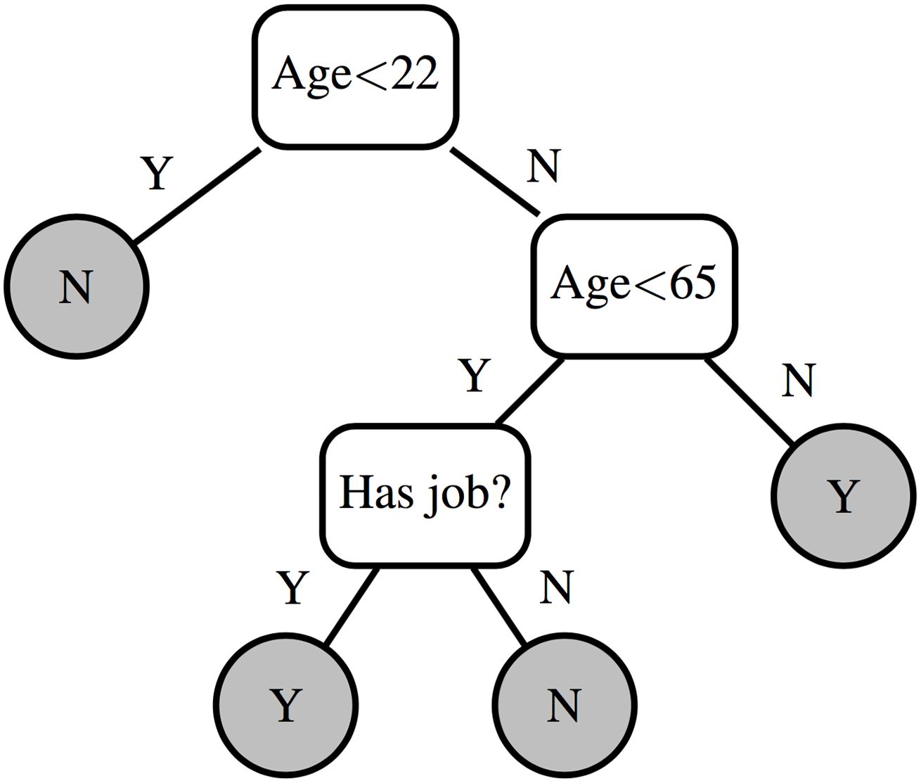
Figure 1 shows an example decision tree that can predict whether or not an individual owns a house. The decision is based on their age and whether or not they have a job. The tree correctly classifies all instances from Table 1.
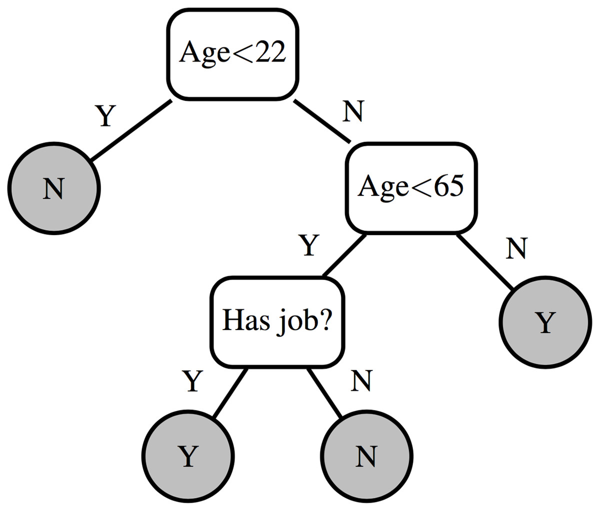
Figure 1: Example decision tree.
| Instance | Age | Has job | Owns house |
|---|---|---|---|
| 0 | 12 | N | N |
| 1 | 32 | Y | Y |
| 2 | 25 | Y | Y |
| 3 | 48 | N | N |
| 4 | 67 | N | Y |
| 5 | 18 | Y | N |
Decision tree algorithms typically expand nodes from the root in a greedy manner in order to maximise some criterion measuring the value of the split. For example, decision tree algorithms from the C4.5 family (Quinlan, 2014), designed for classification, use information gain as the split criterion. Information gain describes a change in entropy H from some previous state to a new state. Entropy is defined as where T is a set of labelled training instances, y ∈ Y is an instance label and P(y) is the probability of drawing an instance with label y from T. Information gain is defined as Here Tleft and Tright are the subsets of T created by a decision rule. ntotal, nleft and nright refer to the number of examples in the respective sets.
Many different criteria exist for evaluating the quality of a split. Any function can be used that produces some meaningful separation of the training instances with respect to the label being predicted.
In order to find the split that maximises our criterion, we can enumerate all possible splits on the input instances for each feature. In the case of numerical features and assuming the data has been sorted, this enumeration can be performed in O(nm) steps, where n is the number of instances and m is the number of features. A scan is performed from left to right on the sorted instances, maintaining a running sum of labels as the input to the gain calculation. We do not consider the case of categorical features in this paper because XGBoost encodes all categorical features using one-hot encoding and transforms them into numerical features.
Another consideration when building decision trees is how to perform regularisation to prevent overfitting. Overfitting on training data leads to poor model generalisation and poor performance on test data. Given a sufficiently large decision tree it is possible to generate unique decision rules for every instance in the training set such that each training instance is correctly labelled. This results in 100% accuracy on the training set but may perform poorly on new data. For this reason it is necessary to limit the growth of the tree during construction or apply pruning after construction.
Gradient boosting
Decision trees produce interpretable models that are useful for a variety of problems, but their accuracy can be considerably improved when many trees are combined into an ensemble model. For example, given an input instance to be classified, we can test it against many trees built on different subsets of the training set and return the mode of all predictions. This has the effect of reducing classifier error because it reduces variance in the estimate of the classifier.
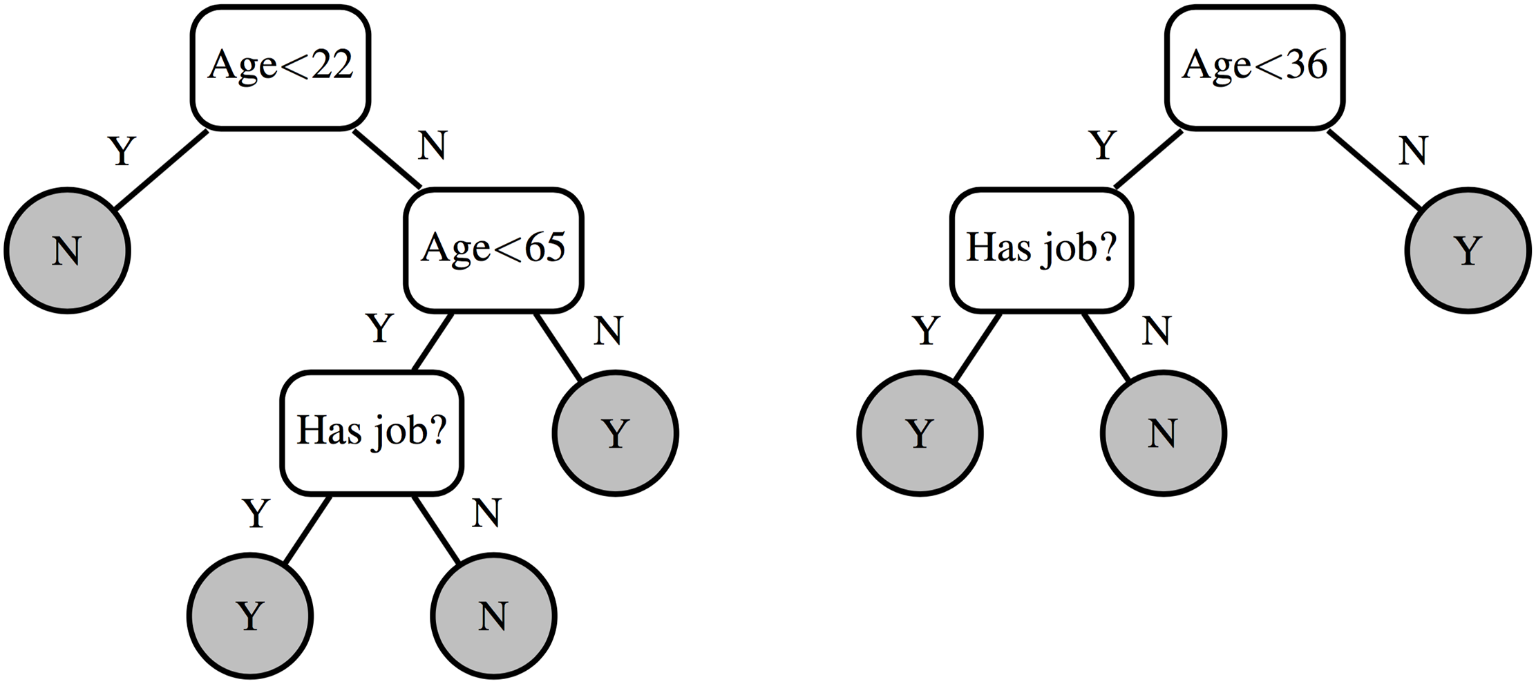
Figure 2 shows an ensemble of two decision trees. We can predict the output label using all trees by taking the most common class prediction or some weighted average of all predictions.
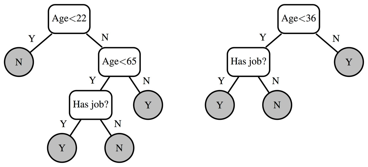
Figure 2: Decision tree ensemble.
Ensemble learning methods can also be used to reduce the bias component in the classification error of the base learner. Boosting is an ensemble method that creates ensemble members sequentially. The newest member is created to compensate for the instances incorrectly labelled by the previous learners.
Gradient boosting is a variation on boosting which represents the learning problem as gradient descent on some arbitrary differentiable loss function that measures the performance of the model on the training set. More specifically, the boosting algorithm executes M boosting iterations to learn a function F(x) that outputs predictions minimising some loss function . At each iteration we add a new estimator f(x) to try to correct the prediction of y for each training instance: We can correct the model by setting f(x) to: This fits the model f(x) for the current boosting iteration to the residuals y − Fm(x) of the previous iteration. In practice, we approximate f(x), for example by using a depth-limited decision tree.
This iterative process can be shown to be a gradient descent algorithm when the loss function is the squared error: To see this, consider that the loss over all training instances can be written as We seek to minimise J by adjusting F(xi). The gradient for a particular instance xi is given by We can see that the residuals are the negative gradient of the squared error loss function: By adding a model that approximates this negative gradient to the ensemble we move closer to a local minimum of the loss function, thus implementing gradient descent.
Generalised gradient boosting and XGBoost
Herein, we derive the XGBoost algorithm following the explanation in Chen & Guestrin (2016). XGBoost is a generalised gradient boosting implementation that includes a regularisation term, used to combat overfitting, as well as support for arbitrary differentiable loss functions.
Instead of optimising plain squared error loss, an objective function with two parts is defined, a loss function over the training set as well as a regularisation term which penalises the complexity of the model: can be any convex differentiable loss function that measures the difference between the prediction and true label for a given training instance. Ω(fk) describes the complexity of tree fk and is defined in the XGBoost algorithm (Chen & Guestrin, 2016) as (1) where T is the number of leaves of tree fk and w is the leaf weights (i.e. the predicted values stored at the leaf nodes). When Ω(fk) is included in the objective function we are forced to optimise for a less complex tree that simultaneously minimises . This helps to reduce overfitting. γT provides a constant penalty for each additional tree leaf and λw2 penalises extreme weights. γ and λ are user configurable parameters.
Given that boosting proceeds in an iterative manner we can state the objective function for the current iteration m in terms of the prediction of the previous iteration adjusted by the newest tree fk: We can then optimise to find the fk which minimises our objective.
Taking the Taylor expansion of the above function to the second order allows us to easily accommodate different loss functions: Here, gi and hi are the first and second order derivatives respectively of the loss function for instance i: Note that the model is left unchanged during this optimisation process. The simplified objective function with constants removed is We can also make the observation that a decision tree predicts constant values within a leaf. fk(x) can then be represented as wq(x) where w is the vector containing scores for each leaf and q(x) maps instance x to a leaf.
The objective function can then be modified to sum over the tree leaves and the regularisation term from Eq. (1): Here, Ij refers to the set of training instances in leaf j. The sums of the derivatives in each leaf can be defined as follows: Also note that wq(x) is a constant within each leaf and can be represented as wj. Simplifying we get (2) The weight wj for each leaf minimises the objective function at The best leaf weight wj given the current tree structure is then Using the best wj in Eq. (2), the objective function for finding the best tree structure then becomes (3) Eq. (3) is used in XGBoost as a measure of the quality of a given tree.
Growing a tree
Given that it is intractable to enumerate through all possible tree structures, we greedily expand the tree from the root node. In order to evaluate the usefulness of a given split, we can look at the contribution of a single leaf node j to the objective function from Eq. (3): We can then consider the contribution to the objective function from splitting this leaf into two leaves: The improvement to the objective function from creating the split is then defined as which yields (4) The quality of any given split separating a set of training instances is evaluated using the gain function in Eq. (4). The gain function represents the reduction in the objective function from Eq. (3) obtained by taking a single leaf node j and partitioning it into two leaf nodes. This can be thought of as the increase in quality of the tree obtained by creating the left and right branch as compared to simply retaining the original node. This formula is applied at every possible split point and we expand the split with maximum gain. We can continue to grow the tree while this gain value is positive. The γ regularisation cost at each leaf will prevent the tree arbitrarily expanding. The split point selection is performed in O(nm) time (given n training instances and m features) by scanning left to right through all feature values in a leaf in sorted order. A running sum of GL and HL is kept as we move from left to right, as shown in Table 3. GR and HR are inferred from this running sum and the node total.
Table 2 shows an example set of instances in a leaf. We can assume we know the sums G and H within this node as these are simply the GL or GR from the parent split. Therefore, we have everything we need to evaluate Gain for every possible split within these instances and select the best.
| Feature value | 0.1 | 0.4 | 0.5 | 0.6 | 0.9 | 1.1 |
|---|---|---|---|---|---|---|
| gi | 0.1 | 0.8 | 0.2 | −1.1 | −0.2 | −0.5 |
| hi | 1.0 | 1.0 | 1.0 | 1.0 | 1.0 | 1.0 |
| GL | 0.0 | 0.1 | 0.9 | 1.1 | 0.0 | −0.2 |
| HL | 0.0 | 1.0 | 2.0 | 3.0 | 4.0 | 5.0 |
XGBoost: data format
Tabular data input to a machine learning library such as XGBoost or Weka (Hall et al., 2009) can be typically described as a matrix with each row representing an instance and each column representing a feature as shown in Table 3. If f2 is the feature to be predicted then an input training pair takes the form ((f0i, f1i), f2i) where i is the instance id. A data matrix within XGBoost may also contain missing values. One of the key features of XGBoost is the ability to store data in a sparse format by implicitly keeping track of missing values instead of physically storing them. While XGBoost does not directly support categorical variables, the ability to efficiently store and process sparse input matrices allows us to process categorical variables through one-hot encoding. Table 4 shows an example where a categorical feature with three values is instead encoded as three binary features. The zeros in a one-hot encoded data matrix can be stored as missing values. XGBoost users may specify values to be considered as missing in the input matrix or directly input sparse formats such as libsvm files to the algorithm.
| Instance id | f0 | f1 | f2 |
|---|---|---|---|
| 0 | 0.32 | 399 | 10.1 |
| 1 | 0.27 | 521 | 11.3 |
| 2 | 0.56 | 896 | 13.0 |
| 3 | 0.11 | 322 | 9.7 |
| Instance id | f0 | f1 | f2 |
|---|---|---|---|
| 0 | 1 | 0 | 0 |
| 1 | 1 | 0 | 0 |
| 2 | 0 | 0 | 1 |
| 3 | 0 | 1 | 0 |
XGBoost: handling missing values
Representing input data using sparsity in this way has implications on how splits are calculated. XGBoost’s default method of handling missing data when learning decision tree splits is to find the best ‘missing direction’ in addition to the normal threshold decision rule for numerical values. So a decision rule in a tree now contains a numeric decision rule such as f0 ≤ 5.53, but also a missing direction such as missing = right that sends all missing values down the right branch. For a one-hot encoded categorical variable where the zeros are encoded as missing values, this is equivalent to testing ‘one vs all’ splits for each category of the categorical variable.
The missing direction is selected as the direction which maximises the gain from Eq. (4). When enumerating through all possible split values, we can also test the effect on our gain function of sending all missing examples down the left or right branch and select the best option. This makes split selection slightly more complex as we do not know the gradient statistics of the missing values for any given feature we are working on, although we do know the sum of all the gradient statistics for the current node. The XGBoost algorithm handles this by performing two scans over the input data, the second being in the reverse direction. In the first left to right scan the gradient statistics for the left direction are the scan values maintained by the scan, the gradient statistics for the right direction are the sum gradient statistics for this node minus the scan values. Hence, the right direction implicitly includes all of the missing values. When scanning from right to left, the reverse is true and the left direction includes all of the missing values. The algorithm then selects the best split from either the forwards or backwards scan.
Graphics processing units
The purpose of this paper is to describe how to efficiently implement decision tree learning for XGBoost on a GPU. GPUs can be thought of at a high level as having a shared memory architecture with multiple SIMD (single instruction multiple data) processors. These SIMD processors operate in lockstep typically in batches of 32 ‘threads’ (Matloff, 2011). GPUs are optimised for high throughput and work to hide latency through the use of massive parallelism. This is in contrast to CPUs which use multiple caches, branch prediction and speculative execution in order to optimise latency with regards to data dependencies (Baxter, 2013). GPUs have been used to accelerate a variety of tasks traditionally run on CPUs, providing significant speedups for parallelisable problems with a high arithmetic intensity. Of particular relevance to machine learning is the use of GPUs to train extremely large neural networks. It was shown in 2013 that one billion parameter networks could be trained in a few days on three GPU machines (Coates et al., 2013).
Languages and libraries
The two main languages for general purpose GPU programming are CUDA and OpenCL. CUDA was chosen for the implementation discussed in this paper due to the availability of optimised and production ready libraries. The GPU tree construction algorithm would not be possible without a strong parallel primitives library. We make extensive use of scan, reduce and radix sort primitives from the CUB (Merrill & NVIDIA-Labs, 2016) and Thrust (Hoberock & Bell, 2017) libraries. These parallel primitives are described in detail in ‘Parallel primitives.’ The closest equivalent to these libraries in OpenCL is the boost compute library. Several problems were encountered when attempting to use Boost Compute and the performance of its sorting primitives lagged considerably behind those of CUB/Thrust. At the time of writing this paper OpenCL was not a practical option for this type of algorithm.
Execution model
CUDA code is written as a kernel to be executed by many thousands of threads. All threads execute the same kernel function but their behaviour may be distinguished through a unique thread ID. Listing 1 shows an example of kernel adding values from two arrays into an output array. Indexing is determined by the global thread ID and any unused threads are masked off with a branch statement.
Threads are grouped according to thread blocks that typically each contain some multiple of 32 threads. A group of 32 threads is known as a warp. Thread blocks are queued for execution on hardware streaming multiprocessors. Streaming multiprocessors switch between different warps within a block during program execution in order to hide latency. Global memory latency may be hundreds of cycles and hence it is important to launch sufficiently many warps within a thread block to facilitate latency hiding.
A thread block provides no guarantees about the order of thread execution unless explicit memory synchronisation barriers are used. Synchronisation across thread blocks is not generally possible within a single kernel launch. Device-wide synchronisation is achieved by multiple kernel launches. For example, if a global synchronisation barrier is required within a kernel, the kernel must be separated into two distinct kernels where synchronisation occurs between the kernel launches.
Memory architecture
CUDA exposes three primary tiers of memory for reading and writing. Device-wide global memory, thread block accessible shared memory and thread local registers.
Global memory: Global memory is accessible by all threads and has the highest latency. Input data, output data and large amounts of working memory are typically stored in global memory. Global memory can be copied from the device (i.e. the GPU) to the host computer and vice versa. Bandwidth of host/device transfers is much slower than that of device/device transfers and should be avoided if possible. Global memory is accessed in 128 byte cache lines on current GPUs. Memory accesses should be coalesced in order to achieve maximum bandwidth. Coalescing refers to the grouping of aligned memory load/store operations into a single transaction. For example, a fully coalesced memory read occurs when a warp of 32 threads loads 32 contiguous 4 byte words (128 bytes). Fully uncoalesced reads (typical of gather operations) can limit device bandwidth to less than 10% of peak bandwidth (Harris, 2013).
Shared memory: 48 KB of shared memory is available to each thread block. Shared memory is accessible by all threads in the block and has a significantly lower latency than global memory. It is typically used as working storage within a thread block and sometimes described as a ‘programmer-managed cache.’
Registers: A finite number of local registers is available to each thread. Operations on registers are generally the fastest. Threads within the same warp may read/write registers from other threads in the warp through intrinsic instructions such as shuffle or broadcast (Nvidia, 2017).
Parallel primitives
Graphics processing unit primitives are small algorithms used as building blocks in massively parallel algorithms. While many data parallel tasks can be expressed with simple programs without them, GPU primitives may be used to compose more complicated algorithms while retaining high performance, readability and reliability. Understanding which specific tasks can be achieved using parallel primitives and the relative performance of GPU primitives as compared to their CPU counterparts is key to designing effective GPU algorithms.
Reduction
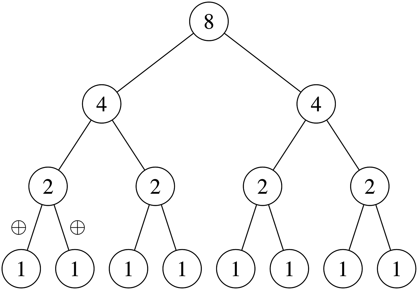
A parallel reduction reduces an array of values into a single value using a binary-associative operator. Given a binary-associative operator ⊕ and an array of elements the reduction returns . Note that floating point addition is not strictly associative. This means a sequential reduction operation will likely result in a different answer to a parallel reduction (the same applies to the scan operation described below). This is discussed in greater detail in ‘Floating point precision.’ The reduction operation is easy to implement in parallel by passing partial reductions up a tree, taking O(logn) iterations given n input items and n processors. This is illustrated in Fig. 3.
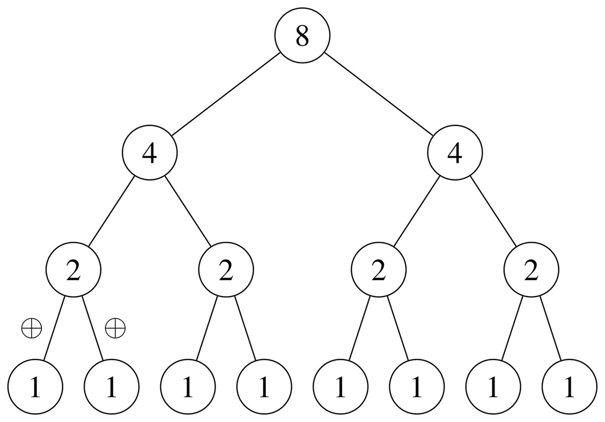
Figure 3: Sum parallel reduction.
In practice, GPU implementations of reductions do not launch one thread per input item but instead perform parallel reductions over ‘tiles’ of input items then sum the tiles together sequentially. The size of a tile varies according to the optimal granularity for a given hardware architecture. Reductions are also typically tiered into three layers: warp, block and kernel. Individual warps can very efficiently perform partial reductions over 32 items using shuffle instructions introduced from Nvidia’s Kepler GPU architecture onwards. As smaller reductions can be combined into larger reductions by simply applying the binary associative operator on the outputs, these smaller warp reductions can be combined together to get the reduction for the entire tile. The thread block can iterate over many input tiles sequentially, summing the reduction from each. When all thread blocks are finished the results from each are summed together at the kernel level to produce the final output. Listing 2 shows code for a fast warp reduction using shuffle intrinsics to communicate between threads in the same warp. The ‘shuffle down’ instruction referred to in Listing 2 simply allows the current thread to read a register value from the thread d places to the left, so long as that thread is in the same warp. The complete warp reduction algorithm requires five iterations to sum over 32 items.
Reductions are highly efficient operations on GPUs. An implementation is given in Harris (2007) that approaches the maximum bandwidth of the device tested.
Parallel prefix sum (scan)
The prefix sum takes a binary associative operator (most commonly addition) and applies it to an array of elements. Given a binary associative operator ⊕ and an array of elements the prefix sum returns . A prefix sum is an example of a calculation which seems inherently serial but has an efficient parallel algorithm: the Blelloch scan algorithm.
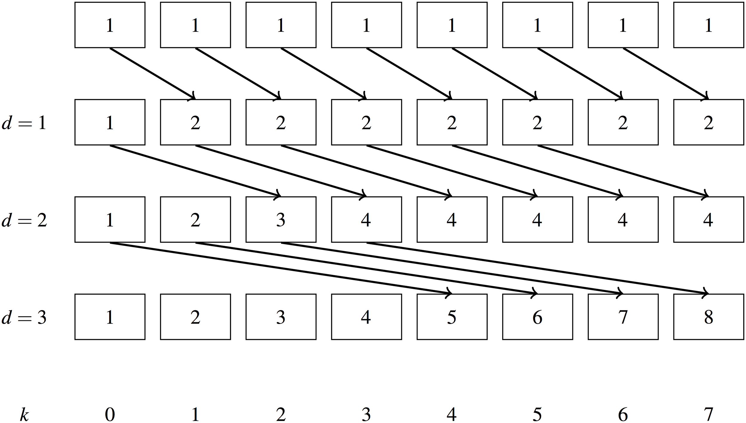
Let us consider a simple implementation of a parallel scan first, as described in Hillis & Steele (1986). It is given in Algorithm 1. Figure 4 shows it in operation: we apply a simple scan with the addition operator to an array of 1’s. Given one thread for each input element the scan takes iterations to complete. The algorithm performs O(nlog2n) addition operations.
| 1 | for d=1 to log2n do |
| 2 | for k=0 to n−1 in parallel do |
| 3 | if k ≥ 2d−1 then |
| 4 | x[k] := x[k − 2d−1] + x[k] |
| 5 | end |
| 6 | end |
| 7 | end |
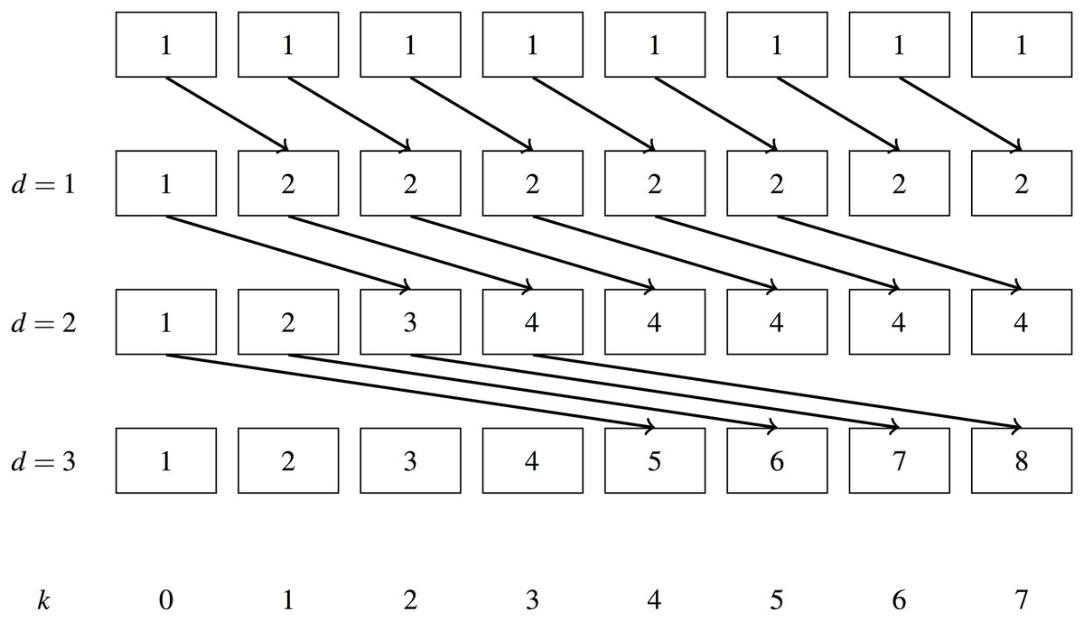
Figure 4: Simple parallel scan example.
Given that a sequential scan performs only n addition operations, the simple parallel scan is not work efficient. A work efficient parallel algorithm will perform the same number of operations as the sequential algorithm and may provide significantly better performance in practice. A work efficient algorithm is described in Blelloch (1990). The algorithm is separated into two phases, an ‘upsweep’ phase similar to a reduction and a ‘downsweep’ phase. We give pseudocode for the upsweep (Algorithm 2) and downsweep (Algorithm 3) phases by following the implementation in Harris, Sengupta & Owens (2007).
| 1 | offset = 1 |
| 2 | for d= log2 n to 1 do |
| 3 | for k=0 to n−1 in parallel do |
| 4 | if k < 2d−1 then |
| 5 | ai = offset × (2 × k + 1) − 1 |
| 6 | bi = offset × (2 × k + 2) − 1 |
| 7 | x[bi] = x[bi] + x[ai] |
| 8 | end |
| 9 | end |
| 10 | offset = offset * 2 |
| 11 | end |
| 1 | |
| 2 | x[n − 1] := 0 |
| 3 | for d=1 to log2n do |
| 4 | for k=0 to n−1 in parallel do |
| 5 | if k < 2d−1 then |
| 6 | ai = offset × (2 × k + 1) − 1 |
| 7 | bi = offset × (2 × k + 2) − 1 |
| 8 | t = x[ai] |
| 9 | x[ai] = x[bi] |
| 10 | x[bi] = x[bi] + t |
| 11 | end |
| 12 | end |
| 13 | offset = offset/2 |
| 14 | end |
Figures 5 and 6 show examples of the work efficient Blelloch scan, as an exclusive scan (the sum for a given item excludes the item itself). Solid lines show summation with the previous item in the array, dotted lines show replacement of the previous item with the new value. O(n) additions are performed in both the upsweep and downsweep phase resulting in the same work efficiency as the serial algorithm.
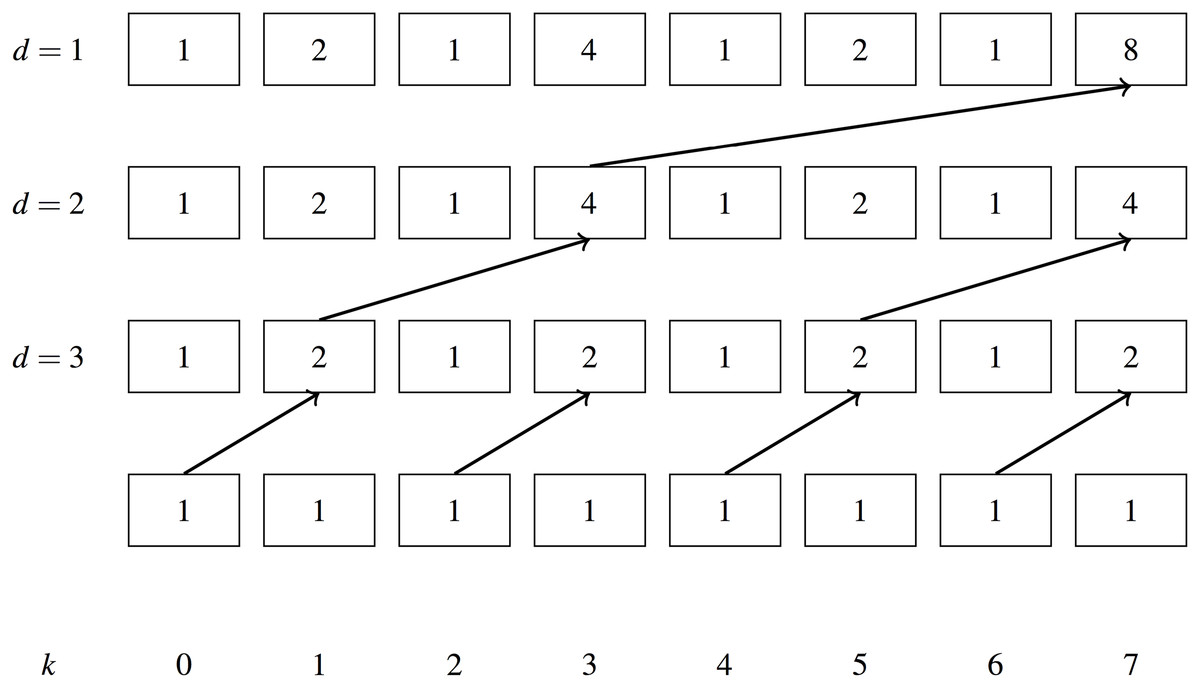
Figure 5: Blelloch scan upsweep example.
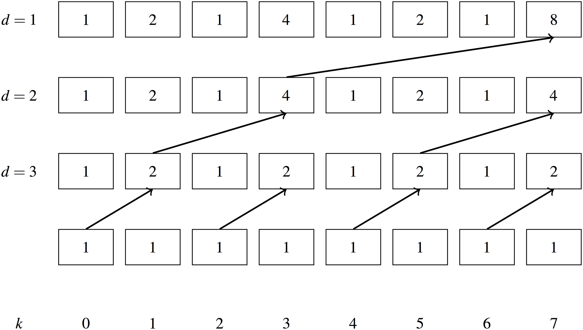

Figure 6: Blelloch scan downsweep example.
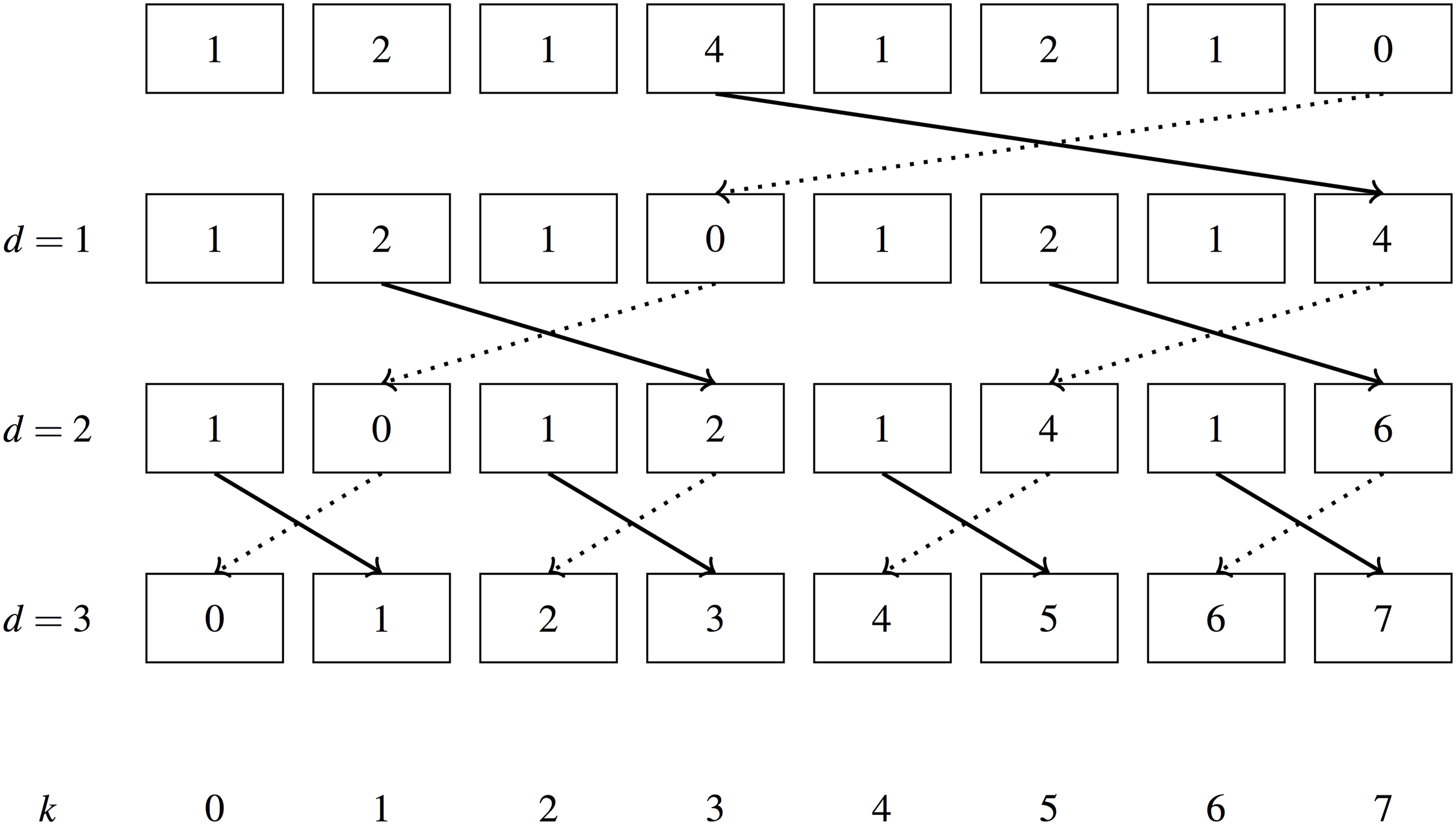
A segmented variation of scan that processes contiguous blocks of input items with different head flags can be easily formulated. This is achieved by creating a binary associative operator on key value pairs. The operator tests the equality of the keys and sums the values if they belong to the same sequence. This is discussed further in ‘Scan and reduce on multiple sequences.’
A scan may also be implemented using warp intrinsics to create fast 32 item prefix sums based on the simple scan in Fig. 4. Code for this is shown in Listing 3. Although the simple scan algorithm is not work efficient, we use this approach for small arrays of size 32.
Radix sort
Radix sorting on GPUs follows from the ability to perform parallel scans. A scan operation may be used to calculate the scatter offsets for items within a single radix digit as described in Algorithm 4 and Fig. 7. Flagging all ‘0’ digits with a one and performing an exclusive scan over these flags gives the new position of all zero digits. All ‘1’ digits must be placed after all ‘0’ digits, therefore the final positions of the ‘1’s can be calculated as the exclusive scan of the ‘1’s plus the total number of ‘0’s. The exclusive scan of ‘1’ digits does not need to be calculated as it can be inferred from the array index and the exclusive scan of ‘0’s. For example, at index 5 (using 0-based indexing), if our exclusive scan shows a sum of 3 ‘0’s, then there must be two ‘1’s because a digit can only be 0 or 1.
| Input :X | |
| Output :Y | |
| 1 | for i = 0 to n − 1 in parallel do |
| 2 | F[i] := bit_flip(X[i]) |
| 3 | end |
| 4 | S := exclusive_scan(F) |
| 5 | r := S[n − 1] + F[n − 1] |
| 6 | for i = 0 to n − 1 in parallel do |
| 7 | if X[i] = 0 then |
| 8 | A[i] := S[i] |
| 9 | else if X[i] = 1 then |
| 10 | A[i] := i − S[i] + r |
| 11 | end |
| 12 | for i = 0 to n − 1 in parallel do |
| 13 | Y[A[i]] := X[i] |
| 14 | end |

Figure 7: Radix sort example.
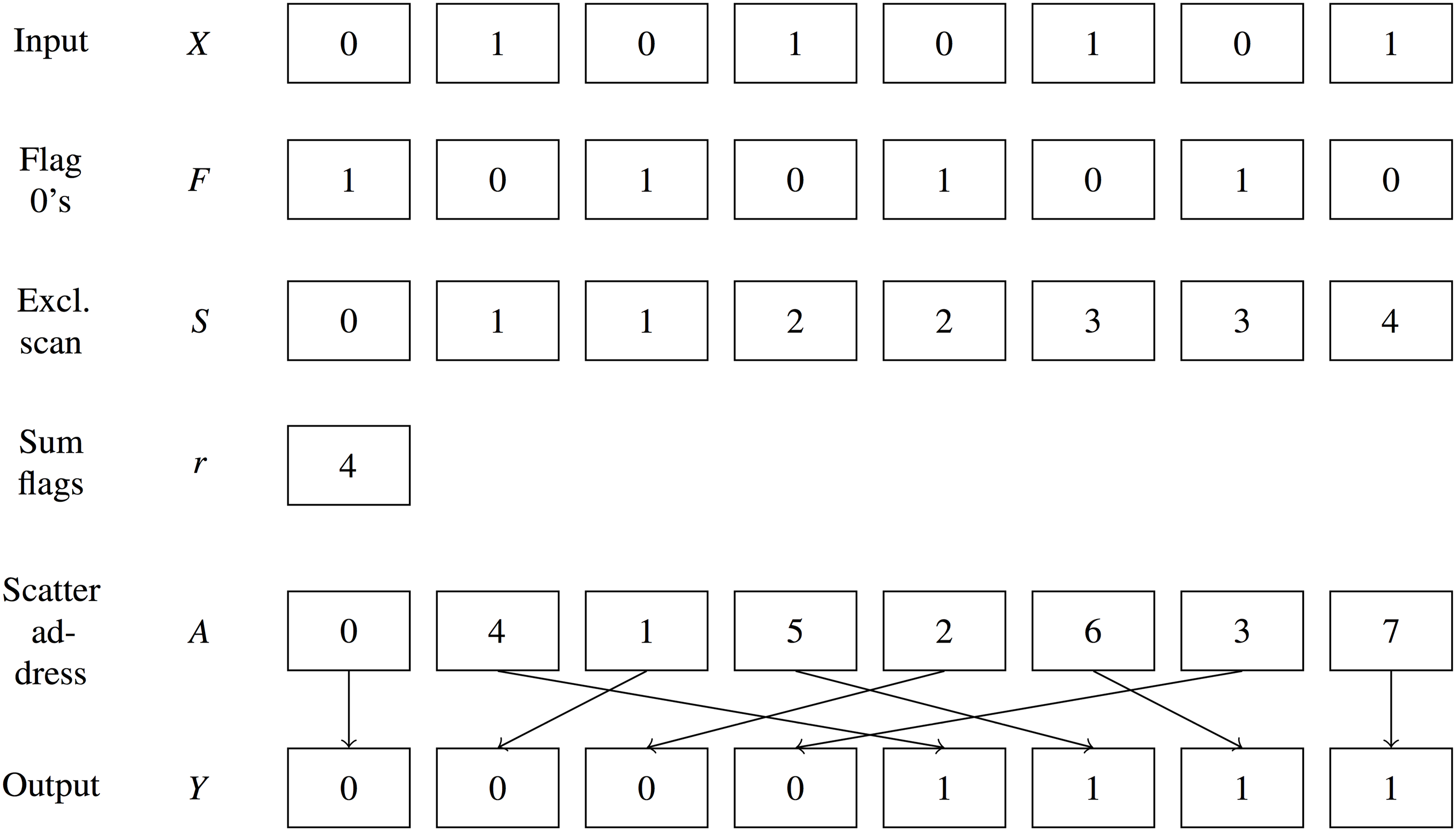
The basic radix sort implementation only sorts unsigned integers but this can be extended to correctly sort signed integers and floating point numbers through simple bitwise transformations. Fast implementations of GPU radix sort perform a scan over many radix bits in a single pass. Merrill & Grimshaw (2011) show a highly efficient and practical implementation of GPU radix sorting. They show speedups of 2× over a 32 core CPU and claim to have the fastest sorting implementation for any fully programmable microarchitecture.
Scan and reduce on multiple sequences
Variations on scan and reduce consider multiple sequences contained within the same input array and identified by key flags. This is useful for building decision trees as the data can be repartitioned into smaller and smaller groups as we build the tree.
We will describe an input array as containing either ‘interleaved’ or ‘segmented’ sequences. Table 5 shows an example of two interleaved sequences demarcated by flags. Its values are mixed up and do not reside contiguously in memory. This is in contrast to Table 6, with two ‘segmented’ sequences. The segmented sequences reside contiguously in memory.
| Sequence Id | 0 | 0 | 1 | 0 | 1 | 1 |
|---|---|---|---|---|---|---|
| Values | 1 | 1 | 1 | 1 | 1 | 1 |
| Values scan | 1 | 2 | 1 | 3 | 2 | 3 |
| Sequence Id | 0 | 0 | 0 | 1 | 1 | 1 |
|---|---|---|---|---|---|---|
| Values | 1 | 1 | 1 | 1 | 1 | 1 |
| Values scan | 1 | 2 | 3 | 1 | 2 | 3 |
Segmented scan
A scan can be performed on the sequences from Table 6 using the conventional scan algorithm described in ‘Parallel prefix sum (scan)’ by modifying the binary associative operator to accept key value pairs. Listing 4 shows an example of a binary associative operator that performs a segmented summation. It resets the sum when the key changes.
Segmented reduce
A segmented reduction can be implemented efficiently by applying the segmented scan described above and collecting the final value of each sequence. This is because the last element in a scan is equivalent to a reduction.
Interleaved sequences: multireduce
A reduction operation on interleaved sequences is commonly described as a multireduce operation. To perform a multireduce using the conventional tree algorithm described in ‘Reduction’ a vector of sums can be passed up the tree instead of a single value, with one sum for each unique sequence. As the number of unique sequences or ‘buckets’ increases, this algorithm becomes impractical due to limits on temporary storage (registers and shared memory).
A multireduce can alternatively be formulated as a histogram operation using atomic operations in shared memory. Atomic operations allow multiple threads to safely read/write a single piece of memory. A single vector of sums is kept in shared memory for the entire thread block. Each thread can then read an input value and increment the appropriate sum using atomic operations. When multiple threads contend for atomic read/write access on a single piece of memory they are serialised. Therefore, a histogram with only one bucket will result in the entire thread block being serialised (i.e. only one thread can operate at a time). As the number of buckets increases this contention is reduced. For this reason the histogram method will only be appropriate when the input sequences are distributed over a large number of buckets.
Interleaved sequences: multiscan
A scan operation performed on interleaved sequences is commonly described as a multiscan operation. A multiscan may be implemented, like multireduce, by passing a vector of sums as input to the binary associative operator. This increases the local storage requirements proportionally to the number of buckets.
General purpose multiscan for GPUs is discussed in Eilers (2014) with the conclusion that ‘multiscan cannot be recommended as a general building block for GPU algorithms.’ However, highly practical implementations exist that are efficient up to a limited number of interleaved buckets, where the vector of sums approach does not exceed the capacity of the device. The capacity of the device in this case refers to the amount of registers and shared memory available for each thread to store and process a vector.
Merill and Grimshaw’s optimised radix sort implementation (Merrill & NVIDIA-Labs, 2016; Merrill & Grimshaw, 2011), mentioned in ‘Radix sort,’ relies on an eight-way multiscan in order to calculate scatter addresses for up to 4 bits at a time in a single pass.
Floating point precision
The CPU implementation of the XGBoost algorithm represents gradient/Hessian pairs using two 32 bit floats. All intermediate summations are performed using 64 bit doubles to control loss of precision from floating point addition. This is problematic when using GPUs as the number of intermediate values involved in a reduction scales with the input size. Using doubles significantly increases the usage of scarce registers and shared memory; moreover, gaming GPUs are optimised for 32 bit floating point operations and give relatively poor double precision throughput.
Table 7 shows the theoretical GFLOPs of two cards we use for benchmarking. The single precision GFLOPs are calculated as 2× number of CUDA cores × core clock speed (in GHz), where the factor of 2 represents the number of operations per required FMA (fused-multiply-add) instruction. Both these cards have 32 times more single precision ALUs (arithmetic logic units) than double precision ALUs, resulting in 1/32 the theoretical double precision performance. Therefore, an algorithm relying on double precision arithmetic will have severely limited performance on these GPUs.
| GPU | Single precision | Double precision |
|---|---|---|
| GTX 970 (Maxwell) | 3,494 | 109 |
| Titan X (Pascal) | 10,157 | 317 |
We can test the loss of precision from 32 bit floating point operations to see if double precision is necessary by considering 32 bit parallel and sequential summation, summing over a large array of random numbers. Sequential double precision summation is used as the baseline, with the error measured as the absolute difference from the baseline. The experiment is performed over 10 million random numbers between −1 and 1, with 100 repeats. The mean error and standard deviation are reported in Table 8. The Thrust library is used for parallel GPU reduction based on single precision operations.
| Algorithm | Mean error | SD |
|---|---|---|
| Sequential | 0.0694 | 0.0520 |
| Parallel | 0.0007 | 0.0005 |
The 32 bit parallel summation shows dramatically superior numerical stability compared to the 32 bit sequential summation. This is because the error of parallel summation grows proportionally to O(logn), as compared to O(n) for sequential summation (Higham, 1993). The parallel reduction algorithm from Fig. 3 is commonly referred to as ‘pairwise summation’ in literature relating to floating point precision. The average error of 0.0007 over 10 million items shown in Table 8 is more than acceptable for the purposes of gradient boosting. The results also suggests that the sequential summation within the original XGBoost could be safely performed in single precision floats. A mean error of 0.0694 over 10 million items is very unlikely to be significant compared to the noise typically present in the training sets of supervised learning tasks.
Building tree classifiers on GPUs
Graphics processing unit-accelerated decision trees and forests have been studied as early as 2008 in Sharp (2008) for the purpose of object recognition, achieving speedups of up to 100× for this task. Decision forests were mapped to a 2-D texture array and trained/evaluated using GPU pixel and vertex shaders. A more general purpose random forest implementation is described in Grahn et al. (2011) showing speedups of up to 30× over state-of-the-art CPU implementations for large numbers of trees. The authors use an approach where one GPU thread is launched to construct each tree in the ensemble.
A decision tree construction algorithm using CUDA based on the SPRINT decision tree inducer is described in Chiu, Luo & Yuan (2011). No performance results are reported. Another decision tree construction algorithm is described in Lo et al. (2014). They report speedups of 5–55× over WEKA’s Java-based implementation of C4.5 (Quinlan, 2014), called J48, and 18× over SPRINT. Their algorithm processes one node at a time and as a result scales poorly at higher tree depths due to higher per-node overhead as compared to a CPU algorithm.
Nasridinov, Lee & Park (2014) describe a GPU-accelerated algorithm for ID3 decision tree construction, showing moderate speedups over WEKA’s ID3 implementation. Nodes are processed one at a time and instances are resorted at every node. Strnad & Nerat (2016) devise a decision tree construction algorithm that stores batches of nodes in a work queue on the host and processes these units of work on the GPU. They achieve speedups of between 2× and 7× on large data sets as compared to a multithreaded CPU implementation. Instances are resorted at every node (Strnad & Nerat, 2016).
Our work has a combination of key features differentiating it from these previous approaches. First, our implementation processes all nodes in a level concurrently, allowing it to scale beyond trivial depths with near constant run-time. A GPU tree construction algorithm that processes one node at a time will incur a nontrivial constant kernel launch overhead for each node processed. Additionally, as the training set is recursively partitioned at each level, the average number of training examples in each node decreases rapidly. Processing a small number of training examples in a single GPU kernel will severely underutilise the device. This means the run-time increases dramatically with tree depth. To achieve state-of-the-art results in data mining competitions we found that users very commonly required tree depths of greater than 10 in XGBoost. This contradicts the conventional wisdom that a tree depth of between 4 and 8 is sufficient for most boosting applications (Friedman, Hastie & Tibshirani, 2001). Our approach of processing all nodes on a level concurrently is far more practical in this setting.
Secondly, our decision tree implementation is not a hybrid CPU/GPU approach and so does not use the CPU for computation. We find that all stages of the tree construction algorithm can be efficiently completed on the GPU. This was a conscious design decision in order to reduce the bottleneck of host/device memory transfers. At the time of writing, host/device transfers are limited to approximately 16 GB/s by the bandwidth of the Gen 3 PCIe standard. The Titan X GPU we use for benchmarking has an on-device memory bandwidth of 480 GB/s, a factor of 30 times greater. Consequently, applications that move data back and forward between the host and device will not be able to achieve peak performance. Building the entire decision tree in device memory has the disadvantage that the device often has significantly lower memory capacity than the host. Despite this, we show that it is possible to process some very large benchmark datasets entirely in device memory on a commodity GPU.
Thirdly, our algorithm implements the sparsity aware tree construction method introduced by XGBoost. This allows it to efficiently process sparse input matrices in terms of run-time and memory usage. This is in contrast to previous GPU tree construction algorithms. Additionally, our implementation is provided as a part of a fully featured machine learning library. It implements regression, binary classification, multiclass classification and ranking through the generalised gradient boosting framework of XGBoost and has an active user base. No published implementations exist for any of the existing GPU tree construction algorithms described above, making direct comparison to the approach presented in this work infeasible.
Parallel Tree Construction
Our algorithm builds a single decision tree for a boosting iteration by processing decision tree nodes in a level-wise manner. At each level we search for the best split within each leaf node, update the positions of training instances based on these new splits and then repartition data if necessary. Processing an entire level at a time allows us to saturate the GPU with the maximum amount of work available in a single iteration. Our algorithm performs the following three high level phases for each tree level until the maximum tree depth is reached: (1) find splits, (2) update node positions, and (3) sort node buckets (if necessary).
Phase 1: find splits
The first phase of the algorithm finds the best split for each leaf node at the current level.
Data layout
To facilitate enumeration through all split points, the feature values should be kept in sorted order. Hence, we use the device memory layout shown in Tables 9 and 10. Each feature value is paired with the ID of the instance it belongs to as well as the leaf node it currently resides in. Data are stored in sparse column major format and instance IDs are used to map back to gradient pairs for each instance. All data are stored in arrays in device memory. The tree itself can be stored in a fixed length device array as it is strictly binary and has a maximum depth known ahead of time.
| f0 | f1 | f2 | ||||||
|---|---|---|---|---|---|---|---|---|
| Node id | 0 | 0 | 0 | 0 | 0 | 0 | 0 | 0 |
| Instance id | 0 | 2 | 3 | 3 | 2 | 0 | 1 | 3 |
| Feature value | 0.1 | 0.5 | 0.9 | 5.2 | 3.1 | 3.6 | 3.9 | 4.7 |
| Instance id | 0 | 1 | 2 | 3 |
| Gradient pair | p0 | p1 | p2 | p3 |
Block level parallelism
Given the above data layout notice that each feature resides in a contiguous block and may be processed independently. In order to calculate the best split for the root node of the tree, we greedily select the best split within each feature, delegating a single thread block per feature. The best splits for each feature are then written out to global memory and are reduced by a second kernel. A downside of this approach is that when the number of features is not enough to saturate the number of streaming multiprocessors—the hardware units responsible for executing a thread block—the device will not be fully utilised.
Calculating splits
In order to calculate the best split for a given feature we evaluate Eq. (4) at each possible split location. This depends on (GL, HL) and (GR, HR). We obtain (GL, HL) from a parallel scan of gradient pairs associated with each feature value. (GR, HR) can be obtained by subtracting (GL, HL) from the node total which we know from the parent node.
The thread block moves from left to right across a given feature, consuming ‘tiles’ of input. A tile herein refers to the set of input items able to be processed by a thread block in one iteration. Table 11 gives an example of a thread block with four threads evaluating a tile with four items. For a given tile, gradient pairs are scanned and all splits are evaluated.
| Thread block 0 | ⇒ | |||||||
|---|---|---|---|---|---|---|---|---|
| ↓ | ↓ | ↓ | ↓ | |||||
| f0 | ||||||||
| Instance id | 0 | 2 | 3 | 1 | 7 | 5 | 6 | 4 |
| Feature value | 0.1 | 0.2 | 0.3 | 0.5 | 0.5 | 0.7 | 0.8 | 0.8 |
| Gradient pair | p0 | p2 | p3 | p1 | p7 | p5 | p6 | p4 |
Each 32 thread warp performs a reduction to find the best local split and keeps track of the current best feature value and accompanying gradient statistics in shared memory. At the end of processing the feature, another reduction is performed over all the warps’ best items to find the best split for the feature.
Missing values
The original XGBoost algorithm accounts for missing values by scanning through the input values twice as described in ‘XGBoost: handling missing values’—once in the forwards direction and once in the reverse direction. An alternative method used by our GPU algorithm is to perform a sum reduction over the entire feature before scanning. The gradient statistics for the missing values can then be calculated as the node sum statistics minus the reduction. If the sum of the gradient pairs from the missing values is known, only a single scan is then required. This method was chosen as the cost of a reduction can be significantly less than performing the second scan.
Node buckets
So far the algorithm description only explains how to find a split at the first level where all instances are bucketed into a single node. A decision tree algorithm must, by definition, separate instances into different nodes and then evaluate splits over these subsets of instances. This leaves us with two possible options for processing nodes. The first is to leave all data instances in their current location, keeping track of which node they currently reside in using an auxiliary array as shown in Table 12. When we perform a scan across all data values we keep temporary statistics for each node. We therefore scan across the array processing all instances as they are interleaved with respect to their node buckets. This is the method used by the CPU XGBoost algorithm. We also perform this method on the GPU, but only to tree depths of around 5. This interleaved algorithm is fully described in ‘Interleaved algorithm: finding a split.’
| f0 | f1 | f2 | ||||||
|---|---|---|---|---|---|---|---|---|
| Node id | 2 | 1 | 2 | 2 | 1 | 2 | 1 | 2 |
| Instance id | 0 | 2 | 3 | 3 | 2 | 0 | 1 | 3 |
| Feature value | 0.1 | 0.5 | 0.9 | 5.2 | 3.1 | 3.6 | 3.9 | 4.7 |
The second option is to radix sort instances by their node buckets at each level in the tree. This second option is described fully in ‘Sorting algorithm: finding a split.’ Briefly, data values are first ordered by their current node and then by feature values within their node buckets as shown in Table 13. This transforms the interleaved scan (‘multiscan’) problem described above into a segmented scan, which has constant temporary storage requirements and thus scales to arbitrary depths in a GPU implementation.
| f0 | f1 | f2 | ||||||
|---|---|---|---|---|---|---|---|---|
| Node id | 1 | 2 | 2 | 1 | 2 | |||
| Instance id | 0 | 2 | 3 | 3 | 2 | 1 | 0 | 3 |
| Feature value | 0.5 | 0.1 | 0.9 | 5.2 | 3.1 | 3.9 | 3.6 | 4.7 |
In our implementation, we use the interleaved method for trees of up to depth 5 and then switch to the sorting version of the algorithm. Avoiding the expensive radix sorting step for as long as possible can provide speed advantages, particularly when building small trees. The maximum number of leaves at depth 5 is 32. At greater depths there are insufficient shared memory resources and the exponentially increasing run-time begins to be uncompetitive.
Interleaved algorithm: finding a split
In order to correctly account for missing values a multireduce operation must be performed to obtain the sums within interleaved sequences of nodes. A multiscan is then performed over gradient pairs. Following that, unique feature values are identified and gain values calculated to identify the best split for each node. We first discuss the multireduce and multiscan operations before considering how to evaluate splits.
Multireduce and multiscan
Algorithms 5 and 6 outline the approach used for multireduce/multiscan at the thread block level. Our multiscan/multireduce approach is formulated around sequentially executing fast warp synchronous scan/reduce operations for each bucket. Passing vectors of items to the binary associative operator is not generally possible given the number of buckets and the limited temporary storage. This was discussed in ‘Scan and reduce on multiple sequences.’ We instead perform warp level multiscan operations. Listing 5 shows how a 32-thread warp can perform a multiscan by masking off non-active node buckets and performing a normal warp scan for each node bucket. The function ‘WarpExclusiveScan()’ herein refers to an exclusive version of the warp scan described in Listing 3.
| 1. | An input tile is loaded. |
| 2. | Each warp performs local reduction for each bucket, masking off items for the current bucket. |
| 3. | Each warp adds its local reductions into shared memory. |
| 4. | The remaining tiles are processed. |
| 5. | The partial sums in shared memory are reduced by a single warp into the final node sums. |
| 1. | An input tile is loaded. |
| 2. | Each warp performs local scans for each bucket, masking off items for the current bucket. |
| 3. | The sums from each local scan are placed into shared memory. |
| 4. | The partial sums in shared memory are scanned. |
| 5. | The scanned partial sums in shared memory are added back into the local values. |
| 6. | The running sum from the previous tile is added to the local values. |
| 7. | The remaining tiles are processed. |
Note that the number of warp reductions/scans performed over a warp of data increases exponentially with tree depth. This leads to an exponentially increasing run time relative to the depth of the tree, but is surprisingly performant even up to depth 6 as warp synchronous reductions/scans using shuffle instructions are cheap to compute. They only perform operations on registers and incur no high latency reads or writes into global memory.
The exclusive scan for the entire input tile is calculated from individual warp scans by performing the same multiscan operation over the sums of each warp scan and scattering the results of this back into each item. More detailed information on how to calculate a block-wide scan from smaller warp scan operations is given in Nvidia (2016).
Evaluating splits
There is one additional problem that must be solved. It arises as a consequence of processing node buckets in interleaved order. In a decision tree algorithm, when enumerating through feature values to find a split, we should not choose a split that falls between two elements with the same value. This is because a decision rule will not be able to separate elements with the same value. For a value to be considered as a split, the corresponding item must be the leftmost item with that feature value for that particular node (we could also arbitrarily take the rightmost value).
Because the node buckets are interleaved, it is not possible to simply check the item to the left to see if the feature value is the same—the item to the left of a given item may reside in a different node. To check if an item with a certain feature value is the leftmost item with that value in its node bucket, we can formulate a scan with a special binary associative operator. First, each item is assigned a bit vector of length n + 1 where n is the number of buckets. If the item resides within bucket i then xi will be set to 1. If the item’s feature value is distinct from the value of the item directly to the left (irrespective of bucket) then xn+1 is set to 1. All other bits are set to 0.
We can then define a binary associative operator as follows: (5)
Bit xn+1 acts as a segmentation flag, resetting the scan so many small scans are performed across groups of items with the same feature value. Scanning the bucket flags with a logical or operator determines which node buckets are represented in the items to the left of the current item. Therefore, within a group of items with the same feature value, if the current item’s bucket flag is set to 0 for the bucket it resides in, the item represents the leftmost item with that value in its bucket. This item can then be used as a split point.
In practice, a 64 bit integer is used as the bit vector in order to hold a maximum of 33 bits at the sixth level of the tree (the maximum number of active nodes at this level +1 for the segmentation flag). The operator is formulated according to Listing 6 in C++ code. Moreover, when applying this interleaved algorithm we cannot choose the split value as the halfway point between two training examples: We do not know the value of the item to the left within the current node, only if it is the same as the current item or not. The split value is accordingly calculated as the current value minus some small constant. This distinction in the split value does not affect accuracy in practice.
Complete algorithm
Given a reduction, scan and the above method for finding unique feature values we have all the machinery necessary to enumerate splits and select the best. The complete algorithm for a thread block processing a single feature at a given tree level is shown in Algorithm 7.
| 1. | Load input tile |
| 2. | Multireduce tile gradient pairs |
| 3. | Go to 1. until all tiles processed |
| 4. | Return to first tile |
| 5. | Load input tile |
| 6. | Multiscan tile gradient pairs |
| 7. | Scan tile for unique feature values |
| 8. | Calculate gain for each split |
| 9. | Store best split for each warp |
| 10. | Go to 5. until all tiles processed |
| 11. | Output best splits |
The output of this algorithm contains the best split for each leaf node for a given feature. Each thread block outputs the best splits for its assigned feature. These splits are then further reduced by a global kernel to find the best splits for any feature.
Sorting algorithm: finding a split
The sorting implementation of the split finding algorithm operates on feature value data grouped into node buckets. Given data sorted by node ID first and then feature values second we can perform segmented scan/reduce operations over an entire feature only needing a constant amount of temporary storage.
The segmented reduction to find gradient pair sums for each node is implemented as a segmented sum scan, storing the final element from each segment as the node sum. Another segmented scan is then performed over the input feature to get the exclusive scan of gradient pairs. After scanning each tile, the split gain is calculated using the scan and reduction as input and the best splits are stored in shared memory.
The segmented scan is formulated by performing an ordinary scan over key value pairs with a binary associative operator that resets the sum when the key changes. In this case the key is the current node bucket and the value is the gradient pair. The operator is shown in Eq. (6).
(6)An overview of the split finding algorithm for a single thread block processing a feature is provided in Algorithm 8. The output of this algorithm, like that of the interleaved algorithm, consists of the best splits for each feature, and each node. This is reduced by a global kernel to find the best splits for each node, of any feature.
| 1. | Load input tile |
| 2. | Segmented reduction over tile gradient pairs |
| 3. | Go to 1. until all tiles processed |
| 4. | Return to first tile |
| 5. | Load input tile |
| 6. | Segmented scan over tile gradient pairs |
| 7. | Calculate gain for each split |
| 8. | Store best split for each warp |
| 9. | Go to 5. until all tiles processed |
| 10. | Output best splits |
Phase 2: update node positions
Once the best splits for each node have been calculated, the node positions for each instance must be updated. This is made non-trivial because of the presence of missing values. We first create an array containing the pre-split node position of each training instance. These node positions are then updated as if they contained all missing values, according to the default missing direction in the newly calculated splits. We then update this array again based on the feature values of the instances. Any instance which does not have a value for that feature (missing value) will have its node position left unchanged as per the missing direction. Because we now have the updated node position for each instance, we write these node positions back to each feature value.
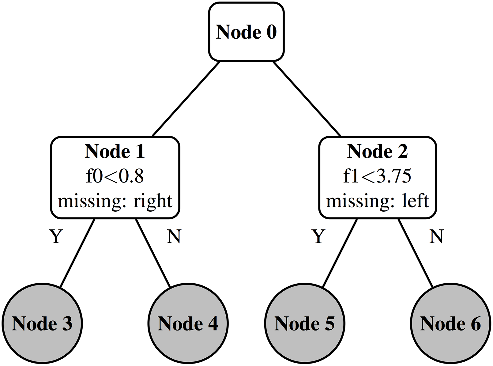
To illustrate this with an example, Fig. 8 shows the state of a decision tree after having calculated splits for level 1. The node positions in the data structure used for split finding (Table 14) must be updated before proceeding to calculate the splits for level 2. To do this we update the array in Table 15 that maps instances to a node.
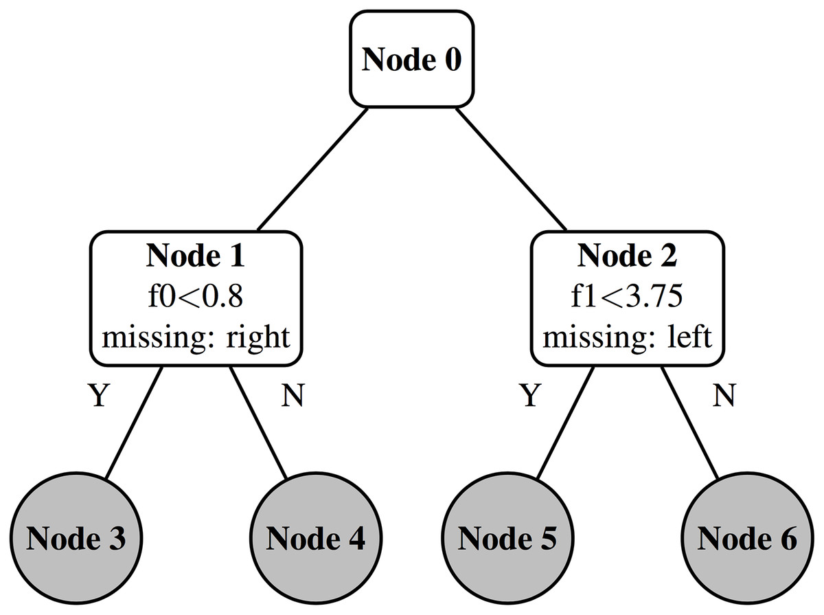
Figure 8: Decision tree: four new leaves.
| f0 | f1 | ||||||
|---|---|---|---|---|---|---|---|
| Node id | 1 | 2 | 2 | 1 | 1 | 2 | 2 |
| Instance id | 0 | 2 | 1 | 3 | 0 | 1 | 2 |
| Feature value | 0.75 | 0.5 | 0.9 | 2.7 | 4.1 | 3.6 | 3.9 |
First we update the node ID map in the missing direction. All instances residing in node 1 are updated in the right direction to node 4. Instances residing in node 2 are updated in the left direction to node 5. The node ID map now looks like Table 16.
| Instance id | 0 | 1 | 2 | 3 |
| Node id | 4 | 5 | 5 | 4 |
We now update the map again using the feature values from Table 14, overwriting the previous values. Instance 0 resides in node 1 so we check if f0 < 0.8. This is true so instance 0 moves down the left branch into node 3. Instance 1 moves into node 5 and instance 2 moves into node 6 based on their f1 values. Note that instance 3 has a missing value for f0. Its node position is therefore kept as the missing direction updated in the previous step. This process is shown in Table 17.
| Instance id | 0 | 1 | 2 | 3 | ||||
| Node id | 3 | 5 | 6 | 4 |
| f0 | f1 | ||||||
|---|---|---|---|---|---|---|---|
| Node id | 1 | 2 | 2 | 1 | 1 | 2 | 2 |
| Instance id | 0 | 2 | 1 | 3 | 1 | 1 | 2 |
| Feature value | 0.75 | 0.5 | 0.9 | 2.7 | 4.1 | 3.6 | 3.9 |
The per instance node ID array is now up-to-date for the new level so we write these values back into the per feature value array, giving Table 18.
| f0 | f1 | ||||||
|---|---|---|---|---|---|---|---|
| Node id | 3 | 6 | 5 | 4 | 3 | 5 | 6 |
| Instance id | 0 | 2 | 1 | 3 | 0 | 1 | 2 |
| Feature value | 0.75 | 0.5 | 0.9 | 2.7 | 4.1 | 3.6 | 3.9 |
Phase 3: sort node buckets
If the sorting version of the algorithm is used, the feature values need to be sorted by node position. If the interleaved version of the algorithm is used (e.g. in early tree levels) this step is unnecessary. Each feature value with its updated node position is sorted such that each node bucket resides in contiguous memory. This is achieved using a segmented key/value radix sort. Each feature represents a segment, the sort key is the node position and the feature value/instance ID tuple is the value. We use the segmented radix sort function from the CUB library. It delegates the sorting of each feature segment to a separate thread block. Note that radix sorting is stable so the original sorted order of the feature values will be preserved within contiguous node buckets, after sorting with node position as the key.
Evaluation
The performance and accuracy of the GPU tree construction algorithm for XGBoost is evaluated on several large datasets and two different hardware configurations and also compared to CPU-based XGBoost on a 24 core Intel processor. The hardware configurations are described in Table 19. On configuration #1, where there is limited device memory, a subset of rows from each dataset is taken in order to fit within device memory.
| Configuration | CPU | GHz | Cores | CPU arch. |
|---|---|---|---|---|
| #1 | Intel i5-4590 | 3.30 | 4 | Haswell |
| #2 | Intel i7-6700K | 4.00 | 4 | Skylake |
| #3 | 2× Intel Xeon E5-2695 v2 | 2.40 | 24 | Ivy Bridge |
| Configuration | GPU | GPU memory (GB) | GPU arch. |
|---|---|---|---|
| #1 | GTX970 | 4 | Maxwell |
| #2 | Titan X | 12 | Pascal |
| #3 | – | – | – |
The datasets are described in Table 20 and parameters used for each dataset are shown in Table 21. For the YLTR dataset we use the supplied training/test split. For the Higgs dataset we randomly select 5,00,000 instances for the test set, as in Chen & Guestrin (2016). For the Bosch dataset we randomly sample 10% of the instances for the test set and use the rest for the training set.
| Dataset | Objective | eval_metric | max_depth | Eta | Boosting iterations |
|---|---|---|---|---|---|
| YLTR | rank:ndcg | ndcg@10 | 6 | 0.1 | 500 |
| Higgs | binary:logistic | auc | 12 | 0.1 | 500 |
| Bosch | binary:logistic | auc | 6 | 0.1 | 500 |
We use 500 boosting iterations for all datasets unless otherwise specified. This is a common real world setting that provides sufficiently long run-times for benchmarking. We set η (the learning rate) to 0.1 as the XGBoost default of 0.3 is too high for the number of boosting iterations. For the YLTR and Bosch datasets we use the default tree depth of six because both of these datasets tend to generate small trees. The Higgs dataset results in larger trees so we can set max depth to 12, allowing us to test performance for large trees. Both the Higgs and Bosch datasets are binary classification problems so we use the binary:logistic objective function for XGBoost. Both Higgs and Bosch also exhibit highly imbalanced class distributions, so the AUC (area under the ROC curve) evaluation metric is appropriate. For the YLTR dataset we use the rank:ndcg objective and ndcg@10 evaluation metric to be consistent with the evaluation from Chen & Guestrin (2016). All other XGBoost parameters are left as the default values.
Accuracy
In Table 22, we show the accuracy of the GPU algorithm compared to the CPU version. We test on configuration #1 so use a subset of the training set to fit the data within device memory but use the full test set for accuracy evaluation.
| Dataset | Subset | Metric | CPU accuracy | GPU accuracy |
|---|---|---|---|---|
| YLTR | 0.75 | ndcg@10 | 0.7784 | 0.7768 |
| Higgs | 0.25 | auc | 0.8426 | 0.8426 |
| Bosch | 0.35 | auc | 0.6833 | 0.6905 |
There is only minor variation in accuracy between the two algorithms. Both algorithms are equivalent for the Higgs dataset, the CPU algorithm is marginally more accurate for the YLTR dataset and the GPU algorithm is marginally more accurate on the Bosch dataset. In Table 23, we also show the accuracy without using the interleaved version of the GPU algorithm. Variations in accuracy are attributable to the interleaved version of the algorithm not choosing splits at the halfway point between two training examples, instead choosing the split value as the right most training example minus some constant. Differences also occur due to floating point precision as discussed in ‘Floating point precision.’
| Dataset | Subset | Metric | GPU accuracy (sorting version only) |
|---|---|---|---|
| YLTR | 0.75 | ndcg@10 | 0.7776 |
| Higgs | 0.25 | auc | 0.8428 |
| Bosch | 0.35 | auc | 0.6849 |
Speed
Tables 24 and 25 show the relative speedup of the GPU algorithm compared to the CPU algorithm over 500 boosting iterations. For configuration #1 with lower end desktop hardware, speed ups of between 4.09× and 6.62× are achieved. On configuration #2 with higher end desktop hardware but the same number of cores, speed ups of between 3.16× and 5.57× are achieved. The GTX 970 used in configuration #1 must sample the datasets as they do not fit entirely in device memory. The Titan X used in configuration #2 is able to fit all three datasets entirely into memory.
| Dataset | Subset | CPU time (s) | GPU time (s) | Speedup |
|---|---|---|---|---|
| YLTR | 0.75 | 1,577 | 376 | 4.19 |
| Higgs | 0.25 | 7,961 | 1,201 | 6.62 |
| Bosch | 0.35 | 1,019 | 249 | 4.09 |
| Dataset | Subset | CPU time (s) | GPU time (s) | Speedup |
|---|---|---|---|---|
| YLTR | 1.0 | 877 | 277 | 3.16 |
| Higgs | 1.0 | 14,504 | 3,052 | 4.75 |
| Bosch | 1.0 | 3,294 | 591 | 5.57 |
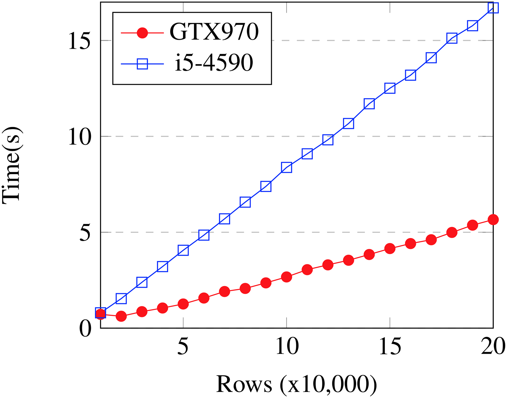
Figure 9 shows the performance of the GPU algorithm across varying problem sizes using configuration #1. The experiment is performed on subsets of the Bosch dataset using 20 boosting iterations. The GPU algorithm’s time increases linearly with respect to the number of input rows. It is approximately equal to the CPU algorithm at 10,000 rows and always faster thereafter for this dataset. This gives an idea of the minimum batch size at which the GPU algorithm begins to be effective.
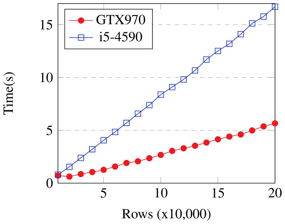
Figure 9: Bosch: time vs problem size.
In Fig. 10, we show the performance of the Titan X from configuration #2 against configuration #3 (a high-end 24 core server) on the Yahoo dataset with 500 boosting iterations and varying numbers of threads. Each data point shows the average time of eight runs. Error bars are too small to be visible at this scale. The Titan X outperforms the 24 core machine by approximately 1.2×, even if the number of threads for the 24 core machine is chosen optimally.
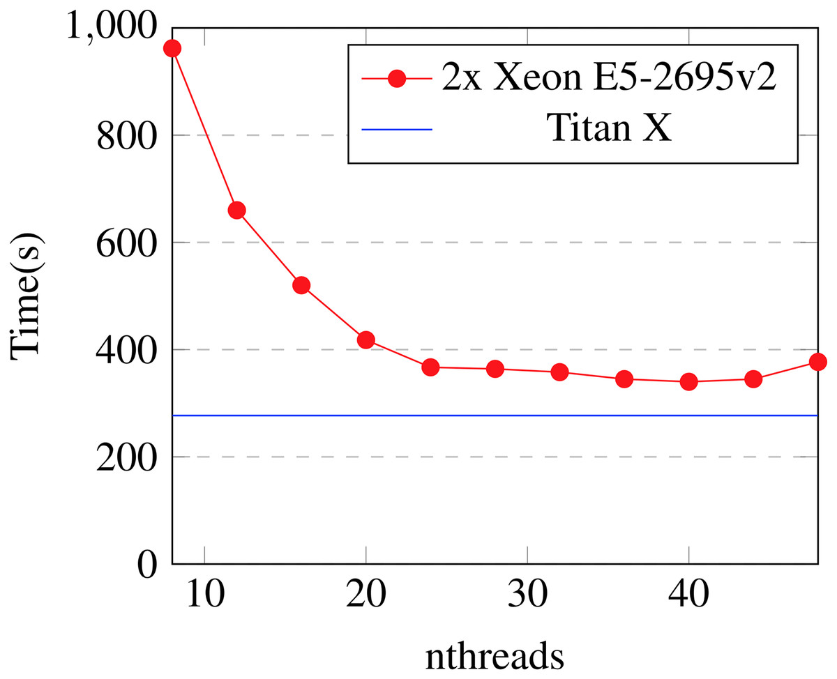
Figure 10: Yahoo LTR: n-threads vs time.
Interleaved algorithm performance
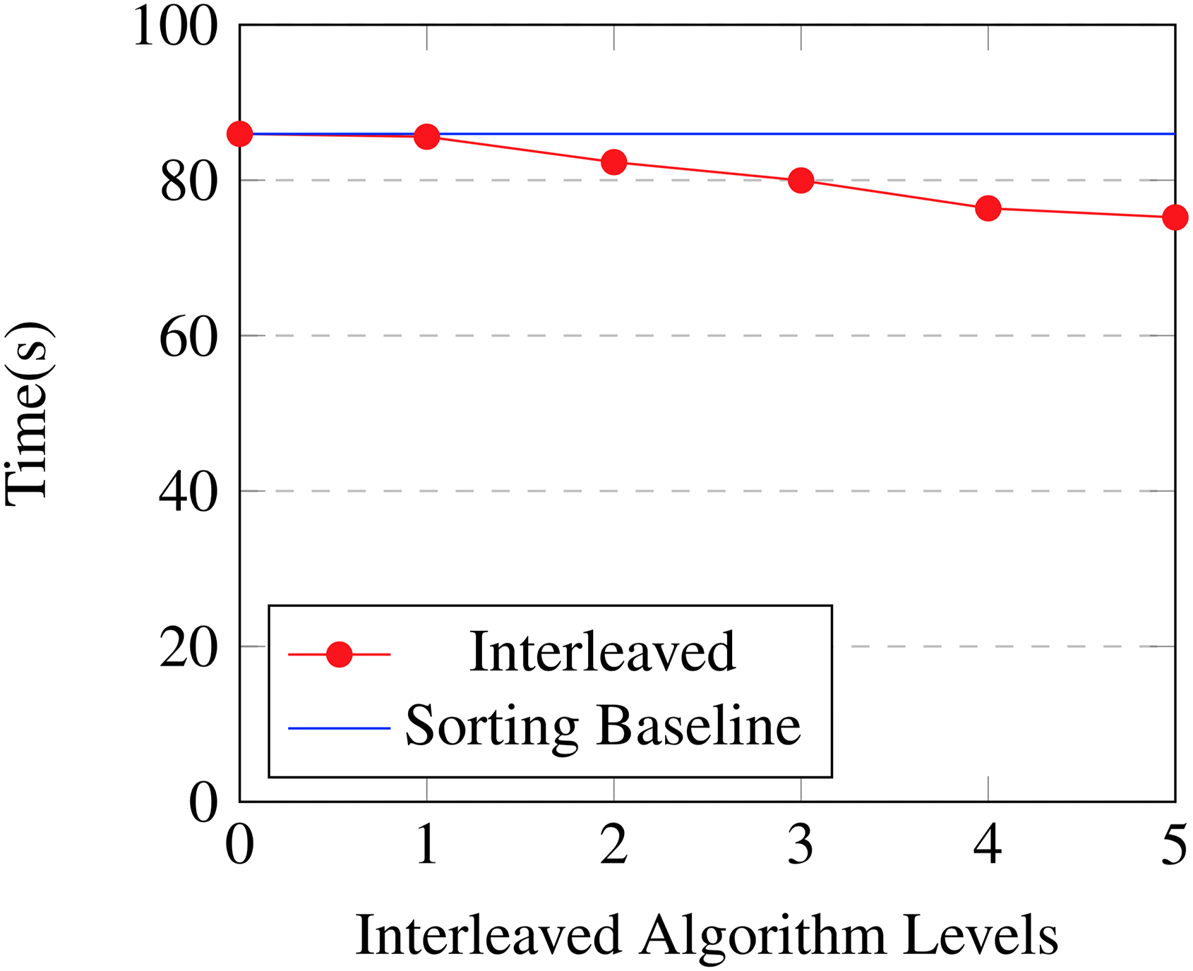
In Table 26 and Fig. 11, we show the effect of changing the threshold at which the algorithm switches between the interleaved version of the algorithm and the sorting version of the algorithm. Timings are from 100 boosting iterations on a 35% subset of the Bosch dataset using configuration #1. Using the interleaved version of the algorithm shows benefits all the way up to the fifth level with a 1.14× speed increase as compared to just using the sorting algorithm. After this depth temporary storage is insufficient to keep using the interleaved approach. Note that for the first level the interleaved algorithm and the sorting algorithm are equivalent as there is only one node bucket.
| Levels | GPU time (s) | Accuracy | Speedup |
|---|---|---|---|
| 0 | 85.96 | 0.7045 | 1.0 |
| 1 | 85.59 | 0.7102 | 1.0 |
| 2 | 82.32 | 0.7047 | 1.04 |
| 3 | 79.97 | 0.7066 | 1.07 |
| 4 | 76.38 | 0.7094 | 1.13 |
| 5 | 75.21 | 0.7046 | 1.14 |

Figure 11: Bosch: interleaved algorithm threshold.
Surprisingly the interleaved algorithm is still faster than the sorting algorithm at level 5 despite the fact that the multiscan and multireduce operations must sequentially iterate over 25 = 32 nodes at each step. This shows that executing instructions on elements held in registers or shared memory carries a very low cost relative to uncoalesced re-ordering of elements in device memory, as is performed when radix sorting.
Memory consumption
We show the device memory consumption in Table 27 for all three benchmark datasets. Each dataset can be fit entirely within the 12 GB device memory of a Titan X card. In Table 28, we show the memory consumption of the original CPU algorithm for comparison. Host memory consumption was evaluated using the valgrind massif (http://valgrind.org/docs/manual/msmanual.html) heap profiler tool. Device memory usage was recorded programmatically using custom memory allocators. The device memory requirements are approximately twice that of the original CPU algorithm. This is because the CPU algorithm is able to process data in place, whereas the GPU algorithm requires sorting functions that are not in place and must maintain separate buffers for input and output.
| Dataset | Device memory (GB) |
|---|---|
| YLTR | 4.03 |
| Higgs | 11.32 |
| Bosch | 8.28 |
| Dataset | Host memory (GB) |
|---|---|
| YLTR | 1.80 |
| Higgs | 6.55 |
| Bosch | 3.28 |
Conclusion
A highly practical GPU-accelerated tree construction algorithm is devised and evaluated within the XGBoost library. The algorithm is built on top of efficient parallel primitives and switches between two modes of operation depending on tree depth. The ‘interleaved’ mode of operation shows that multiscan and multireduce operations with a limited number of buckets can be used to avoid expensive sorting operations at tree depths below six, resulting in speed increases of 1.14× for the GPU implementation.
The GPU algorithm provides speedups of between 3× and 6× over multicore CPUs on desktop machines and a speed up of 1.2× over 2× Xeon CPUs with 24 cores. We see significant speedups for all parameters and datasets above a certain size, while providing an algorithm that is feature complete and able to handle sparse data. Potential drawbacks of the algorithm are that the entire input matrix must fit in device memory and device memory consumption is approximately twice that of the host memory used by the CPU algorithm. Despite this, we show that the algorithm is memory efficient enough to process the entire Higgs dataset containing 10 million instances and 28 features on a single 12 GB card.
Our algorithm provides a practical means for XGBoost users processing large data sets to significantly reduce processing times, showing that gradient boosting tasks are a good candidate for GPU-acceleration and are therefore no longer solely the domain of multicore CPUs.