
An ODE model of yaws elimination in Lihir Island, Papua New Guinea
- Published
- Accepted
- Received
- Academic Editor
- Martial Ndeffo
- Subject Areas
- Epidemiology, Global Health, Health Policy, Infectious Diseases, Computational Science
- Keywords
- Mathematical model, Yaws, Eradication, Morges strategy, Total community treatment, Total targeted treatment
- Copyright
- © 2022 Kimball et al.
- Licence
- This is an open access article distributed under the terms of the Creative Commons Attribution License, which permits unrestricted use, distribution, reproduction and adaptation in any medium and for any purpose provided that it is properly attributed. For attribution, the original author(s), title, publication source (PeerJ) and either DOI or URL of the article must be cited.
- Cite this article
- 2022. An ODE model of yaws elimination in Lihir Island, Papua New Guinea. PeerJ 10:e13018 https://doi.org/10.7717/peerj.13018
Abstract
Yaws is a chronic infection that affects mainly the skin, bone and cartilage and spreads mostly between children. The new approval of a medication as treatment in 2012 has revived eradication efforts and now only few known localized foci of infection remain. The World Health Organization strategy mandates an initial round of total community treatment (TCT) with single-dose azithromycin followed either by further TCT or by total targeted treatment (TTT), an active case-finding and treatment of cases and their contacts. We develop the compartmental ODE model of yaws transmission and treatment for these scenarios. We solve for disease-free and endemic equilibria and also perform the stability analysis. We calibrate the model and validate its predictions on the data from Lihir Island in Papua New Guinea. We demonstrate that TTT strategy is efficient in preventing outbreaks but, due to the presence of asymptomatic latent cases, TTT will not eliminate yaws within a reasonable time frame. To achieve the 2030 eradication target, TCT should be applied instead.
Introduction
Yaws is an infectious disease spread by skin to skin contact mostly amongst children (Marks, Solomon & Mabey, 2014). It is caused by bacteria Treponema pallidum ssp. pertenue, and begins at an abrasion or open wound which then develops into the “primary papule” or “mother yaw” (Perine et al., 1984). This initial stage is known as primary yaws and the lesion persists for three to six months (Marks et al., 2015a). A short latency period may occur after primary yaws if the primary papule naturally heals before secondary lesions develop (Perine et al., 1984). Secondary yaws begins with the appearance of other lesions anywhere on the body (Mitjà, Asiedu & Mabey, 2013). These lesions heal spontaneously resulting in a noninfectious latent period that, in some cases, may last the remaining lifetime of the person (Perine et al., 1984). During the latent period, previously infected individuals may relapse into secondary yaws up to 5 years after recovering from infection (Marks et al., 2015b). Up to 10% of yaws cases may develop into late yaws (Mitjà, Asiedu & Mabey, 2013), also known as tertiary yaws. Tertiary lesions tend to be very harmful with massive necrotic tissue destruction; yet they are noninfectious (Marks, Solomon & Mabey, 2014).
Yaws was the first disease to be targeted for eradication by the World Health Organization (Marks et al., 2015a). Before this initiative, 90 countries were reported as endemic, totaling about 50 million cases worldwide (Kazadi et al., 2014). The mass screening and treatment programmes led by WHO reduced the global prevalence by >95% between 1950 and 1964, but yaws has reemerged as a public health problem (Asiedu et al., 2008). In 2018, Papua New Guinea and the Solomon Islands reported over 10,000 suspected cases each (WHO, 2018b). According to the most recent report (WHO, 2020), 15 countries are considered as currently endemic for yaws; 87,877 suspected yaws cases were reported to WHO in 2020 from 11 countries from which 81,369 cases were in Papua New Guinea. Solomon Islands reported 13,694 cases in 2019. Figure 1 shows the most recent status of yaws endemicity.
A single oral dose of azithromycin was shown to be just as effective as the previous treatment of injectable penicillin (Mitjà et al., 2012). This initiated a new wave of interest in eradication of yaws (Marks et al., 2015a) and, in 2012, the WHO implemented the Morges Strategy to combat yaws transmission with the goal of eradicating the disease by 2020 (WHO, 2012). The Morges Strategy includes one or more rounds of total community treatment (TCT) where treatment is given to all members of the community and followed by the total targeted treatment(TTT) where treatment is administered to all actively infected individuals and their close contacts as a response to a local outbreak (WHO, 2012). This strategy continues to be the primary plan to eradicate yaws, but the timeline has been stretched to eradication by 2030 after the original 2020 goal was not met (Dyson et al., 2019).
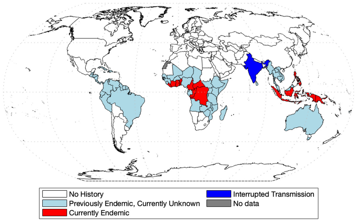
Figure 1: World map of endemic history and prevalence of yaws.
Data collected from WHO (2018b) and WHO (2020) and map was made with the aid of borders.m file (Greene et al., 2019) in MATLAB.
Mathematical modelling is now a standard and indispensable tool for understanding disease dynamics and control (Anderson & May, 1992), yet there is a surprising lack of models of yaws transmission. Until 2012, the only math model of yaws considered the effect of the chicken pox virus on yaws (Gart & De Vries, 1966). More recently, the model from Mushayabasa et al. (2012) divides the population into rich and poor and preforms a theoretical analysis of disease-free and endemic equilibria. In Muench (2013), the authors fitted a simple catalytic model to age structured yaws data. All other models of yaws are stochastic and were designed to estimate various aspects of yaws eradication. In Fitzpatrick, Asiedu & Jannin (2014), the authors were concerned with the economic side of eradication and concluded that the eradication would not be expensive; yet there is still a large degree of uncertainty for the lack of available data (Dyson et al., 2019). In Dyson et al. (2017), the authors created a model to estimate the fraction of individuals that are missed during treatment in the Morges strategy. In modeling effectiveness of the Morges Strategy, Marks et al. (2017) investigated the probability of eradication. Fitzpatrick et al. (2018) created a linear regression model in order to predict the probability of case reporting in different previously affected countries based on different parameters. Mooring et al. (2019) builds off of the work of Marks et al. (2017), using the same compartment model and modeling the effects of different combinations of TTT and TCT. The most recent model comes from Holmes et al. (2020) in which the authors adapted the model from Dyson et al. (2017) to again simulate different combinations of TTT and TCT. It was found that different populations require different treatments, but in general, TCT was more effective in eradication.
The stochastic models such as recent Marks et al. (2017); Mooring et al. (2019); Holmes et al. (2020) are generally more suitable for the eradication end game than the deterministic compartmental models. Yet, the deterministic models are typically simple and easy to analyze, while still reasonably accurate and realistic. Given the lack of deterministic models of yaws transmission in general, our goal is to develop a deterministic model of yaws transmission and then use the model to compare the effectiveness of TTT and TCT strategies. We use the model to derive a formula for the basic reproduction number and to obtain simulated times needed for yaws elimination. Our model can be used as a quick estimate of the effectiveness of a particular treatment strategy.
Methods
We created a compartmental model shown in Fig. 2. Individuals are born as susceptible (S) at rate Λ. The susceptible individuals become exposed (E) after coming in contact with individuals having primary (Y1) or secondary (Y2) yaws; the transmission rate is β. After an incubation period lasting a time σ−1, the exposed individual develops primary yaws and becomes infectious. The primary yaws lasts a time , after which the individual may either develop secondary yaws (Y2) with probability pY1Y2, or go into a first latency period (L1) with probability pY1L1 = 1 − pY1Y2. This means that the rate of progression from Y1 to L1 is pY1L1λ1 while the rate of progression from Y1 to Y2 is pY1Y2λ1.

Figure 2: Scheme of the yaws dynamics.
The arrows denote transitions between the compartments. The letters next to the arrows specify the per capita rates of the transitions. The red arrows denote a treatment. The black arrows show a natural disease progression (without any treatment), from susceptible (S) to exposed (E) and then to primary yaws (Y1). After the primary yaws, a majority of cases goes through a short latent period (L1) before progressing to secondary yaws (Y2). A small portion develops secondary yaws directly. Most secondary yaws heals and the infection becomes latent (L2). The latent cases can relapse to secondary yaws for the rest of their lives. Only a negligible number of individuals develop non-infectious tertiary yaws (Y3).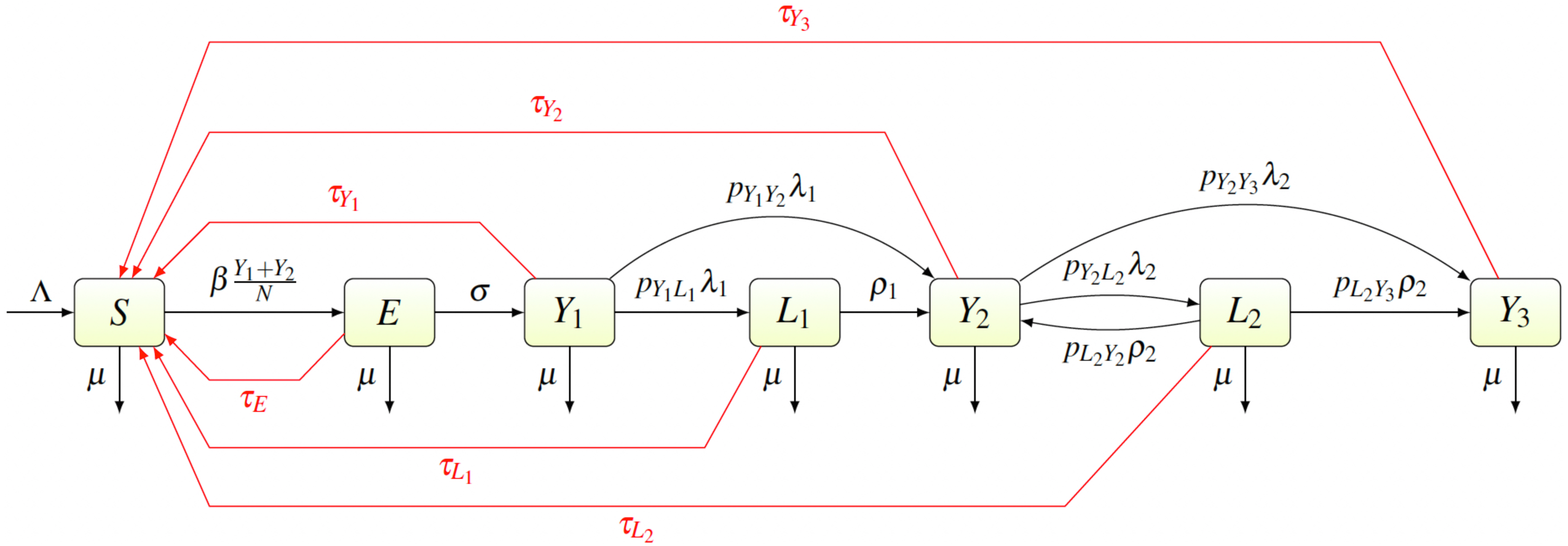
The average duration of the first latency period is ; after that an individual develops secondary yaws. The average duration of secondary yaws is . After this period, one could either develop rare, debilitating and very painful, but non-infectious, tertiary yaws (Y3) with probability pY2Y3, or go into the second latent period with probability pY2L2 = 1 − pY2Y3. The average length of the second latency period is . Afterwards, individuals can relapse into secondary yaws with a probability pL2Y2, or develop tertiary yaws with a probability pL2Y3 = 1 − pL2Y2.
Individuals can be treated and return to susceptible at a rate of τI for individuals in a compartment I ∈ {E, Y1, Y2, Y3, L1, L2}. Treatment of each compartment depends on the elimination strategy and the specific values are discussed below.
Finally, all individuals are assumed to die at rate µ.
The parameters are summarized in Table 1. Most parameter values were estimated directly from the literature. The only two exceptions are the transmission rate β and the treatment rates τ. Details are shown in Appendix B.
| Symbol | Meaning | Value | Range | Source |
|---|---|---|---|---|
| Λ | Birth rate | [0.001, 0.003] | United Nations (2019) | |
| μ−1 | Expected life span | 65∗12 | [600, 1200] | World Bank (2019) |
| β | Transmission rate | 0.0166 | [0.01, 0.02] | Estimated |
| σ−1 | Length of the incubation period | Perine et al. (1984) | ||
| λ1−1 | Length of primary yaws | 3 | [3, 6] | Perine et al. (1984) |
| λ2−1 | Length of secondary yaws | 3 | [0, 60] | Mitjà, Asiedu & Mabey (2013) |
| ρ1−1 | Length of latency after primary yaws | 1.5 | [1, 2] | Marks et al. (2015a) |
| ρ2−1 | Length of second latency | 30 | [1, 60] | Perine et al. (1984) |
| pY1Y2 | Probability of immediate secondary yaws infection after primary yaws | 0.12 | [0.09, 0.15] | Mitjà, Asiedu & Mabey (2013) |
| pY1L1 | Probability of latency period after primary yaws | 1 − pY1Y2 | ||
| pY2Y3 | Probability of immediate tertiary yaws infection after secondary yaws | 0.0001 | [0, 0.0002] | Mitjà, Asiedu & Mabey (2013) |
| pY2L2 | Probability of latency period after secondary yaws | 1 − pY2Y3 | ||
| pL2Y2 | Probability of relapsing to secondary yaws during latent period after secondary yaws | 0.9999 | [0.9998, 1] | Mitjà, Asiedu & Mabey (2013) |
| pL2Y3 | Probability of developing tertiary yaws during latent period | 1 − pL2Y2 | ||
| τI | Rate of treatment for the group I ∈ {E, Y1, Y2, Y3, L1, L2} | variable | See text |
The transmission rate β was obtained by fitting the endemic equilibrium to baseline data (prior the mass treatment, i.e., when all τI = 0) from Lihir Island in Papua New Guinea (Mitjà et al., 2015b).
To model TCT, we assume τI = 1/6 for all I, corresponding to treating the whole population every six months. To model TTT, we assume the best case scenario, i.e., τE = τY1 = τY2 = τY3 = τL1 = 1/6 while τL2 = 0.1/6, i.e., we assume that the TTT strategy finds and treats only 10% of secondary latent cases every six months but otherwise finds and treat every other infected individual. This again corresponds to treating active yaws cases and all their closed contacts (that will be either exposed or at most the first latency period) once in six months. We assume that 90% of secondary latent cases are omitted in the treatment because the were infected independently many months or even years ago and are not close contacts to the currently acutely infected individuals. We adopted these assumptions since we can then demonstrate that even these high coverage, yaws will persist in the population for long time under TTT strategy. The protocol of Mitjà et al. (2015b) study also included a 2 year period of non-strategic treatment. For that period, we assumed τE = τY1 = τY2 = τY3 = τL1 = 1/24 with coverage as in TTT.
We validated our model on data from the mass treatment trial in Lihir Island (Mitjà et al., 2018); see Fig. 3. The fitted curve follows general trends of the data. However, the real data for latent infections exhibits oscillation with peaks and dips every 6 months and our simple model cannot exhibit such oscillations.
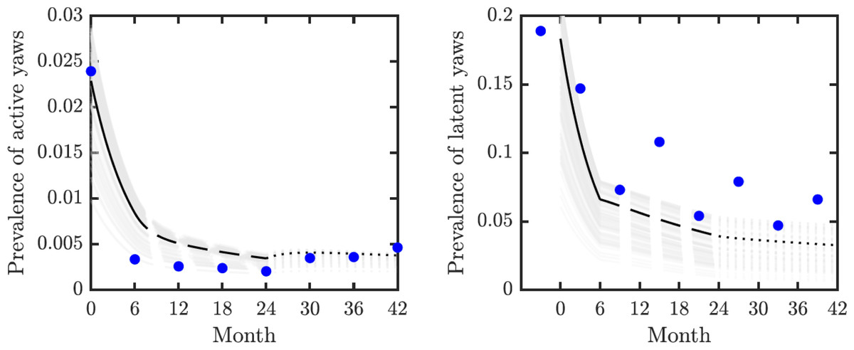
Figure 3: Model validation.
Data from Mitjà et al. (2018) (blue circles) track active (left) and latent (right) yaws prevalence on Lihir Island. The study protocol was one round of TCT at time 0, followed by three rounds of TTT every six months till month 24 and then non-strategic treatment till month 42 (Mitjà et al., 2015b). The latent cases data (right) are plotted 3 months earlier to account for the continued seropositivity of latent infections until 3–6 months after treatment (Mitjà et al., 2012). The model predictions show one round of TCT (solid line, months 0–6) followed by TTT (dashed line, months 6–24) and then a period of non-strategic treatment (dotted line, during months 24–42). The black lines represent the model predictions for the parameters as in Table 1. The gray lines represent model predictions when the parameters value vary within the ranges specified in Table 1.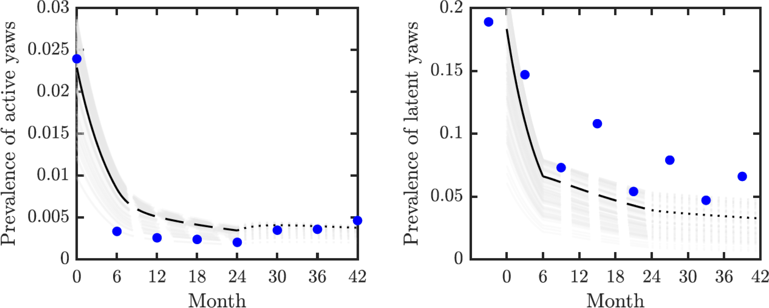
We used the compartmental model from Fig. 2 to create a system of ordinary differential equations. We found disease-free and endemic equilibria. Using the next generation matrix method (van den Driessche & Watmough, 2002), we found the basic reproduction number. We performed the stability analysis of the disease-free equilibria based on methods from van den Driessche & Watmough (2002) and Castillo-Chavez et al. (2002).
We did simulations in MATLAB, the code is made available in supplementary material. We adhered to responsible coding practices as outlined in Lucas et al. (2020).
The global uncertainty and sensitivity analysis by the partial rank correlation coefficients, PRCC was based on Marino et al. (2008). We randomly selected 1000 parameter values within the ranges specified in Table 1. We used only those values that could fit to baseline data from Lihir Island (Mitjà et al., 2015b).
Results
We obtained an explicit formula for the basic reproduction number, R0. As shown in Eq. (9), (1) where vI denote the sum of all total rates out of the compartment I, i.e., (2) (3) (4) (5) (6) (7) We estimated that without any treatment, R0 = 1.2548. The uncertainty analysis showed that in order to fit data from Lihir Island, R0 is between 1.24 and 1.27; see Fig. 4. With TTT treatment, the values of R0 ranged between 0.02 and 0.08. This shows that TTT is quite effective in prevention of the spreading of the epidemics.
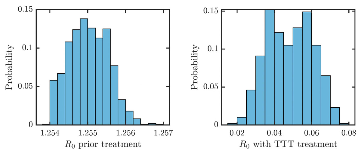
Figure 4: Distribution of R0 for parameters that fit data from Lihir Island (Mitjà et al., 2015b).
Left: Prior the treatment. Right: during TTT treatment.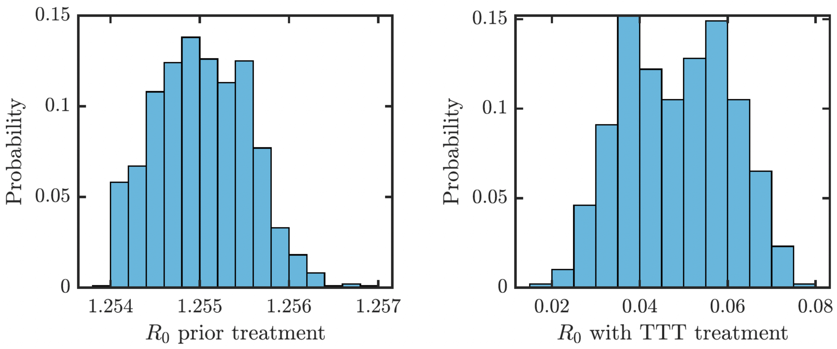
We proved (Theorem 1 in Appendix A.2) that the disease-free equilibrium is globally asymptotically stable when the basic reproduction number R0 < 1. We also showed (Lemma 1 in Appendix A.2) that R0 is decreasing in the treatment rate. If the treatment rate is high enough, the basic reproduction number drops below 1 even for a conservative TTT strategy when only active cases of yaws gets treated; see Fig. 5. This means that the Morges strategy can eventually eliminate yaws.
Figure 5: Dependence of R0 on τ under TCT and TTT regimes.
Once τ > τ0 where τ0 solves R0 = 1, then the disease can be eliminated. For the parameters as in Table 1, τ0,TCT ≈ 3.5⋅10−4 and τ0,TTT ≈ 1.68⋅10−3.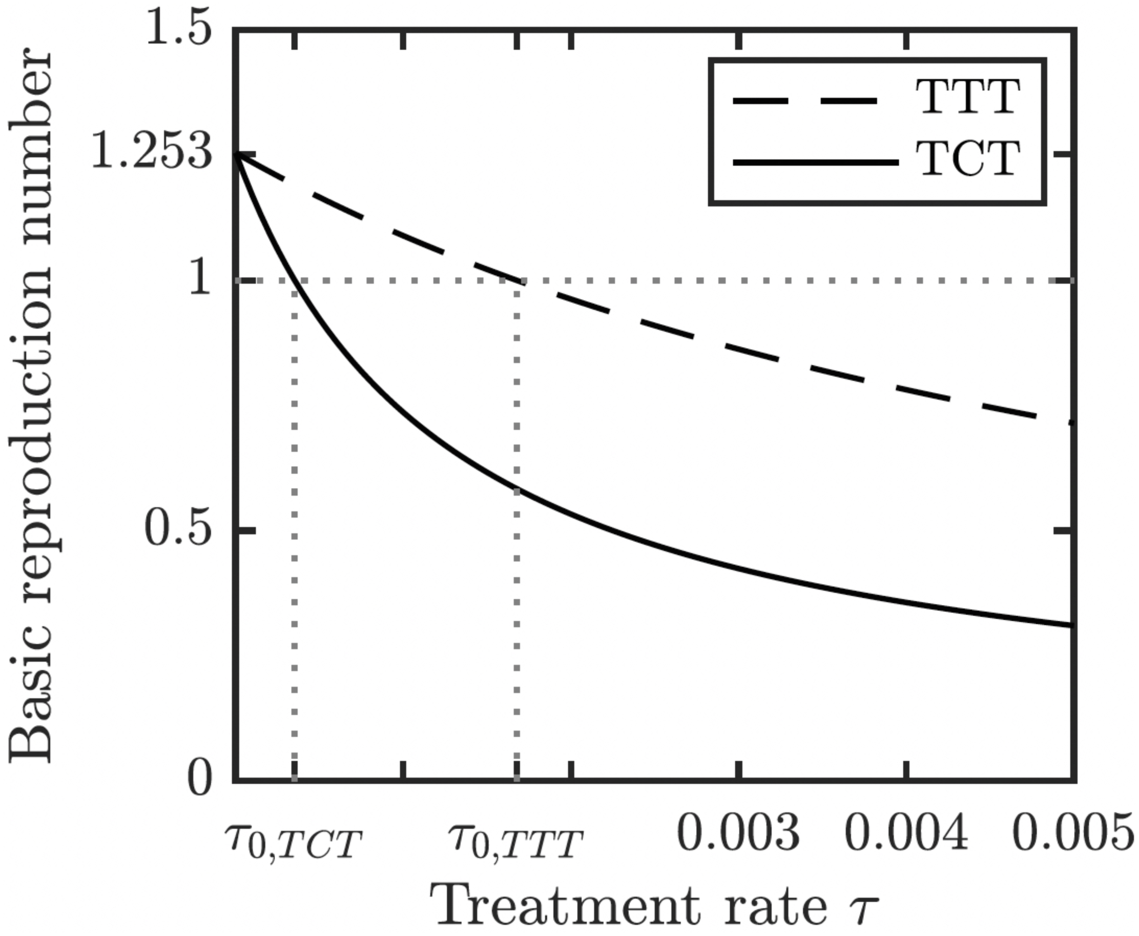
To understand how long the Morges strategy needs to be applied, we simulated two rounds of initial TCT and followed by subsequent rounds of TTT. We performed a global uncertainty analysis where we varied parameters within the ranges specified in Table 1. Figure 6 demonstrates the results. Our model predicts that it would take about 14 to 16 years to achieve a thousandfold decrease in cases (i.e., less than 1 infected person in Lihir Island). The relatively high prevalence of latent cases in the population and the long latency period are the main culprits behind this long elimination time. The continuous application of TCT strategy every six months can achieve the same results in about 3.5 years; the improvement in speed is caused by the latent cases getting treated as well.
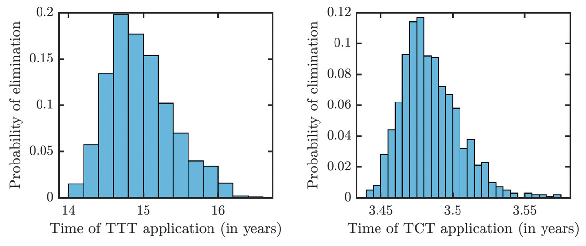
Figure 6: Distribution of times needed to decrease yaws cases thousand times using TTT (left) or TCT (right).
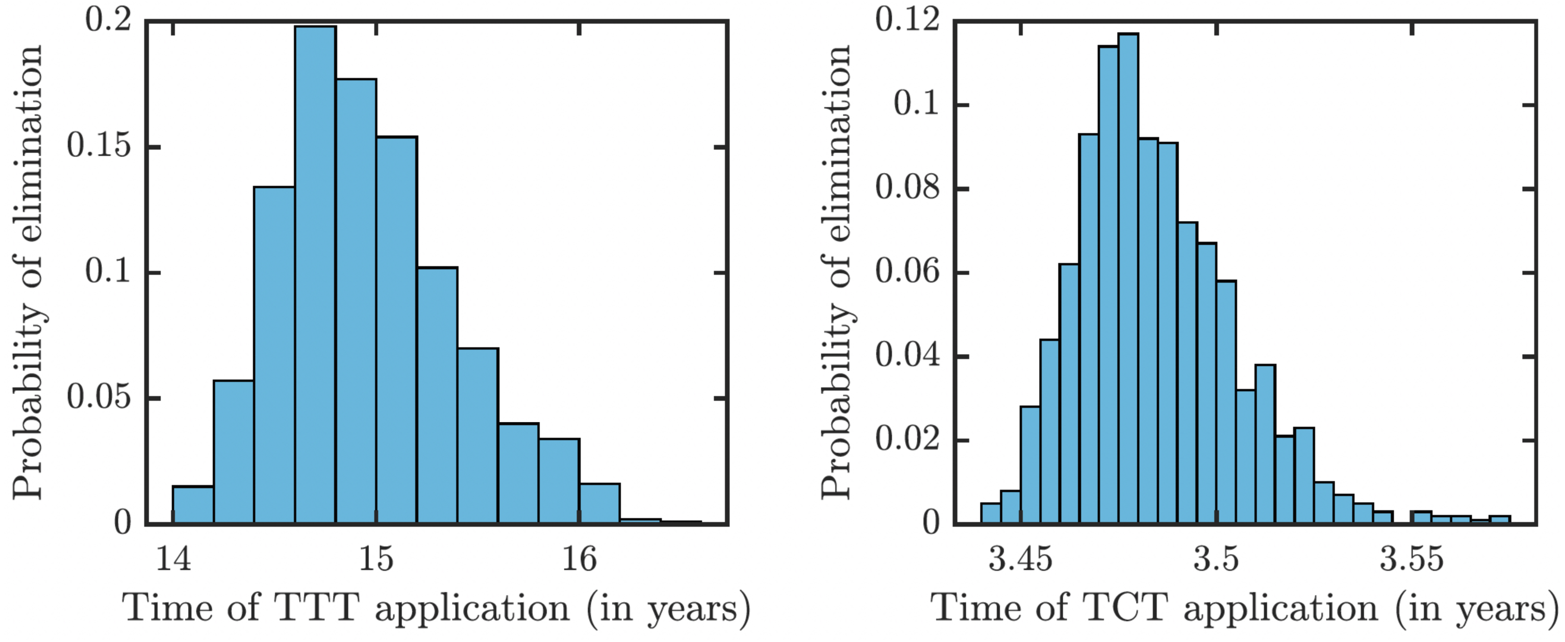
As illustrated in Fig. 7, the success or failure of TTT strategy significantly depends on how many latently infected individuals can be discovered and treated. The figure in fact shows expected elimination times for a whole family of strategies with TTT on one end (when the coverage of L2 is low) and TCT on the other end (when the coverage of L2 is 100%). It can take over 25 years to eliminate yaws if only 1% or less of latent cases are found; it would take about about 10 years if 20% is found and about 5 years if about 50% of cases is found.
Figure 7: Sensitivity analysis of the time needed to eliminate yaws under TTT.
We showed the dependence on the percentage of treated L2 cases explicitly. The analysis of other parameters is done by partial rank correlation coefficients, PRCC (Marino et al., 2008).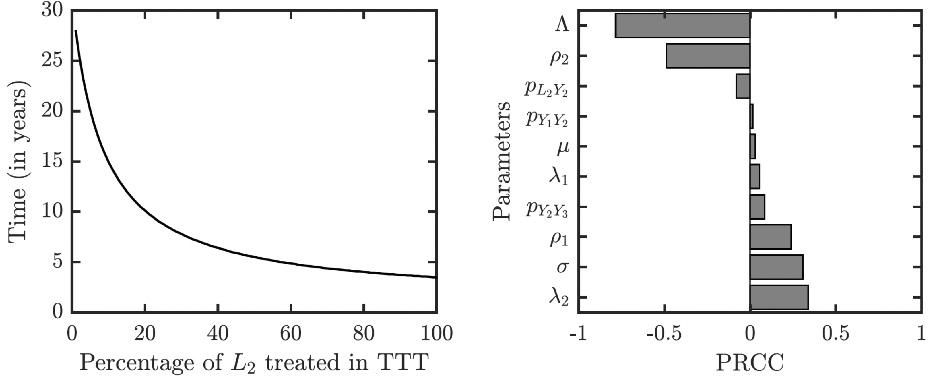
The sensitivity analysis shows a strong influence of the relapse rate, ρ2, and the spontaneous healing rate of the secondary yaws, λ2, on the elimination time under the TTT regime; see Fig. 7. The higher the relapse rate and the lower the healing rate, the less it takes to eliminate yaws. This initially counter-intuitive result is caused by the fact that spontaneous healing increases the pool of latently infected individuals that can be missed by the TTT strategy. However, if infected individuals do not heal spontaneously, they can be discovered and treated. This again indicates that the latent individuals are the weakest point of the TTT strategy. A higher birth rate also reduces the time to elimination. This is mainly because a higher birth rate increases the influx of healthy individuals while the active yaws of young children are caught on time before progressing to latency. Naturally, a shorter incubation periods increases the time needed for the elimination as they increase the number of yaws cases. The effects of other parameters are relatively mild and not significant.
Finally, let us note that when R0 > 1, the disease-free equilibrium is not stable and there exists an endemic equilibrium given explicitly in Eq. (10). We run numerical simulations for parameter values with ranges in Table 1 and the numerical solutions of the ODE model always converged to the endemic equilibrium. Moreover, motivated by Yang et al. (2017) and LaSalle (1976), we considered a Lyapunov function , where the summation is taken over all compartments C ∈ {S, E, Y1, Y2, Y3, L1, L2} and C∗ is an endemic equilibrium value. It follows that and iff C = C∗ for all compartments. Also, we evaluated at 105 randomly selected values of the compartments. We always saw that . Thus, we believe that the endemic equilibrium is globally stable whenever R > 1, although we do not have an analytical proof of this fact. However, as it has been shown in Fig. 4, even with the weaker TTT treatment, R0 is significantly less than 1 and thus, for the purpose of the elimination (which is the main focus of this paper), the stability of the disease-free equilibrium is much more important.
Discussion
To model TTT strategy, we made a conservative assumption that not many latent cases are treated. We argue that this is a reasonable reflection of a reality in the eradication endgame. The latent cases represent reservoir of future infections Dyson et al. (2019). By treating a recently relapsed latent case with all its close contacts, TTT strategy prevents outbreaks. However, contact tracing does not identify many other latent cases in the population; they likely got infected independently many months or even years ago. Thus, TTT works quite slowly as an elimination strategy as it is equivalent to waiting for the latent cases to relapse instead of actively identifying and treating them while still asymptomatic.
Our model predicts very little variation of eradication times when using TCT strategy. This is natural as the whole population gets treated and most factors of yaws dynamics thus do not play any crucial role. The variability is much larger for the TTT regime which could potentially eliminate yaws in as little as 14 years but it may also take 16 years. The two key factors responsible for the large variation are the duration of the latent period (which is positively correlated with the elimination time) and the duration of the secondary yaws (which is negatively correlated with the elimination times). Gaining more knowledge about these two parameters would reduce the uncertainty of the model predictions.
Our model differs from previous models in two crucial aspects. First, we developed a deterministic ODE model, in contrast to recent stochastic models developed in Fitzpatrick, Asiedu & Jannin (2014); Marks et al. (2017); Dyson et al. (2017); Fitzpatrick et al. (2018); Holmes et al. (2020). While stochastic simulations can incorporate higher degrees of realism, there is a natural simplicity in the ODE models that allows for an easy estimation of the basic reproduction number. Even with different model parameters, we do not necessarily have to rerun the simulations to be able to predict the model outcomes. Our model can thus serve as a first and reasonably reliable estimate of what will happen under different elimination strategies.
Second, our model incorporates all of the known stages of yaws. All models of yaws should consider susceptible individuals, infectious stage(s) of yaws (possibly divided into primary and secondary yaws) and the asymptomatic latent yaws that can relapse. Similarly to Fitzpatrick, Asiedu & Jannin (2014), we also considered tertiary yaws; and as Mushayabasa et al. (2012), we included exposed individuals. Finally, as in Marks et al. (2017) we included a possibility of a latent period between the primary and secondary yaws.
There are several limitation of our model. Most of the limitations stem from the fact that our model is a simple deterministic ODE model in homogeneous population. It thus cannot capture the true eradication endgame when only very small, often just a single digit, number of individuals are infected. The model also cannot capture household dynamics as done in Dyson et al. (2017) or the population structured into hamlets as done in Mooring et al. (2019).
Unlike in stochastic simulations used in Marks et al. (2017); Dyson et al. (2017); Mooring et al. (2019); Holmes et al. (2020), we do not explicitly consider treatment coverage. An independent coverage is implicitly incorporated in our model—a rate τI = 1/6 can mean that the whole (100%) population is treated once every 6 months, as well as that the attempt to treat the whole population is made every m months but at each attempt, only p∗100% of the population is reached with m/p = 6. A systematic failure of the treatment could be included in the model by duplicating each compartment into “treatment adherent“ and “treatment non-adherent”. Setting the birth rate as (1 − p)Λ and pΛ, respectively, into the susceptible treatment adherent and treatment non-adherent, respectively, would then achieve a systematic failure of treatment for p∗100% of the population.
Economics plays a key role in the feasibility of yaws eradication. Our model should be extended by explicitly optimizing control strategies, i.e., the proper combination of TCT and TTT at the appropriate time intervals. The extensions need to take into the account that underdeveloped areas are more prone to transmission and are harder to screen for active infections.
Conclusions
Our paper is the first ODE compartment model specifically applied to yaws elimination. We investigated two strategies, the total community treatment (TCT) and the total targeted treatment (TTT). In agreement with previous models (Dyson et al., 2017; Marks et al., 2015c), we found that due to the high prevalence of latent infections, it is very hard to eliminates yaws by using TTT. Our model predicts that it would take about 15 years to reduce the prevalence thousandfold from the current levels. On the other hand, it would take only about 3.5 years if the whole community was treated once every six months. This is in a quantitative agreement with a recent detailed stochastic model (Holmes et al., 2020). We also note that due to the global stability of the disease-free equilibrium, and the fact that R0 is significantly less than 1 even under TTT treatment, the initial levels of yaws in the population do not play a crucial role for the eradication.
In the light of above findings, we thus recommend using total community treatment as the primary yaws elimination strategy. This recommendation is further supported by the fact that (a) TCT provides additional benefits such as reduction in trachoma prevalence (Solomon et al., 2015), (b) the cost of TCT is not much larger that the cost of TTT (Fitzpatrick, Asiedu & Jannin, 2014), and (c) TTT requires active surveillance (Fitzpatrick et al., 2018), possibly further erasing the difference between the costs of these two approaches. As a note of caution, our model did not consider emergence of antibiotic resistant strains (Mitjà et al., 2018). It is a question whether a large scale application of TCT could eliminate yaws before the antibiotic resistance becomes a true obstacle.