
A new optimization algorithm based on mimicking the voting process for leader selection
- Published
- Accepted
- Received
- Academic Editor
- Bilal Alatas
- Subject Areas
- Algorithms and Analysis of Algorithms, Artificial Intelligence, Data Science, Optimization Theory and Computation
- Keywords
- Optimization, Optimization problem, Human-based metahurestic algorithm, Stochastic algorithms, Population-based algorithms, Applied mathematics, Voting process, Leader selection, Population matrix, Recurring process
- Copyright
- © 2022 Trojovský and Dehghani
- Licence
- This is an open access article distributed under the terms of the Creative Commons Attribution License, which permits unrestricted use, distribution, reproduction and adaptation in any medium and for any purpose provided that it is properly attributed. For attribution, the original author(s), title, publication source (PeerJ Computer Science) and either DOI or URL of the article must be cited.
- Cite this article
- 2022. A new optimization algorithm based on mimicking the voting process for leader selection. PeerJ Computer Science 8:e976 https://doi.org/10.7717/peerj-cs.976
Abstract
Stochastic-based optimization algorithms are effective approaches to addressing optimization challenges. In this article, a new optimization algorithm called the Election-Based Optimization Algorithm (EBOA) was developed that mimics the voting process to select the leader. The fundamental inspiration of EBOA was the voting process, the selection of the leader, and the impact of the public awareness level on the selection of the leader. The EBOA population is guided by the search space under the guidance of the elected leader. EBOA’s process is mathematically modeled in two phases: exploration and exploitation. The efficiency of EBOA has been investigated in solving thirty-three objective functions of a variety of unimodal, high-dimensional multimodal, fixed-dimensional multimodal, and CEC 2019 types. The implementation results of the EBOA on the objective functions show its high exploration ability in global search, its exploitation ability in local search, as well as the ability to strike the proper balance between global search and local search, which has led to the effective efficiency of the proposed EBOA approach in optimizing and providing appropriate solutions. Our analysis shows that EBOA provides an appropriate balance between exploration and exploitation and, therefore, has better and more competitive performance than the ten other algorithms to which it was compared.
Introduction
Optimization is an integral part of engineering, industry, technology, mathematics, and many other applications in science. Decision variables, constraints, and objective function are the three main parts of any optimization issue, where determining the values of decision variables while respecting the constraints to optimize the objective function is the main challenge of optimization (Ray & Liew, 2003).
Optimization problem solving approaches are included in two groups: deterministic and stochastic (Kozlov, Samsonov & Samsonova, 2016). Deterministic approaches, which include gradient-based and non-gradient-based techniques, have successful performance in handling convex and linear optimization problems. However, these approaches fail to meet real-world challenges with features such as convex behavior, nonlinear search space, high number of variables, complex objective function, high number of constraints, as well as NP-hard problems. Following the inability of deterministic approaches to address these types of issues, researchers have developed a new approach called stochastic optimization techniques. Metaheuristic algorithms are one of the most widely used stochastic approach techniques that are effective in optimization applications by using random operators, random scanning in the search space, and trial and error (Curtis & Robinson, 2019).
Simplicity of concept, ease of implementation, problem-independent, needlessness of the derivation process, and efficiency in complex problems are some of the advantages that have led to the popularity and applicability of metaheuristic algorithms (Gonzalez et al., 2022).
Metaheuristic algorithms have a nearly identical problem-solving process that begins with the production of a certain number of candidate solutions at random. Then, in a repetition-based process, the effect of the algorithm steps on these candidate solutions improves them. At the end of the implementation, the best-founded candidate solution is introduced as the solution to the problem (Toloueiashtian, Golsorkhtabaramiri & Rad, 2022).
It is important to note here that there is no guarantee that metaheuristic algorithms will be able to provide the best optimal solution known as the global optimal. This is due to the random nature of the search process of these algorithms. For this reason, the solution obtained from metaheuristic algorithms is called quasi-optimal (Yu, Semeraro & Matta, 2018).
The two indicators of exploration with the concept of global search and exploitation with the concept of local search are effective in the performance of metaheuristic algorithms in handling optimization problems and providing better quasi-optimal solutions (Mejahed & Elshrkawey, 2022). What has led researchers to develop numerous optimization methods is to achieve better solutions closer to the global optimal.
The main research question is whether there is a need to develop new metaheuristic algorithms given that countless algorithms have been developed so far. This question is answered with the concept of the No Free Lunch (NFL) theorem (Wolpert & Macready, 1997). The NFL theorem explains that the effective performance of an algorithm in solving a set of optimization problems does not create any presuppositions on the ability of that algorithm to provide similar performance in other optimization applications. In other words, it cannot be claimed that a particular metaheuristic algorithm performs best in the face of all optimization problems compared to all other optimization methods. The NFL theorem is the main incentive for the authors to design new optimization approaches that perform more effectively in solving optimization problems in a variety of applications. The NFL theorem has motivated the authors of this article to develop a new metaheuristic algorithm applicable in optimization challenges that is effective in providing solutions closer to the global optimization.
The novelty of this article is in introducing and designing a new metaheuristic algorithm named Election-Based Optimization Algorithm (EBOA), which its fundamental inspiration is the simulation of the voting process and the popular movement. The main contributions of this study are as follows:
-
A novel human-based Election-Based Optimization Algorithm (EBOA) is proposed.
-
The process of public movement and the electoral voting process are examined and then mathematically modeled in the EBOA design.
-
The efficiency of EBOA in optimizing thirty-three objective functions (i.e., unimodal, high-dimensional multimodal, and fixed-dimensional multimodal, and CEC 2019) is tested.
-
The quality of EBOA results is compared with ten state-of-the-art metaheuristic algorithms.
The rest of the article is structured in such a way that the literature review is presented in ‘Lecture Review’. Then in ‘Election-Based Optimization Algorithm’ the proposed EBOA is introduced and modeled. Simulation studies are presented in ‘Results’. The discussion is provided in ‘Discussion’. Conclusions and several research directions for future studies are presented in ‘Conclusions’.
Lecture review
Natural phenomena, the behavior of living things in nature, the biological sciences, genetic sciences, the laws of physics, the rules of the game, human behavior, and any evolutionary process that has an optimization process have been the source of inspiration in the design and development of metaheuristic algorithms. Accordingly, metaheuristic algorithms fall into nine groups: swarm-based, biology-based, physics-based, human-based, sport-based, math-based, chemistry-based, music-based, and the other hybrid approaches (Akyol & Alatas, 2017).
Behaviors of living organisms such as animals, birds, and insects have been the main source of ideas in the development of numerous swarm-based algorithms. The most common feature used in many swarm-based methods is the ability of living organisms to search for food sources. The most popular methods developed based on food search process modeling are the Particle Swarm Optimization (PSO) based on the search behavior of birds and fish (Kennedy & Eberhart, 1995), Ant Colony Optimization (ACO) based on ants search for the shortest path to food (Dorigo, Maniezzo & Colorni, 1996), Artificial Bee Colony (ABC) based on bee colony search behavior (Karaboga & Basturk, 2007), the Butterfly Optimization Algorithm (BOA) based on search and mating behavior of butterflies (Arora & Singh, 2019), and the Tunicate Search Algorithm (TSA) based on search behavior tonics (Kaur et al., 2020). The process of reproduction among bees and the scout bees search mechanism to find suitable new places for hives have been employed in the designing Fitness Dependent Optimizer (FDO) (Abdullah & Ahmed, 2019). Chimpanzee’s hunting strategy using operators such as emotional intelligence and sexual motivation has been the main source of inspiration in designing the Chimp Optimization Algorithm (ChOA) (Khishe & Mosavi, 2020).
Modeling of hunting strategies of living organisms in the wild has been a source of inspiration in designing various optimization approaches, including Grey Wolf Optimizer (GWO) based on gray wolf strategy (Mirjalili, Mirjalili & Lewis, 2014), Whale Optimization Algorithm (WOA) (Mirjalili & Lewis, 2016) based on humpback whales strategy, and Pelican Optimization Algorithm (POA) based on pelican behavior (Trojovský & Dehghani, 2022).
Applying the concepts of biology, genetics, and natural selection alongside random operators such as selection, crossover, and mutation has led to the development of biology-based algorithms. The process of reproduction, Darwin’s evolutionary theory, and natural selection are key concepts in the development of two widely used methods, the Genetic Algorithm (GA) (Goldberg & Holland, 1988) and the Differential Evolution (DE) algorithm (Storn & Price, 1997). The mechanism of the immune system in the face of diseases, viruses, and microbes has been the major inspiration in the development of the artificial immune system (AIS) method (Hofmeyr & Forrest, 2000).
Many phenomena, laws, and forces in physics science have been employed as inspiration sources for the development of physics-based metaheuristic algorithms. The phenomenon of melting and cooling of metals, which is known in physics as the refrigeration process, has been the main inspiration in the development of the Simulated Annealing (SA) approach (Van Laarhoven & Aarts, 1987). The phenomenon of the water cycle based on its physical changes in nature has inspired the Water Cycle Algorithm (WCA) (Eskandar et al., 2012). Gravitational force and Newton’s laws of motion have been the main concepts employed to introduce the method of Gravitational Search Algorithm (GSA) (Rashedi, Nezamabadi-Pour & Saryazdi, 2009). The application of Hook’s law and spring tensile force has been the main inspiration in Spring Search Algorithm (SSA) design (Dehghani et al., 2020a). Various physical theories and concepts have been the source of inspiration in the development of physics-based methods such as Multiverse Optimizer (MVO), inspired from cosmology concepts (Mirjalili, Mirjalili & Hatamlou, 2016), Big Bang-Big Crunch (BB-BC) inspired from Big Bang and Big Crunch theories (Erol & Eksin, 2006), Big Crunch Algorithm (BCA) inspired from Closed Universe theory (Kaveh & Talatahari, 2009), Integrated Radiation Algorithm (IRA) inspired from gravitational radiation concept in Einstein’s theory of general relativity (Chuang & Jiang, 2007), and Momentum Search Algorithm (MSA) inspired from momentum concept (Dehghani & Samet, 2020).
Behavior, thought, interactions, and collaborations in humans have been designed ideas in the development of human-based approaches. The most widely used human-based method is the Teaching-Learning-Based Optimization (TLBO) algorithm, which mimics the classroom learning environment and the interactions between students and teachers (Rao, Savsani & Vakharia, 2011). The competition between political parties and the efforts of parties to seize control of parliament is the source of inspiration in designing the Parliamentary Optimization Algorithm (POA) (Borji & Hamidi, 2009). The economic activities of the rich and the poor to gain wealth in society have been the main inspiration for the Poor and Rich Optimization (PRO) approach (Moosavi & Bardsiri, 2019). Influencing people in the community from the best successful people in the community has been the main idea of the Following Optimization Algorithm (FOA) (Dehghani, Mardaneh & Malik, 2020). The mechanism of admission of high school graduates to the university and the process of improving the educational level of students has been the main idea in designing the Learner Performance-based Behavior (LPB) algorithm (Rahman & Rashid, 2021). The cooperation of the members of a team to improve the performance of the team in performing their tasks and achieving the goal has been the main inspiration of the Teamwork Optimization Algorithm (TOA) (Dehghani & Trojovský, 2021). The efforts of human society to achieve felicity by changing and improving the thinking of individuals has been employed in the design of the Human Felicity Algorithm (HFA) (Veysari, 2022). The strategic movement of army troops during the war, using attack, defense, and troop relocation operations, has been a central idea in the design of War Strategy Optimization (WSO) (Ayyarao et al., 2022).
The rules governing various games, both individual and group, along with the activities of players, referees, coaches, and influential individuals, have been the main source of inspiration in the development of sport-based methods. The effort of the players in the tug-of-war competition have been the main idea in designing the Tug of War Optimization (TWO) technique (Kaveh & Zolghadr, 2016). The use of volleyball club interactions and the coaching process has been instrumental in designing the Volleyball Premier League (VPL) approach (Kaveh & Zolghadr, 2016). The players’ effort to find a hidden object was the main idea used in Hide Object Game Optimization (HOGO) (Dehghani et al., 2020b). The strategy that players and individuals use to solve the puzzle and arrange the puzzle pieces to complete it has been the source of inspiration in designing the Puzzle Optimization Algorithm (POA) (Zeidabadi & Dehghani, 2022).
Matheuristics (Boschetti et al., 2009) and the Base Optimization Algorithm (BOA) (Salem, 2012) are among math-based methods. Chemical Reaction Optimization (CRO) (Lam & Li, 2009) and the Artificial Chemical Reaction Optimization Algorithm (ACROA) (Alatas, 2011) are among chemistry-based methods. The Harmony Search Algorithm (HSA) (Geem, Kim & Loganathan, 2001) is music-based method. In addition, by combining metaheuristic algorithms with each other, researchers have developed hybrid metaheuristic approaches, including: the Sine-Cosine and Spotted Hyena-based Chimp Optimization Algorithm (SSC) (Dhiman, 2021) and the Hybrid Aquila Optimizer with Arithmetic Optimization Algorithm (AO-AOA) (Mahajan et al., 2022).
The literature review shows that numerous metaheuristic algorithms have been developed so far. However, according to the best knowledge of the literature, the voting process to determine the leader of the community has not yet been used in the design of any algorithm. This research gap motivated the authors of this article to develop a new human-based metaheuristic algorithm based on mathematical modeling of the electoral process and public movement.
Election-based optimization algorithm
This section is dedicated to introducing the proposed Election-Based Optimization Algorithm (EBOA) and then mathematical modeling of it.
Inspiration
An election is a process by which individuals in a community select a person from among the candidates. The person elected as the leader influences the situation of all members of that society, even those who did not vote for him. The more aware the community members are, the better they will be able to choose and vote for the better candidate. These expressed concepts of the election and voting process are employed in the design of the EBOA.
Algorithm initialization
EBOA is a population-based metaheuristic algorithm whose members are community individuals. In the EBOA, each member of the population represents a proposed solution to the problem. From a mathematical point of view, the EBOA population is represented by a matrix called the population matrix using Eq. (1). (1)
where X refers to the EBOA population matrix, Xi refers to the ith EBOA member (i.e., the proposed solution), xi,j refers to the value of the jth problem variable specified by the ith EBOA member, N refers to EBOA population size, and m refers to number of decision variables.
The initial position of individuals in the search space is determined randomly according to Eq. (2). (2)
where lbj and ubj refer to the lower bound and upper bound of the jth variable, respectively, and r is a random number in the interval .
Based on the values proposed by each EBO member for the problem variables, a value can be evaluated for the objective function. These evaluated values for the objective function of the problem are specified using a vector according to Eq. (3). (3)
where OF refers to the vector of obtained objective function values of EBOA population and OFi refers to the obtained objective function value for the ith EBOA member. The values of the objective function are the criterion for measuring the quality of the proposed solutions in such a way that the best value of the objective function specifies the best member while the worst value of the objective function specifies the worst member.
Mathematical model of EBOA
The main difference between metaheuristic algorithms is how members of the population are updated and the process that improves the proposed solutions in each iteration. The process of updating the algorithm population in EBOA has two phases of exploration and exploitation, which are discussed below.
Phase 1: Voting process and holding elections (exploration).
EBOA members, based on their awareness, participate in the election and vote for one of the candidates. People’s awareness can be considered as dependent on the quality and goodness of the value of the objective function. Accordingly, the awareness of individuals in the community is simulated using Eq. (4). In this awareness simulation process, individuals with better values of the objective function are more aware. (4)
where Ai is the awareness of the ith EBOA member, OFbest and OFworst are the best and worst values of the objective function, respectively. It should be noted that in minimization problems, OFbest is related to the minimum value of the objective function and OFworst is related to the maximum value of the objective function, while in maximization problems, OFbest is related to the maximum value of the objective function and OFworst is related to the minimum value of the objective function.
Among the members of the society, 10% of the most awareness individuals in the society are considered as election candidates. In the EBOA, it is assumed that the minimum number of candidates (NC) is equal to 2 (i.e., NC ≥ 2), meaning that at least two candidates will register for the election.
The implementation of the voting process in EBOA is such that the level of awareness of each person is compared to a random number, if the level of awareness of a person is higher than that random number, the person is able to vote for the best candidate (known as C1). Otherwise, that person randomly votes for one of the other candidates. This voting process is mathematically modeled in Eq. (5). (5)
where Vi refers to the vote of the ith person in the community, C1 refers to the best candidate, and Ck refers to the k th candidate, where k isa randomly selected number from the set .
At the end of the voting process, based on the counting of votes, the candidate who has received the highest number of votes is selected as elected (leader). This elected leader affects the situation of all members of the society and even those who did not vote for him. The position of individuals in the EBOA is updated under the influence and guidance of the elected leader. This leader directs the algorithm population to different areas in the search space and increases the EBOA’s exploration ability in the global search. The process of updating the EBOA population is led by the leader in such a way that firstly a new position is generated for each member. The newly generated position is acceptable for updating if it improves the value of the objective function. Otherwise, the corresponding member remains in the previous position. This update process in the EBOA is modeled using Eqs. (6) and (7).
(6) (7)
where refers to a new generated position for the ith EBOA member, is its jth dimension, is its value of the objective function, I is an integer selected randomly from the values 1 or 2, L refers to the elected leader, Lj is its jth dimension, and OFL is its objective function value.
Phase 2: Public movement to raise awareness (exploitation).
The awareness of the people of the society has a great impact on their correct decisions in the election and voting process. In addition to the leader’s influence on people’s awareness, every person’s thoughts and activities can increase that person’s awareness. From a mathematical point of view, a better solution may be identified based on a local search adjacent to any proposed solution. Thus, the activities of community members to increase their awareness, lead to an increase in the EBOA’s exploitation ability in the local search and find better solutions to the problem. To simulate this local search process, a random position is considered in the neighborhood of each member in the search space. The objective function of the problem is then evaluated based on this new situation to determine if this new situation is better than the existing situation of that member. If the new position has a better value for the objective function, the local search is successful and the position of the corresponding member is updated. Improving the value of the objective function will increase that person’s awareness for better decision-making in the next election (in the next iteration). This update process to increase people’s awareness in the EBOA is modeled using Eqs. (8) and (9).
(8) (9)
where refers to a new generated position for the ith EBOA member, is its jth dimension, is its value of the objective function, R is the constant equals to 0.02, t refers to iteration contour, and T refers to maximum number of iterations.
Repetition process, pseudocode, and flowchart of EBOA
An EBOA iteration is completed after updating the status of all members of the population. The EBOA enters the next iteration with the newly updated values, and the population update process is repeated based on the first and second phases according to Eqs. (4) to (9) until the last iteration. Upon completion of the full implementation of the algorithm, EBOA introduces the best proposed solution found during the algorithm iterations as the solution to the problem. The EBOA steps are summarized as follows:
Start.
Step 1: Specify the given optimization problem information: objective function, constraints, and a number of decision variables.
Step 2: Adjust the number of iterations of the algorithm (T) and the population size (N).
Step 3: Initialize the EBOA population at random and evaluate the objective function.
Step 4: Update the best and worst members of the EBOA population.
Step 5: Calculate the awareness vector of the community.
Step 6: Determine the candidates from the EBOA population.
Step 7: Hold the voting process.
Step 8: Determine the elected leader based on the vote count.
Step 9: Update the position of EBOA members based on elected leader guidance in the search space.
Step 10: Update the position of EBOA members based on the concept of local search and public movement to raise awareness.
Step 11: Save the best EBOA member as the best candidate solution so far.
Step 12: If the iterations of the algorithm are over, go to the next step, otherwise go back to Step 4.
Step 13: Print the best-obtained candidate solution in the output.
End.
The flowchart of all steps of implementation of the EBOA is specified in Fig. 1 and its pseudocode is presented in Algorithm 1.
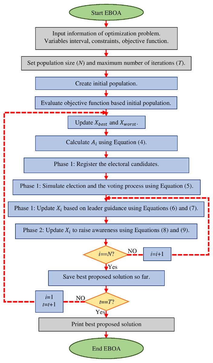
Figure 1: Flowchart of EBOA.
| Start EBOA. |
| Input problem information: variables, objective function, and constraints. |
| Set EBOA population size (N) and iterations (T). |
| Generate the initial population matrix at random. |
| Evaluate the objective function. |
| For t= 1 to T |
| Update best and worst population members. |
| Phase 1: Voting process and holding elections (exploration). |
| Calculate A using Eq. (4). |
| Determine candidates based on awareness criteria. |
| Simulate holding election and voting using Eq. (5). |
| Count the votes and determine the election winner as leader. |
| For i= 1 to N |
| Calculate using Eq. (6). |
| Update Xi using Eq. (7). |
| Phase 2: Public movement to raise awareness (exploitation). |
| Calculate using Eq. (8). |
| Update Xi using Eq. (9). |
| end |
| Save best proposed solution so far. |
| end |
| Output best quasi-optimal solution obtained with the EBOA. |
| End EBOA. |
Computational complexity of EBOA
This subsection is devoted to examining the computational complexity of the EBOA. The computational complexity of EBOA initialization, including random population generation and initial evaluation of the objective function, is equal to O(Nm)where N is the size of the EBOA population and m is the number of problem variables. Holding the election and updating the EBOA population in the first phase has the computational complexity equal to O(NmT) where T is the number of iterations. Population update based on the second phase of EBOA to increase people’s awareness is equal to O(NmT). Accordingly, the total computational complexity of EBOA is equal to O(Nm(1 + 2T)).
Results
This section is dedicated to analyzing EBOA performance in optimization and its ability to provide solutions to problems. Thirty-three objective functions of different types have been selected to evaluate different aspects of the proposed approach. Information and details of these benchmark functions are specified in Tables 1, 2, 3 and 4. The reasons for selecting these objective functions are as follows: functions F1 to F7 are selected as a unimodal type. These types of functions have only one extremum in their search space and are suitable in this regard to evaluate the EBOA’s exploitation ability in local search and converge to this optimal position. Therefore, the reason for choosing unimodal functions is to evaluate the exploitation potential of EBOA. The high-dimensional multimodal functions F8 to F13 include numerous local extremums in their search space in addition to the main extremum. These local optimal situations may cause the algorithm to fail. This feature has adapted the functions F8 to F13 to analyze the EBOA’s exploration ability in global search and determine whether the proposed approach is able to bypass local optimal locations and identify the original optimal location. Therefore, the reason for choosing high-dimensional multimodal functions is to evaluate the EBOA exploration capability. Fixed-dimensional multimodal functions F14 to F23 have fewer local optimal locations in their search space. These types of functions are great criteria for simultaneously measuring exploration and exploitation in optimization methods. Therefore, the reason for choosing fixed-dimensional multimodal functions is to evaluate the EBOA’s ability to strike the balance between the powers of exploration and exploitation. In addition to the twenty-three classic F1 to F23 objective functions, EBOA performance on ten complexes CEC 2019 suite test functions (known as the 100-Digit Challenge Test Functions) is also tested. More information and details about CEC 2019 test functions are available in Price et al. (2018).
| Objective function | Range | Dimensions | Fmin | |
|---|---|---|---|---|
| 1. | 30 | 0 | ||
| 2. | 30 | 0 | ||
| 3. | 30 | 0 | ||
| 4. | 30 | 0 | ||
| 5. | 30 | 0 | ||
| 6. | 30 | 0 | ||
| 7. | 30 | 0 | ||
| Objective function | Range | Dimensions | Fmin | |
|---|---|---|---|---|
| 8. | 30 | −1.2569E +04 | ||
| 9. | 30 | 0 | ||
| 10. | 30 | 0 | ||
| 11. | 30 | 0 | ||
| 12. | 30 | 0 | ||
| 13. | [ − 50, 50] | 30 | 0 | |
| Objective function | Range | Dimensions | Fmin | |
|---|---|---|---|---|
| 14. | 2 | 0.998 | ||
| 15. | 4 | 0.00030 | ||
| 16. | 2 | −1.0316 | ||
| 17. | [ − 5, 10] × [0, 15] | 2 | 0.398 | |
| 18. | 2 | 3 | ||
| 19. | 3 | −3.86 | ||
| 20. | 6 | −3.22 | ||
| 21. | 4 | −10.1532 | ||
| 22. | 4 | −10.4029 | ||
| 23. | 4 | −10.5364 | ||
| Objective function | Range | Dimensions | Fmin | |
|---|---|---|---|---|
| 1. | Storn’s Chebyshev Polynomial Fitting Problem | 9 | 1 | |
| 2. | Inverse Hilbert Matrix Problem | 16 | 1 | |
| 3. | Lennard-Jones Minimum Energy Cluster | 18 | 1 | |
| 4. | Rastrigin’s Function | [ − 100, 100] | 10 | 1 |
| 5. | Griewangk’s Function | [ − 100, 100] | 10 | 1 |
| 6. | Weierstrass Function | [ − 100, 100] | 10 | 1 |
| 7. | Modified Schwefel’s Function | [ − 100, 100] | 10 | 1 |
| 8. | Expanded Schaffer’s F6 Function | [ − 100, 100] | 10 | 1 |
| 9. | Happy Cat Function | [ − 100, 100] | 10 | 1 |
| 10. | Ackley Function | [ − 100, 100] | 10 | 1 |
The quality of the EBOA optimization results is compared with ten state-of-the-art metaheuristic algorithms including (i) the most widely used and oldest methods: GA, PSO, (ii) most cited methods from 2009 to 2014: GSA, TLBO, GWO, (iii) Recently published and widely used methods from 2016 to 2021: WOA, MPA, LPB, FDO, and TSA. As noted in the literature, numerous optimization methods have been developed to date. Comparing the proposed EBOA approach with all of these methods, while possible, generates a hug deal of data. Among the metaheuristic algorithms developed, some methods have attracted more attention due to their high efficiency. For this reason, in this study, the ten mentioned metaheuristic algorithms that have been most considered and used have been selected to compare with the performance of EBOA. The values set for the control parameters of these metaheuristics are listed in Table 5.
| Algorithm | Parameter | Value |
|---|---|---|
| GA | ||
| Type | Real coded. | |
| Selection | Roulette wheel (Proportionate). | |
| Crossover | Whole arithmetic (Probability = 0.8, ) | |
| Mutation | Gaussian (Probability = 0.05). | |
| PSO | ||
| Topology | Fully connected. | |
| Cognitive and social constant | . | |
| Inertia weight | Linear reduction from 0.9 to 0.1 | |
| Velocity limit | 10% of dimension range. | |
| GSA | ||
| Alpha, G0, Rnorm, Rpower | 20, 100, 2, 1 | |
| TLBO | ||
| TF: teaching factor | , | |
| Random number | rand is a random number in interval | |
| GWO | ||
| Convergence parameter (a) | a: Linear reduction from 2 to 0. | |
| WOA | ||
| Convergence parameter (a) | a: Linear reduction from 2 to 0. | |
| r | r is a vector of random numbers in | |
| l | l is a random number in | |
| TSA | ||
| Pmin and P max | 1 and 4 | |
| c1, c2, c3 | Random numbers lie in the range from 0 to 1. | |
| MPA | ||
| Constant number | P = 0.5, | |
| Random vector | R is a vector of uniform random numbers in the interval | |
| Fish Aggregating Devices (FADs) | FADs = 0.2 | |
| Binary vector | U = 0 or 1 | |
| FDO | ||
| Weight factor wf | wf is either 0 or 1 | |
| r | r is a vector of random numbers in 0,1. | |
| LPB | ||
| Crossover Percentage | pc = 0.6, | |
| Number of Offsprings (Parnets) | nc = 2 ⋅round(pc⋅nPop/2), | |
| Mutation Percentage | pm = 0.3, | |
| Number of Mutants | nm = round(pm⋅nPop), | |
| Mutation Rate | mu = 0.03, | |
| Divide probability | dp = 0.5, | |
| beta = 8 | ||
| gamma = 0.05 |
The EBOA and ten competitor metaheuristics are each employed in twenty independent implementations to solve the objective functions F1 to F23, while each implementation contains 1,000 repetitions. The termination condition can be based on various criteria such as number of iterations, number of function evaluations, the error between several consecutive iterations, and other cases. In this study, the termination condition is considered based on the number of iterations. The experiments are performed in the Matlab R2020a version in the environment of Microsoft Windows 10 with 64 bits on the Core i-7 processor with 2.40 GHz and 6 GB memory. Simulation results and performance of metaheuristic algorithms are reported using five indicators: mean, best proposed solution, standard deviation (std), median, and rank.
Evaluation unimodal objective function
The results of applying EBOA and ten competitor metaheuristic algorithms to optimize F1 to F7 unimodal functions are reported in Table 6. The optimization outputs show the EBOA has provided the global optimal in solving the F1, F3, and F6 functions. EBOA is the first best optimizer in solving F2, F4, F5, and F7. The simulation results show that in handling the F1 to F7 functions, the EBOA performed better than the ten competitor metaheuristic algorithms and ranked first.
| EBOA | FDO | LPB | MPA | TSA | WOA | GWO | TLBO | GSA | PSO | GA | ||
|---|---|---|---|---|---|---|---|---|---|---|---|---|
| F1 | Mean | 0 | 1.27E−31 | 0.6059539 | 1.71E−18 | 8.21E−33 | 1.59E−09 | 1.09E−58 | 1.34E−59 | 2.03E−17 | 1.77E−05 | 13.24063 |
| Best | 0 | 3.29E−34 | 0.1656726 | 5.92E−26 | 1.14E−62 | 1.09E−16 | 7.73E−61 | 9.36E−61 | 8.20E−18 | 2.00E−10 | 5.59388 | |
| std | 0 | 1.96E−31 | 0.2883118 | 6.76E−18 | 2.53E−32 | 3.22E−09 | 4.09E−58 | 2.05E−59 | 7.10E−18 | 5.86E−05 | 5.72729 | |
| Median | 0 | 2.61E−32 | 0.552771 | 1.63E−19 | 6.83E−40 | 1.09E−09 | 1.08E−59 | 4.69E−60 | 1.78E−17 | 9.93E−07 | 11.04546 | |
| Rank | 1 | 5 | 10 | 6 | 4 | 8 | 3 | 2 | 7 | 9 | 11 | |
| F2 | Mean | 1.30E−261 | 3.26E−16 | 0.2088937 | 2.78E−09 | 5.02E−39 | 0.538136 | 1.30E−34 | 5.55E−35 | 2.37E−08 | 0.341139 | 2.479432 |
| Best | 8.30E−271 | 3.19E−17 | 0.1002184 | 4.25E−18 | 8.26E−43 | 0.461308 | 1.55E−35 | 1.32E−35 | 1.59E−08 | 0.001741 | 1.591248 | |
| std | 0 | 3.87E−16 | 0.0757105 | 1.08E−08 | 1.72E−38 | 0.048065 | 2.20E−34 | 4.71E−35 | 3.96E−09 | 0.669594 | 0.642843 | |
| Median | 3.50E−265 | 1.79E−16 | 0.1831153 | 3.18E−11 | 8.26E−41 | 0.545056 | 6.38E−35 | 4.37E−35 | 2.33E−08 | 0.130114 | 2.463873 | |
| Rank | 1 | 5 | 8 | 6 | 2 | 10 | 4 | 3 | 7 | 9 | 11 | |
| F3 | Mean | 0 | 0.8016065 | 5116.4258 | 0.377013 | 3.20E−19 | 9.94E−08 | 7.41E−15 | 7.01E−15 | 279.3468 | 589.4942 | 1536.915 |
| Best | 0 | 0.0148424 | 2992.3972 | 0.032038 | 7.29E−30 | 1.74E−12 | 4.75E−20 | 1.21E−16 | 81.91242 | 1.614937 | 1014.689 | |
| std | 0 | 1.8545893 | 1727.1652 | 0.201758 | 9.90E−19 | 3.87E−07 | 1.90E−14 | 1.27E−14 | 112.3057 | 1524.007 | 367.2108 | |
| Median | 0 | 0.2027959 | 5275.2084 | 0.378658 | 9.81E−21 | 1.74E−08 | 1.59E−16 | 1.86E−15 | 291.441 | 54.15445 | 1510.715 | |
| Rank | 1 | 7 | 11 | 6 | 2 | 5 | 4 | 3 | 8 | 9 | 10 | |
| F4 | Mean | 5.30E−260 | 0.8309008 | 2.9453299 | 3.66E−08 | 2.01E−22 | 5.10E−05 | 1.26E−14 | 1.58E−15 | 3.25E−09 | 3.963461 | 2.094271 |
| Best | 3.10E−266 | 0.211467 | 2.0418994 | 3.42E−17 | 1.87E−52 | 7.34E−06 | 3.43E−16 | 6.42E−16 | 2.09E−09 | 1.604522 | 1.389849 | |
| std | 0 | 0.5440558 | 0.5030838 | 6.45E−08 | 5.96E−22 | 5.74E−05 | 2.32E−14 | 7.14E−16 | 7.50E−10 | 2.204083 | 0.337011 | |
| Med | 2.10E−262 | 0.7476137 | 2.8820789 | 3.03E−08 | 3.13E−27 | 3.45E−05 | 7.30E−15 | 1.54E−15 | 3.34E−09 | 3.260791 | 2.09854 | |
| Rank | 1 | 8 | 10 | 6 | 2 | 7 | 4 | 3 | 5 | 11 | 9 | |
| F5 | Mean | 25.91771 | 45.546797 | 163.70642 | 42.49778 | 28.76746 | 41.15923 | 26.86099 | 145.6667 | 36.10723 | 50.26311 | 310.4313 |
| Best | 24.94581 | 19.180105 | 95.107228 | 41.58682 | 28.53831 | 39.3088 | 25.21377 | 120.7932 | 25.83811 | 3.647051 | 160.5013 | |
| std | 0.433265 | 37.836937 | 41.043291 | 0.615521 | 0.364773 | 0.489502 | 0.884088 | 19.73905 | 32.46252 | 36.52379 | 120.4473 | |
| Median | 26.13112 | 22.222915 | 166.09256 | 42.49068 | 28.54102 | 41.3088 | 26.70967 | 142.8987 | 26.07475 | 28.69395 | 279.5174 | |
| Rank | 1 | 7 | 10 | 6 | 3 | 5 | 2 | 9 | 4 | 8 | 11 | |
| F6 | Mean | 0 | 4.93E−21 | 0.05 | 0.390872 | 3.84E−20 | 2.53E−09 | 0.642334 | 0.45 | 0 | 20.2502 | 14.5501 |
| Best | 0 | 1.92E−23 | 0 | 0.274582 | 6.74E−26 | 1.95E−15 | 1.57E−05 | 0 | 0 | 5 | 6.00042 | |
| std | 0 | 9.71E−21 | 0.2236068 | 0.080282 | 1.50E−19 | 4.05E−09 | 0.301088 | 0.510418 | 0 | 12.77311 | 5.835177 | |
| Median | 0 | 1.41E−21 | 0 | 0.406648 | 6.74E−21 | 1.95E−09 | 0.621487 | 0 | 0 | 19 | 13.5 | |
| Rank | 1 | 2 | 5 | 6 | 3 | 4 | 8 | 7 | 1 | 10 | 9 | |
| F7 | Mean | 4.77E−05 | 0.8072237 | 0.0718038 | 0.002182 | 0.000276 | 0.01946 | 0.000819 | 0.00313 | 0.020692 | 0.113415 | 0.00568 |
| Best | 9.87E−07 | 0.2679768 | 0.0318638 | 0.001429 | 0.000104 | 0.002027 | 0.000248 | 0.001362 | 0.01006 | 0.029593 | 0.002111 | |
| std | 4.40E−05 | 0.3625883 | 0.0221458 | 0.000466 | 0.000123 | 0.004115 | 0.000503 | 0.001351 | 0.01136 | 0.045868 | 0.002433 | |
| Median | 3.56E−05 | 0.8273515 | 0.0719665 | 0.00218 | 0.000367 | 0.020272 | 0.000629 | 0.002912 | 0.016996 | 0.107872 | 0.005365 | |
| Rank | 1 | 11 | 9 | 4 | 2 | 7 | 3 | 5 | 8 | 10 | 6 | |
| Sum rank | 7 | 45 | 63 | 40 | 18 | 46 | 28 | 32 | 40 | 66 | 67 | |
| Mean rank | 1 | 6.4285 | 9 | 5.7142 | 2.5714 | 6.5714 | 4 | 4.5714 | 5.7142 | 9.4285 | 9.5714 | |
| Total rank | 1 | 6 | 8 | 5 | 2 | 7 | 3 | 4 | 5 | 9 | 10 | |
Evaluation of high-dimensional multimodal objective functions
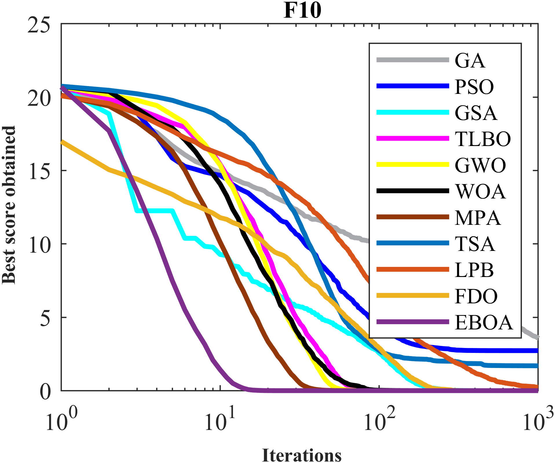
The optimization results of F8 to F13 functions obtained from the implementation of EBOA and ten competing metaheuristic algorithms are released in Table 6. EBOA is able to converge to the global optimum in handling F9 and F11 functions. In optimizing the F10, F12, F13, and F14 functions, what is evident from the simulation results is that EBOA is the first best optimizer in these functions. In optimizing the F8 function, after GA and TLBO, the proposed EBOA is the third best optimizer of this function. What can be deduced from the results of Table 7 is that EBOA has a higher capability in optimizing high-dimensional multimodal functions compared to ten competitor algorithms and is ranked first as the best optimizer in functions 8 to F13.
| EPOA | FDO | LPB | MPA | TSA | WOA | GWO | TLBO | GSA | PSO | GA | ||
|---|---|---|---|---|---|---|---|---|---|---|---|---|
| F8 | Mean | −7149.45 | −6742.4711 | −11057.297 | −3652.09 | −5669.56 | −1633.55 | −5885.02 | −7803.47 | −2849.03 | −6908.54 | −8184.3 |
| Best | −8600.95 | −7688.9971 | −11972.938 | −4419.9 | −5706.3 | −2358.57 | −7227.05 | −9103.77 | −3969.23 | −8500.59 | −9717.68 | |
| std | 720.2391 | 385.42421 | 340.85937 | 474.608 | 21.84579 | 374.5924 | 984.4547 | 986.5806 | 540.379 | 836.6452 | 795.1826 | |
| Median | −7123.95 | −6794.0493 | −11028.692 | −3632.65 | −5669.63 | −1649.72 | −5774.63 | −7735.22 | −2671.33 | −7098.95 | −8117.25 | |
| Rank | 4 | 6 | 1 | 9 | 8 | 11 | 7 | 3 | 10 | 5 | 2 | |
| F9 | Mean | 0 | 12.106148 | 0.4418522 | 152.6934 | 0.005888 | 3.666025 | 8.53E−15 | 10.67763 | 16.26778 | 57.06189 | 62.41204 |
| Best | 0 | 5.7972799 | 0.0558848 | 128.2306 | 0.004776 | 1.78099 | 0 | 9.873963 | 4.974795 | 27.85883 | 36.86623 | |
| std | 0 | 4.3697476 | 0.2628465 | 15.18316 | 0.000696 | 1.07177 | 2.08E−14 | 0.397117 | 4.658816 | 16.51737 | 15.21563 | |
| Median | 0 | 10.939576 | 0.3549152 | 154.6214 | 0.005871 | 3.78099 | 0 | 10.88657 | 15.42242 | 55.22468 | 61.67858 | |
| Rank | 1 | 7 | 4 | 11 | 3 | 5 | 2 | 6 | 8 | 9 | 10 | |
| F10 | Mean | 1.24E−15 | 8.76E−12 | 0.2378952 | 8.31E−10 | 6.38E−11 | 0.279162 | 1.71E−14 | 0.263208 | 3.57E−09 | 2.154699 | 3.221863 |
| Best | 8.88E−16 | 1.22E−13 | 0.1155122 | 1.68E−18 | 8.14E−15 | 0.013128 | 1.51E−14 | 0.156316 | 2.64E−09 | 1.155151 | 2.757203 | |
| std | 1.09E−15 | 2.47E−11 | 0.0933506 | 2.80E−09 | 2.60E−10 | 0.146961 | 3.15E−15 | 0.072865 | 5.27E−10 | 0.549446 | 0.361797 | |
| Median | 8.88E−16 | 2.53E−12 | 0.2136625 | 1.05E−11 | 1.10E−13 | 0.312835 | 1.51E−14 | 0.261541 | 3.64E−09 | 2.170083 | 3.120322 | |
| Rank | 1 | 3 | 7 | 5 | 4 | 9 | 2 | 8 | 6 | 10 | 11 | |
| F11 | Mean | 0 | 0.0167647 | 0.5041482 | 0 | 1.55E−06 | 0.105702 | 0.003753 | 0.587689 | 3.737598 | 0.046293 | 1.230221 |
| Best | 0 | 0 | 0.2403442 | 0 | 4.23E−15 | 0.08107 | 0 | 0.310117 | 1.519288 | 7.29E−09 | 1.140551 | |
| std | 0 | 0.0174995 | 0.19818 | 0 | 3.38E−06 | 0.007345 | 0.007344 | 0.169117 | 1.670282 | 0.051834 | 0.062756 | |
| Median | 0 | 0.0091183 | 0.4827497 | 0 | 8.77E−07 | 0.10701 | 0 | 0.582026 | 3.424268 | 0.029473 | 1.227231 | |
| Rank | 1 | 4 | 7 | 1 | 2 | 6 | 3 | 8 | 10 | 5 | 9 | |
| F12 | Mean | 2.71E−07 | 0.027568 | 0.0050244 | 0.082559 | 0.050164 | 1.557746 | 0.037211 | 0.020551 | 0.036283 | 0.480672 | 0.047027 |
| Best | 1.63E−07 | 9.02E−23 | 0.0003721 | 0.077912 | 0.035428 | 0.56726 | 0.019295 | 0.002031 | 5.57E−20 | 0.000145 | 0.018364 | |
| std | 5.25E−08 | 0.0463417 | 0.009498 | 0.002386 | 0.009855 | 0.4596 | 0.013875 | 0.028645 | 0.060866 | 0.602582 | 0.028483 | |
| Median | 2.70E−07 | 3.21E−07 | 0.0010168 | 0.082111 | 0.050935 | 1.56726 | 0.032991 | 0.015181 | 1.48E−19 | 0.1556 | 0.04179 | |
| Rank | 1 | 4 | 2 | 9 | 8 | 11 | 6 | 3 | 5 | 10 | 7 | |
| F13 | Mean | 3.88E−06 | 5.49E−05 | 0.0307545 | 0.565254 | 2.658778 | 0.338392 | 0.576327 | 0.329124 | 0.002085 | 0.508412 | 1.208556 |
| Best | 2.00E−06 | 4.55E−21 | 0.0064812 | 0.280295 | 2.63175 | 0.332688 | 0.297822 | 0.038266 | 1.18E−18 | 9.99E−07 | 0.49809 | |
| std | 9.01E−07 | 0.000202 | 0.0215577 | 0.187817 | 0.009796 | 0.001343 | 0.170359 | 0.198939 | 0.005476 | 1.251681 | 0.333754 | |
| Median | 3.79E−06 | 2.09E−17 | 0.0276489 | 0.579874 | 2.66175 | 0.338688 | 0.578323 | 0.282784 | 2.14E−18 | 0.043997 | 1.218096 | |
| Rank | 1 | 2 | 4 | 8 | 11 | 6 | 9 | 5 | 3 | 7 | 10 | |
| Sum rank | 9 | 26 | 25 | 43 | 36 | 48 | 29 | 33 | 42 | 46 | 49 | |
| Mean rank | 1.5 | 4.3333333 | 4.1666667 | 7.1666667 | 6 | 8 | 4.8333333 | 5.5 | 7 | 7.6666667 | 8.1666667 | |
| Total rank | 1 | 3 | 2 | 8 | 6 | 10 | 4 | 5 | 7 | 9 | 11 | |
| EBOA | FDO | LPB | MPA | TSA | WOA | GWO | TLBO | GSA | PSO | GA | ||
|---|---|---|---|---|---|---|---|---|---|---|---|---|
| F14 | Mean | 0.998004 | 1.3459133 | 0.998004 | 0.998998 | 1.798757 | 1.043798 | 3.740858 | 2.264292 | 3.591435 | 2.173601 | 0.99867 |
| Best | 0.998004 | 0.9980038 | 0.998004 | 0.998137 | 0.998004 | 0.998004 | 0.998004 | 0.998391 | 0.999508 | 0.998004 | 0.998004 | |
| std | 9.23E−14 | 0.4864376 | 1.10E−10 | 0.000324 | 0.527414 | 0.204528 | 3.969726 | 1.149621 | 2.778791 | 2.936536 | 0.002471 | |
| Median | 0.998004 | 0.9980038 | 0.998004 | 0.999138 | 1.912608 | 0.998004 | 2.982105 | 2.275231 | 2.986658 | 0.998004 | 0.998027 | |
| Rank | 1 | 5 | 1 | 3 | 6 | 4 | 10 | 8 | 9 | 7 | 2 | |
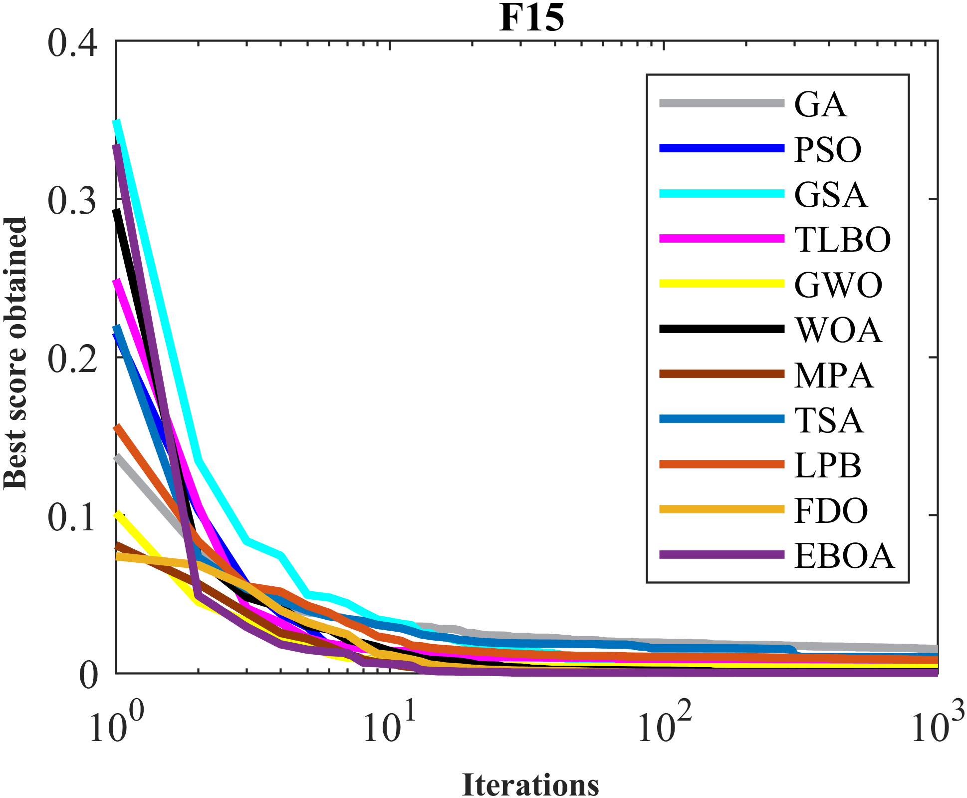
| F15 | Mean | 0.000308 | 0.0003138 | 0.0085214 | 0.003936 | 0.000408 | 0.003719 | 0.00637 | 0.003169 | 0.002402 | 0.001684 | 0.005395 |
| Best | 0.000307 | 0.0003075 | 0.0004878 | 0.00027 | 0.000264 | 0.000441 | 0.000307 | 0.002206 | 0.000805 | 0.000307 | 0.000775 | |
| std | 3.30E−07 | 2.61E−05 | 0.0092568 | 0.005051 | 7.59E−05 | 0.001248 | 0.009401 | 0.000394 | 0.001195 | 0.004932 | 0.0081 | |
| Median | 0.000308 | 0.0003075 | 0.0022942 | 0.0027 | 0.00039 | 0.00441 | 0.000308 | 0.003185 | 0.002311 | 0.000307 | 0.002074 | |
| Rank | 1 | 2 | 11 | 8 | 3 | 7 | 10 | 6 | 5 | 4 | 9 | |
| F16 | Mean | −1.03163 | −1.0316285 | −1.0316273 | −1.03157 | −1.03158 | −1.03158 | −1.03161 | −1.03161 | −1.03161 | −1.03161 | −1.0316 |
| Best | −1.03163 | −1.0316285 | −1.0316285 | −1.0316 | −1.03161 | −1.0316 | −1.03163 | −1.03163 | −1.03163 | −1.03163 | −1.03163 | |
| std | 1.14E−10 | 7.75E−10 | 2.19E−06 | 4.42E−05 | 4.09E−05 | 3.78E−05 | 3.78E−05 | 3.78E−05 | 3.78E−05 | 3.78E−05 | 4.92E−05 | |
| Median | −1.03163 | −1.0316285 | −1.0316281 | −1.0316 | −1.0316 | −1.0316 | −1.03163 | −1.03163 | −1.03163 | −1.03163 | −1.03162 | |
| Rank | 1 | 2 | 3 | 7 | 6 | 6 | 4 | 4 | 4 | 4 | 5 | |
| F17 | Mean | 0.397887 | 0.3978875 | 0.3979073 | 0.399302 | 0.400093 | 0.405055 | 0.397894 | 0.397892 | 0.397892 | 0.785448 | 0.436972 |
| Best | 0.397887 | 0.3978874 | 0.3978875 | 0.39757 | 0.398052 | 0.399405 | 0.397887 | 0.397887 | 0.397887 | 0.397887 | 0.397888 | |
| std | 3.28E−09 | 3.04E−07 | 2.95E−05 | 0.003672 | 0.00448 | 0.003664 | 1.02E−05 | 1.02E−05 | 1.02E−05 | 0.721752 | 0.140745 | |
| Median | 0.397887 | 0.3978874 | 0.3978944 | 0.39782 | 0.399052 | 0.40466 | 0.397888 | 0.397887 | 0.397887 | 0.397915 | 0.397925 | |
| Rank | 1 | 2 | 5 | 6 | 7 | 8 | 4 | 3 | 3 | 10 | 9 | |
| F18 | Mean | 3 | 3 | 3.0000232 | 3.000032 | 3.093107 | 3.000228 | 3.000042 | 3.000031 | 3.000031 | 3.000031 | 4.359425 |
| Best | 3 | 3 | 3.0000003 | 3 | 2.999974 | 3.000149 | 3 | 3 | 3 | 3 | 3.000001 | |
| std | 0 | 1.49E−11 | 2.64E−05 | 7.69E−05 | 0.031851 | 0.000126 | 7.76E−05 | 7.69E−05 | 7.69E−05 | 7.69E−05 | 6.035694 | |
| Median | 3 | 3 | 3.0000109 | 3 | 3.103419 | 3.000149 | 3.000007 | 3 | 3 | 3 | 3.001083 | |
| Rank | 1 | 1 | 2 | 4 | 7 | 6 | 5 | 3 | 3 | 3 | 8 | |
| F19 | Mean | −3.86278 | −3.86278 | −3.86278 | −3.86264 | −3.80654 | −3.8616 | −3.86211 | −3.86132 | −3.86272 | −3.86272 | −3.85428 |
| Best | −3.86278 | −3.86278 | −3.86278 | −3.8627 | −3.8366 | −3.86276 | −3.86278 | −3.8625 | −3.86278 | −3.86278 | −3.86278 | |
| std | 3.38E−07 | 5.74E−06 | 2.05E−07 | 0.000142 | 0.015257 | 0.003062 | 0.001704 | 0.001374 | 0.000142 | 0.000142 | 0.014852 | |
| Median | −3.86278 | −3.86278 | −3.86278 | −3.8627 | −3.8066 | −3.86266 | −3.86275 | −3.86187 | −3.86278 | −3.86278 | −3.86226 | |
| Rank | 1 | 1 | 1 | 3 | 8 | 5 | 4 | 6 | 2 | 2 | 7 | |
| F20 | Mean | −3.322 | −3.3219846 | −3.274437 | −3.32105 | −3.31947 | −3.23224 | −3.25234 | −3.20112 | −3.32195 | −3.2619 | −2.82386 |
| Best | −3.322 | −3.321995 | −3.3219951 | −3.3213 | −3.3212 | −3.31342 | −3.32199 | −3.26174 | −3.322 | −3.322 | −3.31342 | |
| std | 9.99E−08 | 1.16E−05 | 0.0597588 | 0.000147 | 0.003069 | 0.035652 | 0.076565 | 0.031823 | 0.000122 | 0.070623 | 0.385958 | |
| Median | −3.322 | −3.3219895 | −3.3219932 | −3.3211 | −3.32058 | −3.2424 | −3.26231 | −3.20744 | −3.322 | −3.32166 | −2.96828 | |
| Rank | 1 | 2 | 6 | 4 | 5 | 9 | 8 | 10 | 3 | 7 | 11 | |
| F21 | Mean | −10.1532 | −10.150391 | −5.642384 | −9.95429 | −5.40202 | −7.40498 | −9.64509 | −9.19003 | −5.14855 | −5.38916 | −4.30394 |
| Best | −10.1532 | −10.153199 | −10.153196 | −10.1532 | −7.50209 | −7.48159 | −10.1532 | −9.66387 | −10.1532 | −10.1532 | −7.82781 | |
| std | 2.33E−06 | 0.003942 | 3.4984609 | 0.532557 | 0.967922 | 0.03346 | 1.561937 | 0.120744 | 3.054458 | 3.019762 | 1.740798 | |
| Median | −10.1532 | −10.152212 | −3.8690264 | −10.1532 | −5.50209 | −7.40159 | −10.1526 | −9.1532 | −3.64784 | −5.10077 | −4.16197 | |
| Rank | 1 | 2 | 7 | 3 | 8 | 6 | 4 | 5 | 10 | 9 | 11 | |
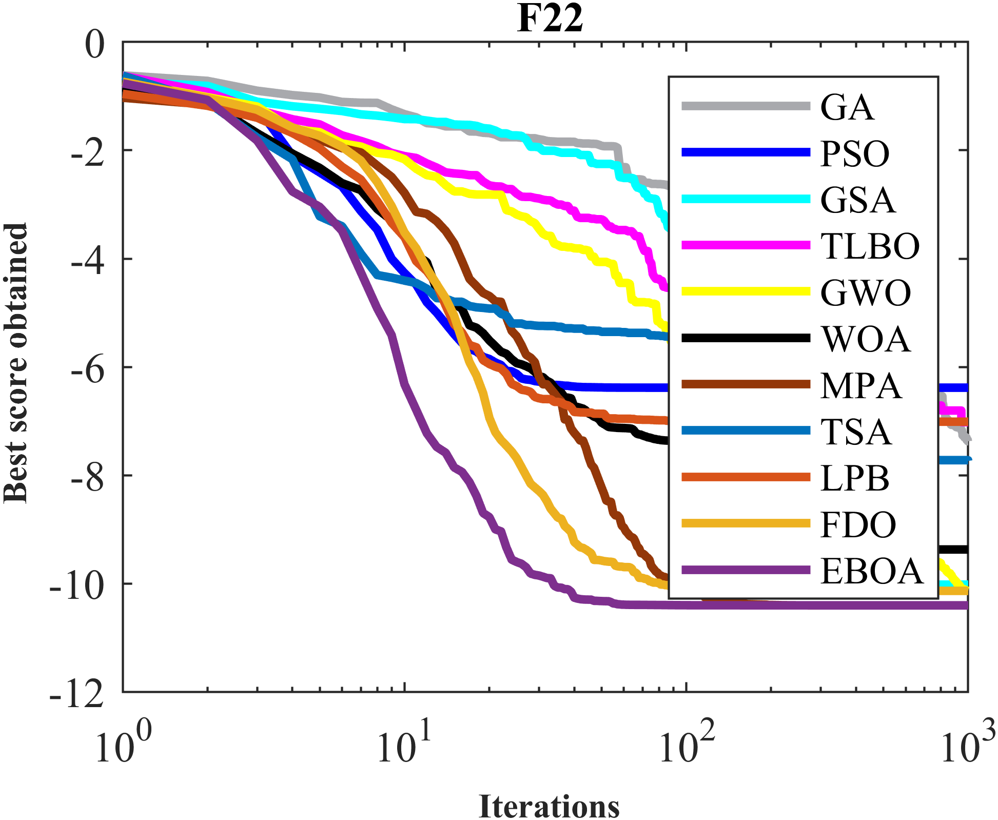
| F22 | Mean | −10.4029 | −10.134399 | −7.01164 | −10.2858 | −5.9134 | −8.6996 | −10.4024 | −10.0485 | −10.0846 | −7.63218 | −5.11734 |
| Best | −10.4029 | −10.402939 | −10.402941 | −10.4029 | −9.06249 | −10.4029 | −10.4028 | −10.4029 | −10.4029 | −10.4029 | −9.11064 | |
| std | 2.18E−06 | 1.1783516 | 3.5358695 | 0.245334 | 1.754912 | 1.356173 | 0.000474 | 0.398327 | 1.423122 | 3.541608 | 1.969599 | |
| Median | −10.4029 | −10.401725 | −7.7657081 | −10.4027 | −5.06249 | −8.81649 | −10.4025 | −10.1836 | −10.4029 | −10.4019 | −5.0294 | |
| Rank | 1 | 4 | 9 | 3 | 10 | 7 | 2 | 6 | 5 | 8 | 11 | |
| F23 | Mean | −10.5364 | −10.532661 | −6.4463091 | −10.1407 | −9.80971 | −10.0215 | −10.1301 | −9.26415 | −10.5363 | −6.16472 | −6.56203 |
| Best | −10.5364 | −10.536408 | −10.536409 | −10.5364 | −10.3683 | −10.5364 | −10.5363 | −10.534 | −10.5364 | −10.5364 | −10.2216 | |
| std | 3.63E−06 | 0.0062871 | 3.8555684 | 1.140111 | 1.606403 | 0.355828 | 1.814366 | 1.676549 | 0.000386 | 3.734897 | 2.617187 | |
| Median | −10.5364 | −10.535362 | −4.5055122 | −10.5364 | −10.3613 | −10.0003 | −10.5359 | −9.67172 | −10.5364 | −4.50535 | −6.5629 | |
| Rank | 1 | 3 | 10 | 4 | 7 | 6 | 5 | 8 | 2 | 11 | 9 | |
| Sum rank | 10 | 24 | 55 | 45 | 67 | 64 | 56 | 59 | 46 | 65 | 82 | |
| Mean rank | 1 | 2.4 | 5.5 | 4.5 | 6.7 | 6.4 | 5.6 | 5.9 | 4.6 | 6.5 | 8.2 | |
| Total rank | 1 | 2 | 5 | 3 | 10 | 8 | 6 | 7 | 4 | 9 | 11 | |
Evaluation of fixed-dimensional multimodal objective functions
The results obtained from the implementation of EBOA and ten competitor metaheuristic algorithms on F14 to F23 functions are presented in Table 8. What emerges from the simulation output is that EBOA is the first best optimizer to handle F14 to F23 functions. Analysis and comparison of the obtained results indicate that the proposed EBOA approach has a superior performance over ten metaheuristic algorithms and among them, it has the first rank of the best optimizer.
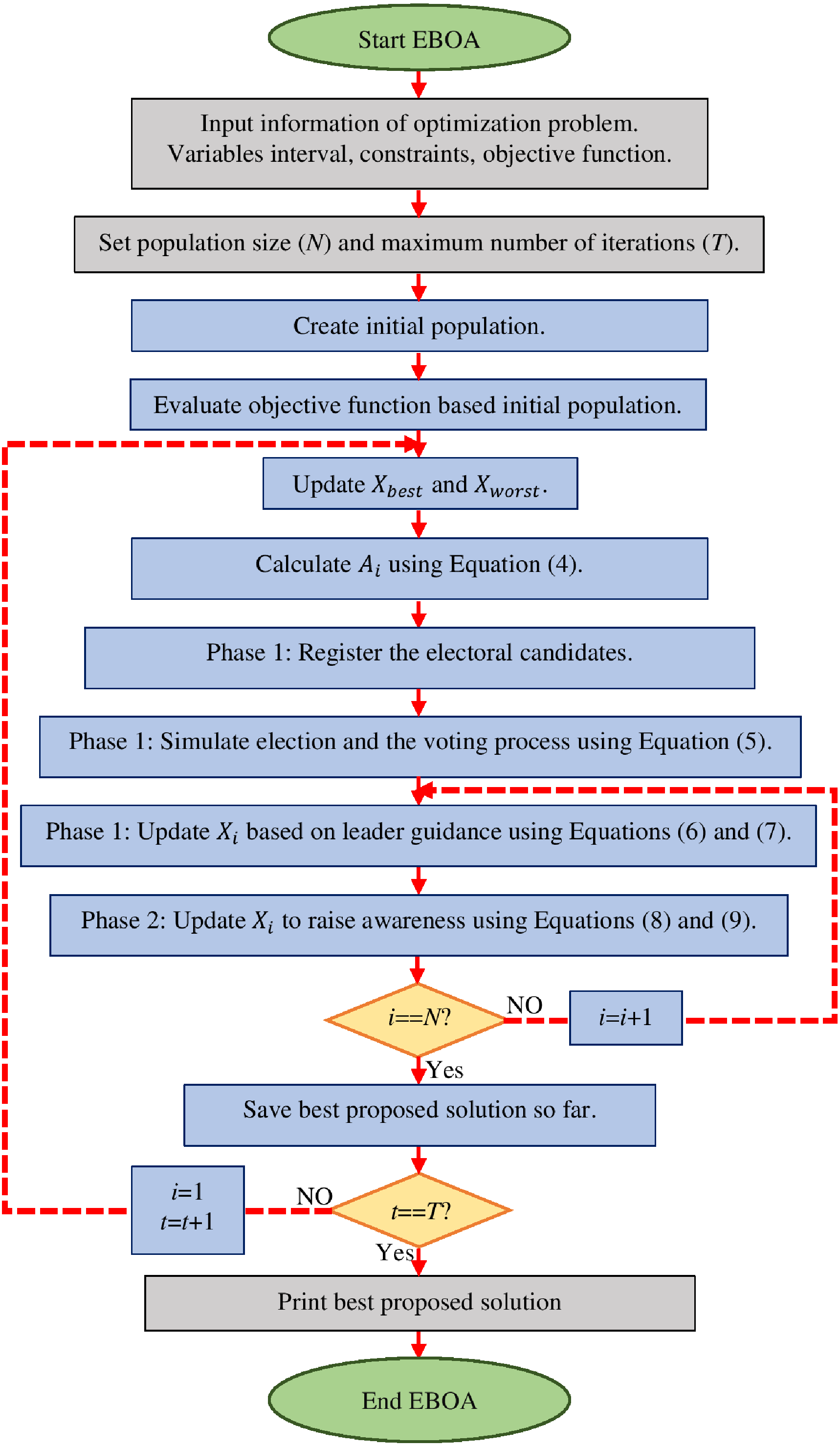
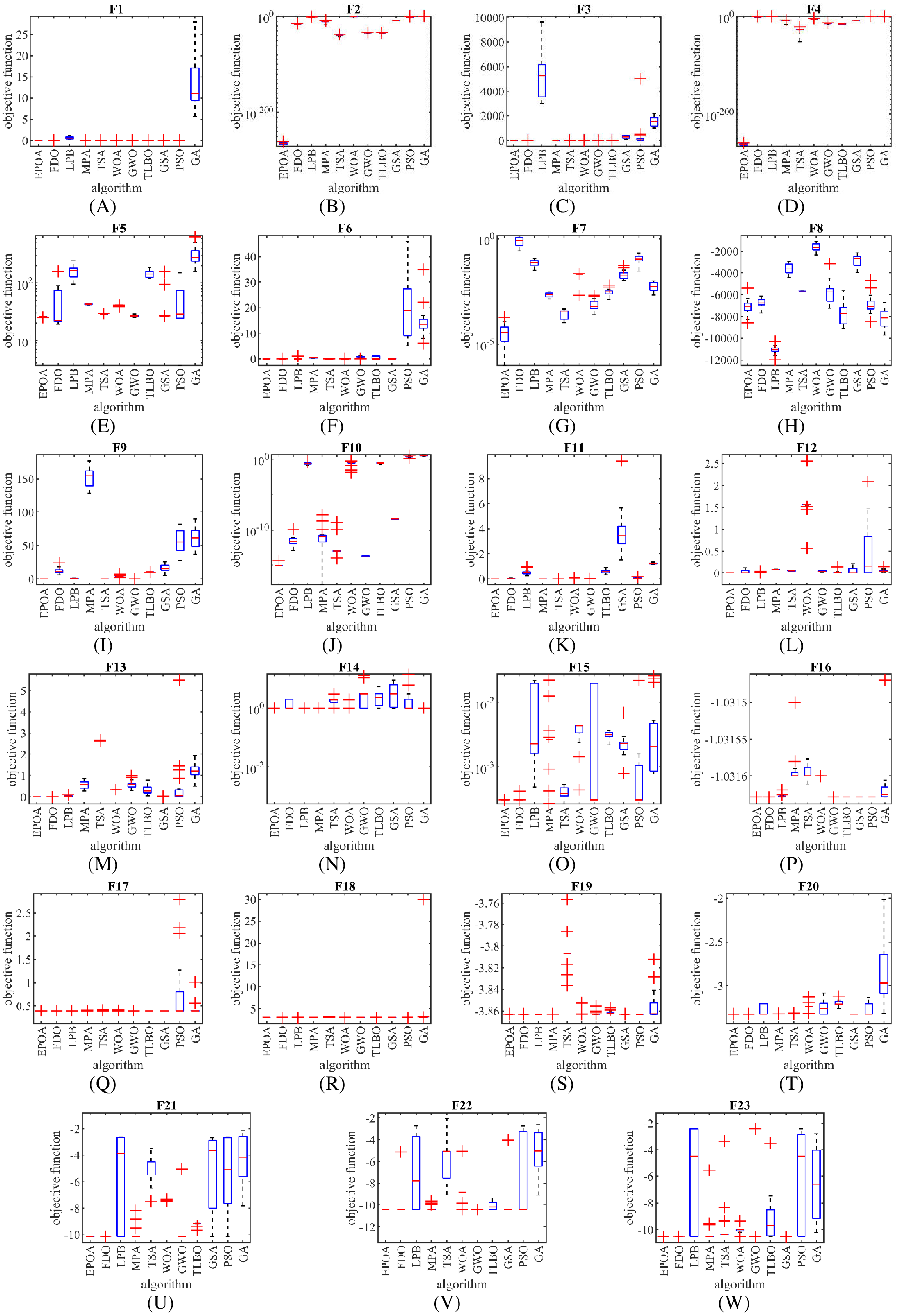
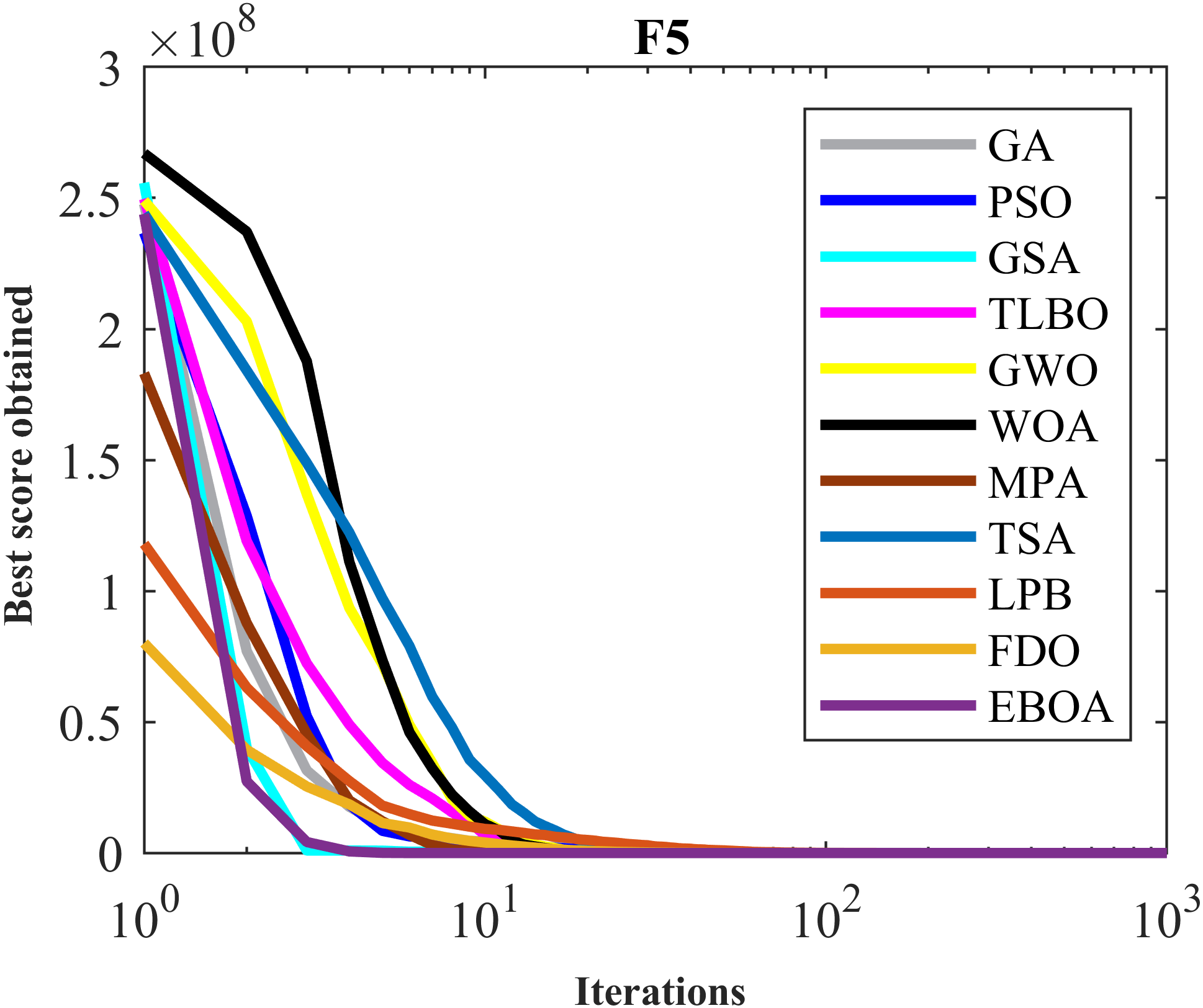
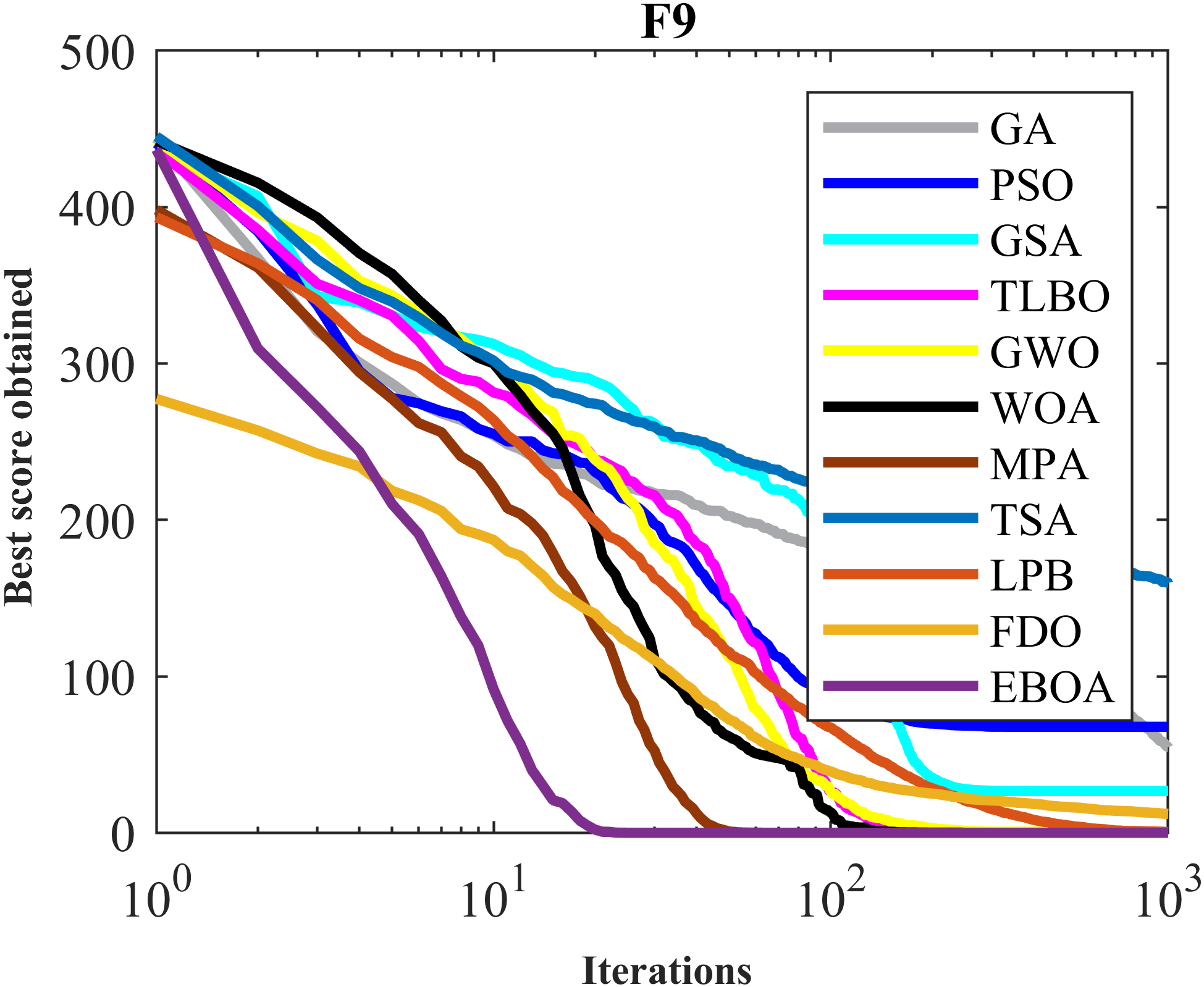
The performance of the EBOA and the ten competitor metaheuristic algorithms implemented on the F1 to F23 objective functions are shown in Fig. 2 as the boxplot. For visual analysis of the ability to achieve the searched solution, Figs. 3 to 11 show the convergence curves of the EBOA and ten other competing algorithms in optimizing a number of objective functions.
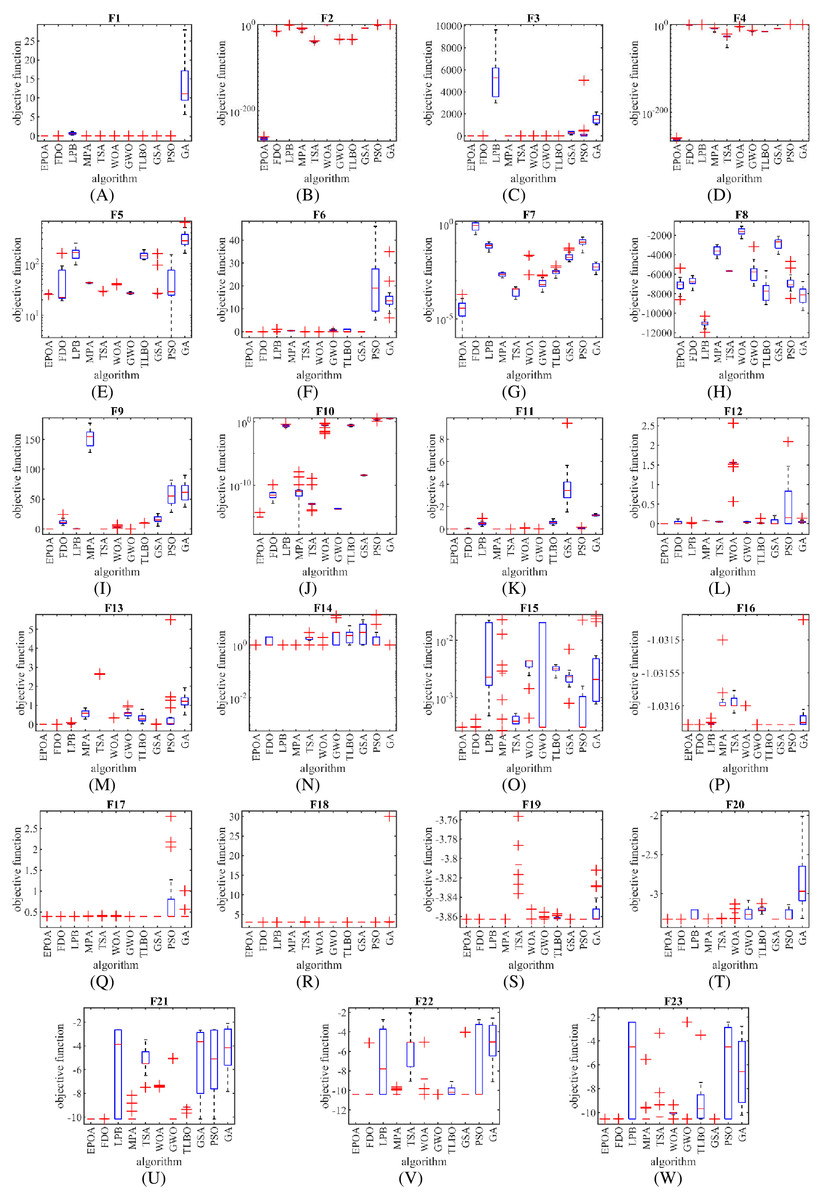
Figure 2: (A–W) Boxplot diagram of EPOA and ten metaheuristic algorithms performances on F1 to F23.
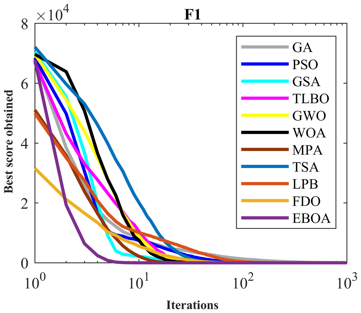
Figure 3: Convergence curves of EPOA and competitor algorithms on F1.
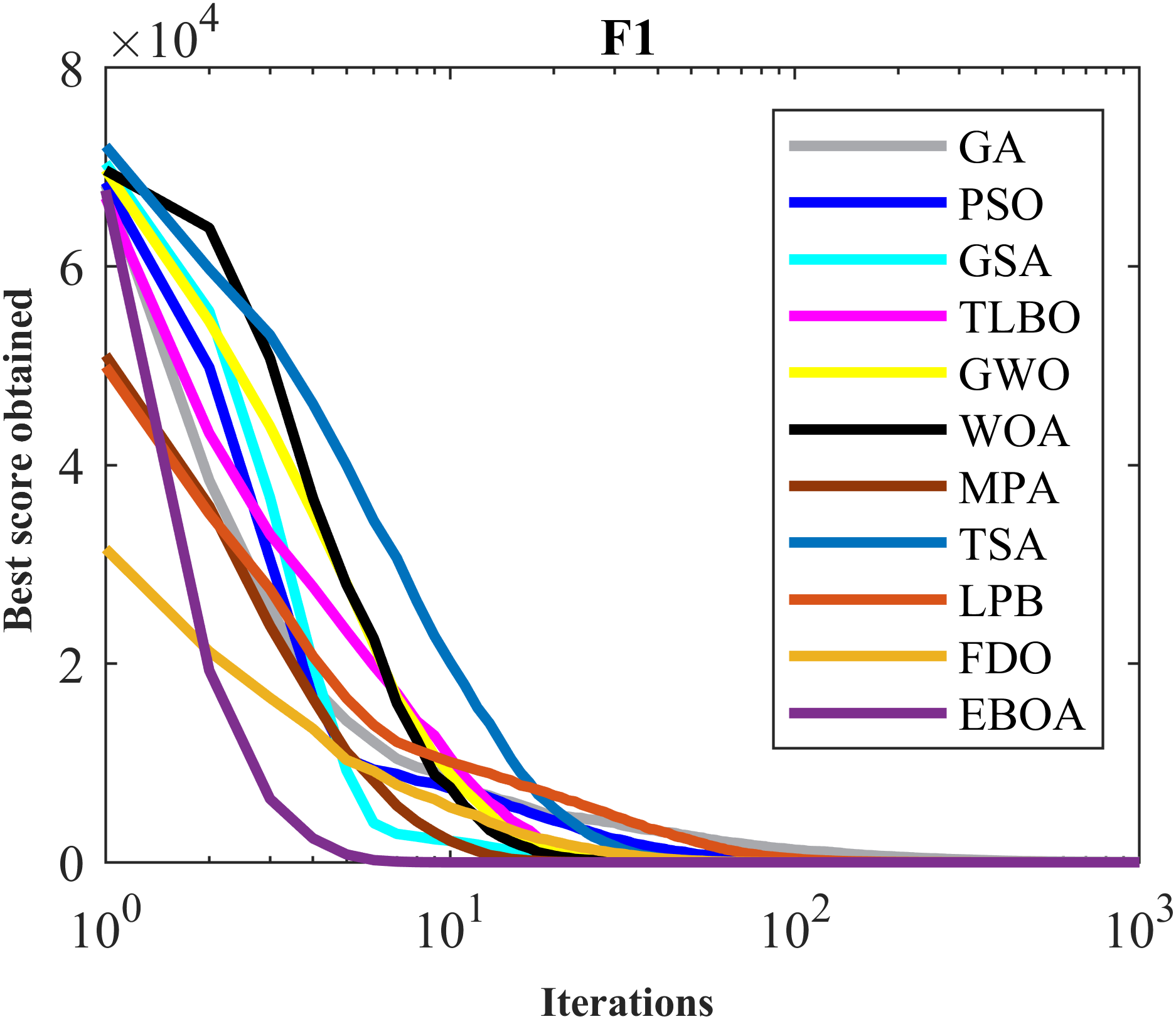
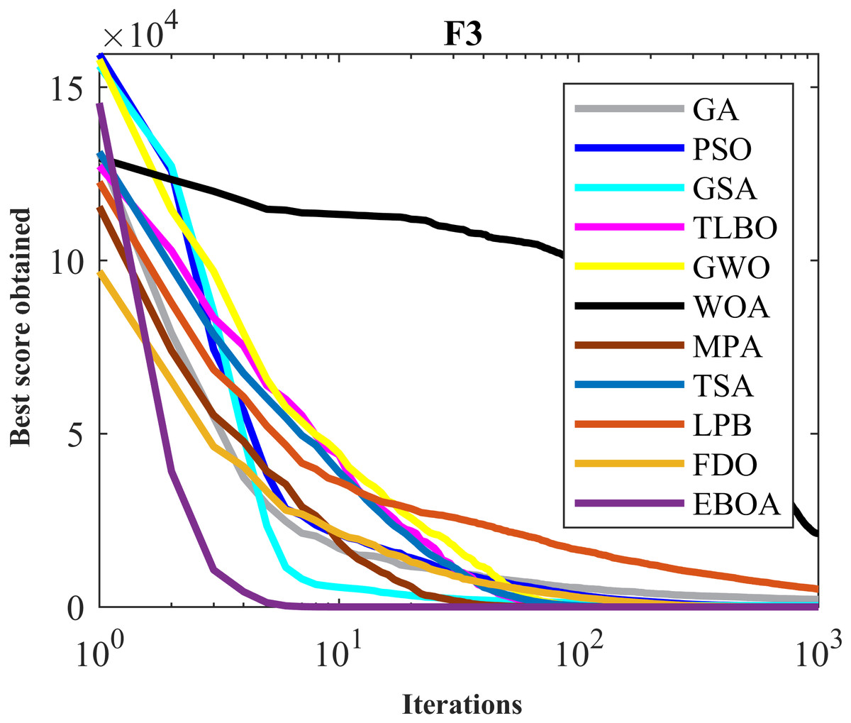
Figure 4: Convergence curves of EPOA and competitor algorithms on F3.
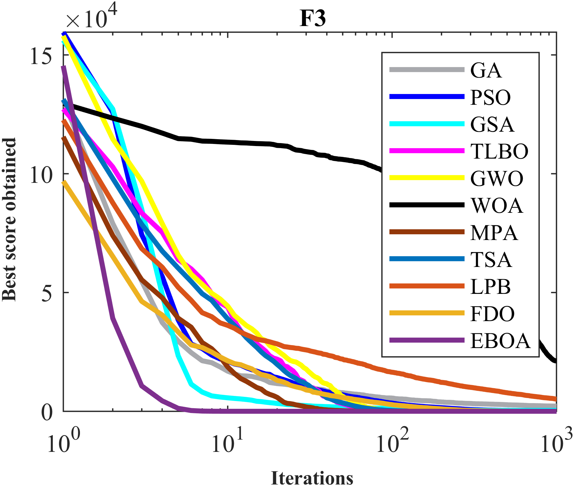
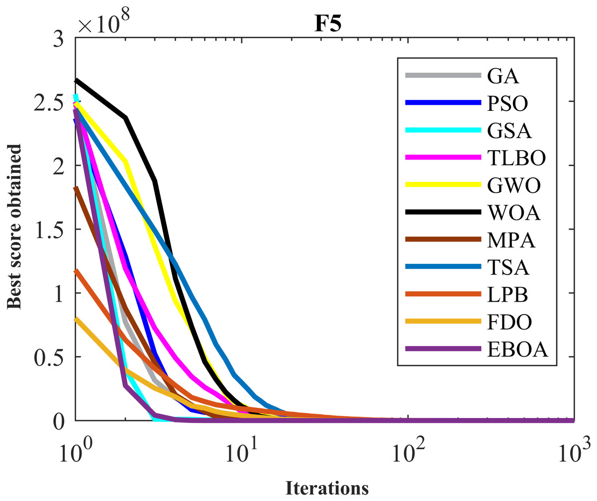
Figure 5: Convergence curves of EPOA and competitor algorithms on F5.
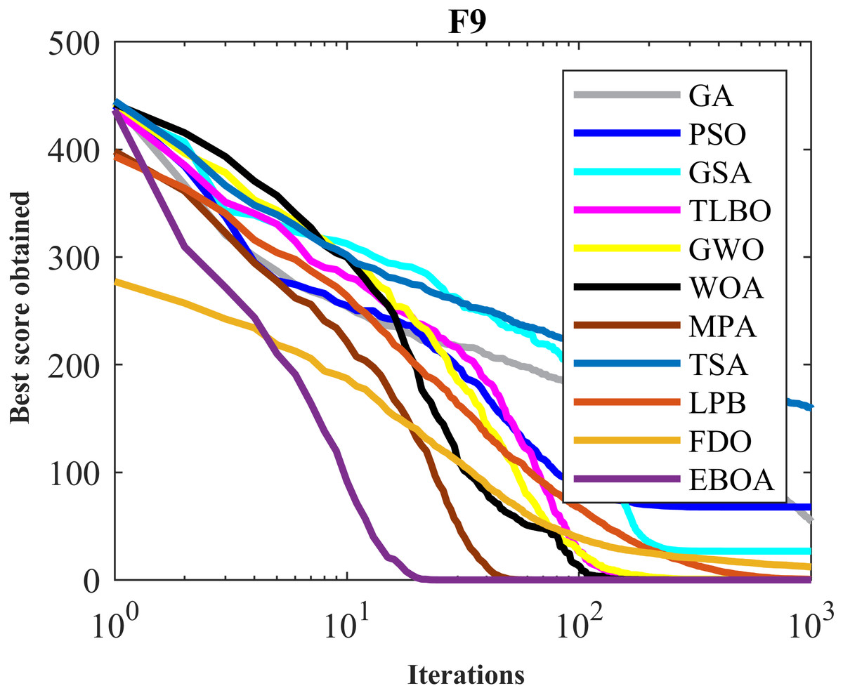
Figure 6: Convergence curves of EPOA and competitor algorithms on F9.
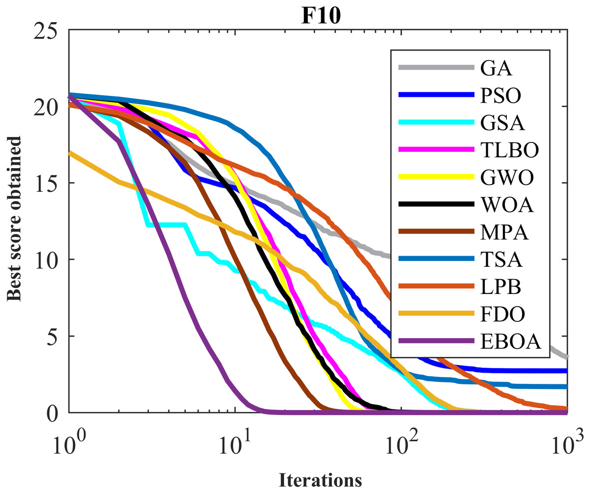
Figure 7: Convergence curves of EPOA and competitor algorithms on F10.
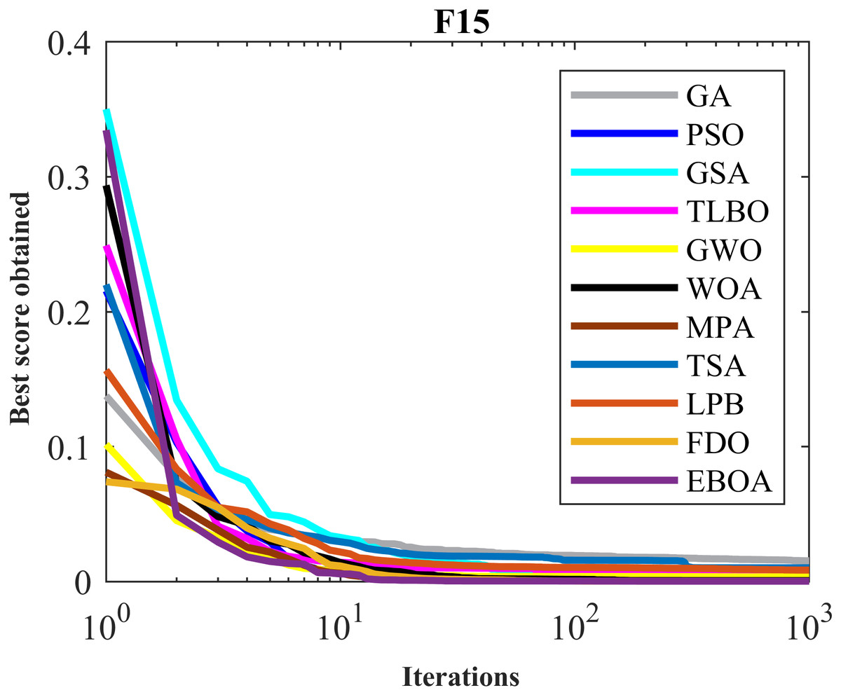
Figure 8: Convergence curves of EPOA and competitor algorithms on F15.
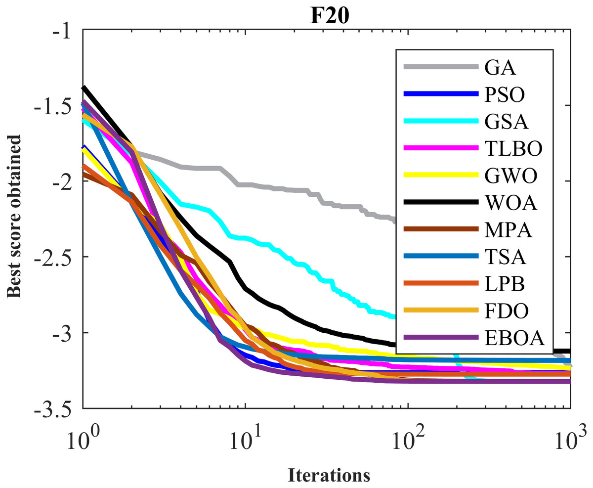
Figure 9: Convergence curves of EPOA and competitor algorithms on F20.
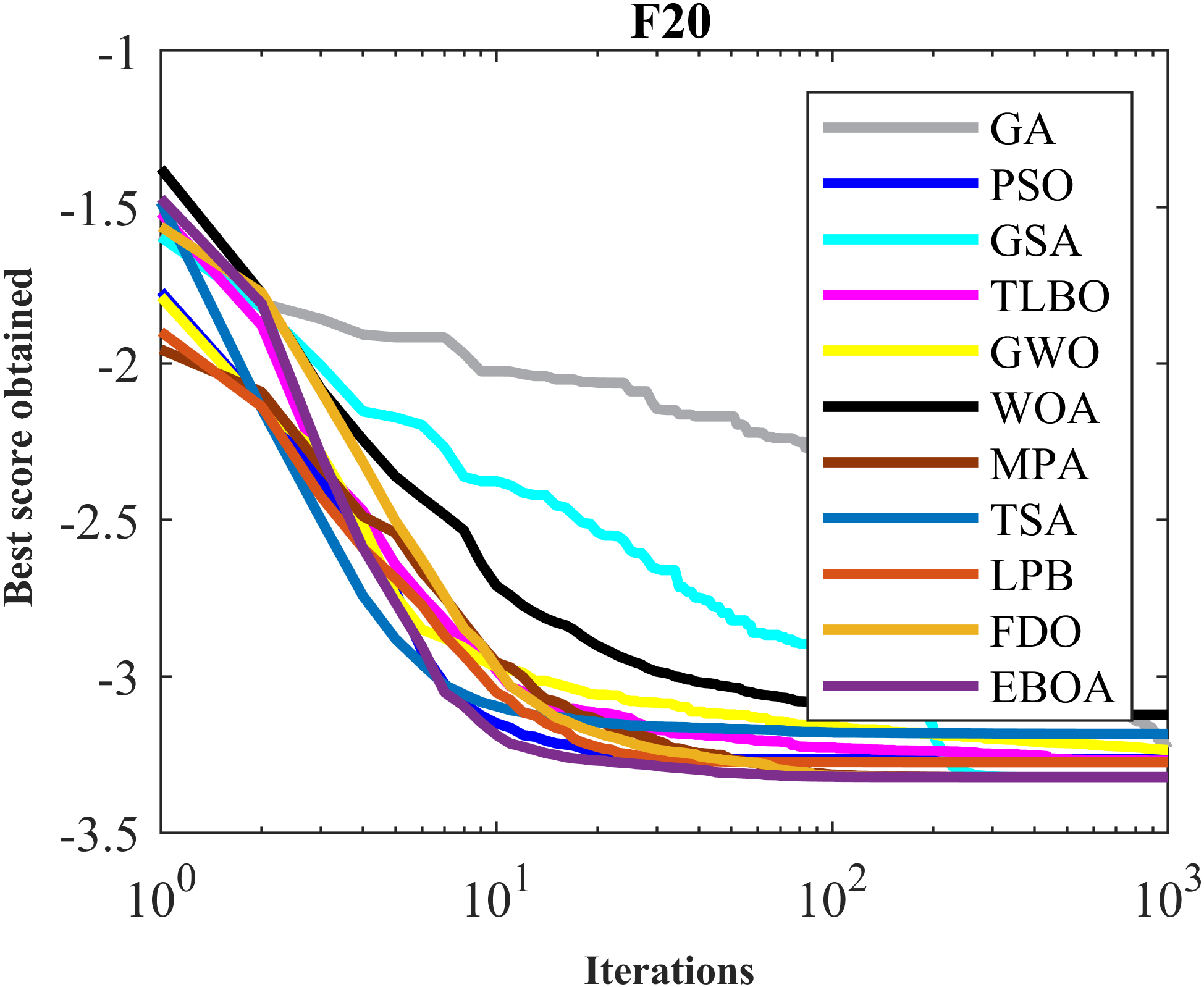
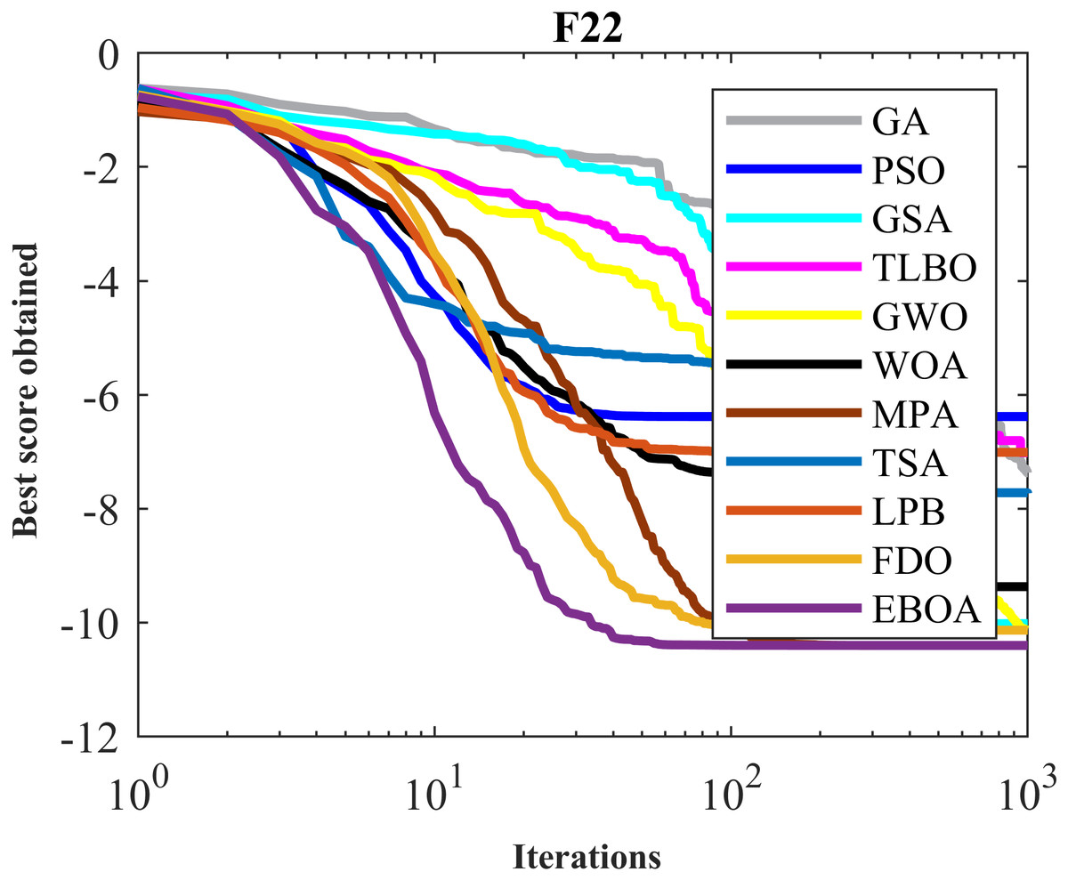
Figure 10: Convergence curves of EPOA and competitor algorithms on F22.

Figure 11: Convergence curves of EPOA and competitor algorithms on F23.
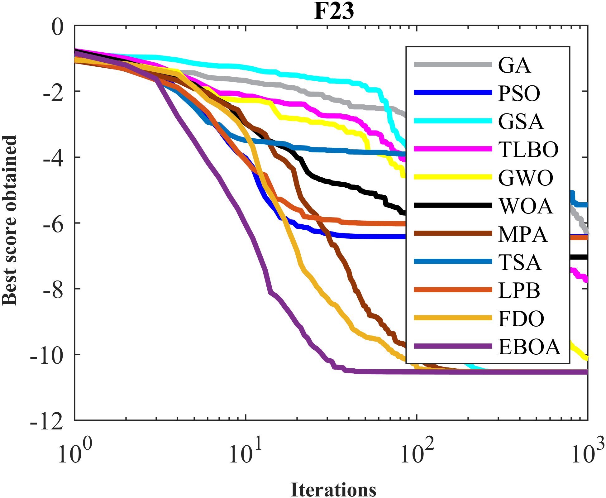
Statistical analysis
Capability analysis of metaheuristic algorithms in terms of mean, best, std, median, and rank indices provides valuable information to compare their performance. However, a very small probability can be considered for the chance superiority of one method over another. In this study, the Wilcoxon rank sum test (Wilcoxon, 1992) and non-parametric t-test (Kim, 2015) are used to determine whether the superiority of the EBOA over any of the competing metaheuristic algorithms was statistically significant. The results of applying Wilcoxon rank sum test and non-parametric t-test on EBOA performance and competitor metaheuristic algorithms are released in Tables 9 and 10, respectively. In cases where the p-value is less than 0.05, it can be concluded that there is a significant difference between the two compared groups. What is clear from the results of the Wilcoxon rank sum test and non-parametric t-test is that the EBOA has a significant superiority in terms of statistical analysis over all ten competing algorithms in all objective function groups.
Sensitivity analysis
The proposed EBOA approach is a population-based metaheuristic algorithm that addresses optimization problems in a repetitive-based process. Thus, the two parameters of EBOA, population number (N) and the maximum number of iterations of the algorithm (T), affect EBOA performance. This subsection is dedicated to the sensitivity analysis of EBOA to changes in N and T parameters.
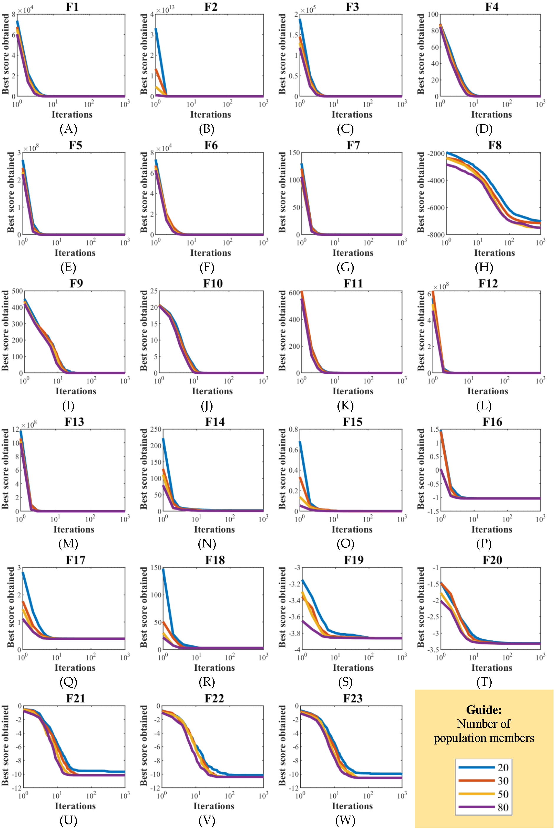
EBOA sensitivity analysis to parameter N has been studied by applying it to the handling of functions F1 to F23 for different values of parameter N equal to 20, 30, 50, and 80. The results of EBOA sensitivity analysis to parameter N are released in Table 11. The effect of the parameter N changes on EBOA convergence curves and how to achieve the solution is shown in Fig. 12. The simulation results reveal the fact that increasing the EBOA population size increases the search power of this algorithm, as it can be seen that by increasing the values of parameter N, the proposed EBOA achieves better solutions and as a result, the values of all objective functions decrease.
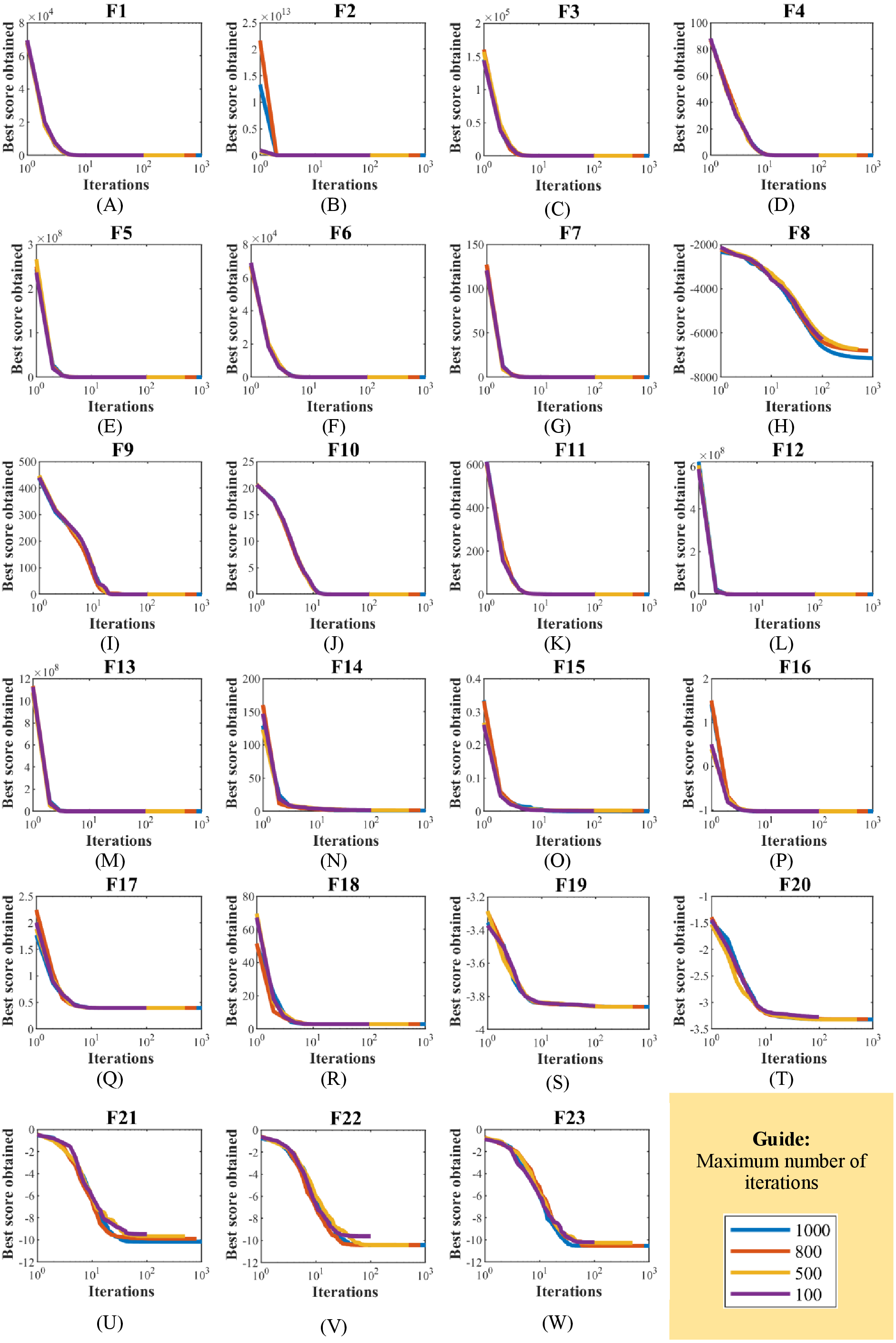
EBOA sensitivity analysis to the parameter T has been tested by implementing it on the handling of F1 to F23 functions for the parameter T equal to 100, 500, 800, and 1,000. The outputs of the EBOA sensitivity analysis for the T parameter value are shown in Table 12. In addition, the EBOA convergence curves, which show how to achieve the optimal solution under changes in the T parameter, are shown in Fig. 13. What can be understood from the simulation results is that increasing the number of iterations gives the EBOA more opportunity to be able to identify the main optimal area more accurately and to converge more towards the global optimal, which this reduced the values of the objective functions.
Evaluation of CEC 2019 suite objective functions
The implementation of EBOA on the functions F1 to F23 indicated the high ability of EBOA in optimization applications. In this subsection, the performance of the EBOA is evaluated in addressing the CEC 2019 objective functions, which consist of ten functions of CEC01 to CEC10. The optimization results of CEC 2019 functions using EBOA and competitor algorithms are presented in Table 13. EBOA is the first best optimizer in addressing the functions cec02, cec03, cec07, cec08, cec09, and cec10. The results of the Wilcoxon rank-sum test and t-test are reported in Table 14. In cases where the p-value in this table is less than 0.05, the proposed EBOA approach has a statistically significant superiority over the corresponding algorithm. Analysis of the simulation results shows that the proposed EBOA approach has a superior performance over competitor algorithms in handling most cases of CEC 2019 test functions.
Discussion
Exploitation and exploration are very influential on the performance of metaheuristic algorithms in finding optimal solutions to problems. Exploitation is the notion of local search capability around existing solutions that enables the algorithm to converge to better solutions that may be located in situations close to existing solutions. The impact of exploitation on the ability of metaheuristic algorithms is especially evident in dealing with problems that have only one main peak. The results of optimizing the functions F1 to F7 (with only the main peak) show that the EBOA has the high exploitation ability in local search and convergence to the global optimal solution. The high exploitation of the EBOA is especially evident in the handling of the functions F1, F3, and F6, which has converged to the global optimal.
Exploration is the concept of global search capability in all areas of the problem-solving space that enables the algorithm to identify the main optimal area containing the global optimal in the presence of local optimal areas. The effect of exploration on the ability of metaheuristic algorithms is especially evident in handling problems that have several non-optimal peaks in addition to the main peak. The results of optimizing the F8 to F13 functions (with several non-optimal peaks) show that the EBOA has acceptable exploration power in the global search and identification of the main optimal area. The high exploration capability of EBOA, especially in handling F9 and F11, has led to the accurate identification of the main optimal area and the success of the algorithm in achieving the global optimum.
| Compared algorithm | Objective function type | ||
|---|---|---|---|
| Unimodal | High-dimensional multimodal | Fixed-dimensional multimodal | |
| EBOA vs. GA | 1.01E−24 | 4.02E−18 | 1.04E−22 |
| EBOA vs. PSO | 1.01E−24 | 2.42E−20 | 3.74E−34 |
| EBOA vs. GSA | 9.78E−25 | 1.89E−21 | 1.28E−32 |
| EBOA vs. TLBO | 9.3E−21 | 3.51E−12 | 4.35E−33 |
| EBOA vs. GWO | 6.49E−23 | 6.96E−08 | 1.46E−24 |
| EBOA vs. WOA | 1.07E−13 | 4.58E−11 | 0.018214 |
| EBOA vs. TSA | 1.78E−20 | 2.37E−12 | 0.044185 |
| EBOA vs. MPA | 1.01E−24 | 5.53E−06 | 1.44E−34 |
| EBOA vs. LPB | 1.35E−21 | 0.0002 | 7.37E−31 |
| EBOA vs. FDO | 6.98E−12 | 6.05E−07 | 6.24E−15 |
| Compared algorithm | Objective function type | ||
|---|---|---|---|
| Unimodal | High-dimensional multimodal | Fixed-dimensional multimodal | |
| EBOA vs. GA | 0.018107 | 0.019062 | 0.034177 |
| EBOA vs. PSO | 6.78E−06 | 4.4E−06 | 1.45E−09 |
| EBOA vs. GSA | 1.25E−06 | 2.9E−06 | 0.015419 |
| EBOA vs. TLBO | 5.47E−06 | 3.01E−05 | 2.5E−13 |
| EBOA vs. GWO | 1.61E−06 | 4.42E−06 | 1.17E−11 |
| EBOA vs. WOA | 7.43E−06 | 0.00133 | 0.001565 |
| EBOA vs. TSA | 4.73E−06 | 0.031683 | 1.12E−10 |
| EBOA vs. MPA | 9.96E−06 | 5.93E−06 | 2.5E−07 |
| EBOA vs. LPB | 0.024004 | 0.075963 | 4.85E−11 |
| EBOA vs. FDO | 6.64E−08 | 0.001498 | 9.29E−13 |
| Objective functions | Number of population members | |||
|---|---|---|---|---|
| 20 | 30 | 50 | 80 | |
| F1 | 0 | 0 | 0 | 0 |
| F2 | 2.4E−210 | 1.3E−261 | 1.2E−291 | 0 |
| F3 | 0 | 0 | 0 | 0 |
| F4 | 4.2E−214 | 5.3E−260 | 1.1E−284 | 3.4E−304 |
| F5 | 26.39773 | 25.91771 | 25.51165 | 24.81 |
| F6 | 0 | 0 | 0 | 0 |
| F7 | 6.73E−05 | 4.77E−05 | 3.04E−05 | 1.99E−05 |
| F8 | −7006.16 | −7149.45 | −7477.15 | −7491.36 |
| F9 | 0 | 0 | 0 | 0 |
| F10 | 2.49E−15 | 1.24E−15 | 8.88E−16 | 8.88E−16 |
| F11 | 0 | 0 | 0 | 0 |
| F12 | 4.4E−07 | 2.71E−07 | 1.77E−07 | 1.1E−07 |
| F13 | 0.001125 | 3.88E−06 | 2.87E−06 | 1.6E−06 |
| F14 | 2.432658 | 0.998 | 0.998 | 0.998 |
| F15 | 0.000379 | 0.000308 | 0.000307 | 0.000307 |
| F16 | −1.03163 | −1.03163 | −1.03163 | −1.03163 |
| F17 | 0.397887 | 0.397887 | 0.397887 | 0.397887 |
| F18 | 3 | 3 | 3 | 3 |
| F19 | −3.86278 | −3.86278 | −3.86278 | −3.86278 |
| F20 | −3.31004 | −3.322 | −3.322 | −3.322 |
| F21 | −9.64339 | −10.1532 | −10.1532 | −10.1532 |
| F22 | −10.1371 | −10.4029 | −10.4029 | −10.4029 |
| F23 | −9.98805 | −10.5364 | −10.5364 | −10.5364 |
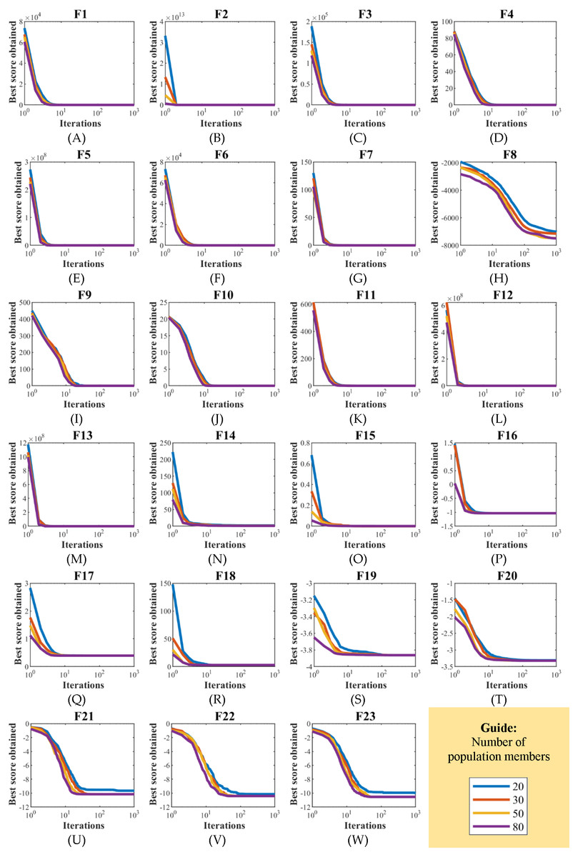
Figure 12: (A–T) EBOA convergence curves in the study of sensitivity analysis to population size N changes.
| Objective functions | Maximum number of iterations | |||
|---|---|---|---|---|
| 100 | 500 | 800 | 1,000 | |
| F1 | 3.52E−47 | 4.5E−263 | 0 | 0 |
| F2 | 1.09E−22 | 1.4E−125 | 8.9E−209 | 1.3E−261 |
| F3 | 1.08E−41 | 3.3E−231 | 0 | 0 |
| F4 | 9.21E−24 | 2.6E−127 | 3.9E−206 | 5.3E−260 |
| F5 | 28.41803 | 27.17727 | 26.53139 | 25.91771 |
| F6 | 0 | 0 | 0 | 0 |
| F7 | 0.000665 | 9.19E−05 | 5.67E−05 | 4.77E−05 |
| F8 | −6297.42 | −6741.15 | −6801.7 | −7149.45 |
| F9 | 0 | 0 | 0 | 0 |
| F10 | 2.15E−15 | 2.14E−15 | 2.13E−15 | 1.24E−15 |
| F11 | 0 | 0 | 0 | 0 |
| F12 | 0.001396 | 2.55E−06 | 1.02E−06 | 2.71E−07 |
| F13 | 0.068494 | 2.27E−05 | 2.04E−05 | 3.88E−06 |
| F14 | 0.998 | 0.998 | 0.998 | 0.998 |
| F15 | 0.000924 | 0.002341 | 0.001376 | 0.000308 |
| F16 | −1.03163 | −1.03163 | −1.03163 | −1.03163 |
| F17 | 0.397889 | 0.397887 | 0.397887 | 0.397887 |
| F18 | 3 | 3 | 3 | 3 |
| F19 | −3.8582 | −3.86278 | −3.86278 | −3.86278 |
| F20 | −3.27088 | −3.29773 | −3.30403 | −3.322 |
| F21 | −9.47147 | −9.53358 | −9.64336 | −10.1532 |
| F22 | −9.60492 | −10.4029 | −10.4029 | −10.4029 |
| F23 | −10.2011 | −10.4668 | −10.5364 | −10.5364 |
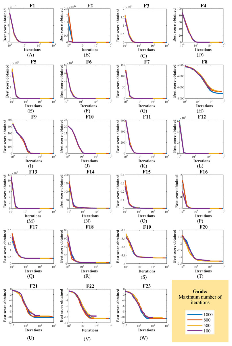
Figure 13: (A–W) EBOA convergence curves in the study of sensitivity analysis to maximum number of iterations T changes.
In addition to having high capabilities in exploration and exploitation, the conditions that predispose metaheuristic algorithms to success in achieving solutions are the proper balance between these two indicators. Objective functions F14 to F23 have fewer non-optimal peaks than functions F8 to F13, and are good criteria for analyzing the ability of optimization algorithms to have the proper balance between exploration and exploitation. The results of optimization of F14 to F23 functions indicate that EBOA has a high potential for balancing exploration and exploitation to identify the main optimal region and converge towards the global optimal. An overall analysis of the results of optimizing the F1 to F23 objective functions frees the inference that the proposed EBOA approach has a high potential for exploration and exploitation as well as a balance between the two capabilities.
Conclusions
Metaheuristic algorithms are one of the most widely used and effective stochastic methods for solving optimization problems. In this study, a new human-based algorithm called the Election Based Optimization Algorithm (EBOA) was proposed. The fundamental inspiration of the EBOA is the voting and election process in which people vote for their preferred candidate to elect the leader of the population. The EBOA steps in two phases of (i) exploration, including election holding and (ii) exploitation, including raising public awareness for better decision-making are mathematically modeled. The efficiency of EBOA in providing solutions to optimization problems was tested on thirty-three standard benchmark functions of a variety of unimodal, high-dimensional multimodal, fixed-dimensional multimodal, CEC 2019 types. The optimization results of unimodal functions indicated the high exploitation ability of EBOA in local search. The optimization results of high-dimensional multimodal functions showed the EBOA exploration capability in the global search of problem-solving space. In addition, the results obtained from the optimization of fixed-dimensional multimodal functions concluded that EBOA, by creating the proper balance between exploration and exploitation, has an effective efficiency in providing solutions to this type of problems. The implementation of EBOA on the complex CEC2019 suite test functions indicated the effectiveness of the proposed approach in dealing with complex optimization problems. The quality of the results delivered by the EBOA is compared against the performance of ten state-of-the-art metaheuristic algorithms. Comparing the simulation results, it can be found that EBOA has provided better optimization results and is much more competitive than the ten metaheuristic algorithms. The findings of simulation, statistical analysis, and sensitivity analysis indicate the high capability and efficiency of the EBOA in dealing with optimization issues.
| EBOA | FDO | LPB | MPA | TSA | WOA | GWO | TLBO | GSA | PSO | GA | ||
|---|---|---|---|---|---|---|---|---|---|---|---|---|
| cec01 | Mean | 31397.63 | 15232289 | 2.89E+10 | 31395.7 | 1.65E+08 | 2.12E+10 | 79199216 | 4.33E+08 | 3.24E+12 | 4.6E+08 | 5.52E+10 |
| Best | 31395.7 | 187157.2 | 1.57E+09 | 31395.7 | 39799.58 | 1773823 | 45782.62 | 101859.5 | 6.80E+11 | 4374858 | 6.23E+09 | |
| std | 5.282375 | 22511868 | 2.09E+10 | 0.000292 | 4.16E+08 | 2.76E+10 | 1.1E+08 | 7.95E+08 | 2.05E+12 | 1.36E+09 | 4.6E+10 | |
| Median | 31395.79 | 4646710 | 2.52E+10 | 31395.7 | 2266337 | 8.34E+09 | 35900762 | 1.01E+08 | 2.94E+12 | 69939138 | 4.1E+10 | |
| Rank | 2 | 3 | 9 | 1 | 5 | 8 | 4 | 6 | 11 | 7 | 10 | |
| cec02 | mean | 17.34286 | 17.34286 | 27.70728 | 17.34286 | 18.34769 | 17.34508 | 17.34332 | 17.37083 | 14774.91 | 17.34286 | 53.56418 |
| Best | 17.34286 | 17.34286 | 17.34892 | 17.34286 | 17.34803 | 17.34302 | 17.34311 | 17.35692 | 7679.092 | 17.34286 | 19.23928 | |
| std | 0 | 2.61E−09 | 13.66182 | 7.89E−12 | 0.808127 | 0.001867 | 0.000124 | 0.008292 | 4550.232 | 3.05E−15 | 31.00016 | |
| Median | 17.34286 | 17.34286 | 21.74086 | 17.34286 | 18.17572 | 17.34464 | 17.3433 | 17.36932 | 14635.08 | 17.34286 | 41.51365 | |
| Rank | 1 | 4 | 9 | 3 | 8 | 6 | 5 | 7 | 11 | 2 | 10 | |
| cec03 | mean | 12.7024 | 12.7024 | 12.7024 | 12.7024 | 12.70296 | 12.7024 | 12.7025 | 12.70241 | 12.7024 | 12.7024 | 12.70241 |
| Best | 12.7024 | 12.7024 | 12.7024 | 12.7024 | 12.7024 | 12.7024 | 12.7024 | 12.70241 | 12.7024 | 12.7024 | 12.7024 | |
| std | 3.65E−15 | 1.50E−11 | 5.55E−08 | 3.65E−15 | 0.001339 | 5.24E−07 | 0.000415 | 9.08E−06 | 3.65E−15 | 2.08E−15 | 1.85E−06 | |
| Median | 12.7024 | 12.7024 | 12.7024 | 12.7024 | 12.70247 | 12.7024 | 12.7024 | 12.70241 | 12.7024 | 12.7024 | 12.7024 | |
| Rank | 1 | 3 | 4 | 1 | 9 | 5 | 8 | 7 | 1 | 2 | 6 | |
| cec04 | mean | 29.40091 | 25.8849 | 79.20654 | 8.011005 | 4244.962 | 253.3125 | 264.7791 | 230.9865 | 6.51698 | 67.58687 | 134.1774 |
| Best | 12.93446 | 7.960353 | 20.97703 | 0.00017 | 74.23499 | 110.3315 | 13.37336 | 161.5526 | 2.984877 | 10.94454 | 38.25033 | |
| std | 14.08728 | 8.968979 | 47.08096 | 4.384481 | 2404.606 | 154.3524 | 581.9962 | 52.66575 | 2.247511 | 116.2151 | 59.15384 | |
| Median | 26.36631 | 25.30171 | 70.53092 | 8.470501 | 4468.768 | 215.8693 | 57.17001 | 225.0158 | 6.964711 | 29.8487 | 135.3556 | |
| Rank | 4 | 3 | 6 | 2 | 11 | 9 | 10 | 8 | 1 | 5 | 7 | |
| cec05 | mean | 1.160508 | 1.111998 | 1.226455 | 1.050818 | 2.999024 | 1.576271 | 1.266711 | 1.857917 | 1.00948 | 1.193098 | 1.602569 |
| Best | 1.051728 | 1.040138 | 1.048986 | 1.014772 | 1.871421 | 1.201734 | 1.058202 | 1.658814 | 1 | 1.063978 | 1.288733 | |
| std | 0.065115 | 0.038701 | 0.133284 | 0.032407 | 1.072619 | 0.251901 | 0.208595 | 0.138394 | 0.010012 | 0.208163 | 0.214074 | |
| Median | 1.137767 | 1.121755 | 1.193437 | 1.044283 | 2.632057 | 1.576226 | 1.189335 | 1.8488 | 1.007396 | 1.145125 | 1.552622 | |
| Rank | 4 | 3 | 6 | 2 | 11 | 8 | 7 | 10 | 1 | 5 | 9 | |
| cec06 | mean | 2.106428 | 8.140997 | 5.623278 | 1.818019 | 10.42986 | 8.978288 | 10.42138 | 10.59729 | 1.000105 | 3.993241 | 8.647723 |
| Best | 1.15137 | 5.874072 | 4.320987 | 1.114883 | 9.163213 | 7.276666 | 9.009652 | 9.853189 | 1.000073 | 1.228136 | 5.785451 | |
| std | 0.660714 | 0.661779 | 0.807592 | 0.744312 | 0.692189 | 1.124288 | 0.783399 | 0.434776 | 1.97E−05 | 1.907946 | 1.341339 | |
| Median | 1.929794 | 8.217592 | 5.516918 | 1.404095 | 10.3353 | 8.741017 | 10.26319 | 10.6044 | 1.000105 | 4.0335 | 9.229273 | |
| Rank | 3 | 6 | 5 | 2 | 10 | 8 | 9 | 11 | 1 | 4 | 7 | |
| cec07 | mean | 112.4807 | 143.7672 | 237.0939 | 174.3536 | 617.3397 | 616.2879 | 418.7292 | 623.5747 | 187.8737 | 165.1417 | 124.3327 |
| Best | 14.75369 | 90.65738 | 61.10223 | 110.9085 | 246.6122 | 148.1279 | 79.03335 | 304.7375 | 82.15282 | 10.37837 | 12.09356 | |
| std | 79.22918 | 32.18216 | 140.8724 | 45.33848 | 259.8789 | 349.1442 | 300.5297 | 178.8176 | 90.5322 | 132.6008 | 92.31307 | |
| Median | 112.4599 | 144.3338 | 215.906 | 152.9829 | 597.9233 | 632.1518 | 334.0758 | 603.1046 | 180.2679 | 148.4302 | 120.9174 | |
| Rank | 1 | 3 | 7 | 5 | 10 | 9 | 8 | 11 | 6 | 4 | 2 | |
| cec08 | mean | 2.546949 | 4.300242 | 5.419414 | 3.869595 | 6.139661 | 5.839999 | 4.761854 | 5.360152 | 5.372261 | 5.021396 | 5.04118 |
| Best | 1.289734 | 3.083263 | 3.559119 | 2.708939 | 4.895428 | 4.841095 | 2.925632 | 4.301028 | 4.363495 | 3.633744 | 4.04053 | |
| std | 0.727627 | 0.610021 | 0.598187 | 0.616791 | 0.472164 | 0.523359 | 0.942676 | 0.737183 | 0.499415 | 0.644997 | 0.466454 | |
| Median | 2.703282 | 4.336097 | 5.419597 | 4.034933 | 6.234195 | 5.892174 | 4.984088 | 5.222119 | 5.35066 | 5.112039 | 5.042585 | |
| Rank | 1 | 3 | 9 | 2 | 11 | 10 | 4 | 7 | 8 | 5 | 6 | |
| cec09 | mean | 2.343608 | 2.367272 | 3.13243 | 2.359083 | 440.234 | 4.575637 | 4.416888 | 19.60514 | 3.14272 | 2.549543 | 3.668416 |
| Best | 2.33839 | 2.346984 | 2.720081 | 2.341292 | 2.896331 | 3.582951 | 3.596261 | 4.652537 | 2.576973 | 2.395394 | 2.819678 | |
| std | 0.005293 | 0.015551 | 0.288009 | 0.022234 | 591.7603 | 0.891569 | 0.651956 | 61.46722 | 0.494874 | 0.131925 | 0.509679 | |
| Median | 2.341382 | 2.362613 | 3.144558 | 2.35069 | 279.8453 | 4.582947 | 4.431976 | 5.863226 | 3.011512 | 2.514102 | 3.538552 | |
| Rank | 1 | 3 | 5 | 2 | 11 | 9 | 8 | 10 | 6 | 4 | 7 | |
| cec10 | mean | 5.313416 | 20.00304 | 20.03576 | 17.11663 | 20.4158 | 20.16707 | 20.43476 | 19.50824 | 18.64584 | 20.00118 | 19.3639 |
| Best | 8.88E−16 | 19.91337 | 20.01024 | 0.000229 | 20.26639 | 20.04477 | 20.29121 | 9.348959 | 3.25E−09 | 19.99751 | 7.534284 | |
| std | 8.723522 | 0.041617 | 0.019828 | 7.057655 | 0.069939 | 0.102794 | 0.082589 | 2.869468 | 4.639721 | 0.006276 | 3.0762 | |
| Median | 1.15E−14 | 19.99981 | 20.03535 | 20 | 20.40561 | 20.14991 | 20.44391 | 20.38098 | 19.99088 | 19.99974 | 20.24951 | |
| Rank | 1 | 7 | 8 | 2 | 10 | 9 | 11 | 5 | 3 | 6 | 4 | |
| Sum rank | 19 | 38 | 68 | 22 | 96 | 81 | 74 | 82 | 49 | 44 | 68 | |
| Mean rank | 1.9 | 3.8 | 6.8 | 2.2 | 9.6 | 8.1 | 7.4 | 8.2 | 4.9 | 4.4 | 6.8 | |
| Total rank | 1 | 3 | 5 | 2 | 10 | 8 | 7 | 9 | 5 | 4 | 6 | |
| Compared algorithm | Test type | |
|---|---|---|
| Wilcoxon rank sum test | t-test | |
| EBOA vs. GA | 1.21E−23 | 0.000446 |
| EBOA vs. PSO | 1.4E−12 | 0.14247 |
| EBOA vs. GSA | 1.01E−08 | 0.000112 |
| EBOA vs. TLBO | 9.19E−34 | 0.028878 |
| EBOA vs. GWO | 5.17E−26 | 0.007451 |
| EBOA vs. WOA | 2.66E−34 | 0.005366 |
| EBOA vs. TSA | 1.44E−34 | 0.09192 |
| EBOA vs. MPA | 0.244915 | 0.048768 |
| EBOA vs. LPB | 3.89E−27 | 0.000215 |
| EBOA vs. FDO | 4.12E−16 | 0.010523 |
The proposed EBOA approach enables several future directions, the most specific of which are the development of the EBOA binary version for discrete space applications, and the design of the EBOA multi-objective version to handle multi-objective optimization problems. The EBOA is applied to solve optimization problems in various sciences as well as real-world applications are other suggestions for future directions.
The proposed EBOA approach is a stochastic-based solving method. So, the main limitation of EBOA, similar to all stochastic-based approaches, is there is no guarantee that EBOA will achieve the optimal global solution. In addition, EBOA may fail to address some optimization applications because, according to the NFL theorem, there is no presumption that a metaheuristic algorithm is successful or not. Another limitation of EBOA is that it is always possible to develop newer algorithms that perform better than existing algorithms and EBOA. However, the optimization results show that the EBOA has provided solutions that are very close to the global optimal and, in some cases, precisely the global optimal. This EBOA capability is particularly evident in optimizing the F1, F3, F6, F9, F11, and F18 because it has made available the optimal global solution.
Supplemental Information
Matlab code of proposed algorithm EBOA
A proposed algorithm that implements EBOA steps on optimization of objective functions and publishes the optimal solution in the output.
File of code for objective functions
Determines the information of the objective function and provides it to the main program.
Input of the EBOA optimizer
The main implementation code that call the information of the objective functions (including: number of variables, upper and lower band of variables, and mathematical formula of the objective function). This code then puts the objective function information as the input of the EBOA optimizer to determine its optimal solution.