Structural mapping of oligomeric intermediates in an amyloid assembly pathway
- University of Leeds, United Kingdom
Figures
Figure 1
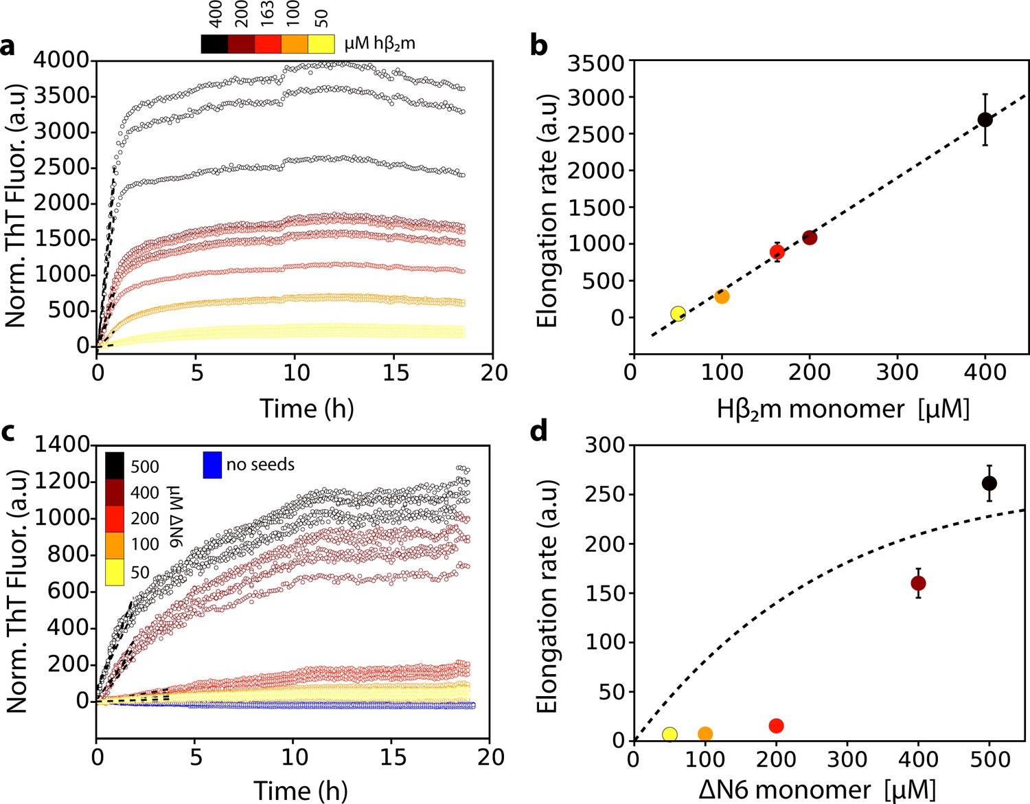
Dependence of the fibril elongation rate on the concentration of soluble protein.
Seeded elongation assays for (a) hβ2m at pH 2.0 monitored by ThT fluorescence. 20 μM of preformed seeds of hβ2m (formed at pH 2.0) and varying amounts of soluble protein were added, as indicated in the key. Note that the protein does not aggregate under these conditions in the absence of seeds on this timescale (Xue et al., 2008). The dashed line shows the initial rate of each reaction. (b) The initial rate of fibril elongation (shown in units of ThT fluorescence (a.u.)/h) versus the concentration of hβ2m added. The dashed line represents a prediction using a monomer addition model (see Table 4). (c) Seeded elongation assays for ΔN6 using 20 μM preformed seeds formed from ΔN6 at pH 6.2 as a function of the concentration of soluble ΔN6 added. Open blue symbols denote the ThT fluorescence signal of 500 μM ΔN6 in the absence of seeds. The dashed line shows the initial rate of each reaction. (d) The initial rate of fibril elongation (shown in units of ThT fluorescence (a.u)/h) versus the concentration of soluble ΔN6 added. The dashed line shows the dependence of the elongation rate (in units of ThT fluorescence (a.u)/h) on the concentration of monomer assuming a monomer addition model (see Table 4). The elongation rate for monomer addition shows a hyperbolic behavior as a function of monomer concentration, with a linear dependence at lower monomer concentrations, followed by a saturation phase at higher monomer concentrations. The simulation in (b) (dashed line) uses a slower microscopic elongation rate (ke) (Table 4) than that used in panel (d) and therefore saturation is not achieved by 410 μM protein in (b), but is in (d). Five replicates are shown for each protein concentration. Error bars show the standard deviation between all replicates.
Figure 2 with 2 supplements
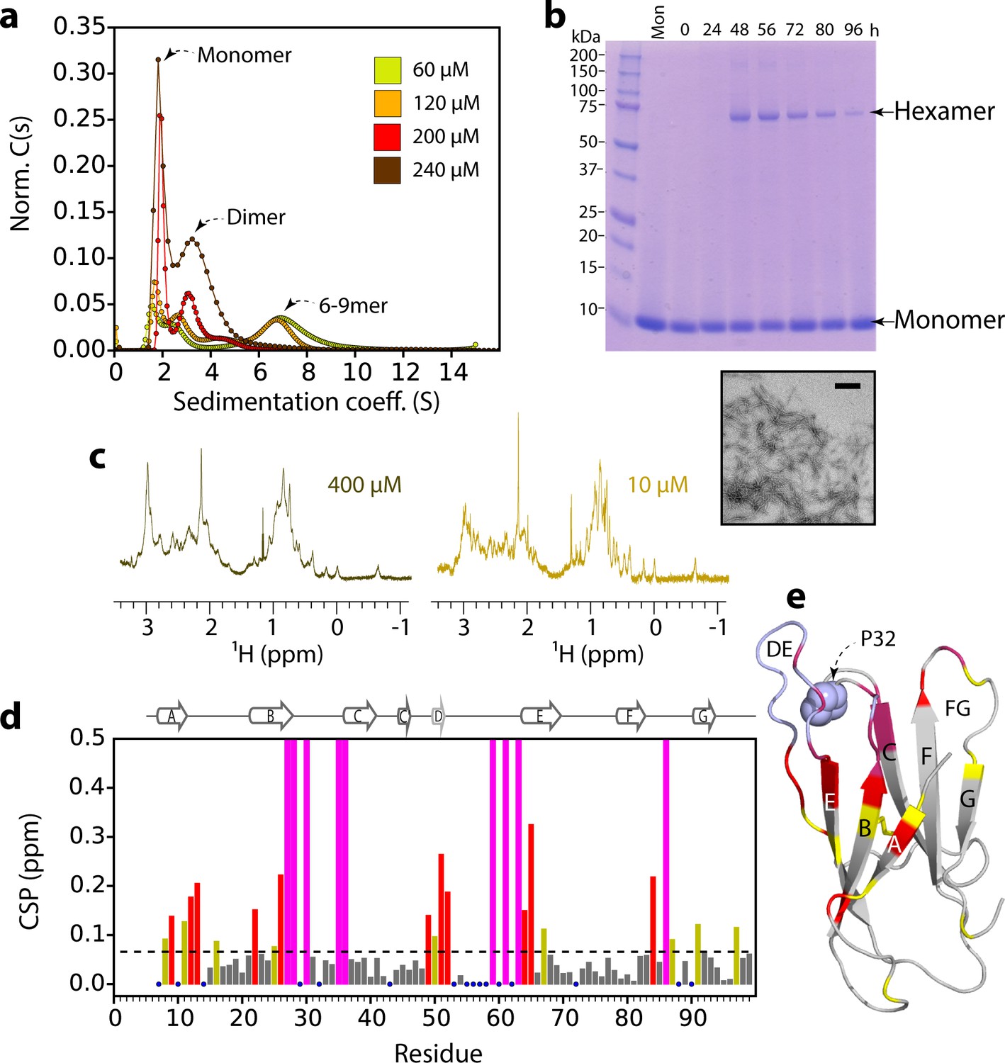
ΔN6 oligomer formation.
(a) Sedimentation velocity AUC of ΔN6 at different concentrations, as indicated by the key. Note that the higher order species decrease in intensity at high protein concentrations (>200 μM) consistent with the formation of large aggregates that sediment rapidly before detection (see also Figure 2—figure supplement 1d). (b) SDS–PAGE of cross-linked ΔN6 (80 μM) at different time-points during de novo fibril assembly in the absence of fibril seeds (see Materials and methods). Note that dimers are not observed, presumably as they are not resilient to the vigorous agitation conditions used to accelerate fibril formation in these unseeded reactions, or are not efficiently cross-linked by EDC under the conditions used (see Materials and methods). A negative stain electron micrograph of ΔN6 after 100 hr of incubation is shown below. Scale bar – 500 nm. (c) The methyl region of the 1H NMR spectrum of ΔN6 at 400 μM (left) or 10 μM ΔN6 (right). (d) Per residue combined 1H-15N chemical shift differences between the 1H-15N HSQC spectrum of ΔN6 at 10 μM and 400 μM. Blue dots represent residues for which assignments are missing in both spectra. The dashed line represents one standard deviation (σ) of chemical shifts across the entire dataset. Residues that show chemical shift differences > 1σ are shown in yellow,>2σ are colored red, and residues for which the chemical shift difference is not significant (<1σ) are colored gray. Residues that are broadened beyond detection in the spectrum obtained at 400 μM are colored in magenta (see also Figure 2—figure supplement 2a). Residues are numbered according to the sequence of the WT protein. Arg 97 is hydrogen bonded to residues in the N-terminus and presumably is indirectly affected by the interaction. (e) The structure of ΔN6 (2XKU; Eichner et al., 2011) colored in the same scheme as (d). Pro32 is shown in blue space-fill. The buffer used in all experiments was 10 mM sodium phosphate pH 6.2 containing 83.3 mM NaCl (to maintain a constant ionic strength of 100 mM for all experiments), 25°C.
Figure 2—figure supplement 1
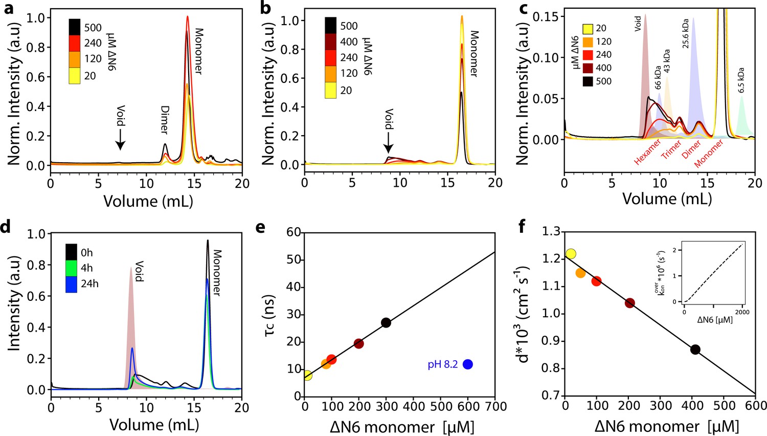
Analysis of ΔN6 oligomerization.
(a) Analytical SEC traces of uncross-linked ΔN6 at different concentrations as indicated in the key. (b) Analytical SEC traces of cross-linked ΔN6. (c) Zoom-in of the SEC traces shown in (b). The elution profile of protein standards is shaded in the background. (d) Analytical SEC traces of 500 μM ΔN6 0 hr (black), 4 hr (green) or 24 hr (blue) after cross-linking was performed. (e) Protein correlation times (τc) measured using a 1H-TRACT experiment (see Materials and methods) as a function of ΔN6 concentration at pH 6.2, colored as in (b). The black line represents a linear fit to the data. The correlation time of 600 μM ΔN6 at pH 8.2 is shown in blue. (f) The exponential decay rate (d) of the 1H NMR signal in a diffusion measurement using stimulated echoes as a function of ΔN6 concentration. The black line represents a linear fit to the data. The linear scaling of τc and d is predicted from the linear dependence of the overall assembly rate koveron on ΔN6 concentration using the calculated Kds and a monomer-dimer-hexamer model (inset) (see Materials and methods). Data points are colored as in (b). Error bars in (e) and (f) are calculated from the noise level of the spectra and are smaller than the marker points.
Figure 2—figure supplement 2
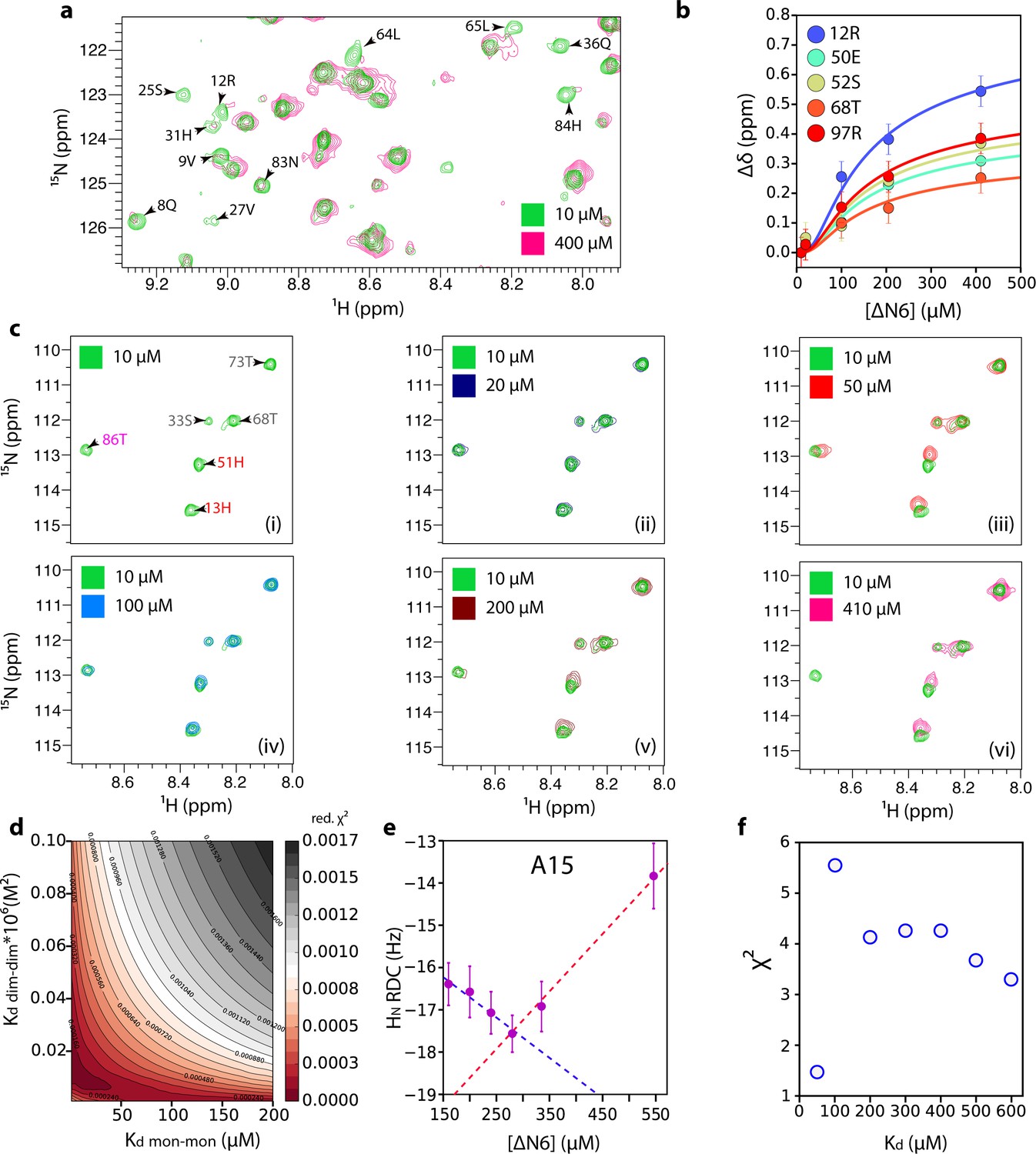
Estimation of dimer and hexamer Kd values.
(a) 1H-15N HSQC spectra of 10 μM (green) or 400 μM (pink) ΔN6. Resonances which are broadened >80% at 400 μM ΔN6 are indicated on the spectrum. (b) The combined 1H-15N chemical shift differences that report on hexamer formation as a function of ΔN6 concentration (the data at 50 μM are excluded since at this concentration the equilibrium is dominated by dimer formation). The solid lines represent fits to a monomer-dimer-hexamer model using a dimer Kd of 50 μM and a hexamer Kd of 10 × 10−9 M2 (see Materials and methods). Error bars represent the standard deviation of the resonances that do not show significant chemical shift changes between 10 and 410 μM ΔN6. Data were acquired at 25°C in 10 mM sodium phosphate pH 6.2 containing 83.3 mM NaCl (total ionic strength of 100 mM). (c) 1H-15N HSQC spectra of 10 μM (panel i), 20 μM (panel ii), 50 μM (panel iii), 100 μM (panel iv), 200 μM (panel v) or 410 μM (panel vi) ΔN6. Residues are labeled in panel (i) according to the color scheme of Figure 2d. (d) Reduced χ (Benilova et al., 2012) surface produced by fits to the monomer-dimer-hexamer model using the 10 residues (11, 12, 23, 26, 50, 51, 52, 67, 68, 97) that showed the largest chemical shift changes. (e) HN RDCs as a function of the ΔN6 concentration (a single example for A15 is shown for clarity). (f) Reduced χ (Benilova et al., 2012) values for the fitting of RDC data over the 41 residues measured to the structure of ΔN6 as a function of the Kd value used to extrapolate the RDCs to 100% dimer (see Materials and methods). Error bars were calculated from the noise level of the experiment.
Figure 3 with 2 supplements
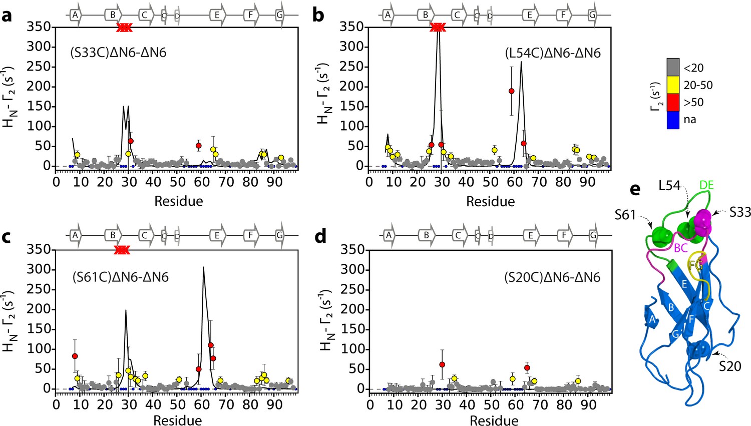
Identification of interacting surfaces in ΔN6 dimers.
Intermolecular PRE data for the self-association of ΔN6. 15N-ΔN6 (60 μM) was mixed with an equal concentration of (a) 14N-(S33C)ΔN6-MTSL; (b) 14N-(L54C)ΔN6-MTSL; (c) 14N-(S61C)ΔN6-MTSL; or (d) 14N-(S20C)ΔN6-MTSL in 10 mM sodium phosphate buffer, pH 6.2 containing 83.3 mM NaCl (a total ionic strength of 100 mM). The resulting Γ2 rates are color-coded according to the amplitude of the PRE effect (see scale bar: gray-insignificant (<20 s−1), yellow->20 s−1, red->50 s−1, pH 6.2, 25°C). Blue dots in the plots are residues for which resonances are not assigned (na) at pH 6.2. Red crosses indicate high HN-Γ2 rates for which an accurate value could not be determined. Control experiments showed that the small PREs arising from14N-(S20C)ΔN6-MTSL arise from non-specific interactions with MTSL itself. Solid black lines depict fits to the PRE data for the dimer structure shown in Figure 4a. Note the poor fits for some residues which are sensitive to hexamer formation (14% of ΔN6 molecules) under the conditions used. Residues are numbered according to the WT sequence and the position of β-strands (2XKU; Eichner et al., 2011) is marked above each plot. (e) The structure of ΔN6 (2XKU; Eichner et al., 2011) with the BC loop shown in magenta, the DE loop in green and the FG loop in yellow. The MTSL attachment sites are highlighted as spheres.
Figure 3—figure supplement 1

Lack of a hexamer population precludes aggregation of ΔN6 at pH 8.2.
(a) Aggregation assays for 60 μM ΔN6 monitored by ThT fluorescence at pH 6.2 (red) or pH 8.2 (blue), 37°C with agitation (600 rpm). Five replicates are shown. Negative stain transmission electron micrographs of samples at 100 hr are shown alongside in the same color code. (b) Sedimentation velocity AUC traces for 120 μM ΔN6 at pH 6.2 (red) or pH 8.2 (blue). (c,d) Intermolecular PRE values for ΔN6 at pH 8.2. 60 μM 15N-ΔN6 was mixed with (c) 60 μM of 14N-(S61C)ΔN6-MTSL or (d) 60 μM of 14N-(S20C)ΔM6-MTSL in 10 mM sodium phosphate buffer, pH 8.2 containing 86.6 mM NaCl (total ionic strength 100 mM). Γ2 rates are color-coded according to their amplitude (blue-not assigned, gray-insignificant (<20 s−1), yellow->20 s-1, red->50 s−1 at pH 8.2, 25°C). Residues are numbered according to the WT sequence. The position of β-strands (from 2XKU; Eichner et al., 2011) is marked above each plot.
Figure 3—figure supplement 2
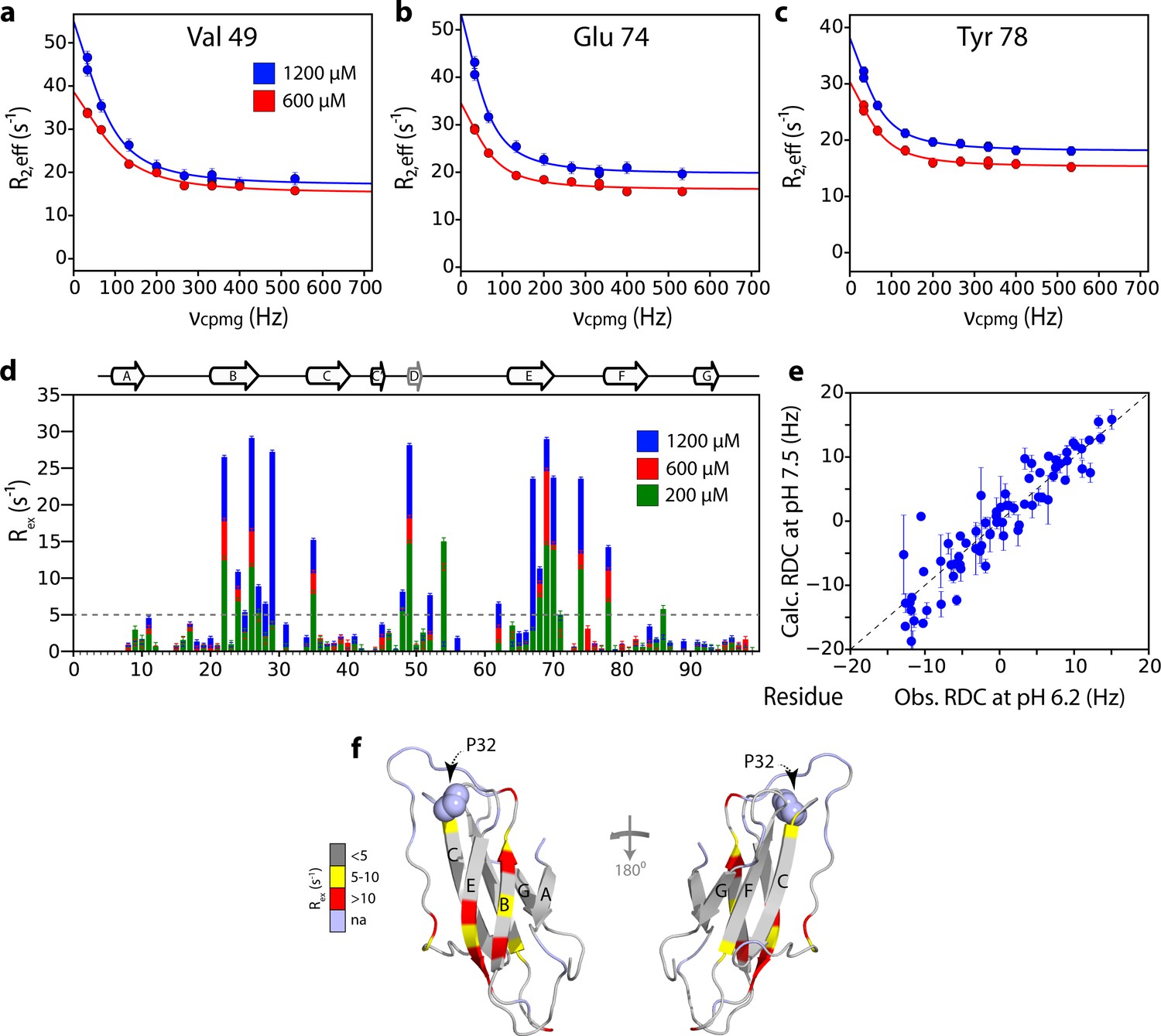
Mapping the interface of ΔN6 self-association at pH 8.2 using CPMG experiments.
15N Relaxation dispersion CPMG data for residues (a) V49, (b) E74 and (c) Y78 at 1200 μM (blue) or 600 μM ΔN6 (red). Solid lines represent fits to a fast exchange model (see Materials and methods). (d) Plots of Rex (defined as R2,eff50Hz - R2,eff680Hz) per residue at different concentrations of ΔN6 at pH 8.2 as indicated in the key. The dashed line represents one standard deviation of the mean. (e) Correlation plot of HN RDCs measured at pH 6.2 versus those back-calculated from the structure of ΔN6 (2XKU; Eichner et al., 2011; Eisenberg et al., 1984) at pH 7.5. (f) The structure of ΔN6 monomers (2XKU; Eichner et al., 2011) colored according the amplitude of the Rex values at 1200 μM shown in (d). The results show that the interface between interacting monomers at pH 8.2 involves interaction between β-sheets mediated by residues in the B, D and E β-strands and adjacent residues in the DE loop. This interface is very different to the loop-loop interactions that create the dimer interface at pH 6.2 (see Figure 3e).
Figure 4 with 1 supplement
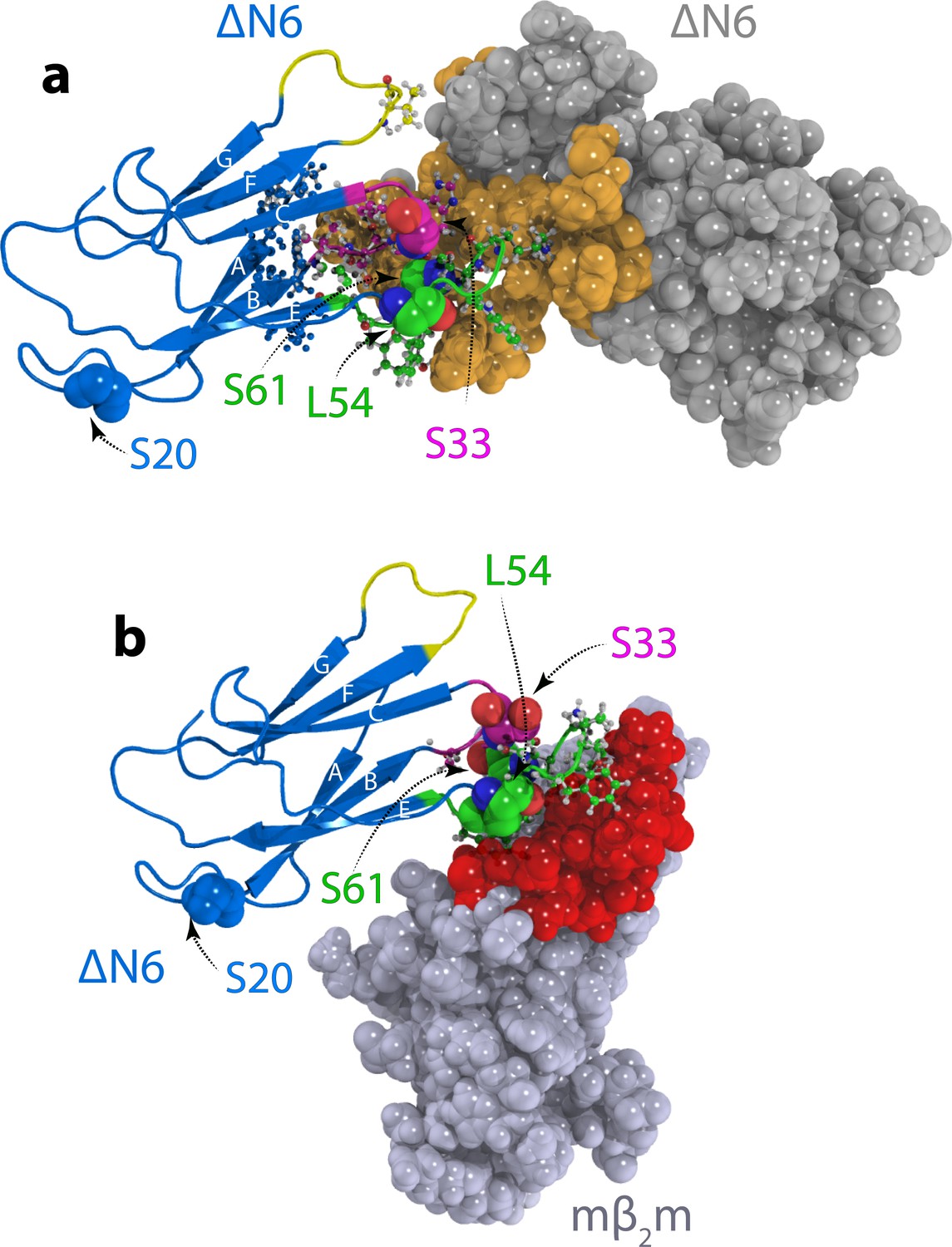
Structural models of ΔN6 dimers.
Structural models of (a) the lowest energy ΔN6 homodimer (dimer A) and (b) the ΔN6-mβ2m heterodimer that inhibits ΔN6 fibril assembly (Karamanos et al., 2014). Interface residues (identified as those residues that have any pair of atoms closer than 5 Å) are shown in a ball and stick representation on one subunit and are colored in space fill in gold in (a) or red in (b) on the surface of the second subunit. ΔN6 is shown in the same pose (blue) in (a) and (b). The BC, DE and FG loops are shown in magenta, green and yellow, respectively, and the position of attachment of MTSL for the PRE experiments (residues 20, 33, 54 and 61) is highlighted in spheres. PDB files are publicly available from the University of Leeds depository (https://doi.org/10.5518/329). See also Video 1.
Figure 4—figure supplement 1

Alternative ΔN6 dimer structures.
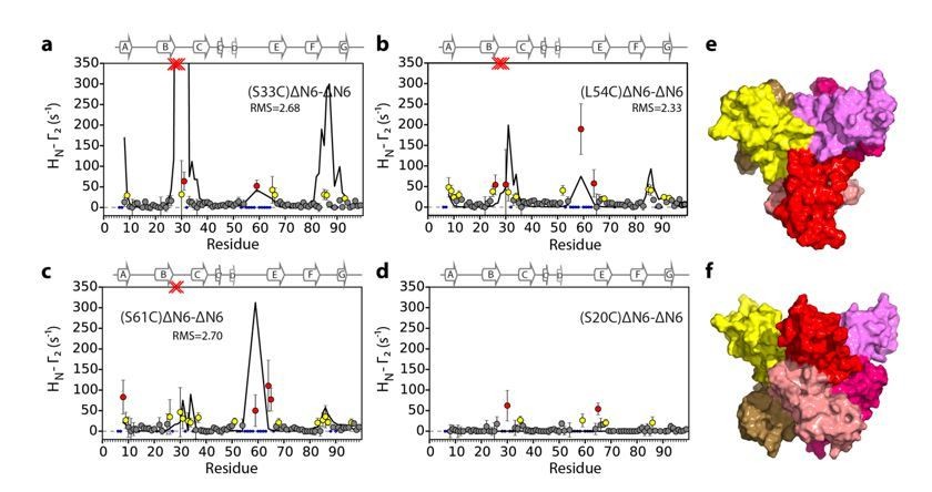
Intermolecular PRE data for the self-association of 15N-ΔN6 (60 μM) mixed with 60 μM of (a) 14N-(S33C)ΔN6-MTSL, (b) 14N-(L54C)ΔN6-MTSL, (c) 14N-(S61C)ΔN6-MTSL, or (d) 14N-(S20C)ΔN6-MTSL) with the PRE effect color-coded according to its amplitude (blue dot- residues not assigned, gray-insignificant (<20 s−1), yellow->20 s−1, red->50 s−1, pH 6.2, 25°C). Red crosses indicate high HN-Γ2 rates for which an accurate value could not be determined. Solid black lines represent back-calculated PREs from the high energy dimer structure shown in (e) and (f). The small PREs arising from14N-(S20C)ΔN6-MTSL result from non-specific interactions with MTSL itself. (e and f) The structural model of dimer B shown in different orientations. In each diagram, one subunit is shown in cartoon representation (BC loop (magenta), DE loop (green) and FG loop (yellow)) and the second is shown as a surface. Interface residues are highlighted as balls and sticks on the first subunit and shown in gold space-fill on the second subunit. The MTSL attachment sites are highlighted as spheres and the positions of attachment (20, 33, 54 or 61) are labeled. The interface in dimer B involves a more extensive inter-subunit interface in the apical loops than observed in dimer A (Figure 4a). The resulting interface for dimer B does not describe the PRE data (solid black line) as well as the lower energy model of dimer A shown in Figure 4a (Materials and methods and Table 1).
Figure 5 with 6 supplements

Structural model of ΔN6 hexamers.
(a–c) Sphere representations of the hexamer model formed from dimer A rotated by 90° in each view. Subunits belonging to the same dimer are colored in different tones of the same color. (d) The monomer-monomer (intra-dimer) interface is highlighted in green on the surface of the dimer formed from subunits 1a and 1b (within dimer A), with the other dimers shown as cartoons. (e) The inter-dimer interface is colored red on the surface of the dimer formed from subunits 1a and 1b, with the dimers shown as cartoons. (f) As in (e), but showing the dimer formed from subunits 1a and 1b, superposed with the mβ2m subunit in the inhibitory ΔN6-mβ2m dimer (Karamanos et al., 2014) (green cartoon). The ΔN6-ΔN6 and ΔN6-mβ2m dimers were aligned on the ΔN6 subunit 1b. Schematics of the assemblies are shown at the bottom colored as in (d–f). Note that the BC, DE and FG loops are highlighted as thicker chains in blue, green and cyan, respectively, in d-f. PDB files are publicly available from the University of Leeds depository (https://doi.org/10.5518/329). See also Video 2.
Figure 5—figure supplement 1

Intermolecular PREs at high ΔN6 concentration.
Intermolecular PRE data for the self-association of (a) 240 μM 15N-ΔN6 mixed with 80 μM 14N-(L54C)ΔN6-MTSL, (b) 200 μM 15N- ΔN6 mixed with 200 μM 14N-(L54C)ΔN6-MTSL, or (c) 80 μM 15N- ΔN6 mixed with 240 μM 14N-(S33C)ΔN6-MTSL. PRE data are color-coded according to their amplitude (blue dots-not assigned, gray-insignificant (<20 s−1), yellow->20 s−1, red->50 s−1, pH 6.2, 25°C). Red crosses indicate high HN-Γ2 rates for which an accurate value could not be determined. (d) Raw PRE data for residue 85V when 60 μM 14N-(L54C)ΔN6-MTSL was mixed with 60 μM 15N-ΔN6 (left) or when 200 μM 14N-(L54C)ΔN6-MTSL was mixed with 200 μM 15N-ΔN6 (right). Solid lines represent single exponential fits for the paramagnetic (black) or the diamagnetic samples (red).
Figure 5—figure supplement 2
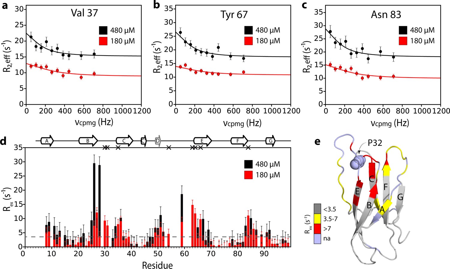
Additional interfaces do not form in the ΔN6 hexamer.
15N relaxation dispersion CPMG data for residues (a) 37, (b) 67, and (c) 83 at 180 μM ΔN6 (26% ΔN6 molecules are monomers, 48% are in dimers, 26% are in hexamers) (red) or 480 μM ΔN6 (13% ΔN6 molecules are monomers, 32% are in dimers, 55% are in hexamers) (black). Solid lines represent fits to the fast exchange model, yielding values of kexbind of 1790 ± 290 s−1 at 180 μM ΔN6 and kexbind of 1170 ± 196 s−1 at 480 μM ΔN6 (see Materials and methods). (d) Plots of Rex per residue defined as R2,eff50Hz - R2,eff680Hz. The dashed line represents one standard deviation of the mean calculated for all data points. Residues are numbered according to the WT sequence. Significant CPMG profiles are observed for residues in the N-terminus, A strand, BC, DE and FG loops, in excellent agreement with the intermolecular PRE data shown at 120 μM and 320 μM ΔN6 in Figure 3 and Figure 5—figure supplement 1. Residues which are severely broadened at 480 μM, thereby precluding accurate determination of their Rex values, are shown as black crosses. Crucially, when the protein concentration was increased the residues which show significant CPMG profiles are unchanged suggesting that the dimers and hexamers share a similar interface. (e) The structure of ΔN6 (2XKU; Eichner et al., 2011) colored according to the Rex amplitude as indicated in the scale bar. Trans Pro32 is shown in space-fill (pale blue).
Figure 5—figure supplement 3
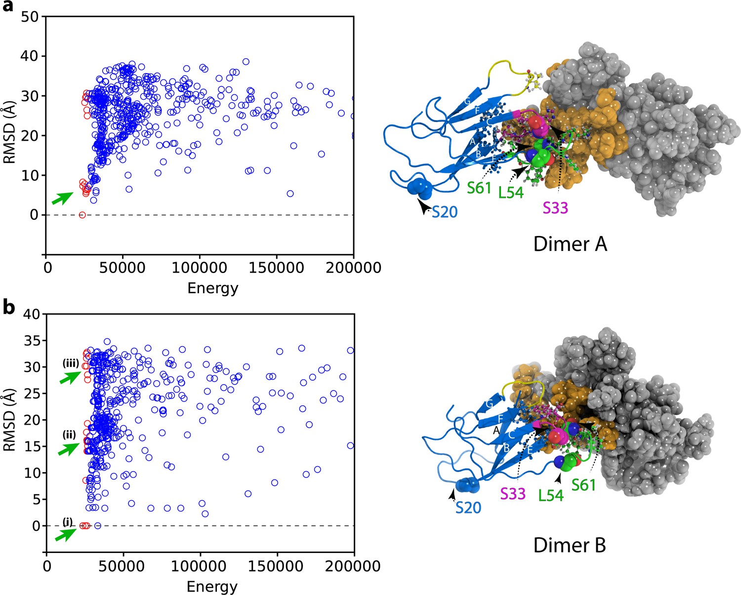
Initial docking of dimer structures to create hexamer models.
Plots of RMSD (to the lowest energy structure) versus total energy for hexamers generated by docking of (a) the lowest energy dimer structure (dimer A) or (b) the higher energy dimer (dimer B). The 50 lowest energy hexamer structures are marked as red circles. The hexamers that were selected for the next round of structure calculation for each dimer starting model are marked with green arrows. The structural model of dimer A and dimer B are shown alongside colored as in Figure 4—figure supplement 1.
Figure 5—figure supplement 4
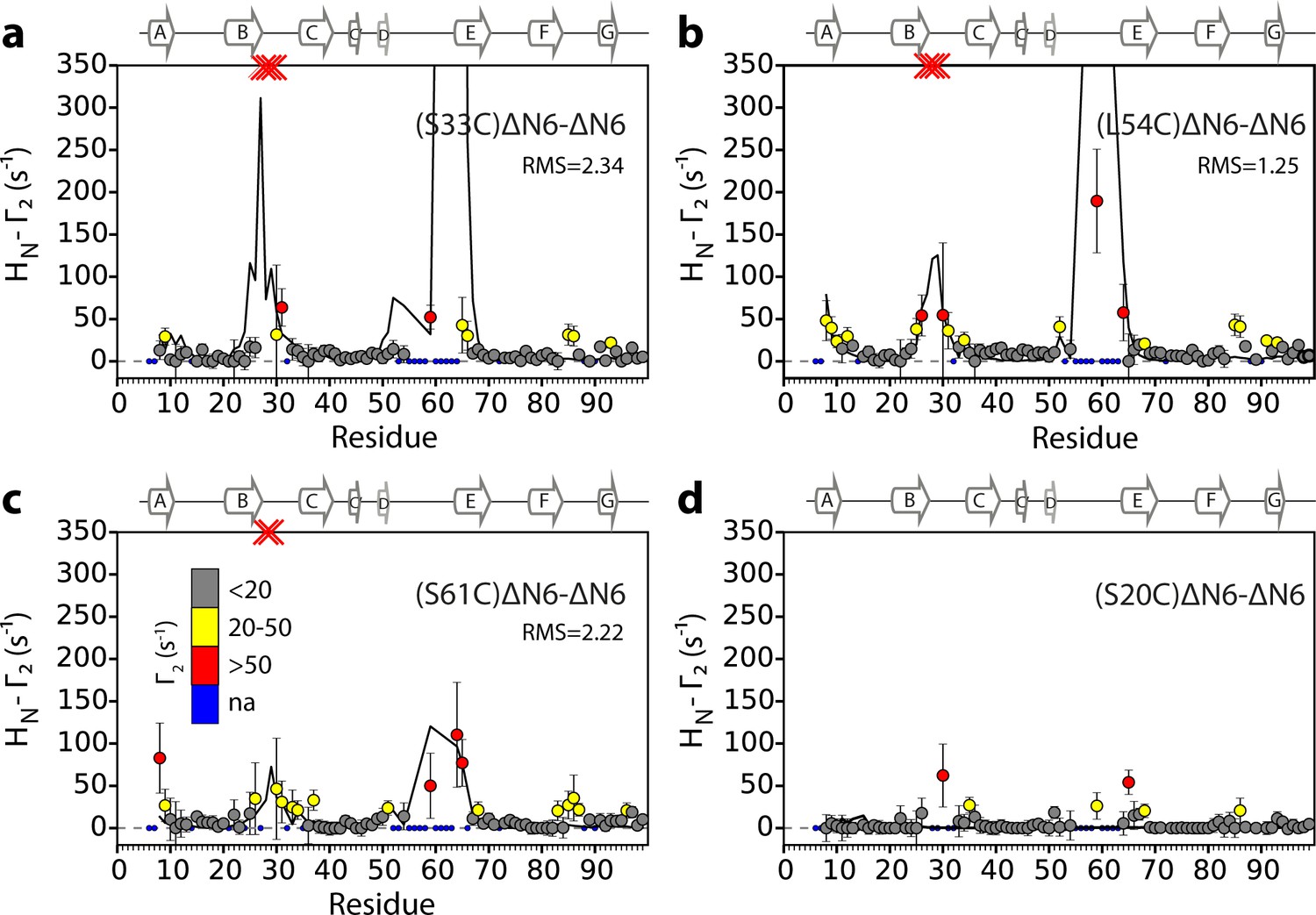
Intermolecular PREs back-calculated from the hexamer structural model generated from dimer A.
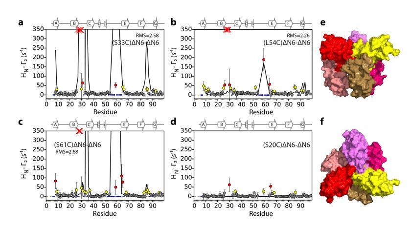
Intermolecular PRE data for the self-association of ΔN6. 15N- ΔN6 (60 μM) was mixed with 60 μM of (a) 14N-(S33C)ΔN6-MTSL, (b) 14N-(L54C)ΔN6-MTSL, (c) 14N-(S61C)ΔN6-MTSL, or (d) 14N-(S20C)ΔN6-MTSL. The data are color-coded according to their amplitude (blue dots-not assigned, gray-insignificant (<20 s−1), yellow->20 s−1, red->50 s−1, pH 6.2, 25°C). Red crosses indicate high HN-Γ2 rates for which an accurate value could not be determined. Solid black lines represent back-calculated PREs from the lowest energy hexamer structure (arising from dimer A) shown in Figure 5. The RMS distances (Å) between the intermolecular distances that were used as restraints and those back-calculated from the hexamer structural model are shown (inset) for each dataset (see Materials and methods).
Figure 5—figure supplement 5
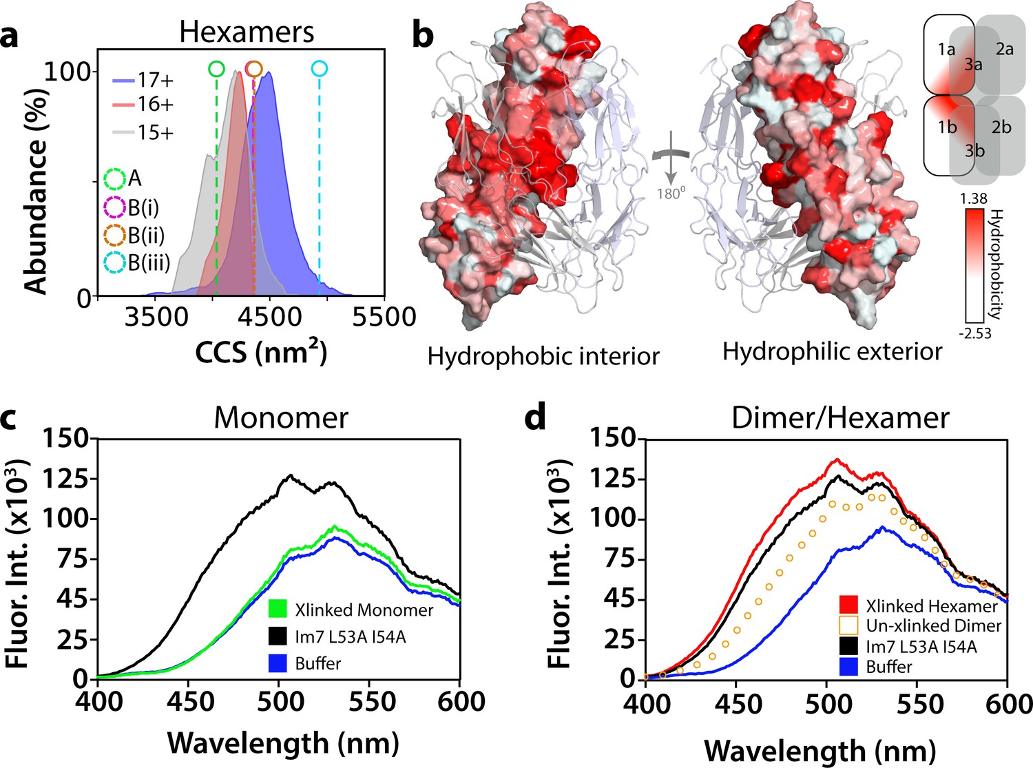
Conformational and biochemical properties of ΔN6 hexamers.
(a) ESI-IMS-MS analysis. Collision cross section (CCS) distributions for each observed charge state of hexameric ΔN6. The charge state for each CCS distribution is indicated. Note that the CCS of the lowest (most native; Vahidi et al., 2013) charge state (15+) is consistent with the hexamer model generated from dimer A (labeled A (green)), but not the models generated from dimer B (labeled (B(i)), (B(ii)) and (B(iii)) for the three conformers labeled in Figure 5—figure supplement 3b). (b) Hydrophobicity of the hexamer interface. The surface of dimer one in the hexamer is colored according to the Eisenberg hydrophobicity scale (Arg = −2.53, Ile = 1.38) (Eisenberg et al., 1984) with the other dimers shown as cartoons. A key is show alongside. The view on the left-hand side shows the surface that is packed against dimers 2 and 3 in the hexamer (interior), with the view on the right-hand side showing the exterior surface of the assembly. (c, d) Fluorescence emission spectra of ANS (200 μM) incubated with (c) ΔN6 monomers (green), (d) dimers (open symbols) or hexamers (red) (eluting at 17 mL, 15 mL and 11 mL, respectively obtained with/without cross-linking, as indicated, using SEC; Figure 5—figure supplement 6). The fluorescence emission spectrum of ANS in buffer alone is shown in blue. ANS bound to the partially folded Im7 variant L53A I54A (Spence et al., 2004) (1 μM) is shown for comparison (black). This was used as a model for a compact native-like folding intermediate (Spence et al., 2004) (see text).
Figure 5—figure supplement 6
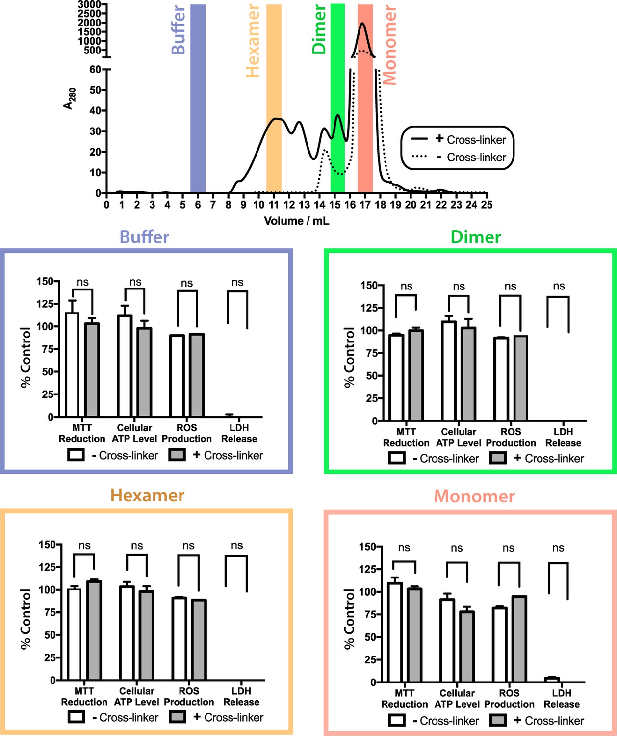
ΔN6 oligomers are not cytotoxic to SH-SY5Y cells.
Toxicity of cross-linked (solid line/gray bars) or uncross-linked (dotted line/white bars) ΔN6 species following purification by analytical SEC. Cell toxicity was assessed using MTT reduction, cellular ATP level, generation of reactive oxygen species (ROS), and LDH release assays. For assays of MTT reduction, ATP levels and ROS production, the data are normalized to PBS (100%) and NaN3-treated controls (0%). LDH release is normalized to detergent lysed cells (100%) and PBS buffer treated controls (0%). The error bars represent mean S.E, * p 0.05. No evidence for cytotoxicity was observed for any protein species under the conditions employed.
Figure 6 with 1 supplement
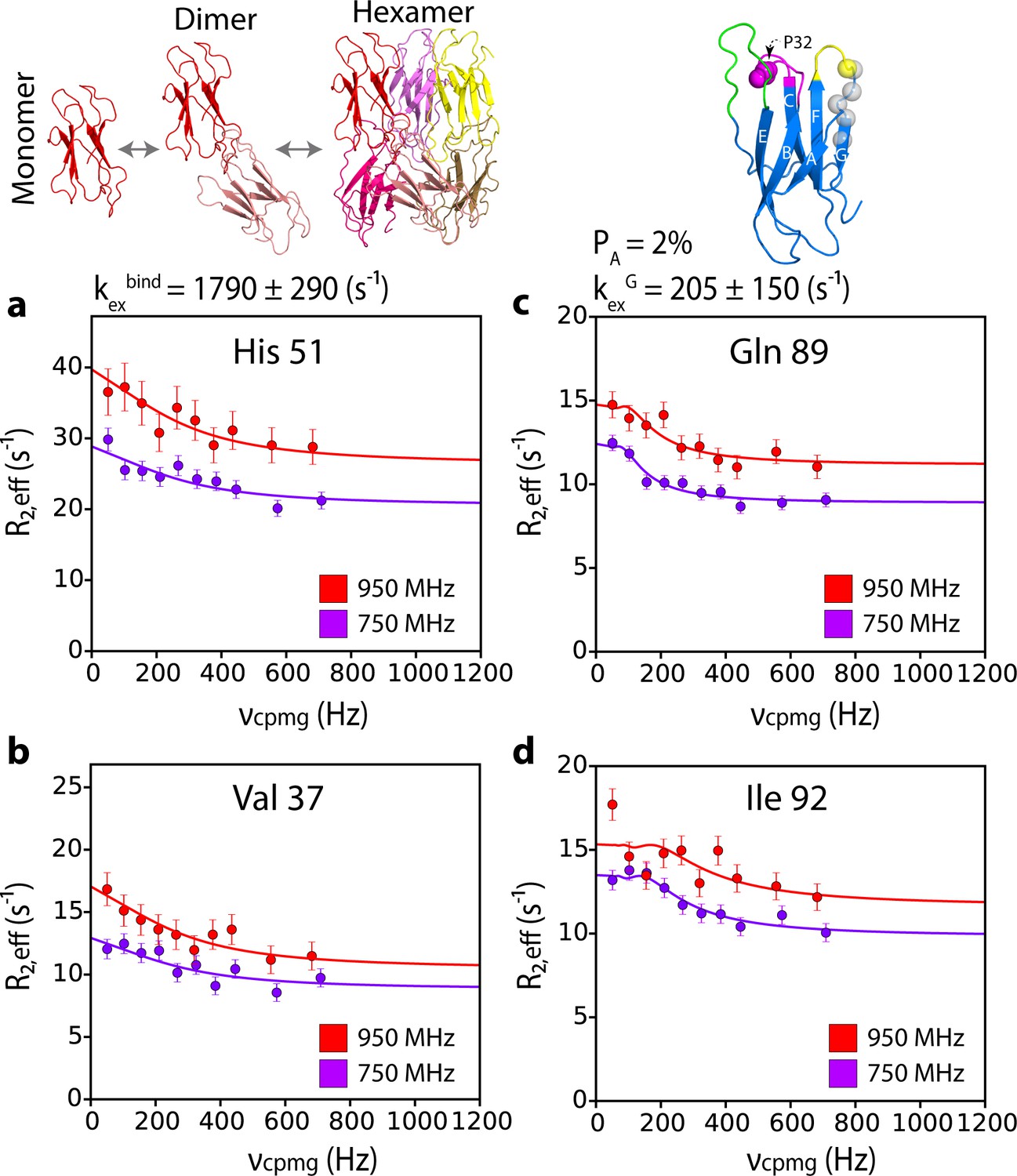
G-strand unfurling may occur upon hexamer formation.
15N CPMG relaxation dispersion data at 750 MHz (magenta) and 950 MHz (red) (180 μM ΔN6, pH 6.2 (26% ΔN6 molecules are monomers, 48% are in dimers, 26% are in hexamers) for residues (a) 51, (b) 37, (c) 89, and (d) 92. Residues 37 and 51 report on intermolecular interactions that describe dimer and/or hexamer formation (schematic, top left), while residues 89 and 92 do not lie in an interface and report instead in the dynamics of the G strand in the different assemblies formed. The position of all five residues used in the cluster analysis of G strand dynamics is shown in spheres on the structure of ΔN6 (blue cartoon, top right). Pro32 is shown as a magenta sphere. Solid lines represent global fits to the Bloch-McConnell equations (Materials and methods) for each cluster of residues. The extracted parameters of the global fit for the two processes (kexbind and kexG) are indicated above the plots.
Figure 6—figure supplement 1

Hexamer formation increases the dynamics of the G strand.
(a) Location of the G strand in relation to the dimer and hexamer interfaces. Dimer one in the hexamer is shown in a cartoon representation while dimers 2 and 3 are shown as semi-transparent surfaces. The positions of the amide protons for residues 87, 89, 91, 92 are shown as gray spheres and the residues that take part in both the dimer and hexamer interfaces are shown as red spheres on the structure of dimer 1. A schematic of the assembly is shown alongside. 15N relaxation dispersion CPMG data for residues (b) 87, (c) 89, (d) 91 and (e) 92 at 950 MHz (red) and 750 MHz (magenta) of 180 μM ΔN6, pH 6.2. Solid lines represent the global fits to all residues in the cluster to the slow exchange model which yields a kexG of 205 ± 150 s−1. CPMG data for the same residues (f) 87, (g) 89, (h) 91 and (i) 92 at 750 MHz (blue) and 600 MHz (gray) using 480 μM ΔN6. Solid lines represent global fits to the fast exchange model which yields a kexG of 1170 ± 196 s−1.
Figure 7 with 1 supplement
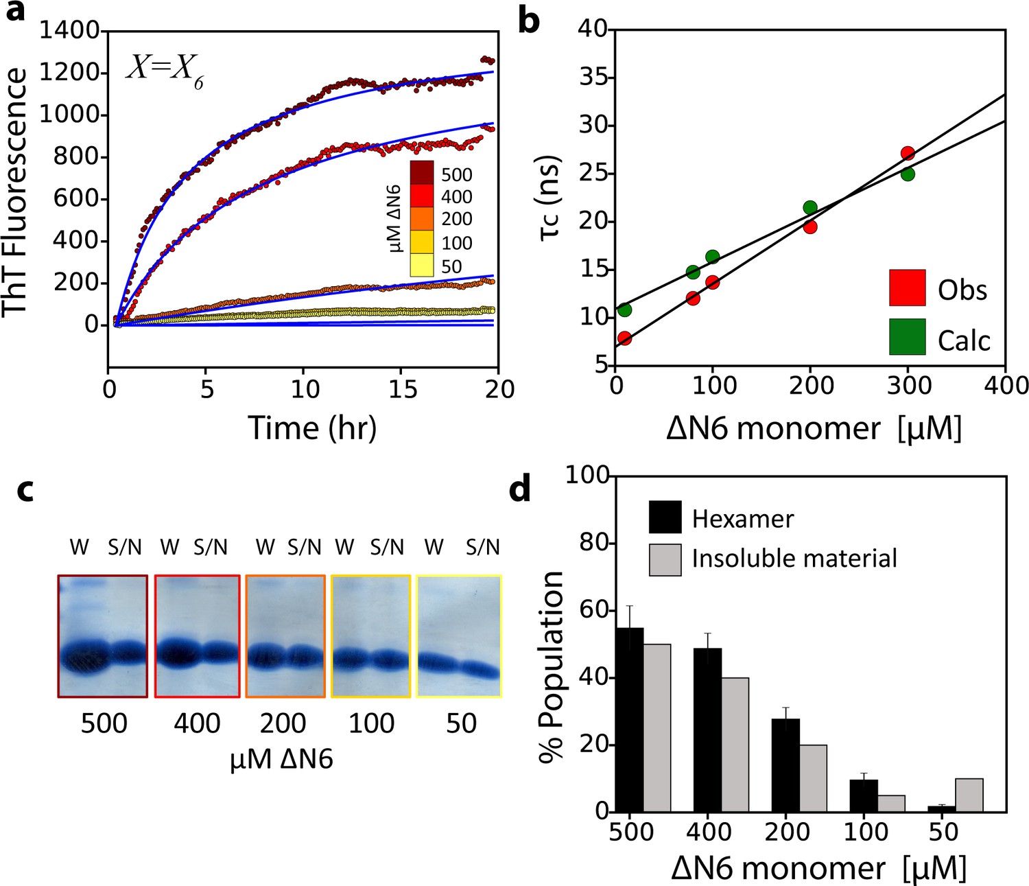
The monomer-dimer-hexamer model describes the thermodynamics and kinetics of fibril elongation.
(a) Global fits (blue solid lines) to the fibril elongation kinetics monitored by ThT fluorescence assuming a hexamer addition model at different concentrations of soluble ΔN6 (dots) (Materials and methods and Table 4). The concentrations of ΔN6 are colored according to the key. The average of five replicates is shown. (b) Protein correlation times (τc) measured using NMR (red) and back-calculated values (green) using the populations of monomers, dimers and hexamers predicted from the monomer-dimer-hexamer model and the correlation times of the dimers and hexamer structural models shown in Figures 4 and 5. (c) The fibril yield (after 100 hr) of each elongation reaction. SDS-PAGE analysis of the whole reaction (shown in (a)) before centrifugation (W) or of the supernatant (S/N) after centrifugation at the different concentrations of ΔN6, as indicated. (d) Bar-charts showing the % of insoluble material (gray) measured using densitometry of the gel shown in (c). The % hexamer population in the absence of seeds (black) predicted by the monomer-dimer-hexamer model at each ΔN6 concentration correlates with the % insoluble material (gray). Note that the fibril yield is low since fibrils cannot form when the monomer concentration falls significantly below the Kd for dimer formation (50 μM).
Figure 7—figure supplement 1
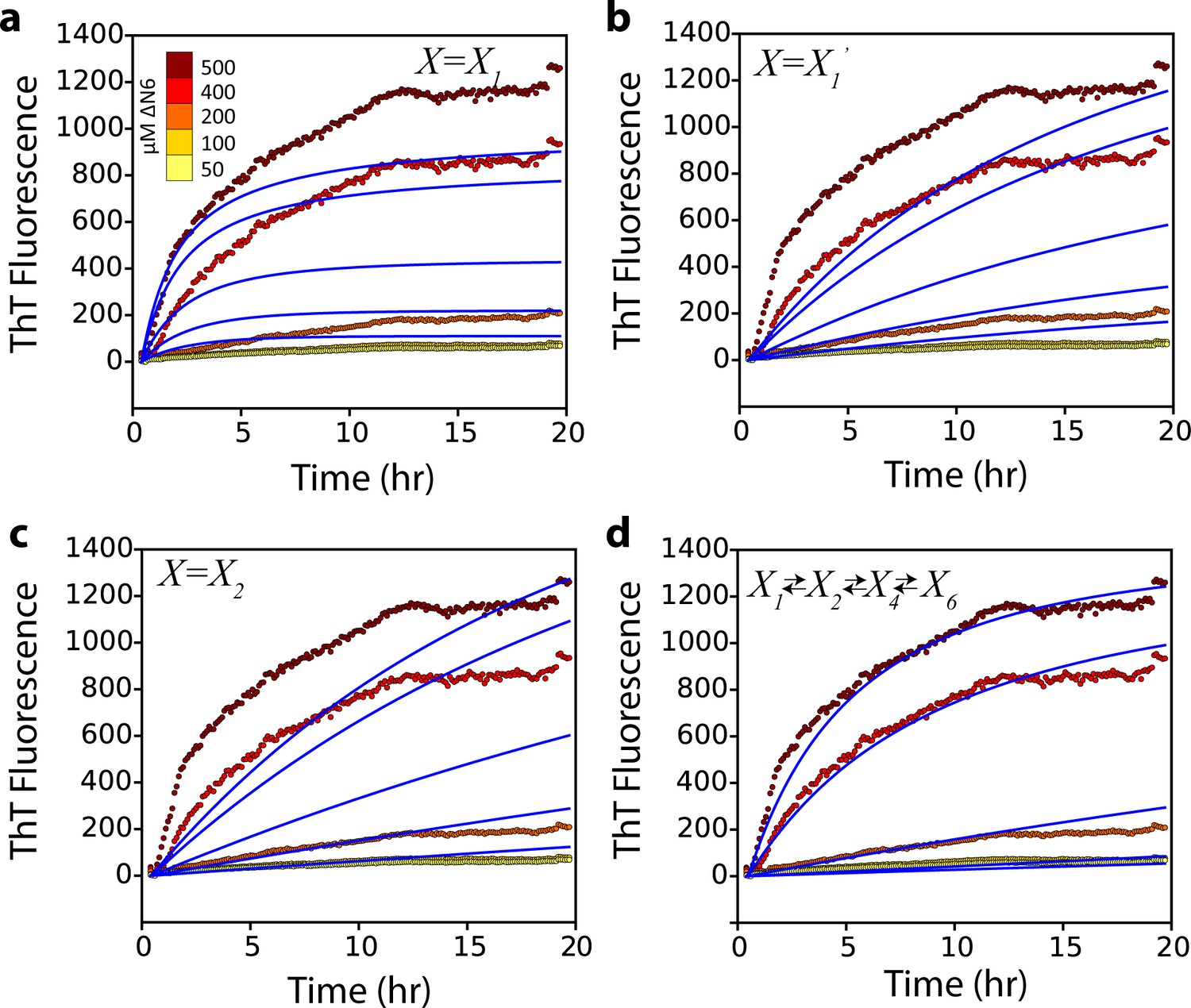
Alternative kinetic models do not describe the kinetics of seeded fibril growth.
Global fits (blue solid lines) which assume that (a) a monomer, (b) a monomer excited state, or (c) a dimer, add to the fibril ends do not describe the observed fibril growth kinetics monitored using ThT fluorescence at different concentrations of soluble ΔN6 (dotted lines and key). A more complex monomer-dimer-tetramer-hexamer model (d) does not improve the quality of the fit compared with that shown in Figure 7a.
Figure 8 with 2 supplements
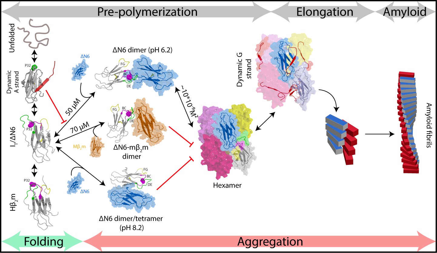
Fibril formation in atomic detail.
Schematic representation of the mechanism of amyloid formation for ΔN6. During folding of hβ2m, a highly dynamic intermediate with a flexible A strand is populated prior to formation of the native-like intermediate termed ΙT, which has a native-like fold but contains a non-native trans X-Pro32 bond. The latter species is mimicked by ΔN6 and formed in vivo by proteolytic degradation of the WT protein (Bellotti et al., 1998). Only IT/ΔN6 is primed for aggregation, while the intermediate with the flexible A strand is not able to assembly directly into amyloid (Karamanos et al., 2016). As reported here, ΔN6 forms elongated head-to-head dimers (upper image, center) which assemble into hexamers. Alternative dimers involving interactions between the ABED β-sheets in adjacent molecules formed at pH 8.2 (lower image, center) do not associate further into fibrils. Murine β2m (mβ2m) also interacts with ΔN6 at pH 6.2 to form head-to-head heterodimers. The subunit orientation is different in this heterodimer (Karamanos et al., 2014), occluding the hexamer interface and inhibiting assembly (central image). ΔN6 hexamers can elongate fibrillar seeds and show enhanced dynamics in the G strand which could represent the first step towards the major structural reorganization required to form the parallel in-register amyloid fold. How this final step occurs, however, remains to be solved.
Figure 8—figure supplement 1
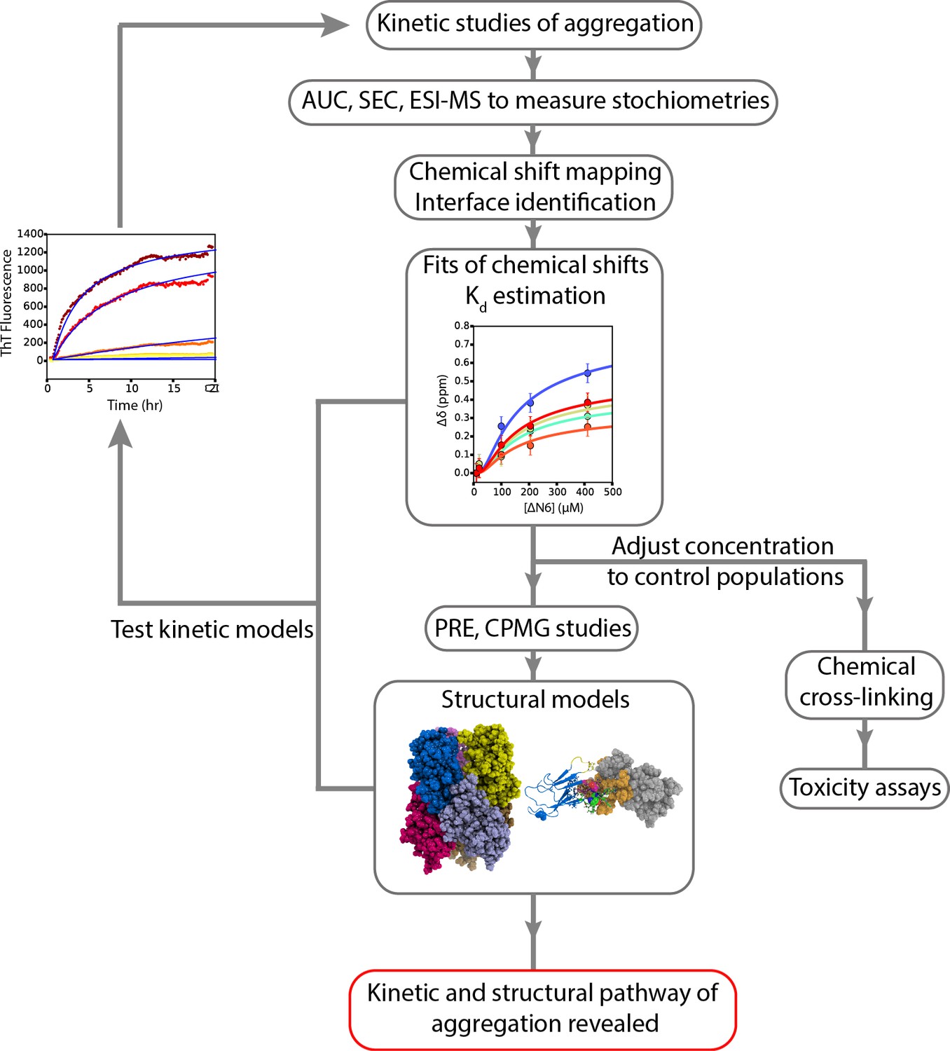
A workflow to enable weakly self-assembling systems to be analyzed in structural, kinetic and thermodynamic detail.
A schematic overview of the strategy employed to study the aggregation of ΔN6 which can be extended to other systems. Careful examination of kinetic rates of aggregation leads to the identification of possible aggregation pathways. Structural methods (AUC, SEC, cross-linking, ESI-IMS-MS) can then be used to identify the molecular weight and collision crosssection of the species involved. NMR chemical shift analysis and measurements of RDCs can be used to determine estimates of Kd which in turn can be used to determine conditions under which different species are populated. More detailed NMR studies lead to structural models of these species, while stabilization of the intermediates by chemical cross-linking aids the assessment of their cytotoxicity. The structural and kinetic information collected leads to the generation of kinetic models whose ability to describe the progress of aggregation monitored by ThT fluorescence is tested using numerical methods. Agreement is suggestive of the validity of the kinetic mechanism of assembly and the identity and structural properties of oligomeric intermediates formed.
Figure 8—figure supplement 2
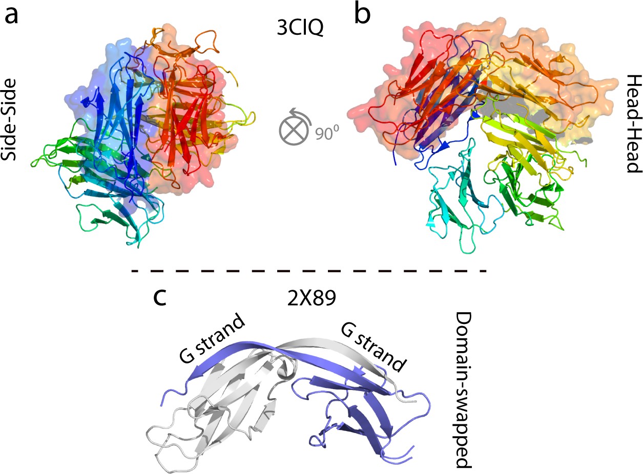
Examples of some previously characterized oligomers of WT hβ2m and ΔN6.
(a, b) Cu2+-stabilized H13F hβ2m hexamer (Calabrese et al., 2008; Eakin et al., 2004; Calabrese and Miranker, 2007; Antwi et al., 2008). (c) Domain swapped ΔN6 dimer (Domanska et al., 2011).
Author response image 1
Evaluation of hexamer i, assembled for dimer B.
Back-calculated PRE rates (black lines) are shown in panels A-D. Top (E) and side (F) view of the structural model.
Author response image 2
Evaluation of hexamer ii, assembled for dimer B.
Back-calculated PRE rates (black lines) are shown in panels A-D. Top (E) and side (F) view of the structural model.
Author response image 3

Evaluation of hexamer iii, assembled for dimer B.
Back-calculated PRE rates (black lines) are shown in panels A-D. Top (E) and side (F) view of the structural model.
Author response image 4
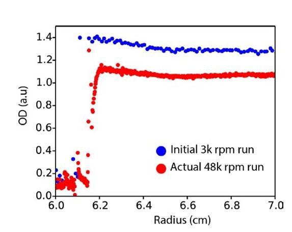
Raw AUC data.
Plot of absorbance at 280 nm across the AUC cell radius for the initial run (3000 rpm, blue) versus the first scan of the actual run at 48000 rpm (red).
Videos
Video 1
Comparison of productive and inhibitory dimers.
The ΔN6 subunit in each dimer (this study) is shown as a dark blue cartoon, while the second ΔN6 monomer in the productive dimer and the mβ2m subunit in the inhibitory dimer (Karamanos et al., 2014) are shown as light blue and red, respectively. The BC, DE, FG loops are colored in magenta, green and yellow, respectively, while the intra-dimer interface residues are shown as sticks on both subunits.
Video 2
ΔN6 assembles into dimers and hexamers.
The two ΔN6 subunits in the dimer (dimer A) are shown as blue cartoon and gray cartoon/transparent space-filling representations, respectively. The BC, DE and FG loops are colored magenta, green and yellow, respectively. The intra-dimer interface residues are shown as sticks on one subunit and as orange transparent spheres on the second subunit. The hexamer assembly is then shown as a space-filling model, with dimer one shown in dark blue/light blue, dimer two in dark yellow/light yellow and dimer three in magenta/pink. In the last part of the video only dimer one is shown as spheres while dimers 2 and 3 are shown as transparent cartoons. The intra-dimer interface is shown in green and the inter-dimer interface is shown in red.
Tables
Table 1
Agreement between experimental and back-calculated intermolecular PREs for the two dimer structures (dimer A and dimer B (see Figure 5—figure supplement 3).
RMS values are shown comparing the measured versus the predicted values from the structure PREs measured from S33, L54 and S61. Data from position S20 were not used as they arise from non-specific interactions with MTSL.
| PRE term | RMS dimer A | RMS dimer B |
|---|---|---|
| S33C(ΔN6)-ΔN6 (s−1) | 18.65 | 15.10 |
| L54C(ΔN6)-ΔN6 (s−1) | 29.02 | 27.44 |
| S61C(ΔN6)-ΔN6 (s−1) | 19.44 | 23.27 |
| *High PREs (Å) | 2.78 | 3.79 |
-
*High PREs refer to PREs in the BC loop (measured from S33, L54 and S61) that (due to their large value) could not be measured accurately and therefore are incorporated as loose distance restraints.
Table 2
Agreement between experimental and back-calculated intermolecular distances for different hexamer structures.
RMS values are shown comparing the measured versus the predicted distances from each structural model for distances measured from S33, L54 and S61. Data from position S20 were not used as they arise from non-specific interactions with MTSL. See also Figure 5—figure supplement 3.
| PRE term | Hexamer 1 RMS (Å) | Hexamer 2(i) RMS (Å) | Hexamer 2(ii) RMS (Å) | Hexamer 2(iii) RMS (Å) |
|---|---|---|---|---|
| S33C(ΔN6)-ΔN6 | 2.34 | 2.68 | 2.58 | 2.53 |
| L54C(ΔN6)-ΔN6 | 1.25 | 2.33 | 2.26 | 1.87 |
| S61C(ΔN6)-ΔN6 | 2.22 | 2.7 | 2.68 | 3.11 |
Table 3
Analysis of dimer and hexamer interfaces.
The buried surface area is calculated as the sum for the two subunits for each complex. Interface residues were identified as those residues that lose at least 10% of accessible surface area upon oligomer formation.
| ΔN6 dimer A | ΔN6 hexamer | |
|---|---|---|
| Buried Surface Area (Å2) | 1233 | 4201 |
| % Charged residues in the interface | 28 | 18 |
| % Hydrophobic residues in the interface | 44 | 54 |
Table 4
Reaction schemes, rate equations and rate constants for the fibril elongation models tested.
X represents the species that add onto the fibril ends.
| Module | Variant | Reaction scheme | Rate equations | Rate constants |
|---|---|---|---|---|
| Pre-polymerization | No Pre-polymerization (Monomer addition) | | ||
| Monomer conformational exchange | | | | |
| Dimer addition | | | | |
| Hexamer addition | | | , | |
| Monomer-Dimer-Tetramer-Hexamer | | | | |
| Polymerization | |
Additional files
-
Transparent reporting form
- https://doi.org/10.7554/eLife.46574.031
Download links
A two-part list of links to download the article, or parts of the article, in various formats.
Downloads (link to download the article as PDF)
Open citations (links to open the citations from this article in various online reference manager services)
Cite this article (links to download the citations from this article in formats compatible with various reference manager tools)
Structural mapping of oligomeric intermediates in an amyloid assembly pathway
eLife 8:e46574.
https://doi.org/10.7554/eLife.46574


