Multi-phosphorylation reaction and clustering tune Pom1 gradient mid-cell levels according to cell size
- University of Lausanne, Switzerland
- École Polytechnique Fédérale de Lausanne (EPFL), Switzerland
Figures
Figure 1 with 3 supplements
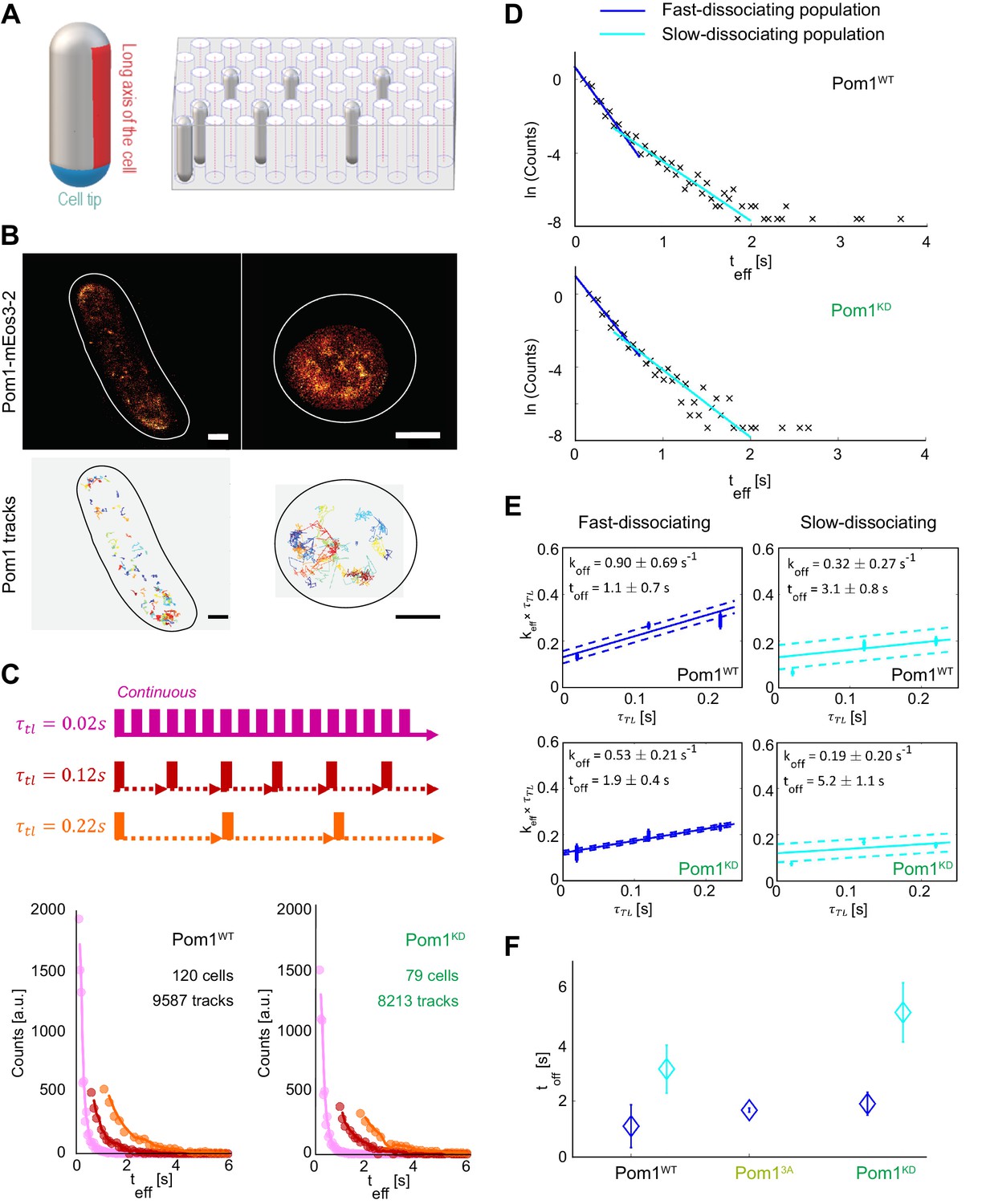
Pom1 dissociation dynamics.
(A) (left) Scheme of the cell regions imaged on flat pads (cell side, red) or vertical molds (cell pole, blue). (right) Scheme of the mold used for vertical immobilization in agar. (B) PALM reconstruction of Pom1 on the cell side (top left) or the cell pole (top right). White lines correspond to cell boundaries. Corresponding sptPALM tracks on the side (bottom left) and on the pole (bottom right). Scale bar 1 µm. (C) Scheme for time-lapse imaging experiments. Every frame is recorded with a 20ms exposure time (solid rectangles). A time delay (dashed arrows) is introduced between each pair of consecutive frames. The time-lapse period () is the sum of the integration time and the time delay. Effective residence time distributions for Pom1WT and Pom1KD, color correspond to different . (D) Residence time distributions for Pom1WT and Pom1KD, fit with a bi-exponential decay: fast (blue) and slow (cyan). (E) Effective rate constant as a function of time lag condition (symbols) for fast (blue) and slow (cyan) populations. Solid lines correspond to a weighted linear fit according to Equation 2. Error bars correspond to the weights associated to each data point (S.D. from the fit of the exponential distribution of the residence time obtained according to Equation 1 in Methods). (F) Comparison of the Pom1 residence time obtained for each subpopulation (fast in blue and slow in cyan) for Pom1WT, Pom13A and Pom1KD strains. Error bar corresponds to the standard deviation of the parameter extracted from the weighted linear fit of panel 1E.
Figure 1—figure supplement 1
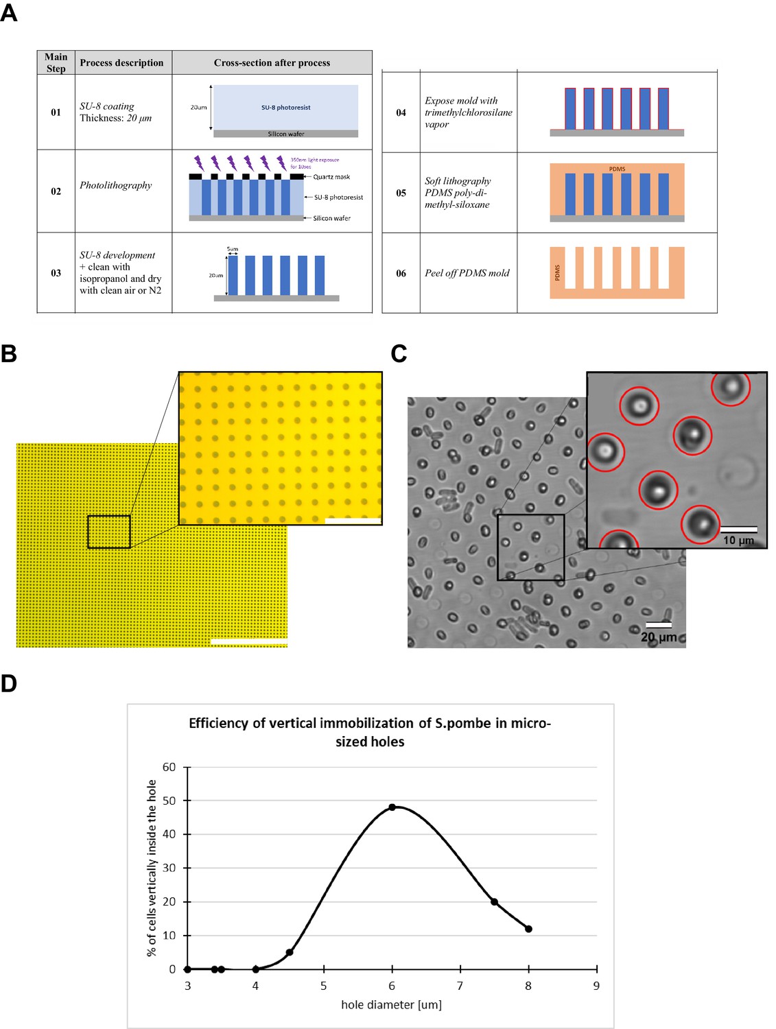
Fabrication of micro-holes for S. pombe cell vertical immobilization.
(A) Main steps of the process flow for the fabrication of the mold for the generation of the agarose support with micro-holes for vertical cell trapping. (B) Wide-field image of the quartz mask for photolithography. Scale bar 400 µm and 40 µm (magnified view). (C) Visual inspection of the micro-hole provided the identification and count of cells correctly placed. Scale bar 20 µm and 10 µm (magnified view). (D) To identify the optimal micro-hole diameter we fabricated different cell supports with the diameter size swept from 3 µm up to 8 µm. We found that the diameter size at which the maximum number of cells were correctly verticalized was around 6 µm.
Figure 1—figure supplement 2
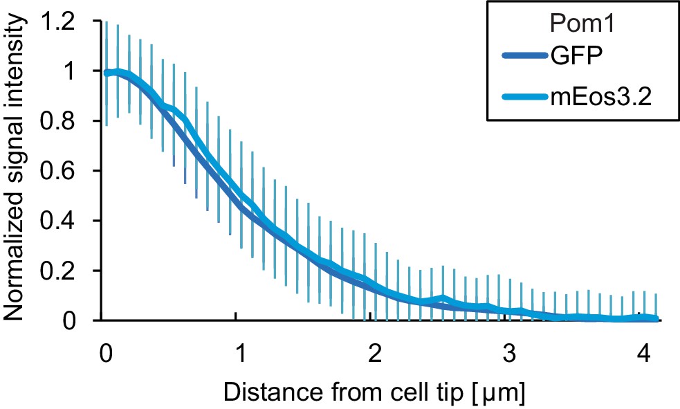
Comparison of Pom1-GFP and Pom1-mEos3.2.
Fluorescence intensity plots of normalized cortical gradient profiles, collected from time-average medial plane confocal images as in Figure 4. Error bars are standard deviation of the biological variation.
Figure 1—figure supplement 3
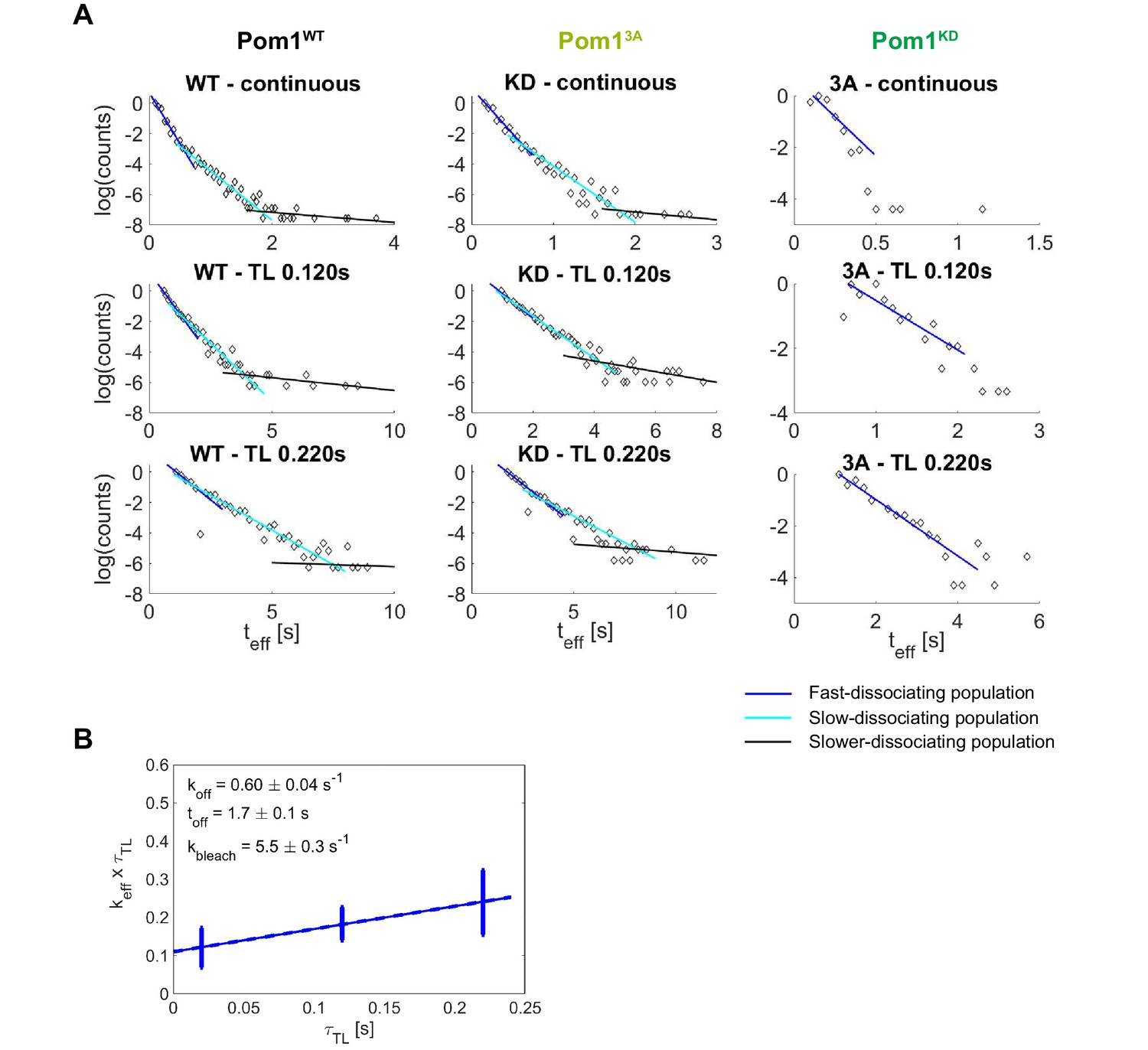
Pom1 dissociation analysis.
(A) Three-population identification and analysis through the fit of the exponential track length distribution. The last population (black) was excluded from the quantitative analysis due to the small sample size but was used to limit the second population (cyan). (B) Weighted linear fit of versus for Pom13A from which the dissociation rate constant and dissociation time constant are extracted according to Equation 2. Error bars correspond to the weights associated to each data point (S.D. from the fit of the exponential distribution of the track length).
Figure 2 with 2 supplements
Pom1 diffusion dynamics.
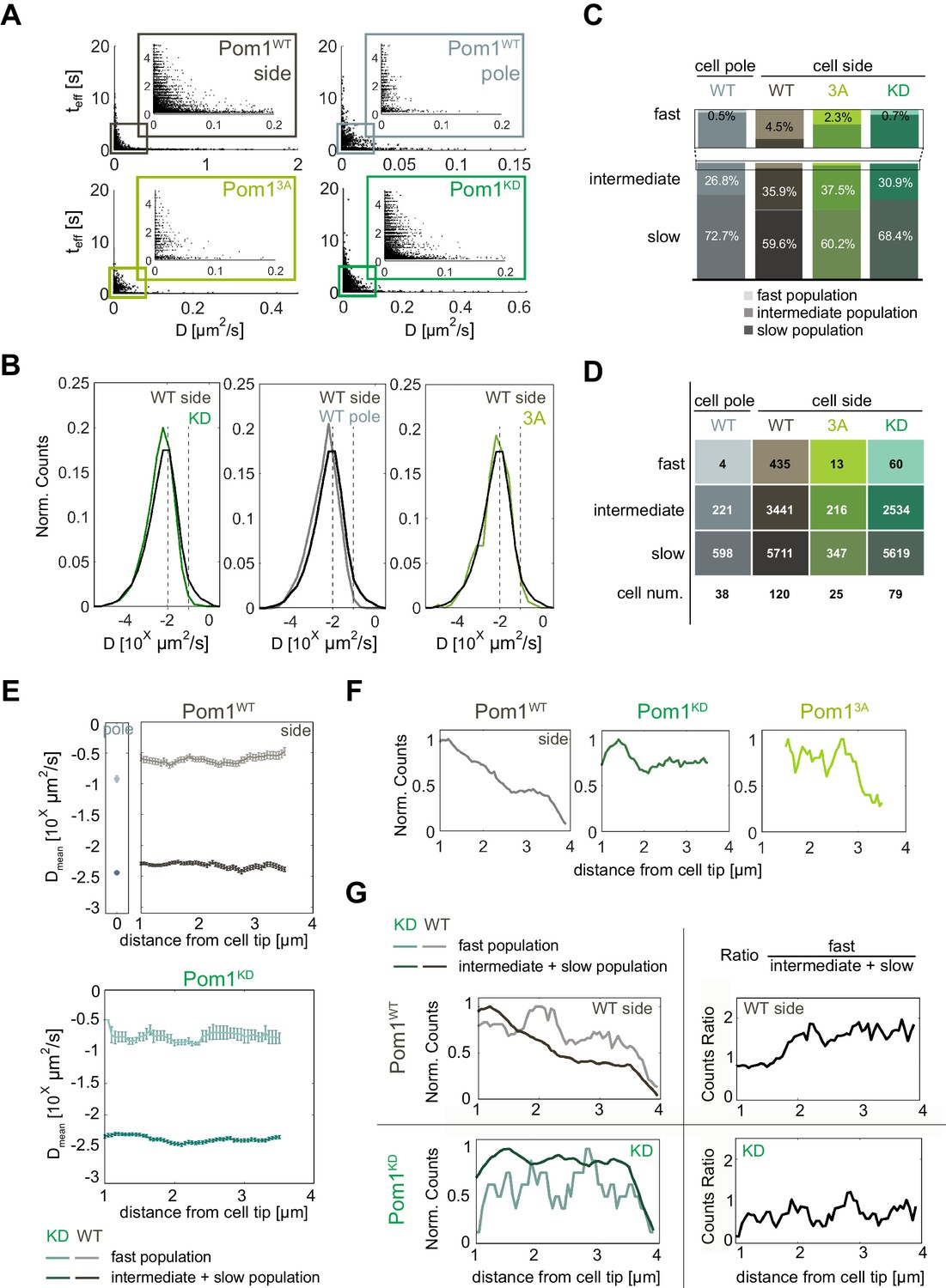
(A) Track length as a function of diffusion coefficients of the tracks for Pom1WT (WT) at cell sides (dark grey) and cell poles (light grey), Pom13A (3A; light green), Pom1KD (KD; green-cyan). Pom13A and Pom1KD were imaged at cell sides. (B) Distribution of diffusion coefficients of all Pom1 molecules tracked in Pom1WT, Pom13A and Pom1KD at cell sides, and Pom1WT at cell poles. Thresholds used in panels C-G are shown by the dashed lines.(C) Proportion of fast (D ≥ 10−1 µm2/s; light), intermediate (10−2 ≤ D < 10−1 µm2/s; medium color) and slow (D < 10−2 µm2/s; dark) populations for Pom1WT, Pom13A and Pom1KD at cell sides, and Pom1WT at cell poles. (D) Number of tracks and cells for each condition. (E) Average diffusion coefficient as a function of the distance from the pole for fast (D ≥ 0.1 µm2/s; light color) and combined intermediate and slow (dark) populations for Pom1WT (D < 0.1 µm2/s; top panels) and Pom1KD (bottom) strains. Error bar corresponds to standard error of the mean. (F) Evolution of count of all tracks along the cell length normalized by the maximum occurrence for Pom1WT, Pom1KD and Pom13A. (G) Evolution of the number of tracks for fast (D ≥ 0.1 µm2/s; light color) and combined intermediate and slow (D < 0.1 µm2/s; dark) populations along the cell length for Pom1WT and Pom1KD strains (left panels) and their ratio (right panel) for Pom1KD and Pom1KD strains. The color coding dark grey = Pom1WT at cell sides, light grey = Pom1WT at cell poles, green-cyan = Pom1KD, and light green = Pom13A is used throughout the figure.
Figure 2—figure supplement 1
Pom1 diffusion coefficient analysis with different thresholds.
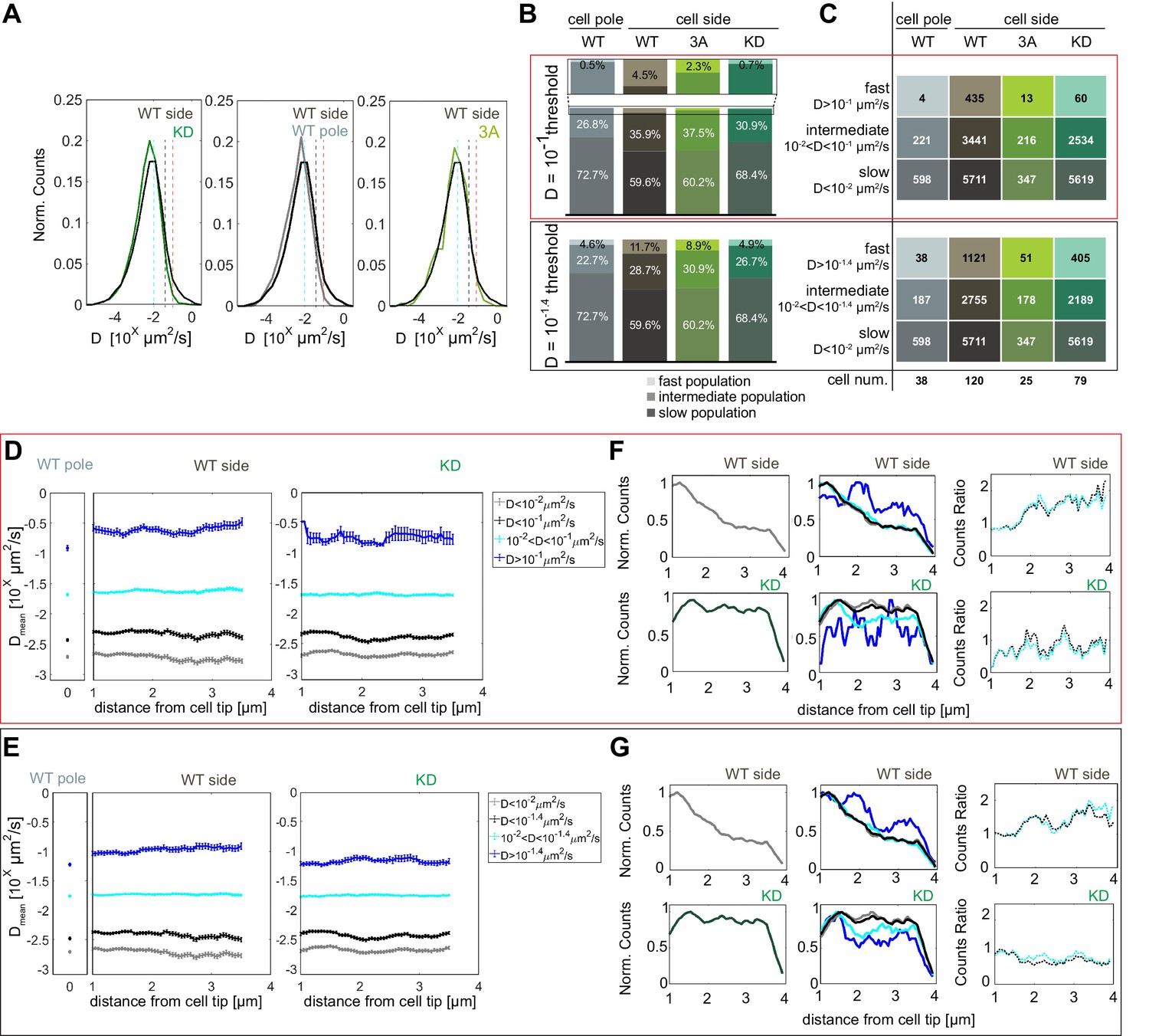
(A) Distribution of diffusion coefficients of all Pom1 molecules tracked in Pom1WT (dark grey), Pom13A (light green) and Pom1KD (green-cyan) at cell sides, and Pom1WT at cell poles (light grey), as in Figure 2B. The two thresholds set to delimit the fast from the intermediate populations are represented by the vertical red (D = 10−1 µm2/s) and grey (D = 10-1.4 µm2/s) lines. The cyan line (D = 10−2 µm2/s) delimits the intermediate from the slow populations. (B) Proportion of fast (light), intermediate and slow (dark) populations for Pom1WT, Pom13A and Pom1KD at cell sides, and Pom1WT at cell poles. (C) Number of tracks and cells for each condition. (D–E) Average diffusion coefficient as a function of the distance from the pole for fast (blue), intermediate (cyan), slow (grey) and intermediate plus slow (black) populations for Pom1WT at the pole (left panel), Pom1WT at the side (central panel) and Pom1KD (right panel) strains. Error bar corresponds to standard error of the mean. (F–G) Evolution of the total number of tracks for Pom1WT (dark gray, top-left panel) and Pom1KD (green-cyan, bottom-left panel) strains. Evolution of the number of tracks for fast (blue), intermediate (cyan), slow (grey) and slow plus intermediate (black) populations along the cell length for Pom1WT (top-central panel) and Pom1KD (bottom-central panel) strains. Ratios between the fast and intermediate population (cyan) and between fast and combined intermediate and slow population (black) for Pom1WT (top-right panel) and Pom1KD (bottom-right panel). For (B, C, D, F), the analysis in the red box uses D ≥ 10−1 µm2/s for the fast populations, 10−2 < D < 10−1 µm2/s for the intermediate populations and D < 10−2 µm2/s for the slow population. For (B, C, E, G) the analysis in the black box uses D ≥ 10-1.4 µm2/s for the fast populations, 10−2 < D < 10-1.4 µm2/s for the intermediate populations and D < 10−2 µm2/s for the slow population.
Figure 2—figure supplement 2
Pom13A diffusion coefficient analysis with different thresholds.
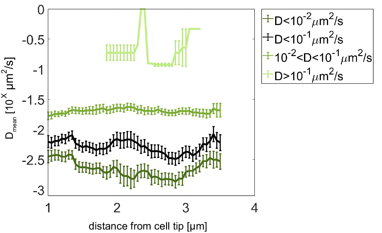
Average diffusion coefficient as a function of the distance from the pole for fast population (light green, D ≥ 10−1 µm2/s), intermediate (medium green, 10−2 < D < 10−1 µm2/s), slow (dark green, D < 10−2 µm2/s), and slow plus intermediate (black, D < 10−1 µm2/s) populations. Error bar corresponds to standard error of the mean.
Figure 3 with 1 supplement
Two distinct regions define Pom1 membrane binding.
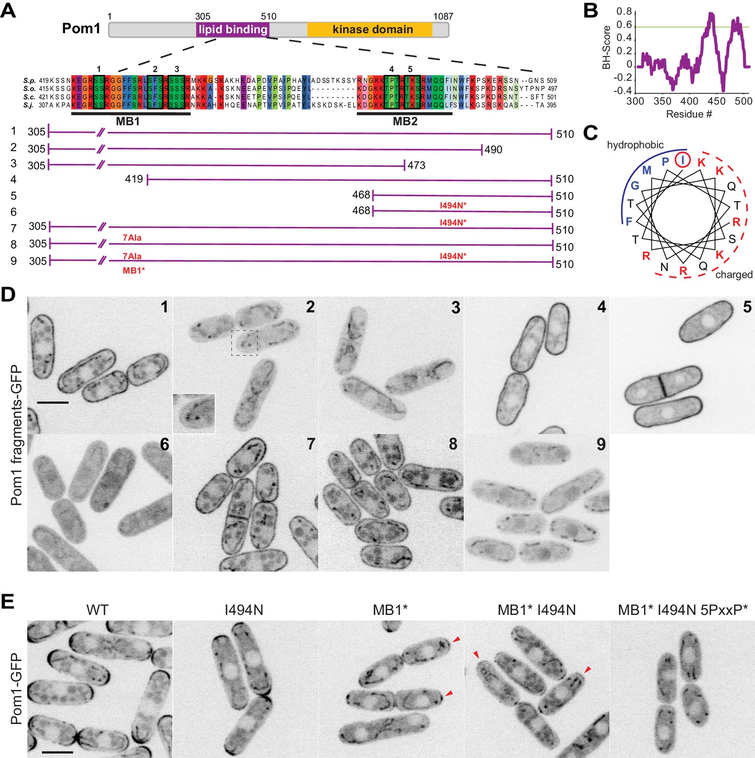
(A) Schematic representation of Pom1 with sequence homology alignment of the lipid-binding region shown for S. pombe, S. octosporus, S. cryophilus, and S. japonicus. Phosphorylation sites are indicated by black boxes and numbered. The conserved membrane binding region MB1 (aa423-444) and the amphipathic helix membrane binding region MB2 (aa477-494) are underlined. A schematic representation of the fragments used in the truncation analysis presented in D is shown below. (B) BH-search prediction performed on Pom1 lipid-binding region (aa305-510) shows two peaks with a BH-score above 0.6, corresponding to membrane binding regions MB1 and MB2. (C) Predicted amphipathic helix for MB2 with marked residue I494, targeted for mutagenesis I494N. (D) Localization of GFP-tagged fragments 1 to 9 presented in A in wild-type cells. Inset shows residual membrane localization for fragment #2. Scale bar 5 μm. (E) Localization of full-length Pom1WT-GFP and indicated mutants expressed at the native locus. Mutagenesis of the two membrane-binding regions and the 5 PxxP sites that mediate direct binding to Tea4 (Hachet et al., 2011) renders Pom1 cytosolic. Red arrowheads indicate residual cell tip localization in Pom1MB1* and Pom1MB1*-I494N mutants. Scale bar 5 μm.
Figure 3—figure supplement 1
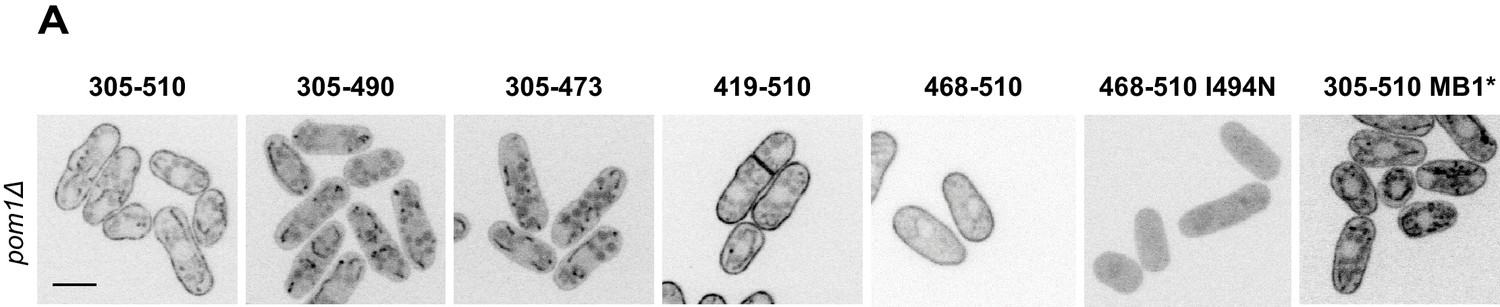
Analysis of Pom1 fragment localization in pom1∆ cells.
Localization in pom1∆ cells of the Pom1 GFP-tagged fragments 1 to 8 presented in Figure 3A. Scale bar 5 μm.
Figure 4 with 1 supplement
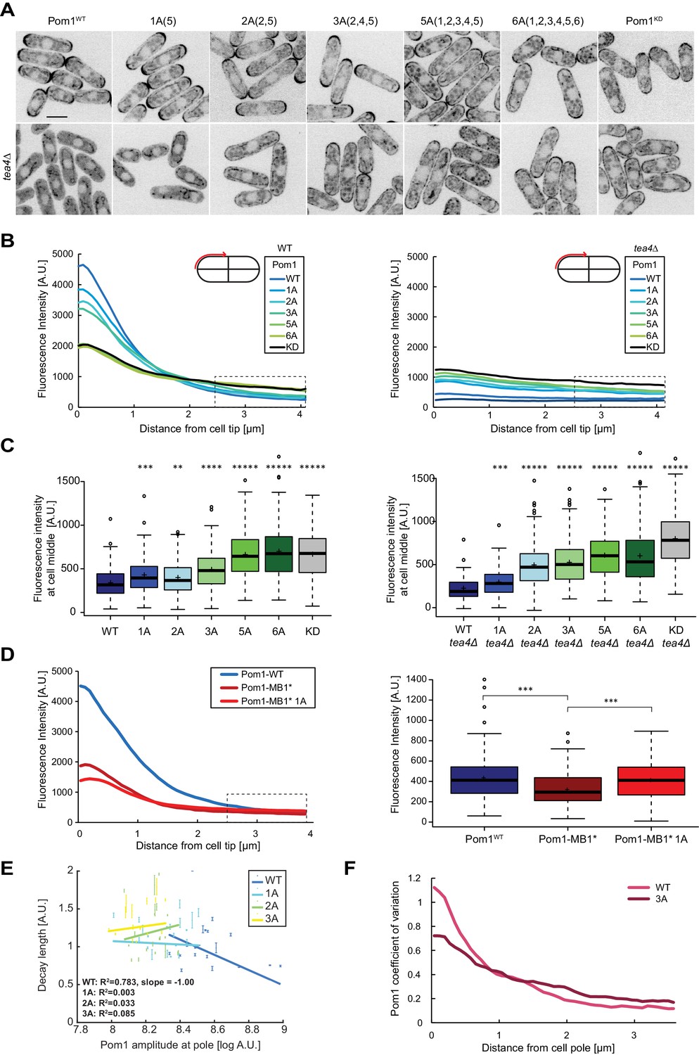
Pom1 gradient shape and robustness depend on multisite auto-phosphorylation.
(A) Medial plane confocal images of a series of Pom1 phospho-blocking alleles in otherwise wild-type (top row) and tea4Δ cells (bottom row). Scale bar 5 μm. (B) Fluorescence intensity plots of cortical gradient profiles, collected from time-average medial plane confocal images as shown on the schematic. Left: wild type background; right: tea4Δ cells. Graphs show averages of 240 gradient profiles per strain, n = 3 experiments, 20 cells per experiment. Individual experiments are shown in Figure 4—figure supplement 1. The dashed box shows the region selected for Pom1 intensity measurements at mid-cell shown in panel C. (C) Mean Pom1 fluorescence intensity levels at cell middle, extracted from the last 1.5 µm of profiles shown in panel B. Left: wild-type background, right: tea4Δ cells. (D) Cortical gradient profiles of Pom1WT, Pom1MB1* and Pom1MB1*-1A(5) (left) and corresponding quantification of Pom1 intensity at cell middle (right), as in panels B and C. Graphs show averages of 160 gradient profiles per strain, n = 2 experiments, 20 cells per experiment. (E) Decay length plotted against Pom1 amplitude at the cell pole. Each dot represents an average gradient profile from bin sorting of 5%. Error bars correspond to the percentage of fitting quality for each dot. (F) Coefficients of variation for Pom1WT and Pom13A from the 240 gradient profiles shown in B. Means indicated by plus sign, error bars: SD, statistical significance measured against wild type unless otherwise indicated by t-test with unequal variances. **, p=0.0001, ***p=10−8, ****p≤10−18, *****p≤10−40.
Figure 4—figure supplement 1
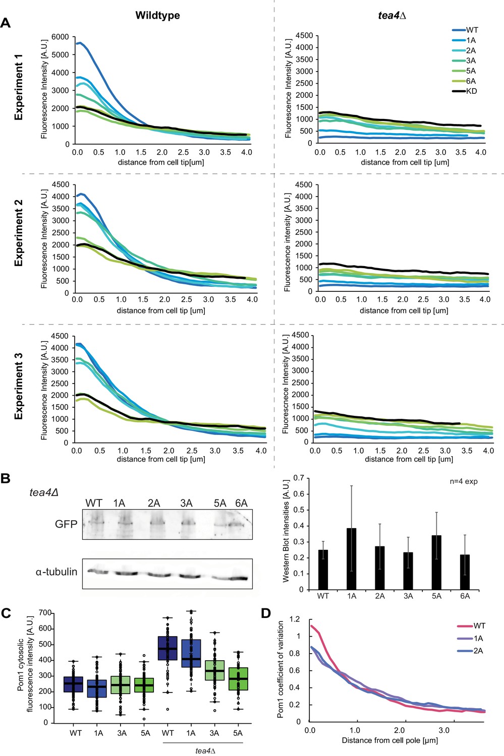
Analysis of Pom1 phospho-site mutant alleles.
(A) Individual experiments for the average fluorescence intensity plots of cortical gradient profiles, collected from time-average medial plane confocal images, shown in Figure 4B. Left: wild-type background; right: tea4Δ cells. Graphs show averages of 80 gradient profiles per strain, collected in 20 individual cells per experiment. (B) Western blot showing equal levels of expression of the various Pom1-GFP alleles in tea4∆ cells, as indicated. α-tubulin was used as a loading control. Average quantification of four experiments is shown on the right. Error bars: standard deviation. (C) Mean Pom1 fluorescence intensity levels in the cytosol in wild-type and tea4Δ cells. (D) Coefficients of variation for Pom1WT, Pom11A, and Pom12A from the gradient profiles shown in Figure 4B.
Figure 5 with 2 supplements
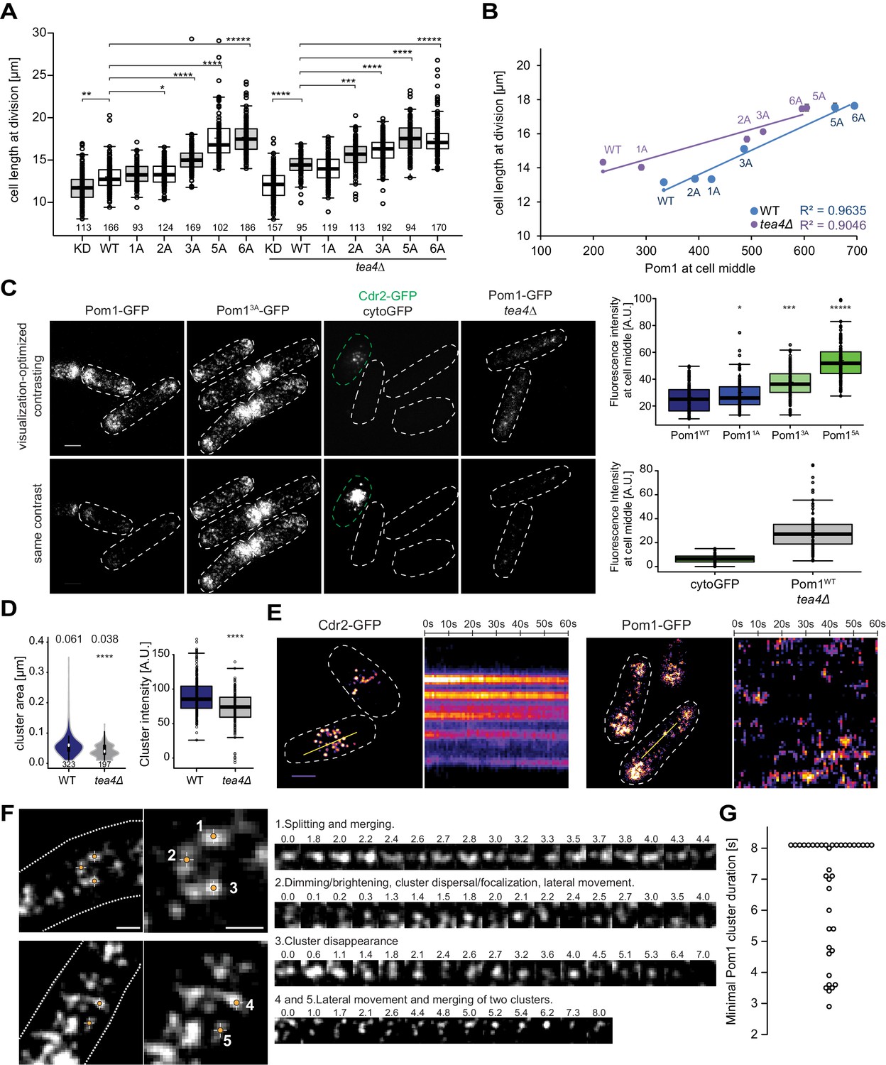
Cortical Pom1 at mid-cell regulates cell size.
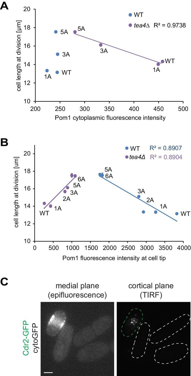
(A) Mean cell length at division of the pom1 phospho-mutant allelic series in otherwise wild type and tea4Δ background with number of quantified cells indicated, *, p=10−2, **, p=10−7, ***, p=10−10, ****, p≤10−20, *****, p=10−40. (B) Correlation plot of cell length at division (values from panel A) versus Pom1 intensity at cell middle (values from Figure 4C). Error bars are standard error. (C) TIRF imaging of Pom1, shown with identical acquisition and contrasting parameters (bottom) and adjusted contrast (top). Quantification of intensities at cell middle is shown on the right (strains imaged the same day plotted together). Pom11A-GFP, Pom13A-GFP and Pom15A-GFP show increased cortical levels compared to Pom1WT-GFP (p=0.01, p=10−14, p=10−41, respectively). Note that cytoGFP expressed from the pom1 promoter strain was mixed with a Cdr2-GFP strain to identify the TIRF focal plane (green dotted line). Scale bar 2.5 μm. Images for Pom11A-GFP and Pom15A-GFP are in supplement 2. (D) Mean cluster area (left) and average cluster intensity (right) for individual Pom1 clusters from wild type versus tea4Δ background, n = 25 cells from two individual experiments. Number of clusters indicated below violin plot. The mean area is shown at the top, ****, p=10−15. (E) Localization of Cdr2-GFP and Pom1-GFP by TIRF microscopy. Left panels show a snapshot of time point 0 from a time series imaged every second for 60 s. Right panels show kymographs along the dotted line. Scale bar 2.5 μm. (F) Examples of Pom1-GFP cluster behaviors in TIRF, taken from two cells imaged every 100 ms over 8 s. Line 1: Cluster splitting (3.0 s and 4.4 s) and merging (3.2 s). Line 2: Cluster fluorescence fluctuations (down at 0.1 s, 2.0 s, 2.4 s; up at 0.2 s, 2.1 s, 2.5 s). This cluster also exhibits clear lateral movement. Line 3: Cluster fluorescence fluctuation (down at 2.4 s and 3.6 s; up at 2.6 s and 4.0 s) and disappearance (7.0 s). Line 4: Merging of two clusters (at 6.2 s). The bottom cluster exhibits clear lateral movement. Scale bars: 1 µm. (G) Minimal lifetimes of Pom1 clusters in seconds. Note that the lifetime of all but two clusters is underestimated, as they either existed at the start or end of the timelapse, or both, n = 38 clusters from 12 cells.
Figure 5—figure supplement 1
Pom1 levels in the cytosol and at cell poles do not correlate with cell length at division.
(A) Correlation plot of cell length at division (values from Figure 5A) versus Pom1 cytosolic levels (values from Figure 4—figure supplement 1C). (B) Correlation plot of cell length at division (values from Figure 5A) versus Pom1 intensity at cell poles (values from Figure 4B). Error bars are standard error. (C) Mid-plane epifluorescence (left) and cortical TIRF (right) images of cytoGFP expressed from the pom1 promoter. Note that the strain was mixed with a Cdr2-GFP strain (green dashed contour) to help find the TIRF focal plane. Scale bar 2.5 μm.
Figure 5—figure supplement 2
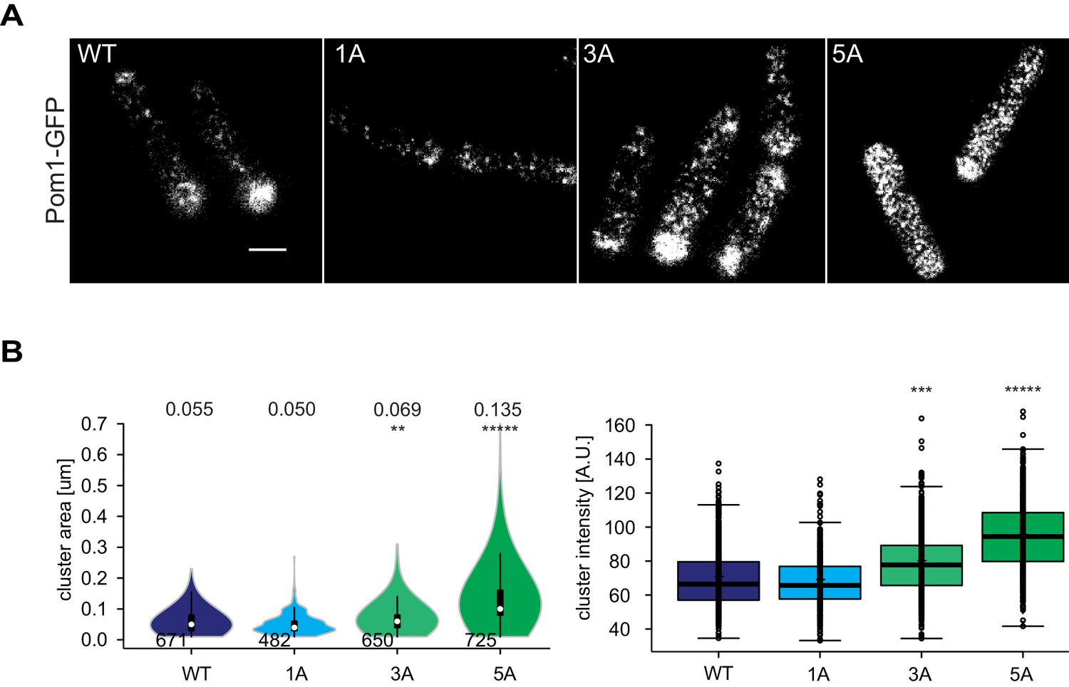
TIRF imaging of Pom11A, Pom13A and Pom15A.
(A) TIRF imaging of Pom1, Pom11A, Pom13A and Pom15A-GFP with identical acquisition and adjusted contrast. Quantification of medial intensities is shown in Figure 5C. Scale bar 2.5 µm. (B) Mean cluster area (left) and intensity (right) for individual Pom1 clusters from Pom1WT, Pom11A, Pom13A and Pom15A background, n = 37 to 42 cells from three individual experiments. Number of clusters indicated below violin plot. The mean area is shown at the top, **, p=10−10, ***, p=10−20, ****, p=10−100.
Figure 6 with 1 supplement
Pom1 levels at Cdr2 nodes are higher in short than long cells.
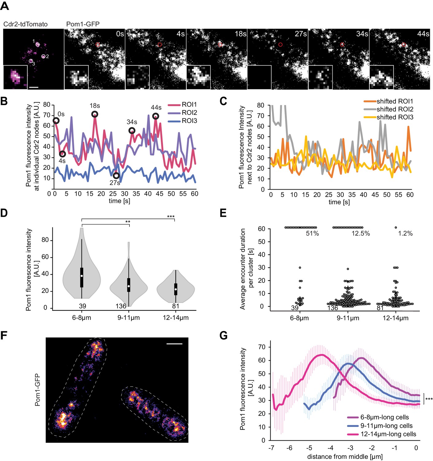
(A) TIRF images of Cdr2-tdTomato and Pom1-GFP in a dual tagged strain. ROIs (1, 2 and 3) were selected around Cdr2 nodes and fluorescence intensity was measured in the GFP channel (ROI one marked in red). Scale bar 1 μm. (B) Pom1-GFP fluorescence intensity in the three ROIs marked in panel A. Circled time points correspond to snapshots in panel A. (C) Pom1-GFP fluorescence intensity in ROIs shifted to the immediate vicinity of the ROIs marked in A. (D) Average fluorescence intensity of Pom1-GFP at Cdr2 nodes measured as in (A–B) over a 60-s imaging period, sorted by cell length. ***, p≤10−7. (E) Duration of individual Pom1 encounters with a Cdr2 node for cells of sorted length. This is defined as the length of time the Pom1-GFP signal is over 20 arbitrary fluorescence units. In longer cells, the proportion of clusters with continuous (60 s) Pom1 presence decreases, while the number of shorter encounters increases. For (D–E), data was collected from a single experiment: 39 clusters from 6 6–8 μm long cells, 136 clusters from 21 9–11 μm long cells, and 81 clusters from 13 12–14 μm long cells. Experiment duplicates presented in Figure 6—figure supplement 1. (F) Localization of Pom1-GFP in TIRF in cells of different lengths (10 μm and 13.5 μm). Scale bar 2.5 µm. (G) Global cortical Pom1 levels measured from TIRF imaging. The gradients are aligned to the cell geometric middle and sorted by cell length. Error bars: standard error between experiments (N = 3); in total 62 gradients from 6 to 8 μm cells, 248 gradients from 9 to 11 μm cells and 128 gradients from 12 to 14 μm cells. Statistics on Pom1 medial levels performed for the last 1.5 μm of the gradient tail between short (6–8 μm) and intermediate cells (9–11 μm), p=10−3, and between short and long cells (12–14 μm), p=10−6.
Figure 6—figure supplement 1

Replicate experiments showing higher Pom1-GFP fluorescence at Cdr2 nodes of short than long cells.
(A-B) Fluorescence intensity of Pom1-GFP at Cdr2 nodes measured as in Figure 6B every second over a 60-s imaging period (A) or every 100 ms over an 8-s imaging period (B), sorted by cell length. **, p=10−3, ***, p≤10−05, ****, p≤10−15. (C) Duration of individual Pom1 encounters with a Cdr2 node for cells of sorted length, measured as in Figure 6E. Note that 50 arbitrary units were chosen to define Pom1-GFP presence at a Cdr2 node. For experiment 2, the data was collected on the same day: for the one frame/s acquisition 29 clusters from 7 6–8 μm long cells, 115 clusters from 15 9–11 μm long cells, and 64 clusters from 8 12–14 μm long cells were quantified; for the 100 ms interval acquisition, 26 clusters from 6 6–8 μm long cells, 36 clusters from 7 9–11 μm long cells, and 60 clusters from 6 12–14 μm long cells were quantified. For experiment 3, the data was collected on the same day: for the one frame/s acquisition 97 clusters from 16 6–8 μm long cells, 230 clusters from 27 9–11 μm long cells, and 62 clusters from 6 12–14 μm long cells were quantified; for the 100 ms interval acquisition 74 clusters from 14 6–8 μm long cells, 190 clusters from 22 9–11 μm long cells, and 80 clusters from 12 12–14 μm long cells were quantified.
Author response image 1

Videos
Video 1
Examples of Pom1-GFP cluster dynamics.
Pom1-GFP was imaged in TIRF mode every 100 ms over a 8 s imaging period. 4 clusters of interest are marked with a target with three prominent clusters visible at the start of the timelapse, and one smaller cluster at the bottom of the frame which appears at 0.2 s and disappears temporarily at 1.2 s and 1.8 s and completely at 5.6 s (possibly as it leaves the evanescent field on the side of the cell). The top positioned cluster splits at 2.8 s (or even sooner), remerges at 3.3 s, splits partially at 3.7 s and completely at 4.4 s, leaving behind two smaller clusters that move laterally and last until the end of the movie. The bottom cluster on at timepoint 0 is observed clearly until 6.9 s. During this period, it dims and brightens, disperses and focalizes several times. At 6.9 s disappears from the field of view, but may not be completely absent as a cluster (not marked) reappears at the same location at 7.0 s. The cluster on the left moves laterally and splits in two clusters at 2.2 s and re-merges at 2.7 s and remains trackable until the end of the 8 s imaging period. All clusters tracked in this movie show examples of dimming, followed by brightening of the signal. The movie is shown in quasi-real time.
Video 2
Examples of Pom1-GFP cluster dynamics.
Pom1-GFP was imaged in TIRF mode every 100 ms over a 8-s imaging period. Three clusters of interest are marked with a target. The cluster on the left- splits in three smaller clusters at 0.1 s, after which the clusters appear to detach. The cluster on the top right splits in two clusters at 0.1 s and re-merges briefly at 0.2 s, after which the cluster increases in brightness and splits again at 0.6 s. The small cluster on the left moves laterally, dims in fluorescence and eventually detaches at 1.3 s. The right top cluster and the bottom cluster, marked from the beginning of the movie move laterally, occasionally splitting and merging. The top cluster splits at 2.4 s and re-merges at 2.7 s, as does the bottom cluster at 3.2 s and 3.4 s, and 4.5 s. Eventually, the clusters will merge at 4.9 s, forming a bright and stable cluster, which remains trackable until the end of the 8-s imaging period. The movie is shown in quasi-real time.
Video 3
Examples of Pom13A-GFP cluster dynamics.
Pom13A-GFP was imaged in TIRF mode every 100 ms over an 8-s imaging period. Four clusters of interest are marked with a target. The two clusters on the bottom left are short-lived. The top cluster dims at 0.7 s, increases in brightness at 1.1 s and disappears at 1.7 s. The neighbouring small clusters disappear at 0.3 s and 0.9 s. The top two clusters are longer lived with the top cluster dimming at 7.1 s and increasing in brightness at 7.3 s, remaining trackable until the end of the 8-s imaging period, while the lower cluster displays lateral movements between 5.8 s to 6.3 s, dims at 6.5 s and disappears at 6.6 s. The movie is shown in quasi-real time.
Video 4
Examples of Pom15A-GFP cluster dynamics.
Pom15A-GFP was imaged in TIRF mode every 100 ms over an 8-s imaging period. Three main areas of interest are marked with targets. The top cluster displays lateral movements between 2.5 s and 3.1 s and disappears at 3.3 s. The middle area tracks three smaller highly dynamic clusters, displaying merging (2.7 s and 4.3 s) and splitting events (3.0 s). The fused cluster shows increase of brightness at 4.4 s and disappears at 7.0 s. The bottom cluster is trackable throughout the imaging period and shows dimming and increase of brightness between 5.8 s and 5.9 s. The movie is shown in quasi-real time.
Additional files
-
Supplementary file 1
S. pombe strains used in this study.
- https://doi.org/10.7554/eLife.45983.024
-
Supplementary file 2
Plasmid used in this study.
- https://doi.org/10.7554/eLife.45983.025
-
Supplementary file 3
Primers used for mutagenesis.
Bold residues indicate changes from the wildtype sequence.
- https://doi.org/10.7554/eLife.45983.026
-
Supplementary file 4
Global fitting parameters and outputs for diffusion and dissociation coefficients.
- https://doi.org/10.7554/eLife.45983.027
-
Source code 1
MATLAB script for decay length analysis of wild type, Pom11A, Pom12A, and Pom13A gradients provided with raw data files for each condition.
- https://doi.org/10.7554/eLife.45983.023
-
Transparent reporting form
- https://doi.org/10.7554/eLife.45983.028
Download links
A two-part list of links to download the article, or parts of the article, in various formats.
Downloads (link to download the article as PDF)
Open citations (links to open the citations from this article in various online reference manager services)
Cite this article (links to download the citations from this article in formats compatible with various reference manager tools)
Multi-phosphorylation reaction and clustering tune Pom1 gradient mid-cell levels according to cell size
eLife 8:e45983.
https://doi.org/10.7554/eLife.45983


