Structural principles of SNARE complex recognition by the AAA+ protein NSF
- Stanford University, United States
- Howard Hughes Medical Institute, Stanford University, United States
- University of Chicago, United States
Figures
Figure 1 with 3 supplements

Flowchart of data processing.
After initial 2D classification, 475,680 particles were selected for 3D classification. Two out of the resulting four classes show significantly better features (Classes II and IV). Class IV shows clear density for N domains, SNARE complex, and αSNAP, while these features are weaker—but still present— in the case of Class II. Two refinement paths were thus taken (Materials and methods). The first path combined the two classes and focused on NSF, yielding two maps at 3.9 Å and 3.8 Å with different conformations at the pore loops. The second path focused on Class IV, which yielded two maps at 4.4 Å with different conformations for the SNARE and αSNAP subcomplex.
Figure 1—figure supplement 1
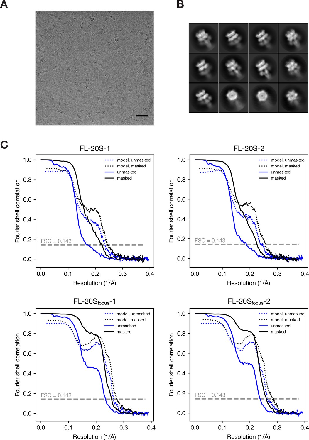
Representative data and resolution estimation for single particle analysis.
(A) Representative electron micrograph of the 20S supercomplex after motion correction. Scale bar corresponds to 50 nm. (B) Selected 2D class averages showing side views and end-on views. (C) FSC curves for the masked and unmasked 3D density maps after RELION post-processing as well as FSC curves calculated with masked and unmasked maps against the final models. The resolution for each is estimated by the FSC = 0.143 criterion; see Table 1 for values.
Figure 1—figure supplement 2

3D density maps for (A) FL-20S-1, (B) FL-20S-2, (C) FL-20Sfocus-1, and (D) FL-20Sfocus-2 colored according to local resolution as calculated by ResMap (Kucukelbir et al., 2014).
https://doi.org/10.7554/eLife.38888.004
Figure 1—figure supplement 3
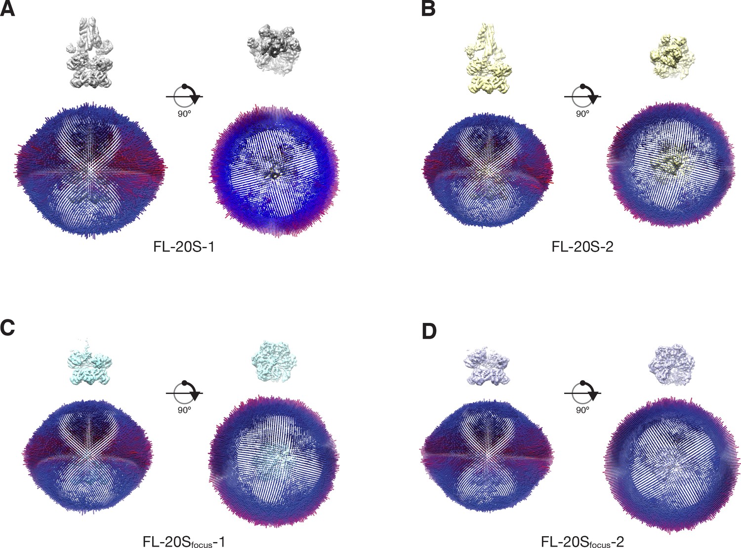
Plots of angular distributions for each of the 20S classes perpendicular to and along the NSF pore axis (A–D).
The length and color of each cylinder is proportional to the number of particle images observed at that angle. Maps are shown for reference, contoured at 4.8 σ. A slight bias for views perpendicular to the pore axis (‘side views’) is present for all classes, consistent with previous observations (Zhao et al., 2015).
Figure 2

Representative density for various features from the FL-NSFfocus-1 class, contoured at 4.8 σ.
(A) The α2 helix and pore loop of the protomer B D1 domain, with residues 290 – 320 shown. (B) The parallel β sheet from the protomer B D1 domain, composed of β strands 1 – 5. (C) The presence of the first 17 residues of SNAP-25A is supported by the FL-20Sfocus-1 density. Density is strongest for residues in the pore of NSF, while the first two N-terminal residues and residues beyond the C-terminus of R17 appear more conformationally heterogeneous.
Figure 3 with 1 supplement

Architecture of the 20S complex, composed of NSF (N domains, salmon; D1 domains, cyan; D2 domains, purple), αSNAPs (gold), and the neuronal SNARE complex (syntaxin-1A, red; synaptobrevin-2, blue; SNAP-25A, green).
(A) Sharpened FL-20S-1 map contoured at 4.8 σ; N domains for NSF subunits A–D are visible at this threshold. (B) FL-20S-1 composite model, with nucleotides represented by yellow spheres. (C) The pattern of N domain engagement with the αSNAP/SNARE complex varies between the FL-20S-1 and FL-20S-2 classes; in the second class, the pattern of engagement shifts one protomer counter-clockwise about the hexamer axis. The bottom panels show schemas of the configurations. Despite changes in spire architecture, the split in the D1 ring is found between protomers A and F in both classes, with protomer A furthest from the viewer.
Figure 3—figure supplement 1
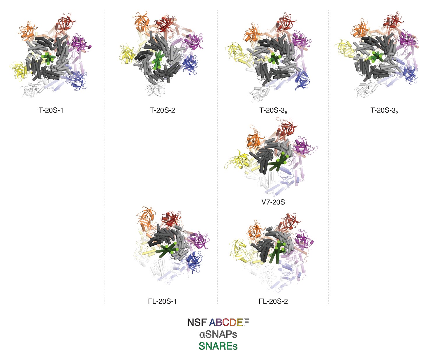
Comparison of NSF N domain engagement with αSNAPs and different SNARE complexes.
Known engagement patterns are sorted by column. Truncated (T-20S) and V7 (V7-20S) 20S models published (Zhao et al., 2015) are shown on the first two rows, and the full length (FL-20S) structures are shown in the third row. The engagement pattern of FL-20S-1 most closely resembles T-20S-2, while the engagement pattern of FL-20S-2 is most similar to T-20S-3 and V7-20S.
Figure 4
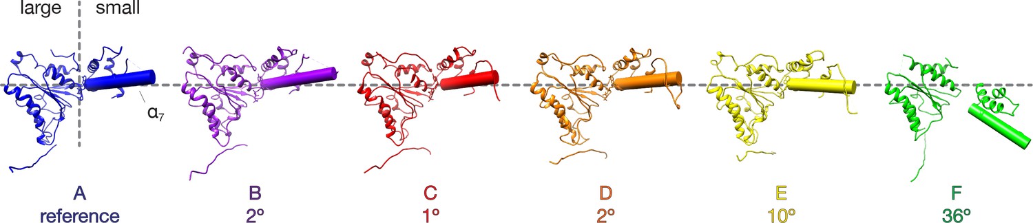
Comparison of NSF D1 small subdomain conformations in the FL-20S-1 model.
The large D1 subdomains of all protomers were superimposed, and angles were calculated between the small subdomain α7 helical axes of protomer A and protomers B-F. Superposition was performed on the large subdomain due to improved alignment. Protomers E and F show substantial angular deviations in comparison to the domains A-D, consistent with remodeling of the hinge region between the large and small subdomains.
Figure 5
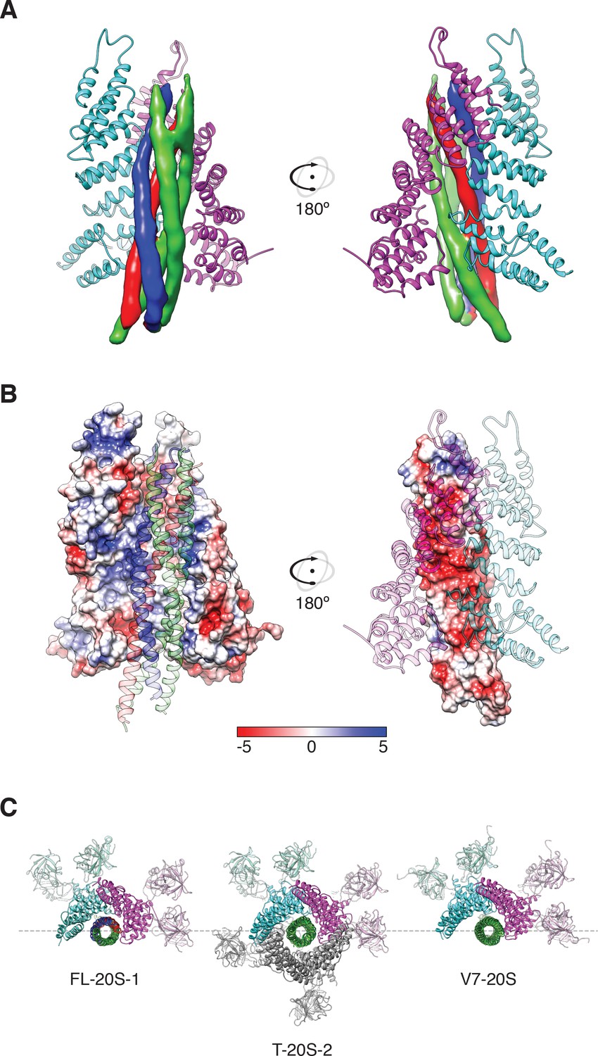
Two αSNAP molecules (blue, magenta) bind the full-length neuronal SNARE complex composed of SNAP-25A (green), syntaxin-1A (red), and synaptobrevin-2 (blue) at a well-defined orientation.
(A) Reconstructed density for the neuronal SNARE complex in the FL-20S-1 map, contoured at 7.1 σ. (B) Electrostatic surfaces for the αSNAPs (left) and SNARE complex (right) reveal a complementary pattern of positive and negative charge, respectively. Calculations were performed using APBS assuming 150 mM NaCl, with units in kT. (C) Comparison of N domain and αSNAP stoichiometry for the full-length (FL-20S-1) and truncated (T-20S-2) reconstructions as well as for the V7-20S reconstruction; T-20S-2 is the only complex to show four αSNAPs bound to the SNARE complex.
Figure 6
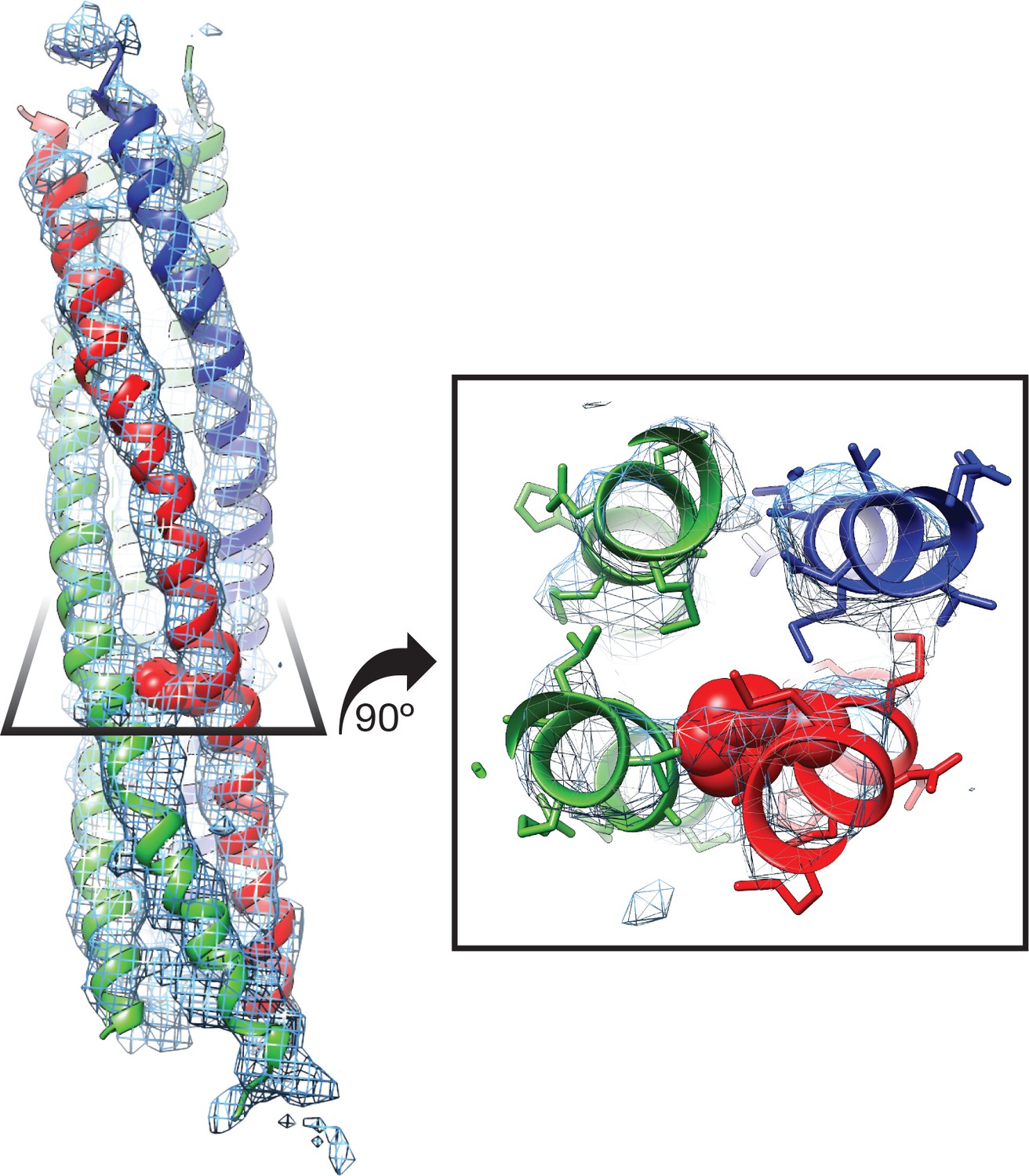
Side chain density at −3 layer corresponding to syntaxin-1A F216 supports SNARE complex orientation.
SNAP-25A (green), syntaxin-1A (red), and synaptobrevin-2 (blue) are shown with representative density from the FL-20S-1 reconstruction, contoured at 5.5 σ. F216 is shown as spheres, while nearby side chains are depicted as sticks.
Figure 7
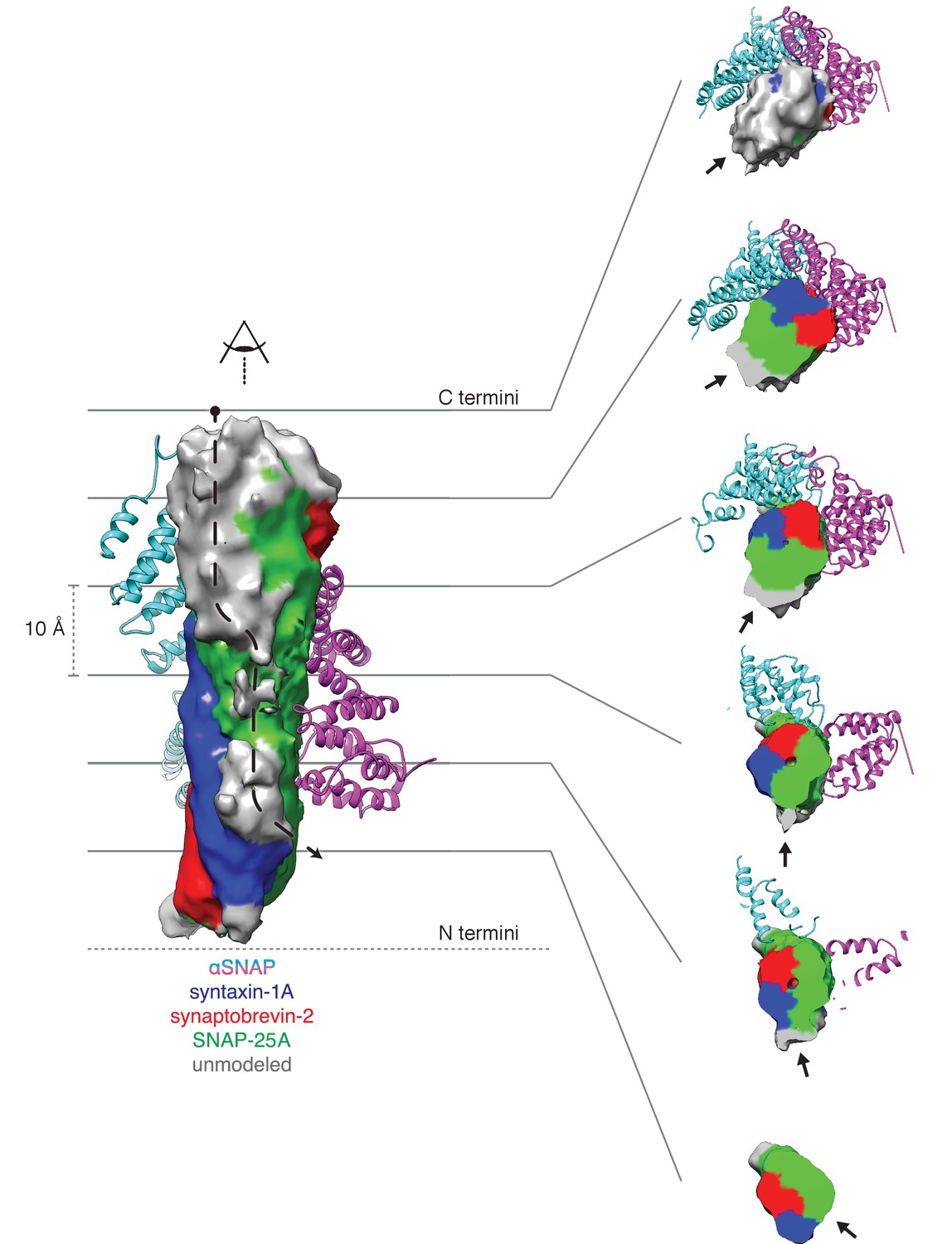
Density running along the solvent-exposed face of the SNARE complex is consistent with the presence of the linker that connects the two SNAP-25A SNARE motifs.
Surfaces are contoured at 2 σ and colored based on the identity of the nearest atom within 5 Å; green corresponds to SNAP-25A, blue to synaptobrevin-2, and red to syntaxin-1A. Grey surfaces indicate a surface further than 5 Å from any modelled atom. The two αSNAP molecules are depicted in cyan and magenta. The portion of the linker corresponding to the unmodeled density at the top C-terminal end (i.e., the membrane proximal region) of the SNARE complex includes four cysteines which are palmitoylated in vivo (Greaves et al., 2009; Hess et al., 1992); this modification promotes association with the plasma membrane during trafficking and enhances its association at the presynaptic membrane. A possible path from N- to C-terminal end of the linker is indicated by a dashed arrow (left). This path is also shown as a series of slices through the complex (right), with an arrow indicating the putative linker density. The relatively weak and diffuse density suggests that the linker is flexible and present in multiple conformations.
Figure 8
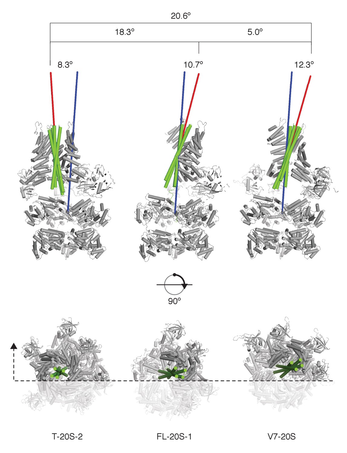
SNARE complex orientation varies across constructs.
The D1 domains of T-20S-2, FL-20S-1, and V7-20S structures were used to superimpose the rest of each model. SNARE complexes (green) are shown in green relative to the rest of each 20S complex (grey), with the viewing plane slicing through the center of the complex as indicated by a dashed line. Principle axes for each independent SNARE complex (red) and for all D1 domains (blue) are drawn, projecting out from the center of mass of each. The distances between the D1 center of mass and the SNARE complex center of mass, distances between the different SNARE complex centers of mass, angles between SNARE complex principle vectors and the D1 principle vector, and the angles between different SNARE complex principle vectors are shown.
Figure 9 with 1 supplement
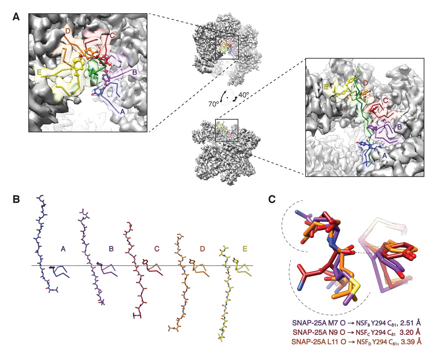
The NSF D1 pore loops guide the SNAP-25A N-terminus through the pore.
(A) The FL-20Sfocus-1 map, contoured at 4.8 σ, with the SNAP-25A N-terminus and NSF D1 pore loops shown in cartoon format, color coded by protomer. The Y294 side chains are shown as well. The NSF D1 pore loops form a spiral pattern of interactions with the substrate, wherein Y294 interacts with every other substrate residue. The final pore loop from protomer F disengaged. (B) Sequential engagement of SNAP-25A by NSF D1 pore loops on protomers A–E. Full side chains are omitted from the SNAP-25A for clarity. The D1 domains of protomers A–E were superimposed, revealing conformational changes in the pore loops themselves. Protomer A and E pore loops are less directly engaged with substrate, with the protomer A relatively closer to the SNAP-25A N-terminus than expected by symmetry. (C) Overlay of the D1 domain pore loops of protomers B–D reveal a set of stereotyped interactions between each Y294 Cδ1 and the carbonyl of SNAP-25A residue 7, 9, or 11, respectively. Side chains are positioned away from the intercalation point (dashed lines).
Figure 9—figure supplement 1
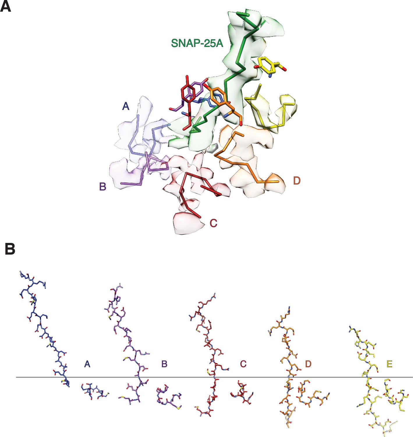
The secondary NSF D1 domain pore loops (residues 338–345) guide the N-terminus of SNAP-25A through the pore.
(A) Off-axis view through the NSF D1 pore towards the N-terminus of SNAP-25A with sharpened density contoured at 4 σ and segmented around substrate and secondary loop residues. The peptide backbones of substrate and the secondary pore loops are shown for clarity, and the Y294 side chain from the primary D1 pore loop is shown for reference. The substrate is tightly engaged by Y294, but the secondary pore loops do not form any stereotyped interactions with it. The quality of the map varies substantially for each subunit, and no specific interaction with substrate is evident. (B) Sequential interaction of secondary pore loops A-E with substrate. As expected, secondary pore loops are closer to substrate in the protomers closest to the entry of the pore and furthest from the D2 ring.
Figure 10 with 1 supplement
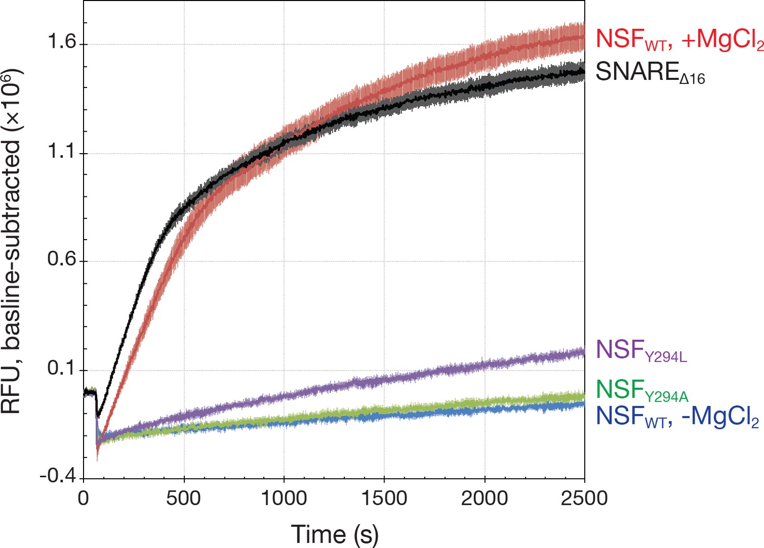
Kinetics traces measured using a fluorescence dequenching assay reveal the effects of pore loop mutations and the truncation of the 16 SNAP-25A N-terminal residues (SNAREΔ16) on disassembly activity.
Wild-type αSNAP was used throughout. For pore loop mutations and wild type controls, full-length soluble SNARE complex labeled with Oregon Green 488 was used as substrate. For testing disassembly of the SNAREΔ16 complex, wild type NSF was used. All reactions were triggered with the addition of MgCl₂. Each curve is the average of five or six replicates; error bars represent standard error about the mean. Mutation of Y294 reduces disassembly rate, while truncation of the SNAP-25A N-terminal residues increases it slightly.
Figure 10—figure supplement 1
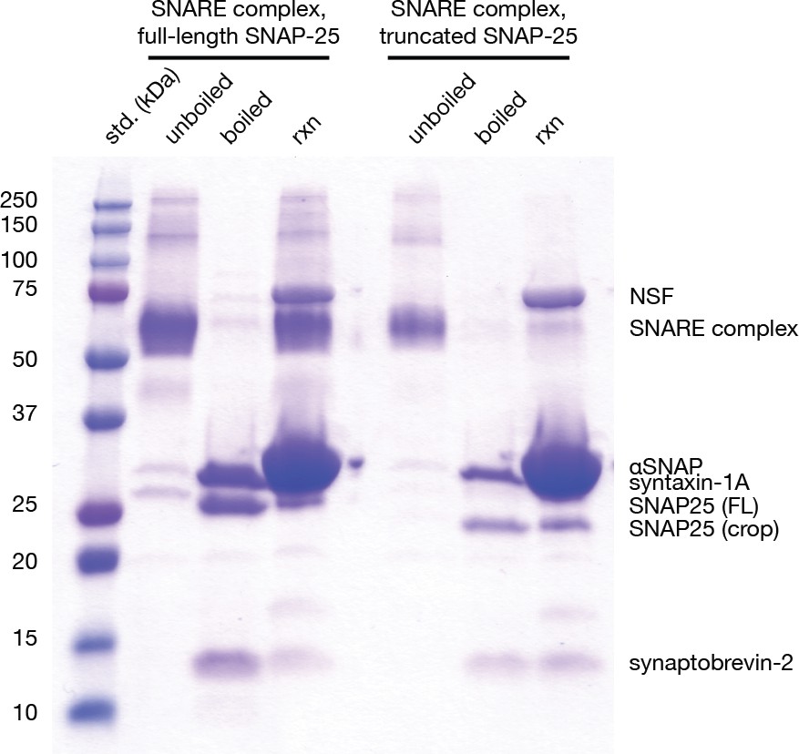
Gel-based assay for disassembly of full-length neuronal SNARE complex and the truncated neuronal SNARE complex composed of full-length syntaxin-1A, synaptobrevin-2, and SNAP-25AΔ16.
Unboiled lanes show assembled neuronal SNARE complexes of the appropriate size (full-length, 65221 kDa; truncated, 63,397 kDa). Boiling the SNARE complexes leads to complete disassembly, and each resulting band represents an individual SNARE protein (syntaxin-1a, 30.726 kDa; synaptobrevin-2, 10.870 kDa; SNAP-25A, 23.625 kDa, SNAP-25AΔ16, 21.801 kDa). A shift in electrophoretic mobility is visible SNAP-25A and SNAP-25AΔ16. Further addition of NSF (82.802 kDa per monomer) and αSNAP (33.250 kDa) to a final NSF:αSNAP:SNARE complex ratio of 0.05:5:1 for full-length SNARE complex and 0.1:10:1 for truncated SNARE complex in the presence of 25 mM Tris pH 8, 2 mM ATP, and 4 mM MgCl2 for 5 min at 37°C leads to disassembly of the SNARE complexes at similar rates as judged by the intensity of individual SNARE protein bands.
Figure 11 with 1 supplement
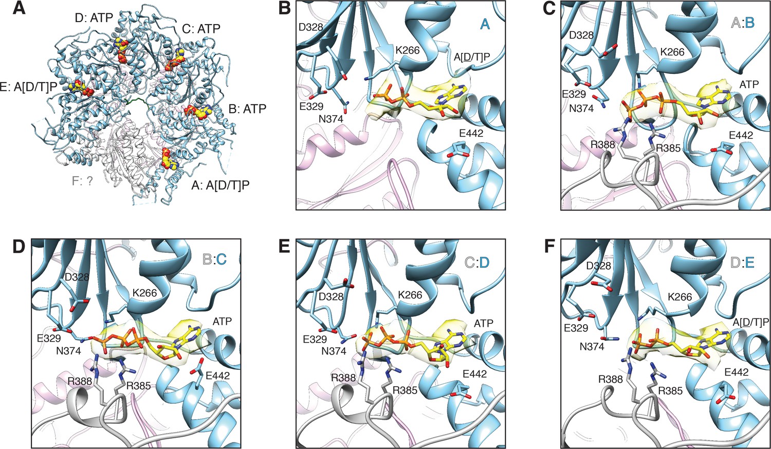
FL-20Sfocus-1 D1 domain nucleotide state varies as a function of protomer identity.
(A) Overview of the D1 ring nucleotide state. D1 domains of protomers B–D (blue) bind ATP while the D1 domains of protomers A and E show ambiguous density. The D1 domain of protomer F from the ATP-bound structure of substrate-free NSF (white) was placed by superposition of D1 rings. Substrate (green), and the D2 ring (purple) are shown for reference. (B–F) Nucleotide (yellow) and the nucleotide binding site are shown for each D1 domain. The preceding D1 protomer is also shown (grey). Nucleotide density is contoured at 4.8 σ. In each case, the Walker A motif (p-loop; residues 260–267, including K266) largely coordinates binding. A pair of arginine side chains (R385, R388) from the preceding protomer serve as the arginine fingers and contribute to nucleotide coordination as well. Several essential residues from sensor 1 (N374) and 2 (E442) motifs are also shown. The acidic residues of the Walker B motif (residues D328 and E329 from residues 324–329) are disengaged from the active site in the absence of a magnesium ion.
Figure 11—figure supplement 1
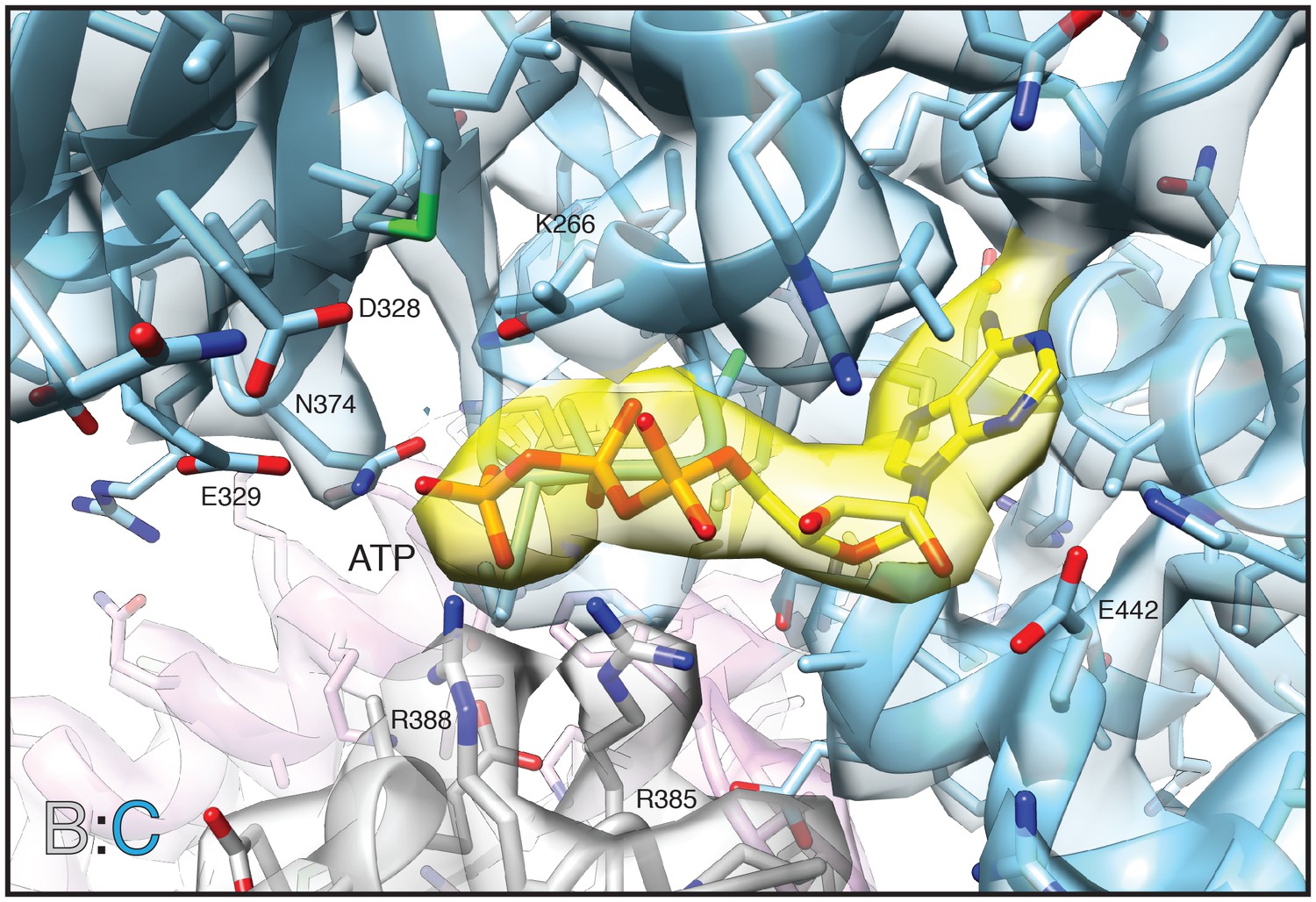
Non-segmented density and corresponding model of the D1 nucleotide binding pocket (blue) and bound ATP (yellow) for protomer C from the FL-20Sfocus-1 class reconstruction.
Arginine fingers (R385, R388) from protomer B (grey) interact with the nucleotide. Other key residues are labeled. The sharpened map is contoured at 7.5 σ.
Figure 12
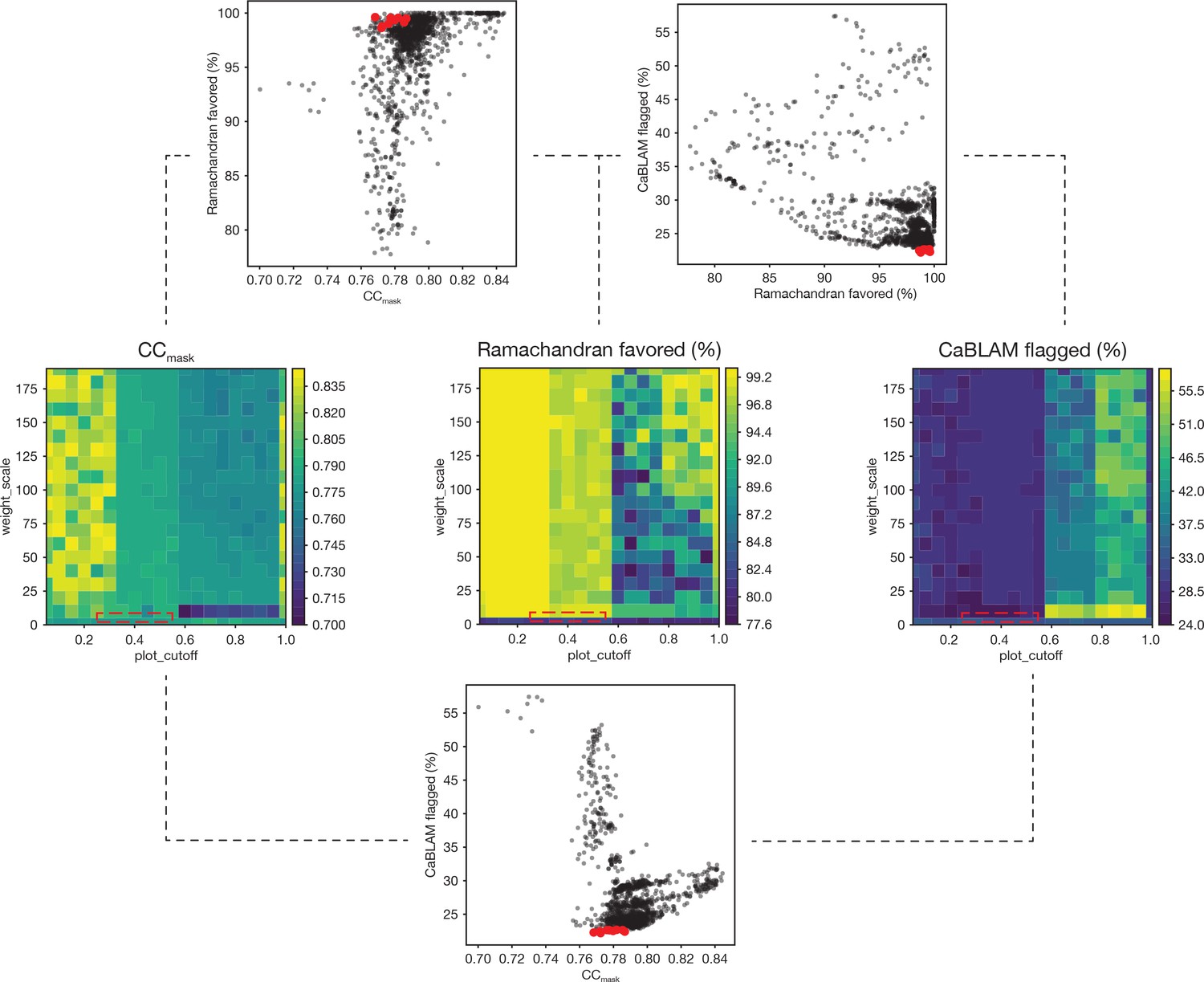
Summary of a 1,306-point refinement grid search.
CaBLAM scores were used to guide the enforcement of Ramachandran restraints. At several points during the iterative refinement of the final FL-20Sfocus models, Ramachandran restraints were imposed using the Oldfield target function (Oldfield, 2001) as implemented in phenix.real_space_refine (Adams et al., 2010; Headd et al., 2012). A grid of refinements with different values of the parameters weight_scale and plot_cutoff were performed; the results are visualized as surfaces for three key diagnostic parameters—CCmask, Ramachandran fraction favored, and the total fraction of residues flagged by CaBLAM analysis (i.e., the total fraction of residues flagged as either outliers, disfavored, or severe) (Richardson et al., 2018). The value of plot_cutoff largely sorts results into three matching regions for each metric, while the value of weight_scale is less predictive. The ten refinements with the lowest CaBLAM scores were further examined, and one model was chosen for subsequent manual and automated refinement. The boxes (dashed lines) on the surface plots illustrate the regions from which these models were found in parameter space. Scatter plots reveal the relationships between CCmask, Ramachandran fraction favored, and CaBLAM fraction flagged; the top ten refinements as identified by CaBLAM are shown (red points).
Tables
Table 1
Refinement statistics for each reconstruction and model.
https://doi.org/10.7554/eLife.38888.007| FL-20S-1 | FL-20S-2 | FL-20Sfocus-1 | FL-20Sfocus-2 | |
|---|---|---|---|---|
| Data acquisition: | ||||
| Microscope | FEI Titan Krios | FEI Titan Krios | FEI Titan Krios | FEI Titan Krios |
| Detector | Gatan K2 Summit | Gatan K2 Summit | Gatan K2 Summit | Gatan K2 Summit |
| Voltage (keV) | 300 | 300 | 300 | 300 |
| Electron dose (e- Å-2) | 58 | 58 | 58 | 58 |
| Dose rate (e- sec-1 px-1) | 10 | 10 | 10 | 10 |
| Pixel size (Å) | 1.31 | 1.31 | 1.31 | 1.31 |
| Defocus range (µm) | 1.5–3.0 | 1.5–3.0 | 1.5–3.0 | 1.5–3.0 |
| Refined particles | 475680 | 475680 | 475680 | 475680 |
| Reconstruction: | ||||
| Final particles | 166620 | 184555 | 55150 | 62723 |
| Resolution (masked): | ||||
| FSC, 0.5 (Å) | 6.3 | 6.0 | 4.4 | 4.2 |
| FSC, 0.143 (Å) | 4.4 | 4.4 | 3.9 | 3.8 |
| Resolution (unmasked): | ||||
| FSC, 0.5 (Å) | 7.5 | 7.3 | 6.1 | 5.7 |
| FSC, 0.143 (Å) | 5.8 | 5.3 | 4.2 | 4.2 |
| Sharpening B-factor (Å2) | –178.83 | –181.52 | –151.16 | –150.50 |
| Model composition: | ||||
| Total atoms | 73313 | 73052 | 45507 | 45348 |
| Peptide chains | 11 | 11 | 7 | 7 |
| Protein residues | 4662 | 4643 | 2854 | 2843 |
| Refinement: | ||||
| Unit cell | P1 | P1 | P1 | P1 |
| a, b, c (Å) | 301.30, 301.30, 301.30 | 163.75, 146.72, 227.94 | 145.41, 137.55, 117.9 | 301.30, 301.30, 301.30 |
| α = β = γ (º) | 90 | 90 | 90 | 90 |
| CCmask | 0.77 | 0.77 | 0.80 | 0.78 |
| Resolution (vs. model, masked): | ||||
| FSC, 0.5 (Å) | 5.9 | 4.8 | 4.0 | 4.0 |
| FSC, 0.143 (Å) | 4.1 | 3.9 | 3.6 | 3.5 |
| Resolution (vs. model, unmasked): | ||||
| FSC, 0.5 (Å) | 7.0 | 6.8 | 4.3 | 4.3 |
| FSC, 0.143 (Å) | 4.3 | 4.2 | 3.8 | 3.8 |
| RMS Deviations: | ||||
| Bond lengths (Å) | 0.010 | 0.016 | 0.015 | 0.009 |
| Bond angles (º) | 1.337 | 1.77 | 1.52 | 1.53 |
| Ramachandran statistics: | ||||
| Favored (%) | 95.82 | 96.94 | 99.65 | 97.51 |
| Allowed (%) | 3.90 | 2.82 | 0.31 | 2.16 |
| Outliers (%) | 0.28 | 0.24 | 0.04 | 0.33 |
| Validation: | ||||
| Rotamer outliers (%) | 0.10 | 0.36 | 0.16 | 0.33 |
| All-atom clashscore | 4.75 | 6.63 | 6.69 | 5.27 |
| EMRinger score | 0.51 | 0.52 | 1.91 | 1.39 |
| MolProbity score | 1.53 | 1.55 | 1.37 | 1.38 |
Table 2
Refinement statistics for the ten models out of 1306 with the lowest fraction of residues flagged by CaBLAM (see Figure 12).
The model corresponding to plot_cutoff = 0.30 and weight_scale = 2.51 (row highlighted in red) was chosen for further rounds of refinement based on good overall geometry and a minimal number of twisted residues.
| Oldfield plot_ cutoff | Oldfield weight_ scale | CaBLAM flagged (%) | CCmask | Clashscore | Bonds RMSD (Å) | Angles RMSD (º) | Ramachandran outliers (%) | Ramachandran allowed (%) | Ramachandran favored (%) | Rotamer outliers (%) | cis- general (%) | twisted general (%) | Chirality RMSD | Dihedral RMSD (º) |
|---|---|---|---|---|---|---|---|---|---|---|---|---|---|---|
| 0.30 | 4.21 | 17.38 | 0.769 | 3.26 | 0.005 | 1.068 | 0 | 0.31 | 99.69 | 0.12 | 0 | 2.00 | 0.089 | 12.159 |
| 0.30 | 3.71 | 17.58 | 0.765 | 3.09 | 0.004 | 1.064 | 0 | 0.27 | 99.73 | 0.16 | 0 | 2.03 | 0.088 | 12.322 |
| 0.20 | 5.21 | 17.64 | 0.773 | 3 | 0.006 | 1.066 | 0 | 0.24 | 99.76 | 0.12 | 0 | 1.35 | 0.09 | 12.253 |
| 0.25 | 4.31 | 17.71 | 0.778 | 3.43 | 0.007 | 1.102 | 0 | 0.45 | 99.55 | 0.12 | 0 | 1.64 | 0.091 | 12.498 |
| 0.30 | 3.81 | 17.75 | 0.774 | 3.58 | 0.006 | 1.085 | 0 | 0.41 | 99.59 | 0.16 | 0 | 1.93 | 0.09 | 12.44 |
| 0.30 | 5.21 | 17.85 | 0.791 | 3.85 | 0.012 | 1.283 | 0 | 0.45 | 99.55 | 0.36 | 0 | 2.50 | 0.105 | 13.306 |
| 0.30 | 4.31 | 17.88 | 0.788 | 3.83 | 0.011 | 1.247 | 0 | 0.52 | 99.48 | 0.16 | 0 | 2.14 | 0.102 | 13.096 |
| 0.25 | 4.91 | 17.91 | 0.783 | 3.73 | 0.008 | 1.14 | 0 | 0.38 | 99.62 | 0.16 | 0 | 1.82 | 0.094 | 12.795 |
| 0.25 | 4.21 | 17.91 | 0.785 | 3.66 | 0.01 | 1.174 | 0 | 0.45 | 99.55 | 0.08 | 0 | 1.64 | 0.096 | 12.712 |
| 0.20 | 7.11 | 17.91 | 0.776 | 3.45 | 0.006 | 1.095 | 0 | 0.1 | 99.9 | 0.16 | 0 | 1.75 | 0.091 | 12.258 |
Additional files
-
Transparent reporting form
- https://doi.org/10.7554/eLife.38888.023
Download links
A two-part list of links to download the article, or parts of the article, in various formats.
Downloads (link to download the article as PDF)
Open citations (links to open the citations from this article in various online reference manager services)
Cite this article (links to download the citations from this article in formats compatible with various reference manager tools)
Structural principles of SNARE complex recognition by the AAA+ protein NSF
eLife 7:e38888.
https://doi.org/10.7554/eLife.38888


