Ongoing, rational calibration of reward-driven perceptual biases
- University of Pennsylvania, United States
Figures
Figure 1
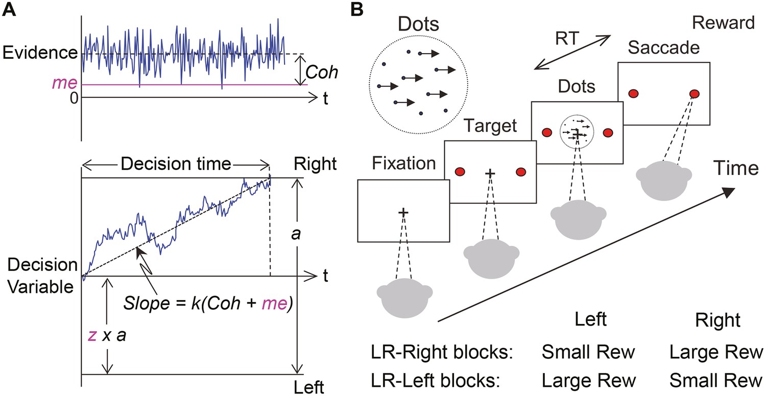
Theoretical framework and task design.
(A) Schematics of the drift-diffusion model (DDM). Motion evidence is modeled as samples from a unit-variance Gaussian distribution (mean: signed coherence, Coh). Effective evidence is modeled as the sum of motion evidence and an internal momentary-evidence bias (me). The decision variable starts at value a × z, where z governs decision-rule bias and accumulates effective evidence over time with a proportional scaling factor (k). A decision is made when the decision variable reaches either bound. Response time (RT) is assumed to be the sum of the decision time and a saccade-specific non-decision time. (B) Response-time (RT) random-dot visual motion direction discrimination task with asymmetric rewards. A monkey makes a saccade decision based on the perceived global motion of a random-dot kinematogram. Reward is delivered on correct trials and with a magnitude that depends on reward context. Two reward contexts (LR-Left and LR-Right) were alternated in blocks of trials with signaled block changes. Motion directions and strengths were randomly interleaved within blocks.
Figure 2 with 2 supplements
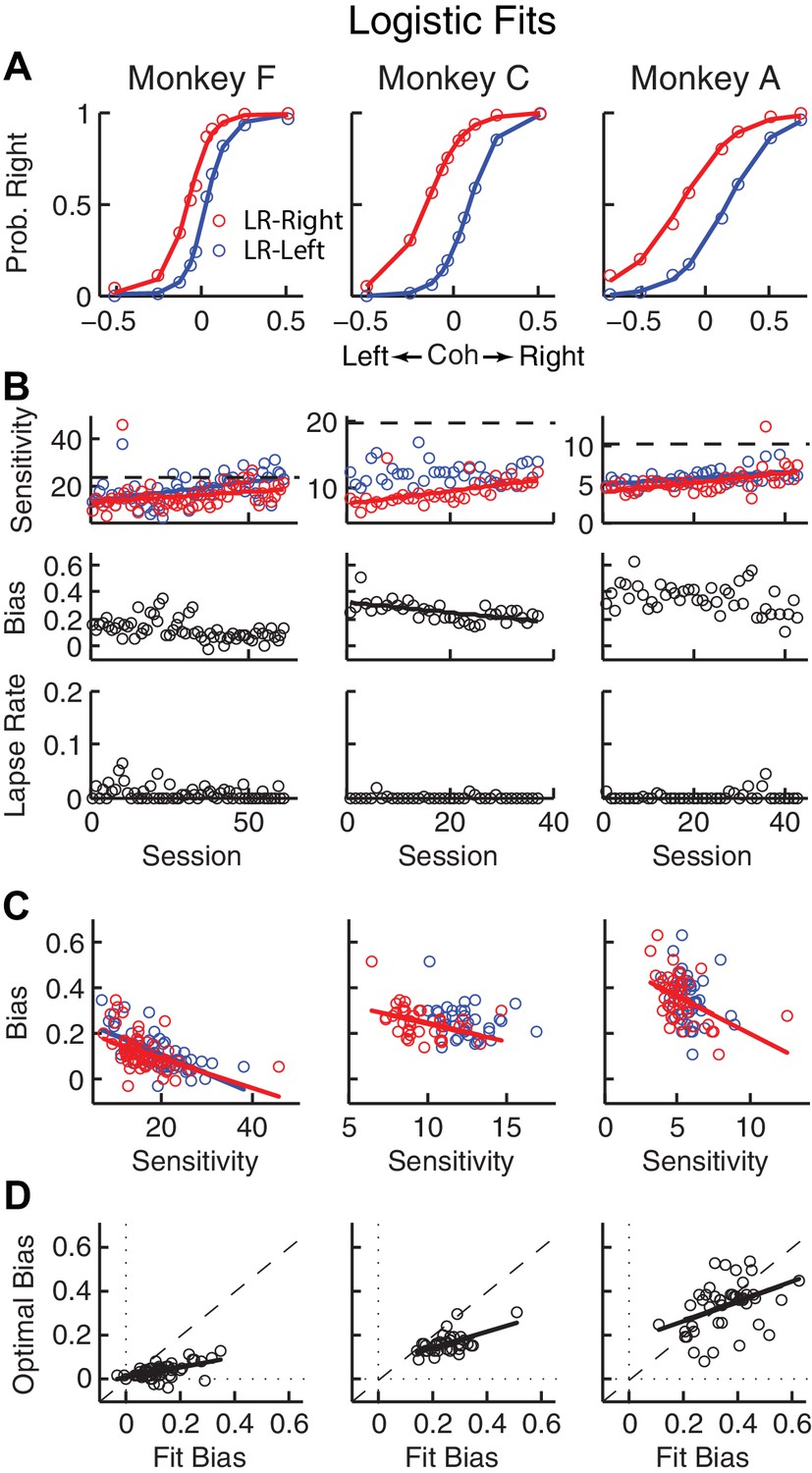
Relationships between sensitivity and bias from logistic fits to choice data.
(A) For each monkey, the probability of making a rightward choice is plotted as a function of signed coherence (–/+indicate left/right motion) from all sessions, separately for the two reward contexts, as indicated. Lines are logistic fits. (B) Top row: Motion sensitivity (steepness of the logistic function) in each context as a function of session index (colors as in A). Solid lines indicate significant positive partial Spearman correlation after accounting for changes in reward ratio across sessions (p<0.05). Black dashed lines indicate each monkey’s motion sensitivity for the task with equal rewards before training on this asymmetric reward task. Middle row: ΔBias (horizontal shift between the two psychometric functions for the two reward contexts at chance level) as a function of session index. Solid line indicates significant negative partial Spearman correlation after accounting for changes in reward ratio across sessions (p<0.05). Bottom row: Lapse rate as a function of session index (median = 0 for all three monkeys). (C) ΔBias as a function of motion sensitivity for each reward context (colors as in A). Solid line indicates a significant negative partial Spearman correlation after accounting for changes in reward ratio across sessions (p<0.05). (D) Optimal versus fitted Δbias. Optimal Δbias was computed as the difference in the horizontal shift in the psychometric functions in each reward context that would have resulted in the maximum reward per trial, given each monkey’s fitted motion sensitivity and experienced values of reward ratio and coherences from each session (see Figure 2—figure supplement 1). Solid lines indicate significant positive Spearman correlations (p<0.01). Partial Spearman correlation after accounting for changes in reward ratio across sessions are also significant for moneys F and C (p<0.05).
-
Figure 2—source data 1
Task parameters and the monkeys’ performance for each trial and each session.
The same data are also used in Figure 2—figure supplement 1, Figure 3, Figure 3—figure supplement 2, Figure 4 and Figure 4—figure supplement 1
- https://doi.org/10.7554/eLife.36018.006
-
Figure 2—source data 2
Source data for Figure 2—figure supplement 1.
Log-likelihood of the logistic regressions with and without sequential choice bias terms.
- https://doi.org/10.7554/eLife.36018.007
Figure 2—figure supplement 1
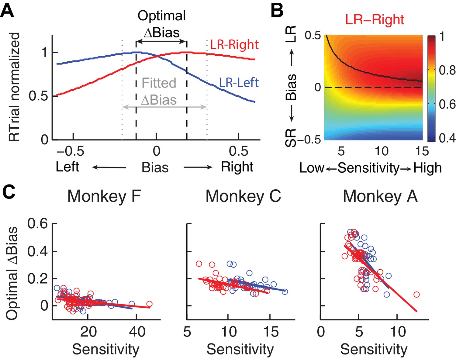
Relationship between bias and sensitivity.
(A), Identification of the optimal Δbias for an example session using logistic fits.
For each reward context (blue for LR-Left and red for LR-Right), RTrial was computed as a function of bias values sampled uniformly over a broad range, given the session-specific sensitivities, lapse rate, coherences, and large:small reward ratio. The optimal Δbias was defined as the difference between the bias values with the maximal RTrial for the two reward contexts. The fitted Δbias was defined as the difference between the fitted bias values for the two reward contexts. (B) The optimal bias decreases with increasing sensitivity. The example heatmap shows normalized RTrial as a function of sensitivity and bias values in the LR-Right blocks, assuming the same coherence levels as used for the monkeys and a large:small reward ratio of 2.3. The black curve indicates the optimal bias values for a given sensitivity value. (C) Scatterplots of optimal Δbiases obtained via the procedure described above as a function of sensitivity for each of the two reward contexts. Same format as Figure 2C Solid lines indicate significant partial Spearman correlation after accounting for changes in reward ratio across sessions (p<0.05). Note that the scatterplots of the monkeys’ Δbiases and sensitivities in Figure 2C also show negative correlations, similar to this pattern.
Figure 2—figure supplement 2
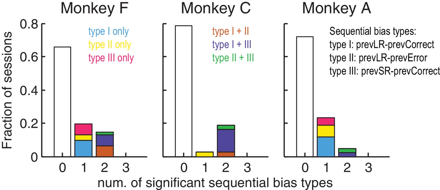
Monkeys showed minimal sequential choice biases.
Histogram of the fraction of sessions with 0, 1 or 2 types of sequential choice biases. Colors indicate the sequential bias types with respect to the previous reward (Large or Small) and outcome (Correct or Error), as indicated. Significant sequential bias effects were identified by a likelihood-ratio test for H0 : the sequential term in the logistic regression = 0, p<0.05.
Figure 3 with 2 supplements
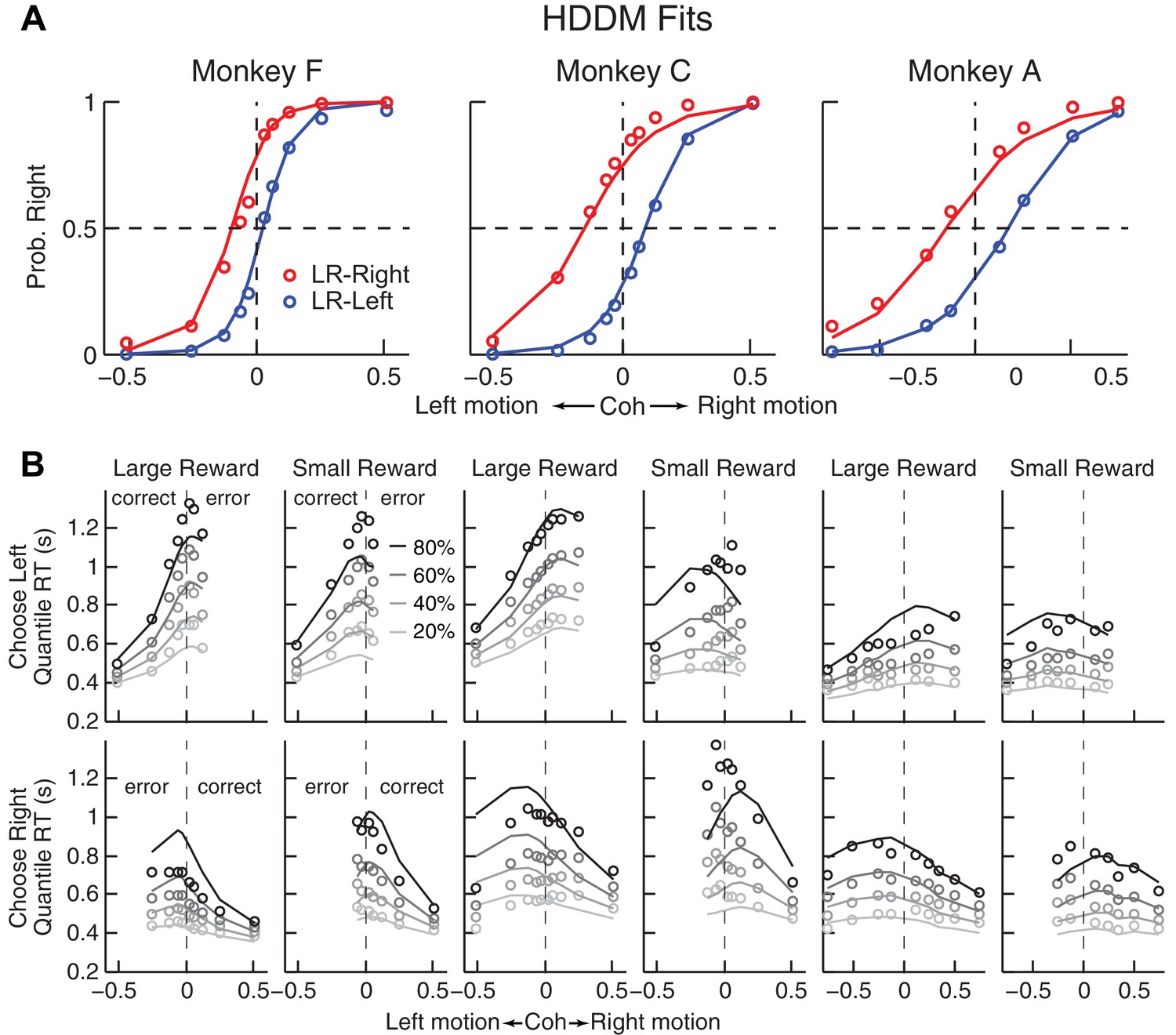
Comparison of choice and RT data to HDDM fits with both momentary-evidence (me) and decision-rule (z) biases.
(A) Psychometric data (points as in Figure 2A) shown with predictions based on HDDM fits to both choice and RT data. B, RT data (circles) and HDDM-predicted RT distributions (lines). Both sets of RT data were plotted as the session-averaged values corresponding to the 20th, 40 th, 60th, and 80th percentiles of the full distribution for the five most frequently used coherence levels (we only show data when > 40% of the total sessions contain >4 trials for that combination of motion direction, coherence, and reward context). Top row: Trials in which monkey chose the left target. Bottom row: Trials in which monkeys chose the right target. Columns correspond to each monkey (as in A), divided into choices in the large- (left column) or small- (right column) reward direction (correct/error choices are as indicated in the left-most columns; note that no reward was given on error trials). The HDDM-predicted RT distributions were generated with 50 runs of simulations, each run using the number of trials per condition (motion direction × coherence × reward context × session) matched to experimental data and using the best-fitting HDDM parameters for that monkey.
-
Figure 3—source data 1
Source data for Figure 3—figure supplement 2.
Collapsing-bound model fitting parameters and goodness of fits for each session.
- https://doi.org/10.7554/eLife.36018.011
Figure 3—figure supplement 1
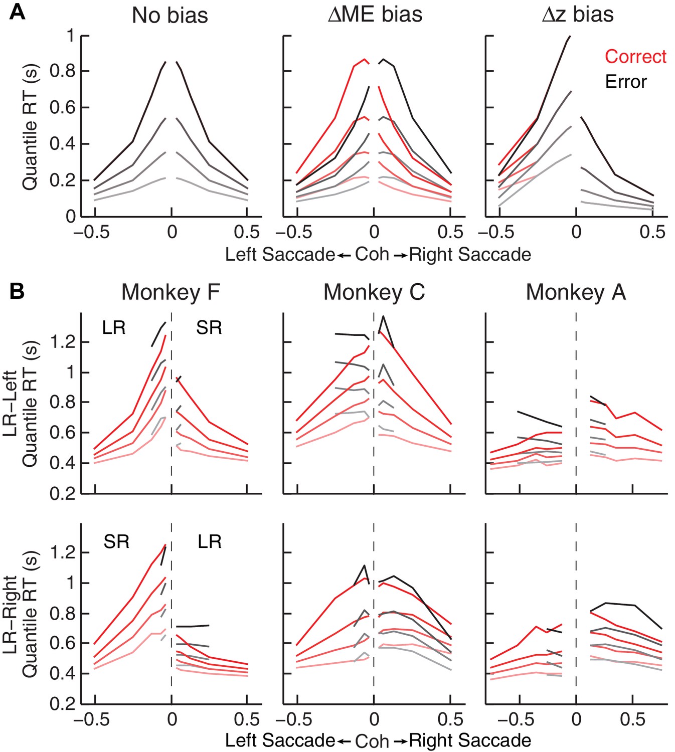
Qualitative comparison between the monkeys’ RT distribution and DDM predictions.
(A) RT distributions as predicted by a DDM with no bias in decision rule (z) or momentary evidence (me; left), with me > 0 (middle), and with z > 0.5 (right). RT distributions are shown separately for correct (red) and error (black) trials and using values corresponding to 20th, 40th, 60th, and 80th percentiles. The predictions assumed zero non-decision time to demonstrate effects on RT by only me or z biases. Positive/negative coh values indicate rightward/leftward saccades. The values of me and z were chosen to induce similar choice biases (~0.075 in coherence units). Note that the me bias induces large asymmetries in RT both between the two choices and between correct and error trials, whereas the z bias induces a large asymmetry in RT for the two choices, but with little asymmetry between correct and error trials. (B) The monkeys’ mean RTs for four quantiles for the LR-Right (top) and LR-Left (bottom) reward contexts, respectively (same convention as in A). Note the presence of substantial asymmetries between correct and error trials for all three monkeys.
Figure 3—figure supplement 2
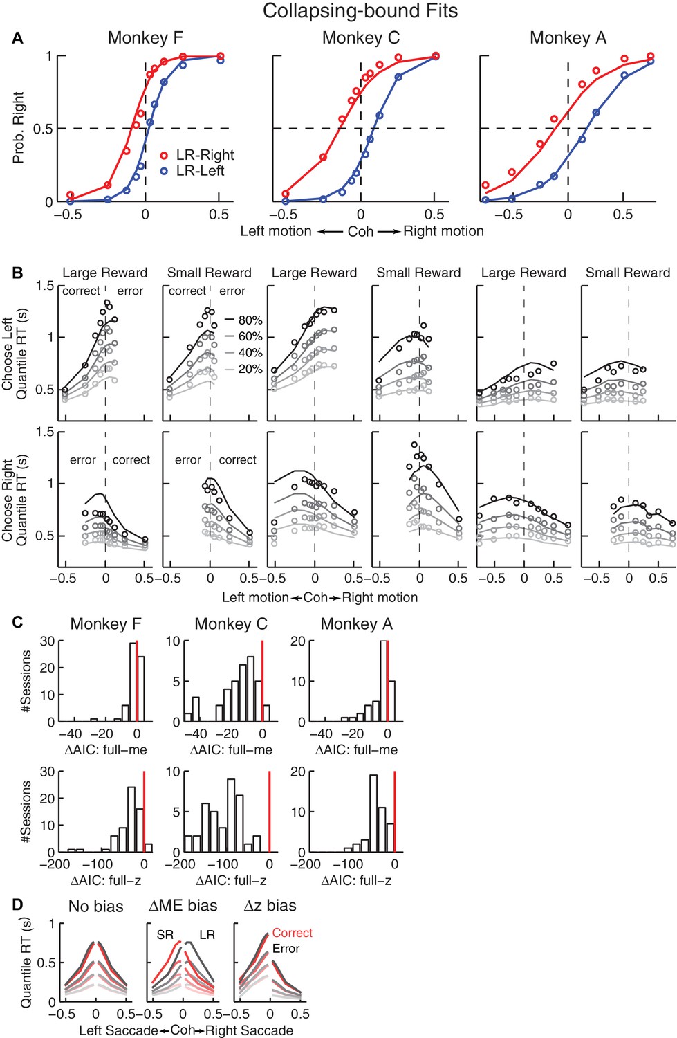
Fits to a DDM with collapsing bounds.
(A, B) A DDM with collapsing bounds and both momentary evidence (me) and decision rule (z) biases fit to each monkey’s RT data. Same format as Figure 3. (C) The model that included both me and z adjustments (‘full’) had smaller Akaike Information Criterion (AIC) values than reduced models (‘me’ or ‘z’ only) across sessions. Note also the different ranges of ΔAIC for the full–me and full–z comparisons. The mean ΔAIC (full-me) and ΔAIC (full-z) values are significantly different from zero (Wilcoxon signed rank test, p=0.0007 for Monkey F’s full–me comparison and p<0.0001 for all others). (D), RT distributions as predicted by the DDM with collapsing bounds, using no bias in z or me (left), me > 0 (middle), or z > 0.5 (right). Same format as Figure 3—figure supplement 1A.
Figure 4 with 2 supplements
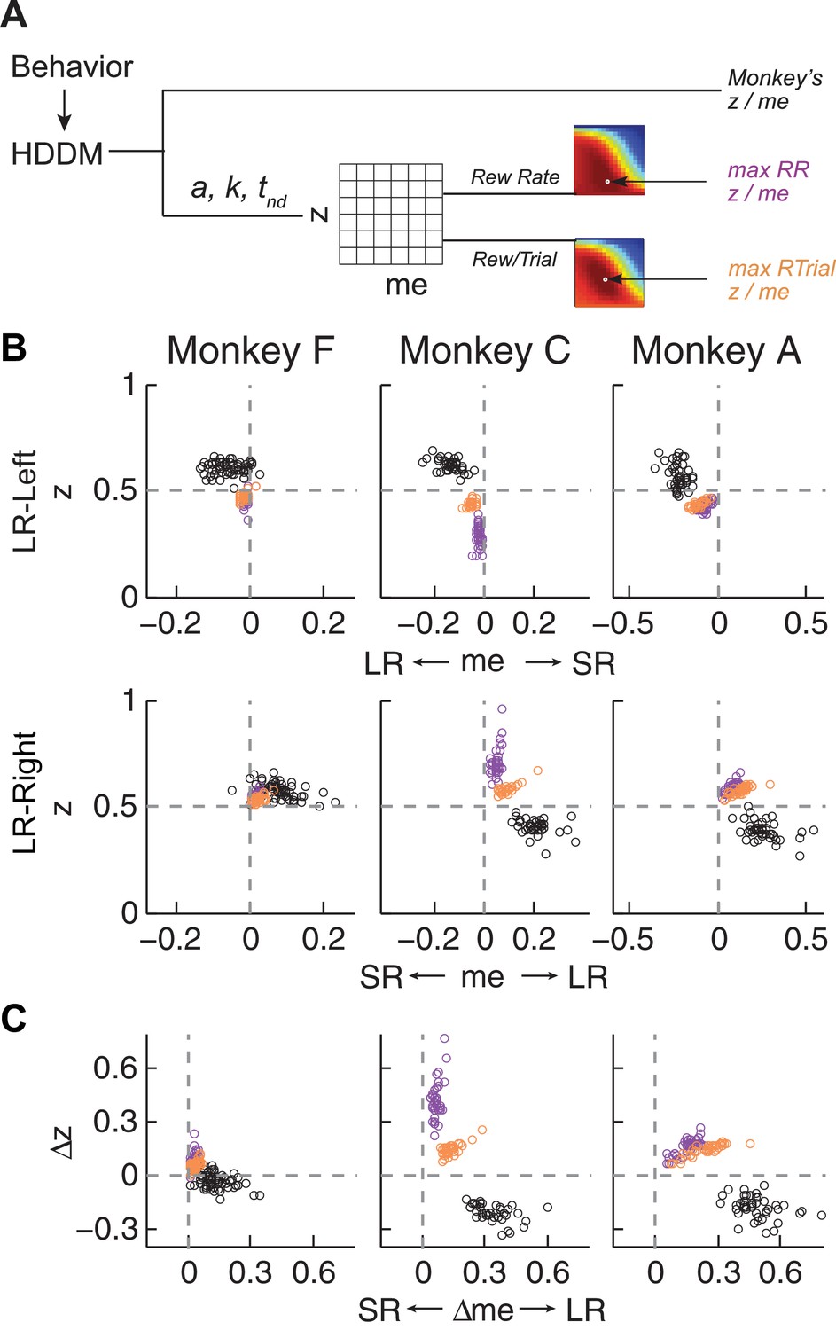
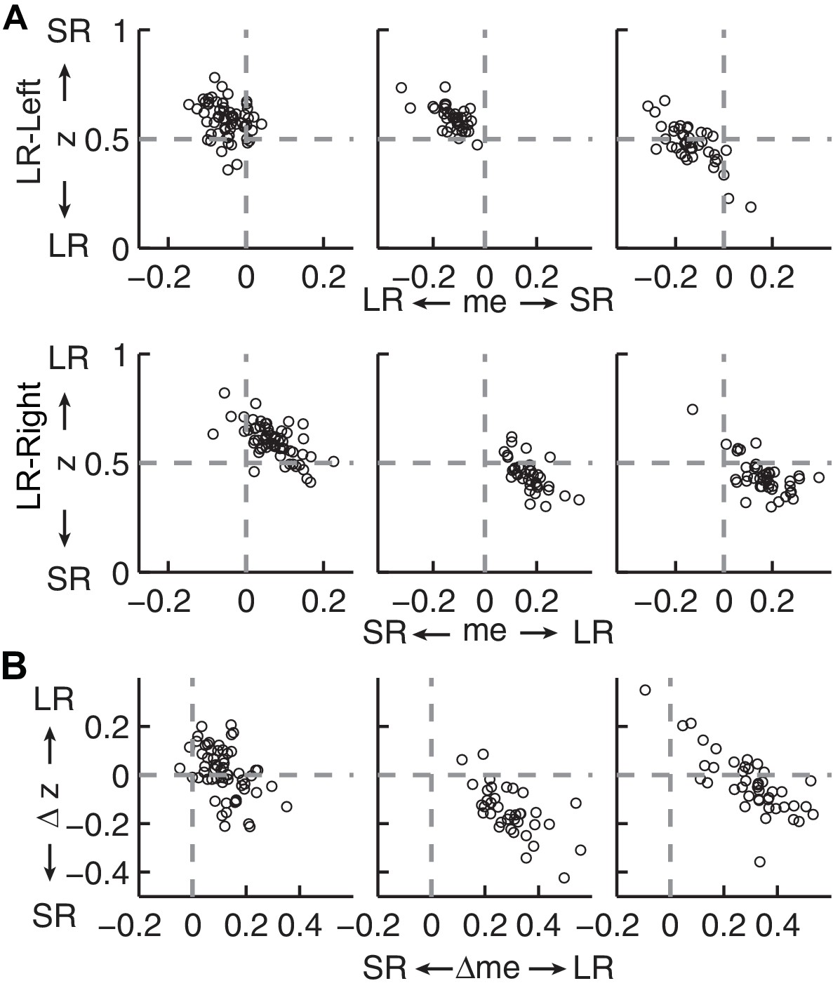
Actual versus optimal adjustments of momentary-evidence (me) and decision-rule (z) biases.
(A) Schematic of the comparison procedure. Choice and RT data from the two reward contexts in a given session were fitted separately using the HDDM. These context- and session-specific best-fitting me and z values are plotted as the monkey’s data (black circles in B and C). Optimal values were determined by fixing parameters a, k, and non-decision times at best-fitting values from the HDDM and searching in the me/z grid space for combinations of me and z that produced maximal reward function values. For each me and z combination, the predicted probability of left/right choice and RTs were used with the actual task information (inter-trial interval, error timeout, and reward sizes) to calculate the expected reward rate (RR) and average reward per trial (RTrial). Optimal me/z adjustments were then identified to maximize RR (purple) or RTrial (orange). (B) Scatterplots of the monkeys’ me/z adjustments (black), predicted optimal adjustments for maximal RR (purple), and predicted optimal adjustments for maximal RTrial (orange), for the two reward contexts in all sessions (each data point was from a single session). Values of me > 0 or z > 0.5 produce biases favoring rightward choices. (C) Scatterplots of the differences in me (abscissa) and z (ordinate) between the two reward contexts for monkeys (black), for maximizing RR (purple), and for maximizing RTrial (orange). Positive Δme and Δz values produce biases favoring large-reward choices.
-
Figure 4—source data 1
RTrial and RR function for each session and reward context.
The same data are used for Figure 5, Figure 5—figure supplement 1, Figure 6, Figure 6—figure supplement 1, Figure 7, Figure 7—figure supplement 1, Figure 8 and Figure 8—figure supplement 1
- https://doi.org/10.7554/eLife.36018.019
Figure 4—figure supplement 1
Estimates of momentary-evidence (me) and decision-rule (z) biases using the collapsing-bound DDM fits.
Same format as Figure 4B and C, except here only showing fits to the monkeys’ data. As with the model without collapsing bounds, the adjustments in me tended to favor the large reward but the adjustments in z tended to favor the small reward.
Figure 4—figure supplement 2
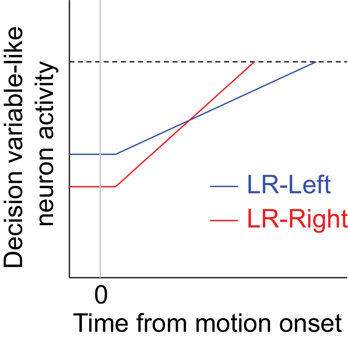
Hypothetical neural activity encoding a reward-biased perceptual decision variable.
The blue and red curves depict rise-to-threshold dynamics in favor of a particular (say, rightward) choice under the two reward contexts, as indicated. Note that when the rightward choice is paired with larger reward: 1) the slope of the ramping process, which corresponds to an adjustment in momentary evidence (me), is steeper; and 2) the baseline activity, which corresponds to the decision-rule (z) adjustment, is lower.
Figure 5 with 1 supplement
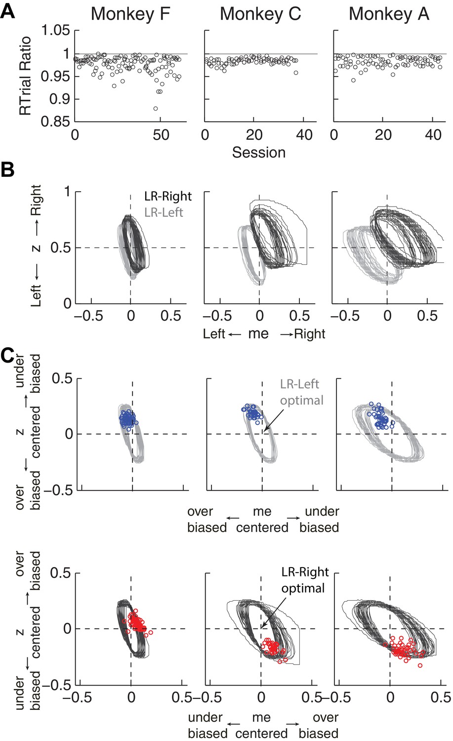
Predicted versus optimal reward per trial (RTrial).
(A) Scatterplots of RTrialpredict:RTrialmax ratio as a function of session index. Each session was represented by two ratios, one for each reward context. (B) 97% RTrialmax contours for all sessions, computed using the best-fitting HDDM parameters and experienced coherences and reward ratios from each session. Light grey: LR-Left blocks; Dark grey: LR-Right blocks. (C) The monkeys’ adjustments (blue: LR-Left blocks, red: LR-Right blocks) were largely within the 97% RTrialmax contours for all sessions and tended to cluster in the me over-biased, z under-biased quadrants (except Monkey F in the LR-Right blocks). The contours and monkeys’ adjustments are centered at the optimal adjustments for each session.
Figure 5—figure supplement 1
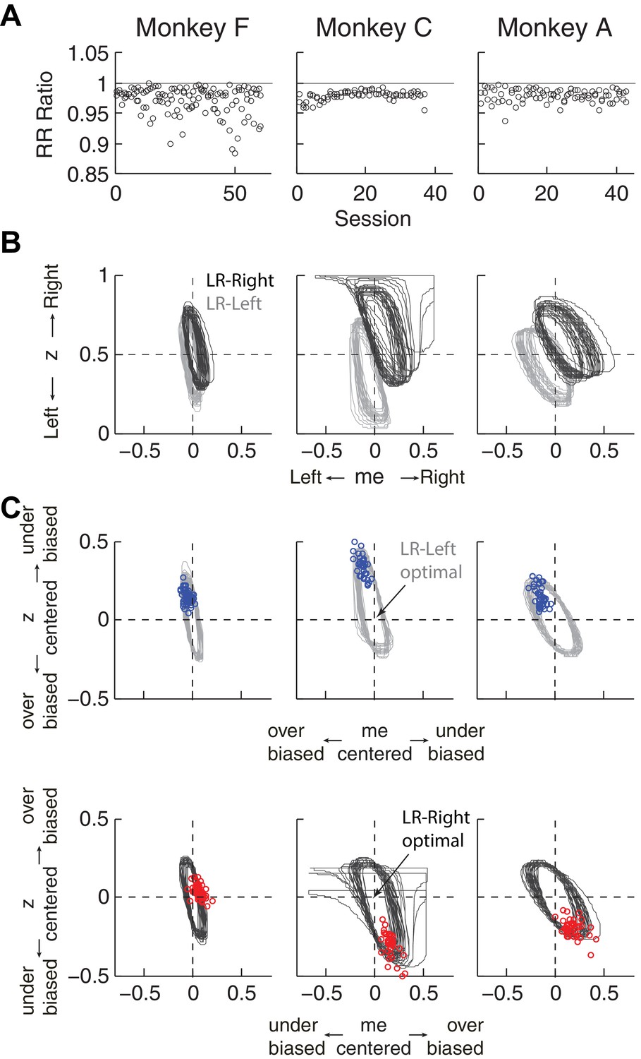
Predicted versus optimal reward rate (RR).
Same format as Figure 5. Mean RRpredict:RRmax ratio across sessions = 0.971 for monkey F, 0.980 for monkey C, and 0.980 for monkey A.
Figure 6 with 3 supplements
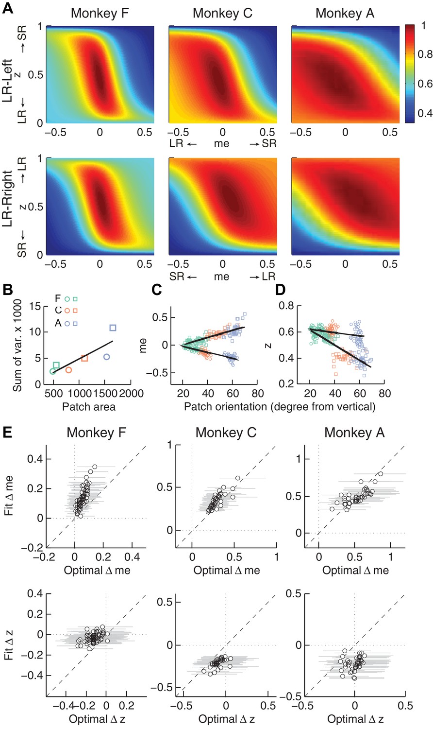
Relationships between adjustments of momentary-evidence (me) and decision-rule (z) biases and RTrial function properties.
(A) Mean RTrial as a function of me and z adjustments for the LR-Left (top) and LR-Right (bottom) blocks. Hotter colors represent larger RTrial values (see legend to the right). RTrial was normalized to RTrialmax for each session and then averaged across sessions. (B) Scatterplot of the total variance in me and z adjustments across sessions (ordinate) and the area of >97% max of the average RTrial patch (abscissa). Variance and patch areas were measured separately for the two reward blocks (circles for LR-Left blocks, squares for LR-Right blocks). (C, D) The monkeys’ session- and context-specific values of me (C) and z (D) co-varied with the orientation of the >97% heatmap patch (same as the contours in Figure 5B). Orientation is measured as the angle of the tilt from vertical. Circles: data from LR-Left block; squares: data from LR-Right block; lines: significant correlation between me (or z) and patch orientations across monkeys (p<0.05). Colors indicate different monkeys (see legend in B). E, Scatterplots of conditionally optimal versus fitted Δme (top row) and Δz (bottom row). For each reward context, the conditionally optimal me (z) value was identified given the monkey’s best-fitting z (me) values. The conditionally optimal Δme (Δz) was the difference between the two conditional optimal me (z) values for the two reward contexts. Grey lines indicate the range of conditional Δme (Δz) values corresponding to the 97% maximal RTrial given the monkeys’ fitted z (me) values.
Figure 6—figure supplement 1
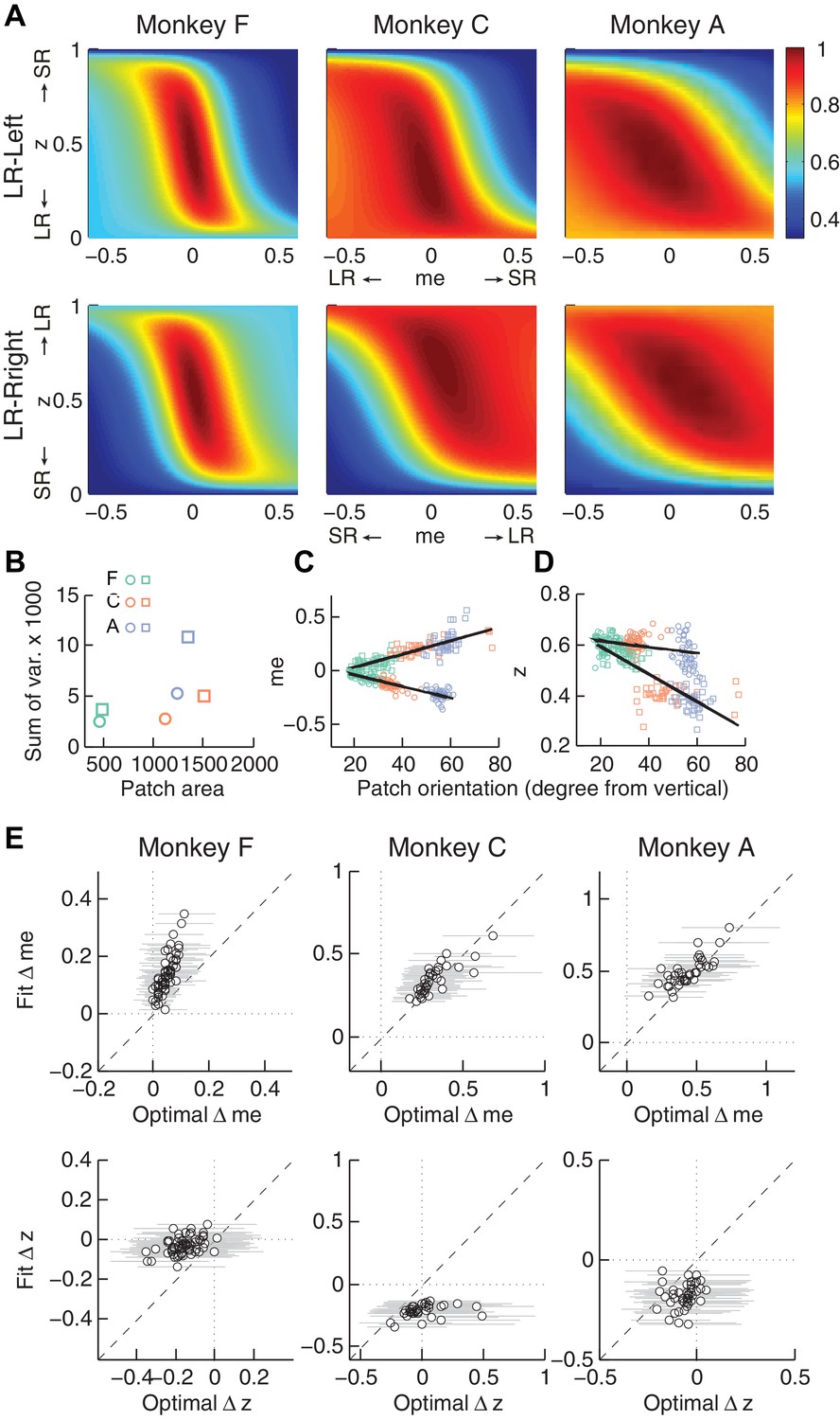
The monkeys’ momentary-evidence (me) and decision-rule (z) adjustments reflected RR function properties.
Same format as Figure 6, but using RR instead of RTrial.
Figure 6—figure supplement 2
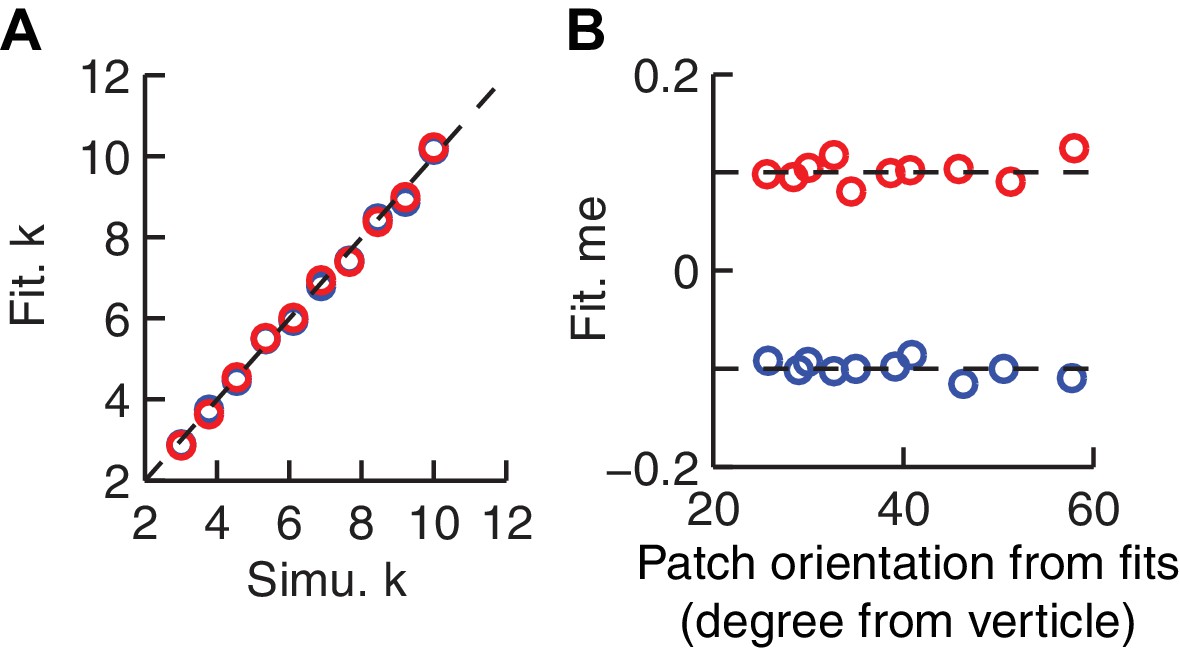
The HDDM model fitting procedure does not introduce spurious correlations between patch orientation and me value.
Artificial sessions were simulated with fixed me values (±0.1 for the two reward contexts) and different k values. (A) Recovered k values from HDDM fitting closely matched k values used for the simulations. (B) Recovered me values from HDDM fitting closely matched me values used for simulation and did not correlate with RTrial patch orientation.
Figure 6—figure supplement 3
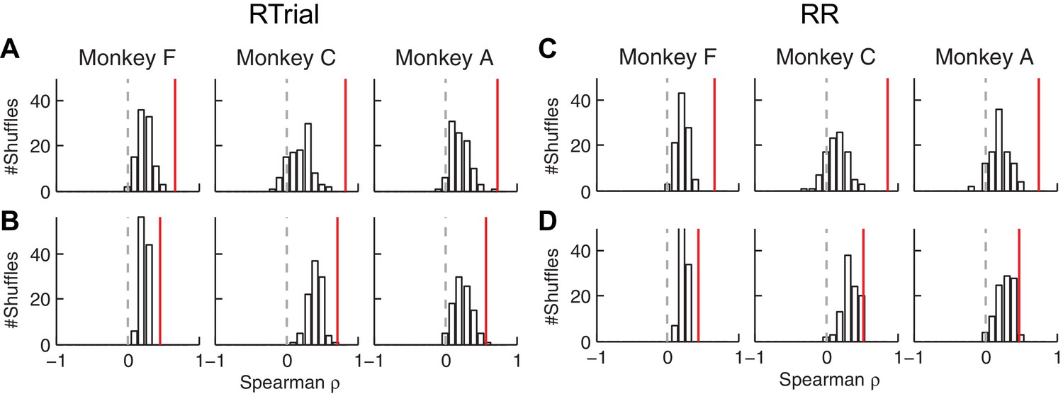
The correlation between fitted and conditionally optimal adjustments was stronger for the real, session-by-session data (red lines) than for unmatched (shuffled) sessions (bars).
(A, C) Momentary-evidence (Δme) adjustments. (B, D) Decision-rule (Δz) adjustments. (A, B) optimal values obtained with the RTrial function. (C, D) optimal values obtained with the RR function. Red lines indicate the partial Spearman correlation coefficients between the fitted and optimal Δme or Δz (obtained in the same way as the data in Figure 6E) for matched sessions. Bars represent the histograms of partial correlation for unmatched sessions, which were obtained by 100 random shuffles of the sessions (i.e., comparing the optimal and best-fitting values from different sessions). Note that the histograms for the unmatched sessions are centered at positive values, reflecting the non-session-specific tendency of reward surfaces to skew towards overly biased me and z values. The correlation values for matched sessions (red lines) are at even more positive values (Wilcoxson rank-sum test, p<0.001 for all three monkeys and both Δme and Δz), suggesting additional session-specific tuning of the me and z parameters.
Figure 7 with 1 supplement
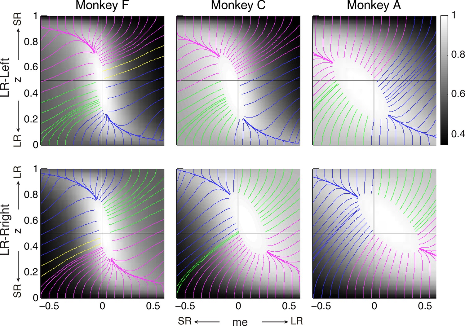
Relationships between starting and ending values of the satisficing, reward function gradient-based updating process.
Example gradient lines of the average RTrial maps for the three monkeys are color coded based on the end point of gradient-based me and z adjustments in the following ways: (1) me biases to large reward whereas z biases to small reward (magenta); (2) z biases to large reward whereas me biases to small reward (blue); (3) me and z both bias to large reward (green), and (4) me and z both bias to small reward (yellow). The gradient lines ended on the 97% RTrialmax contours. Top row: LR-Left block; bottom row: LR-Right block.
Figure 7—figure supplement 1
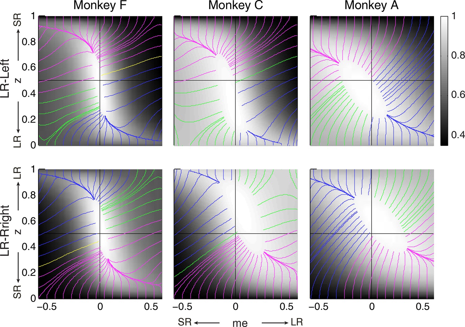
RR gradient trajectories color-coded by the end points of the me/z patterns.
Same format as Figure 7 but using gradients based on RR instead of RTrial.
Figure 8 with 4 supplements
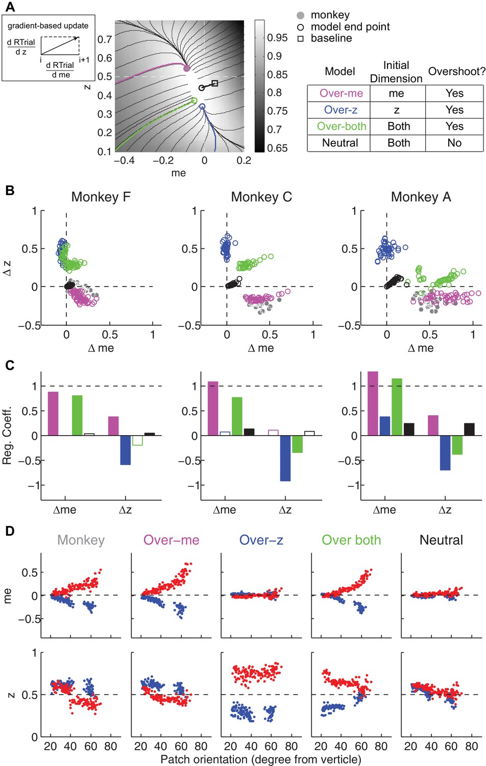
The satisficing reward function gradient-based model.
(A) Illustration of the procedure for predicting a monkey’s me and z values for a given RTrial function. For better visibility, RTrial for the LR-Left reward context in an example session is shown as a heatmap in greyscale. Gradient lines are shown as black lines. The square indicates the unbiased me and z combination (average values across the two reward contexts). The four trajectories represent gradient-based searches based on four alternative assumptions of initial values (see table on the right). All four searches stopped when the reward exceeded the average reward the monkey received in that session (RTrialpredict), estimated from the corresponding best-fitting model parameters and task conditions. Open circles indicate the end values. Grey filled circle indicates the monkey’s actual me and z. Note that the end points differ among the four assumptions, with the magenta circle being the closest to the monkey’s fitted me and z of that session. (B) Scatterplots of the predicted and actual Δme and Δz between reward contexts. Grey circles here are the same as the black circles in Figure 4C. Colors indicate model identity, as in (A). (C) Average regression coefficients between each monkey’s Δme (left four bars) and Δz (right four bars) values and predicted values for each of the four models. Filled bars: t-test, p<0.05. (D) Covariation of me (top) and z (bottom) with the orientation of the >97% maximal RTrial heatmap patch for monkeys and predictions of the four models. Blue: data from LR-Left blocks, red: data from LR-Right blocks. Data in the ‘Monkey’ column are the same as in Figure 6C and D. Note that predictions of the ‘over-me’ model best matched the monkey data than the other models.
Figure 8—figure supplement 1
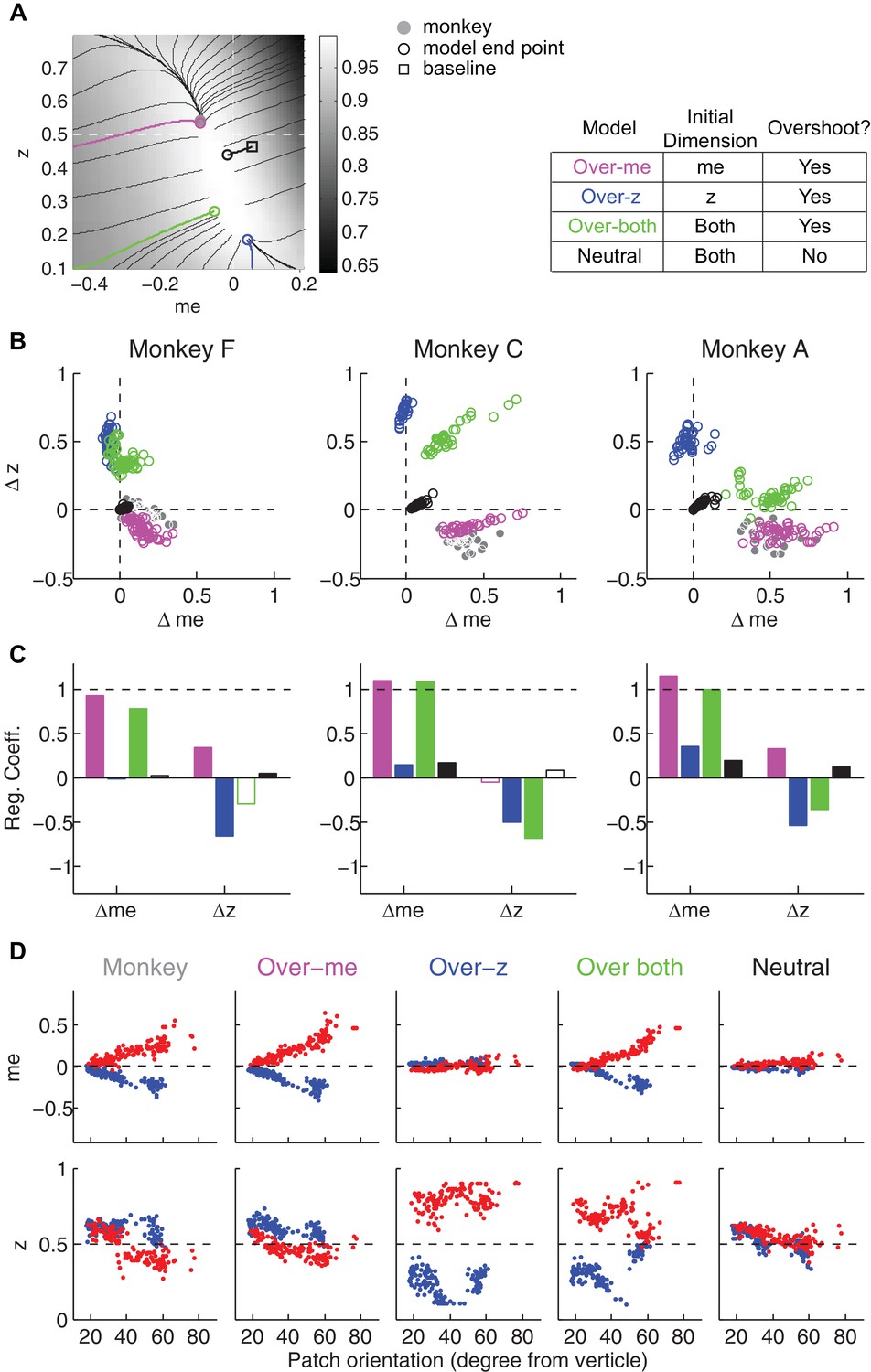
Predictions of a RR gradient-based model.
Same format as Figure 8 but using gradients based on RR instead of RTrial. The overly-biased starting me and z values were set as 90% of highest coherence level, and 0.1, respectively, except for the over-both model for one monkey C session (me = 88% * max(coh), z = 0.11) to avoid a local peak in the RR surface. Such local peaks at overly biased me and z values can divert the gradient-based updating process to even more biased values without ever reaching the monkey's final RR (e.g., the green trace at the bottom left corner in monkey C's LR-Left data in Figure 7—figure supplement 1).
Figure 8—figure supplement 2
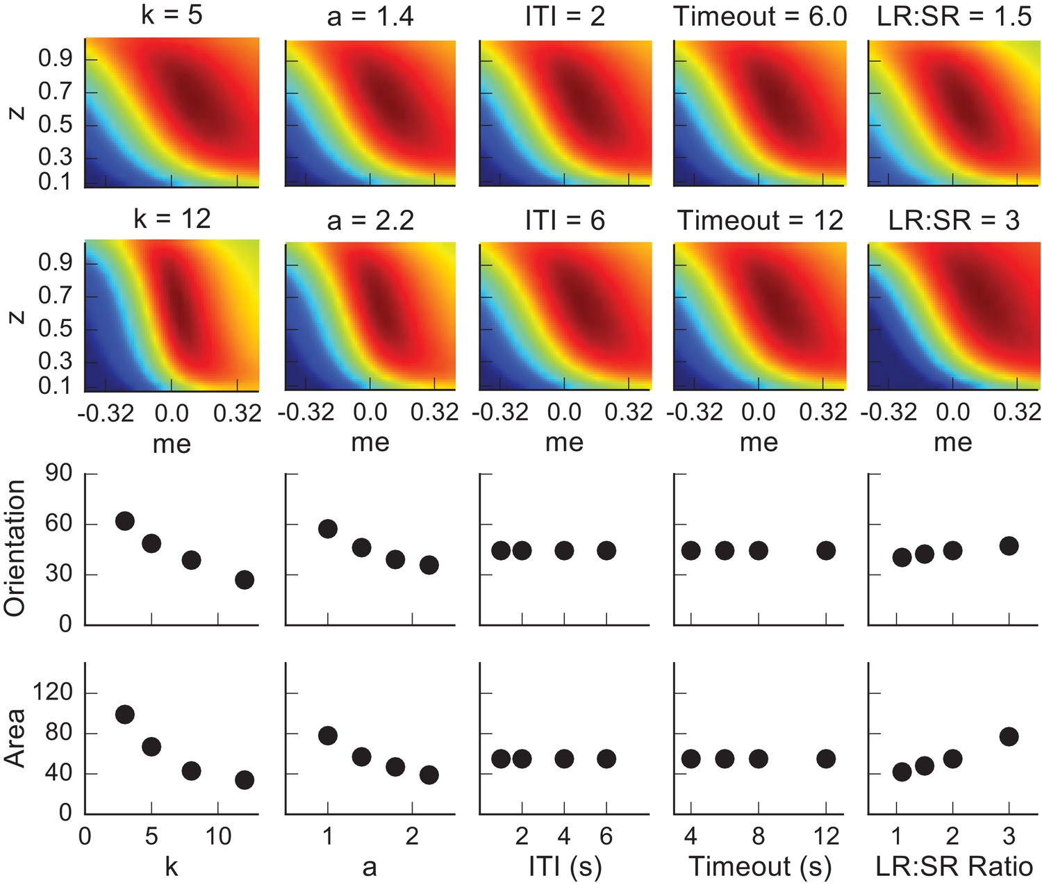
Dependence of the orientation and area of the near-optimal RTrial patch on parameters reflecting internal decision process and external task specifications.
The top two rows show the RTrial heatmaps with two values of a single parameter indicated above, while keeping the other parameters fixed at the baseline values. The third and fourth rows show the estimated orientation (the amount of tilt from vertical, in degrees) and area (in pixels), respectively, of the image patches corresponding to ≥97% of RTrialmax. The baseline values of the parameters are: a = 1.5, k = 6, non-decision times = 0.3 s for both choices, ITI = 4 s, Timeout = 8 s, large-reward (LR): small-reward (SR) ratio = 2.
Figure 8—figure supplement 3
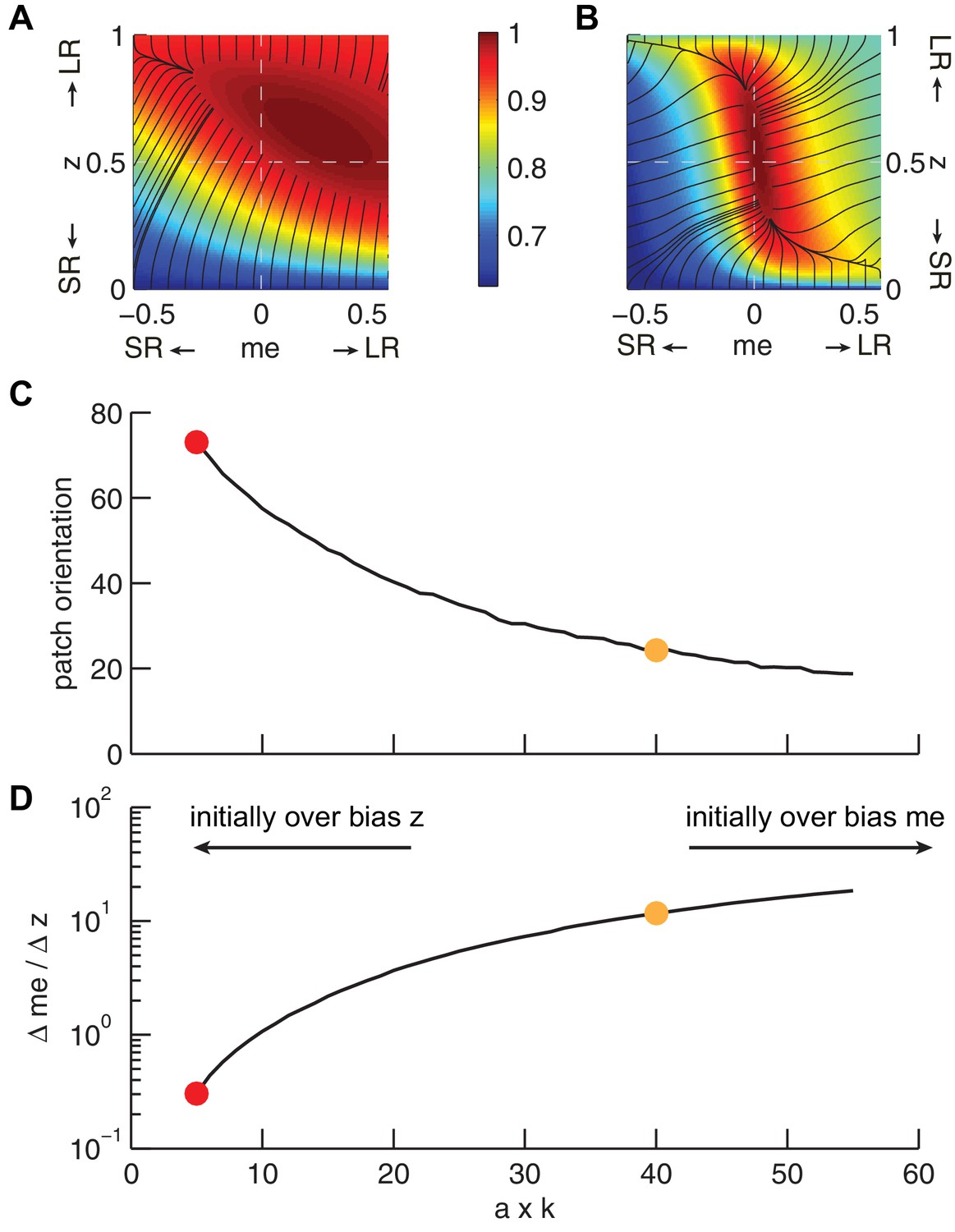
The joint effect of DDM model parameters a (governing the speed-accuracy trade-off) and k (governing perceptual sensitivity) on the shape of the reward function.
(A and B) Example RTrial functions corresponding to steeper gradients along the z (panel A, corresponding to the red points in panels C and D) or me (panel B, corresponding to the orange points in panels C and D) dimension. The gradient lines (black) stop when RTrial >0.97 of the maximum value. A: a = 1, k = 5. B: a = 1, k = 40. Large-reward:small-reward ratio = 2. (C), Orientation of the patch corresponding to >0.97 maximal RTrial as a function of the product of a and k. (D) The ratio of the mean gradients along the me and z dimensions as a function of the product of a and k. Our model assumes that the initial bias is along the dimension with the steeper gradient according to each monkey’s idiosyncratic RTrial function. Note that because me and z have different units, the boundary between initial-me and initial-z conditions may not correspond to a gradient ratio of 1.
Figure 8—figure supplement 4
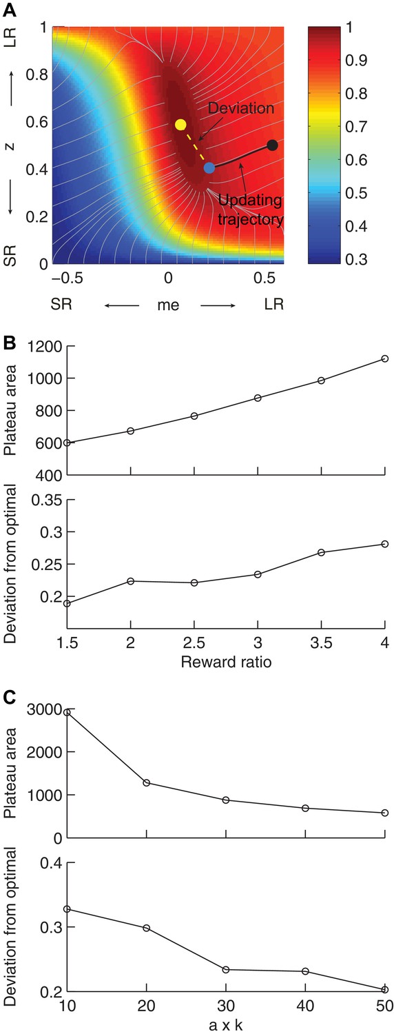
Effects of the shape of the reward function on deviations from optimality.
(A) Illustration of our heuristic updating model and measurement of deviation of the end point from optimal. Yellow dot: optimal solution. Gray lines: trajectory for gradient ascent, ending at 0.97 maximal RTrial. Black line: trajectory for updating from the starting point (black dot, me = 0.54, z = 0.5), which ended at 0.97 maximal RTrial (blue dot). The deviation of the end point from optimal is measured as the distance from the yellow dot to the blue dot (yellow dashed line). The same starting point and ending criterion were used for data shown in (B) and (C). (B) The area corresponding to >0.97 maximal RTrial plateau and end-point deviation from optimal increase with reward ratio. The product of a and k is fixed as 30. (C) The area corresponding to >0.97 maximal RTrial plateau and end-point deviation from optimal decrease with the product of a and k. Reward ratio is fixed as 3.
Author response image 1
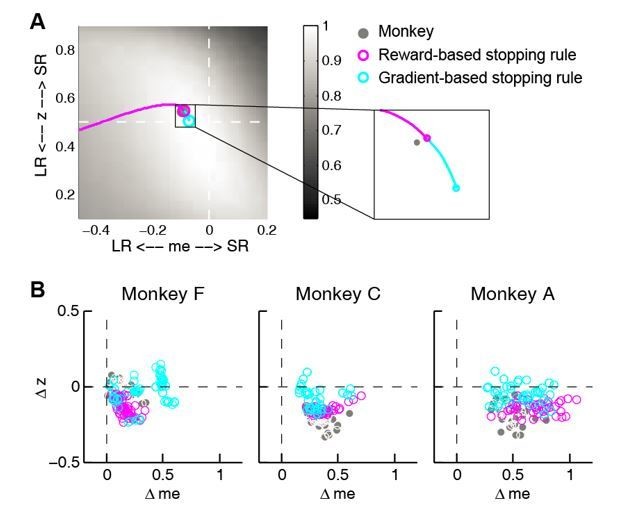
Comparison between reward and gradient-based updating process.
(A) example over-me reward (magenta) and gradient (cyan)-based updating process The same example as shown in Figure 8A. Gray circle indicates monkeys’ me and z. (B) Same format as Figure 8B. Scatterplot of end points for the two updating processes.
Author response image 2
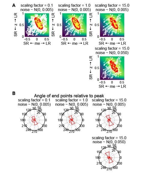
Gradient updating with randomness in the starting location and each updating step does not generate the biased end-point pattern seen in the data.
(A) Simulation of reward-gradient updating trajectories starting from random locations (white circles) on the reward function. Each updating step = scaling factor x gradient + noise (noise along the me and z dimensions were generated independently from the same Gaussian distribution). The updating process stopped when reward exceeded 97% of the maximum (red circles indicate end points). Note that the end-points of the updating process were located all around the reward-function plateau. The reward function was from the LR-R blocks in an example session of monkey C. (B) Polar histograms of the angle of the end-points relative to the peak of the reward function, showing end-points scattered all around the peak with clusters in two locations.
Tables
Table 1
Best-fitting parameters of HDDM.
https://doi.org/10.7554/eLife.36018.012| Monkey F (26079 trials) | Monkey C (37161 trials) | Monkey A (21089 trials) | ||||||||||
|---|---|---|---|---|---|---|---|---|---|---|---|---|
| LR-Left | LR-Right | LR-Left | LR-Right | LR-Left | LR-Right | |||||||
| Mean | Std | Mean | Std | Mean | Std | Mean | Std | Mean | Std | Mean | Std | |
| a | 1.67 | 0.16 | 1.43 | 0.12 | 1.77 | 0.09 | 1.53 | 0.13 | 1.33 | 0.13 | 1.36 | 0.09 |
| k | 10.22 | 1.87 | 9.91 | 2.11 | 6.58 | 0.51 | 5.08 | 0.92 | 4.04 | 0.33 | 3.45 | 0.46 |
| t1 | 0.31 | 0.03 | 0.29 | 0.03 | 0.35 | 0.04 | 0.33 | 0.05 | 0.29 | 0.04 | 0.27 | 0.04 |
| t0 | 0.28 | 0.04 | 0.31 | 0.05 | 0.33 | 0.04 | 0.31 | 0.03 | 0.21 | 0.08 | 0.26 | 0.04 |
| z | 0.60 | 0.03 | 0.57 | 0.04 | 0.62 | 0.03 | 0.40 | 0.04 | 0.57 | 0.06 | 0.39 | 0.04 |
| me | −0.06 | 0.04 | 0.08 | 0.05 | −0.14 | 0.04 | 0.21 | 0.06 | −0.22 | 0.05 | 0.27 | 0.09 |
-
Table 1—source data 1
HDDM model fitting parameters for each session.
The same data are also used in Figures 3, 4, 5, Figure 5—figure supplement 1, Figure 6, Figure 6—figure supplements 1, 2, 3, Figure 8 and Figure 8—figure supplement 1)
- https://doi.org/10.7554/eLife.36018.013
Table 2
The difference in deviance information criterion (ΔDIC) between the full model (i.e., the model that includes both me and z) and either reduced model (me-only or z-only), for experimental data and data simulated using each reduced model.
Negative/positive values favor the full/reduced model. Note that the ΔDIC values for the experimental data were all strongly negative, favoring the full model. In contrast, the ΔDIC values for the simulated data were all positive, implying that this procedure did not simply prefer the more complex model.
| Experimental data | Simu: me model | Simu: z model | ||||||
|---|---|---|---|---|---|---|---|---|
| ∆DIC: full - me | ∆DIC: full - z | ∆DIC: full - me | ∆DIC: full - z | |||||
| Mean | Std | Mean | Std | Mean | Std | Mean | Std | |
| Monkey F | −124.6 | 2.3 | −2560.4 | 5.2 | 3.1 | 9.8 | 0.2 | 11.8 |
| Monkey C | −1700.4 | 2.1 | −6937.9 | 1.3 | 17.5 | 11.3 | 1.8 | 1.3 |
| Monkey A | −793.6 | 3.4 | −2225.7 | 4.0 | 25.4 | 9.0 | 1.2 | 3.4 |
-
Table 2—source data 1
DIC for model fitting to the monkeys’ data and to the simulated data.
- https://doi.org/10.7554/eLife.36018.015
Additional files
-
Transparent reporting form
- https://doi.org/10.7554/eLife.36018.033
Download links
A two-part list of links to download the article, or parts of the article, in various formats.
Downloads (link to download the article as PDF)
Open citations (links to open the citations from this article in various online reference manager services)
Cite this article (links to download the citations from this article in formats compatible with various reference manager tools)
Ongoing, rational calibration of reward-driven perceptual biases
eLife 7:e36018.
https://doi.org/10.7554/eLife.36018


