Stochastic processes constrain the within and between host evolution of influenza virus
- University of Michigan, United States
Figures
Figure 1 with 4 supplements
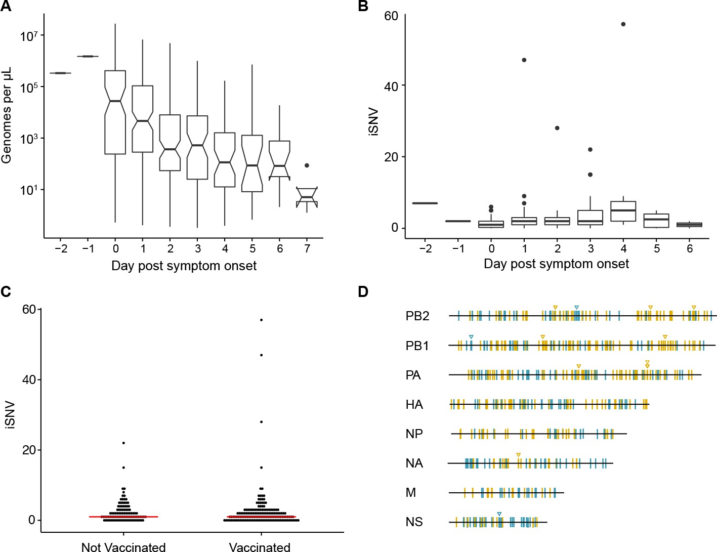
Within-host diversity of IAV populations.
(A) Boxplots (median, 25th and 75th percentiles, whiskers extend to most extreme point within median ±1.5 x IQR) of the number of viral genomes per microliter transport media stratified by day post symptom onset. Notches represent the approximate 95% confidence interval of the median. (B) Boxplots (median, 25th and 75th percentiles, whiskers extend to most extreme point within median ±1.5 x IQR) of the number of iSNV in 249 high quality samples stratified by day post symptom onset. (C) The number of iSNV in each isolate stratified by vaccination status. The red lines indicate the median. (D) Location of all identified iSNV in the influenza A genome. Mutations are colored nonsynonymous (blue) and synonymous (gold) relative to that sample’s consensus sequence. Mutations are considered nonsynonymous if they are nonsynonymous in any known influenza open reading frame. Triangles signify mutations that were found in more than one individual in a given season.
-
Figure 1—source data 1
Titers and day of sampling for all samples processed from the cohort.
- https://doi.org/10.7554/eLife.35962.008
-
Figure 1—source data 2
The number of iSNV and day of sampling for samples that qualified for iSNV identification.
- https://doi.org/10.7554/eLife.35962.009
-
Figure 1—source data 3
The number of iSNV and vaccination status for samples that qualified for iSNV identification.
- https://doi.org/10.7554/eLife.35962.010
-
Figure 1—source data 4
Location and frequency of iSNV identified in each individual.
(The highest quality sample was used when two where available).
- https://doi.org/10.7554/eLife.35962.011
Figure 1—figure supplement 1
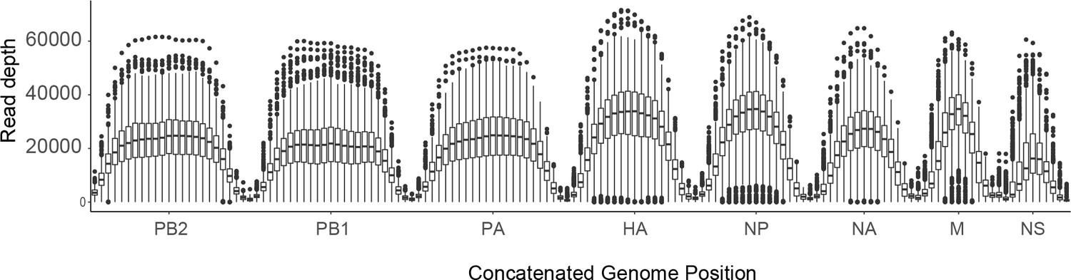
Sequence coverage for all samples.
For each sample, the sliding window mean coverage was calculated using a window size of 200 and a step of 100. The distributions of these means are plotted as box plots (median, 25th and 75th percentiles, whiskers extend to most extreme point within median ±1.5 x IQR) where the y-axis represents the read depth and the x-axis indicates the position of the window in a concatenated IAV genome.
Figure 1—figure supplement 2
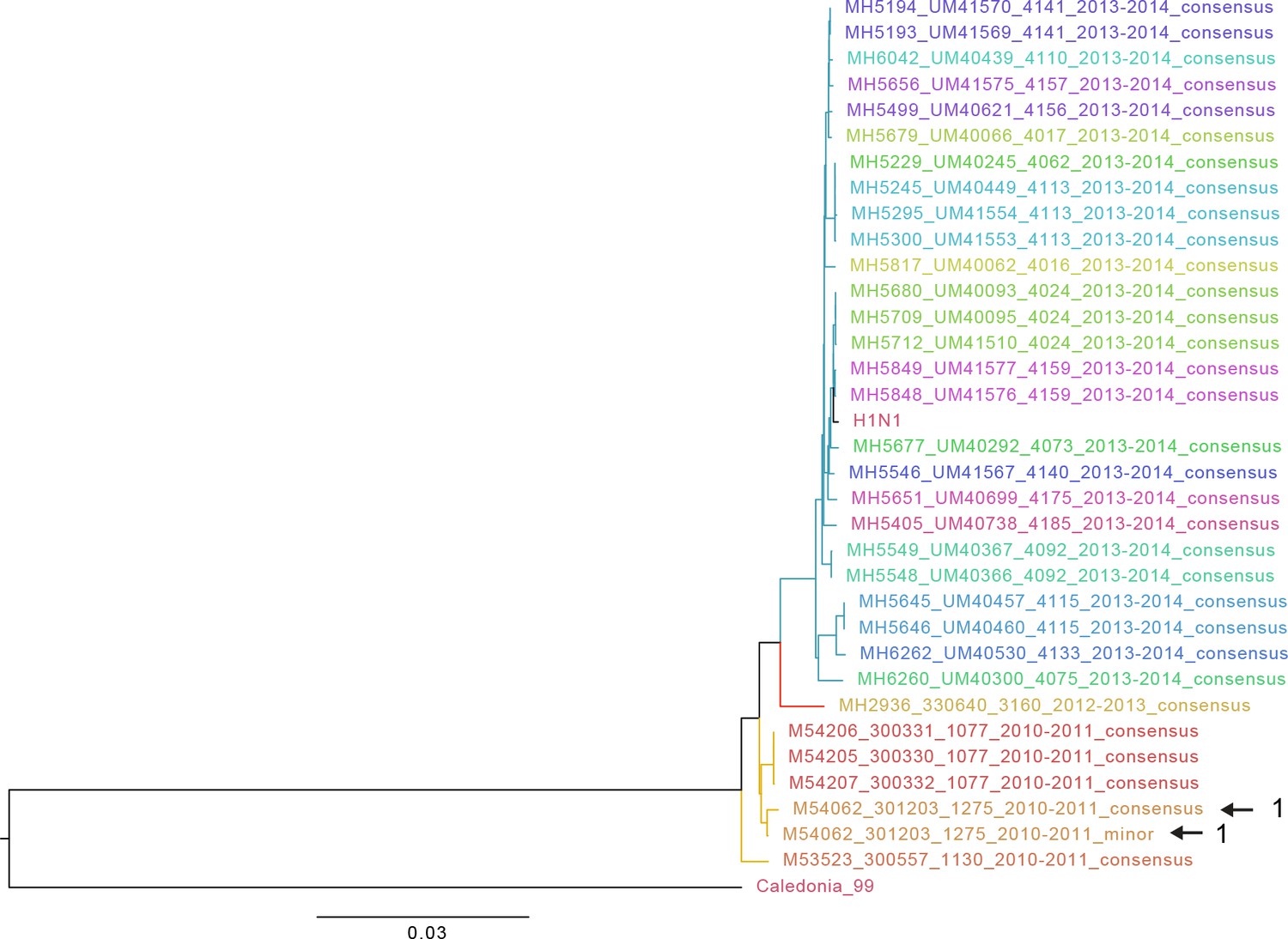
Approximate maximum likelihood trees of the concatenated coding sequences for high quality H1N1 samples.
The branches are colored by season; the tip identifiers are colored by household. Arrows with numbers indicate consensus and putative minor haplotypes for samples with greater than 10 iSNV. Trees were made using FastTree (Price et al., 2010). ‘Caledonia’ refers to A/New Caledonia/20/1999(H1N1). ‘H1N1’ refers to sequence from a plasmid clone derived from a clinical sample corresponding to A/California/07/2009.
Figure 1—figure supplement 3
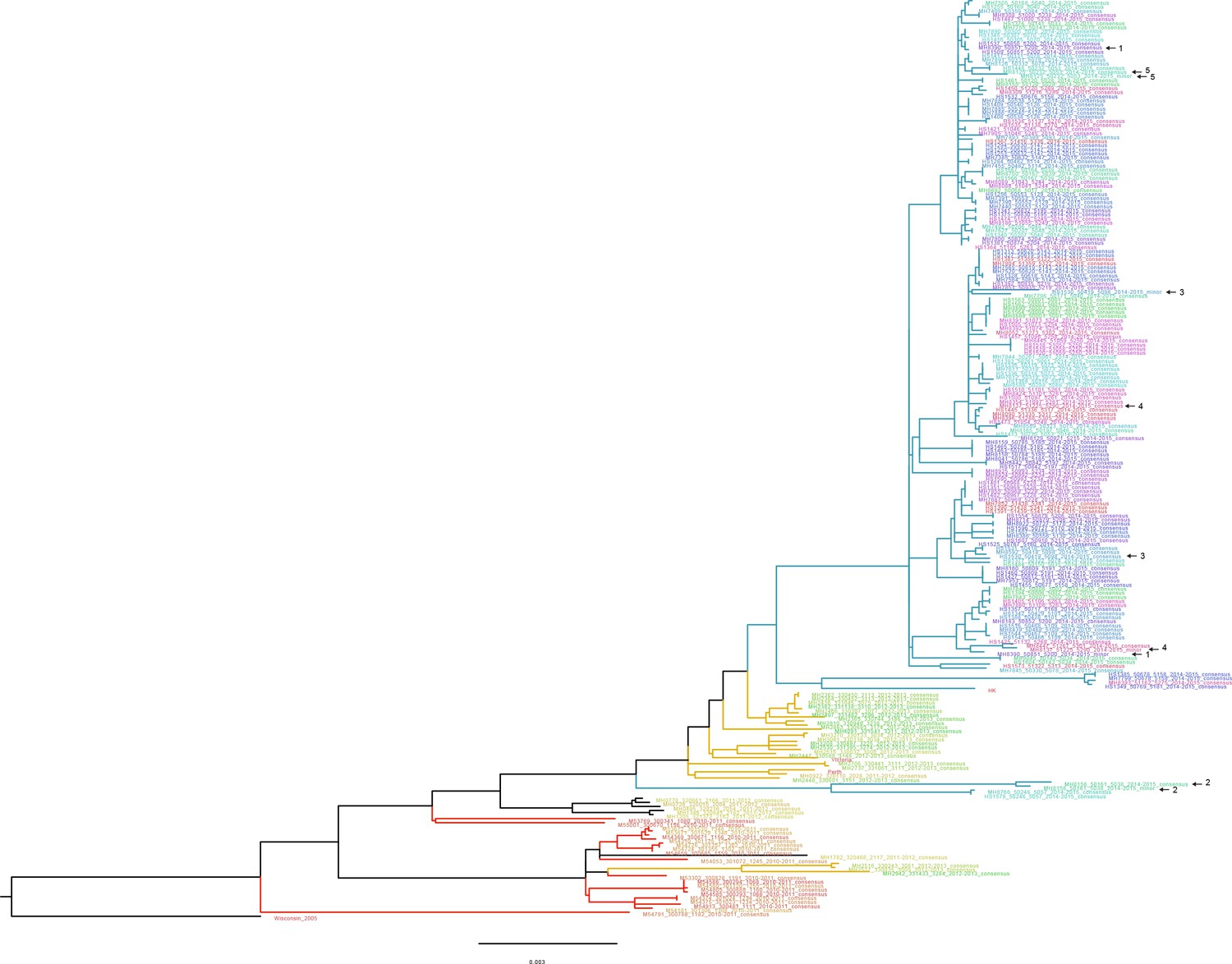
Approximate maximum likelihood trees of the concatenated coding sequences for high quality H3N2 samples.
The branches are colored by season; the tip identifiers are colored by household. Arrows with numbers indicate consensus and putative minor haplotypes for samples with greater than 10 iSNV. Trees were made using FastTree (Price et al., 2010). ‘Wisconsin_2005’ refers to A/Wisconsin/67/2005(H3N2). ‘Perth’, ‘Victoria’, and ‘HK’ refer to sequences from plasmid clones derived from clinical samples corresponding to A/Perth/16/2009, A/Victoria/361/2011, A/Hong Kong/4801/2014, respectively.
Figure 1—figure supplement 4
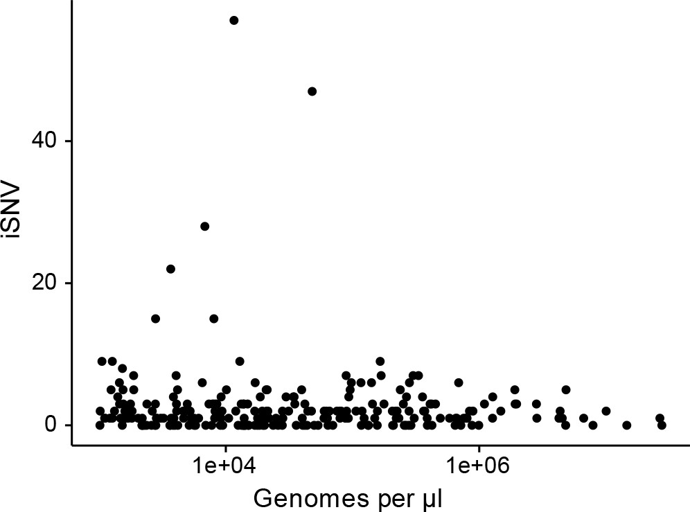
The effect of titer on the number of iSNV identified.
(A) The number of iSNV identified in an isolate (y-axis) plotted against the titer (x-axis, genomes/μl transport media).
Figure 2 with 1 supplement
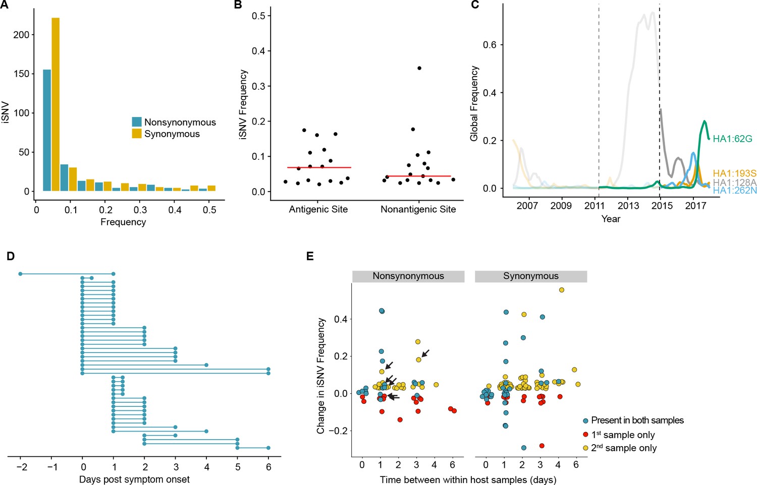
Within-host dynamics of IAV.
(A) Histogram of within-host iSNV frequency in 249 high quality samples. Bin width is 0.05 beginning at 0.02. As in Figure 1, mutations were classified as nonsynonymous (blue) if they were nonsynonymous in any known influenza reading frame. Synonymous mutations are gold. (B) The within-host frequency of nonsynonymous mutations in HA stratified by whether or not they are in known antigenic sites (p=0.46 Wilcoxon rank sum). (C) The global frequency of putative antigenic minority iSNV identified in our cohort that have circulated at frequencies above 5% globally since their time of collection. Each variant is labeled according the H3 numbering scheme. The dashed line indicates when samples were collected. Frequency traces are faded prior to the collection date. (D) Timing of sample collection for 43 paired longitudinal samples relative to day of symptom onset. Of the 49 total, 43 pairs had minority iSNV present in either sample. (E) The change in frequency over time for minority iSNV identified for the paired samples in (A). Nonsynonymous and synonymous iSNV are plotted separately. Mutations are colored according to whether they were detected in both isolates (blue), detected only the first isolate (red), or detected only in the second isolate (yellow). The threshold of detection was 2%. The arrows indicate mutations in known antigenic sites.
-
Figure 2—source data 1
The frequency and class (nonsynonymous/synonymous) of identified iSNV.
- https://doi.org/10.7554/eLife.35962.014
-
Figure 2—source data 2
Meta data for nonsynonymous iSNV found in HA.
- https://doi.org/10.7554/eLife.35962.015
-
Figure 2—source data 3
Frequency and meta data for antigenic iSNV that were also identified at the global level.
- https://doi.org/10.7554/eLife.35962.016
-
Figure 2—source data 4
Sampling day for within-host sample pairs.
- https://doi.org/10.7554/eLife.35962.017
-
Figure 2—source data 5
Frequencies of mutations identified in longitudinal sample pairs.
- https://doi.org/10.7554/eLife.35962.018
Figure 2—figure supplement 1
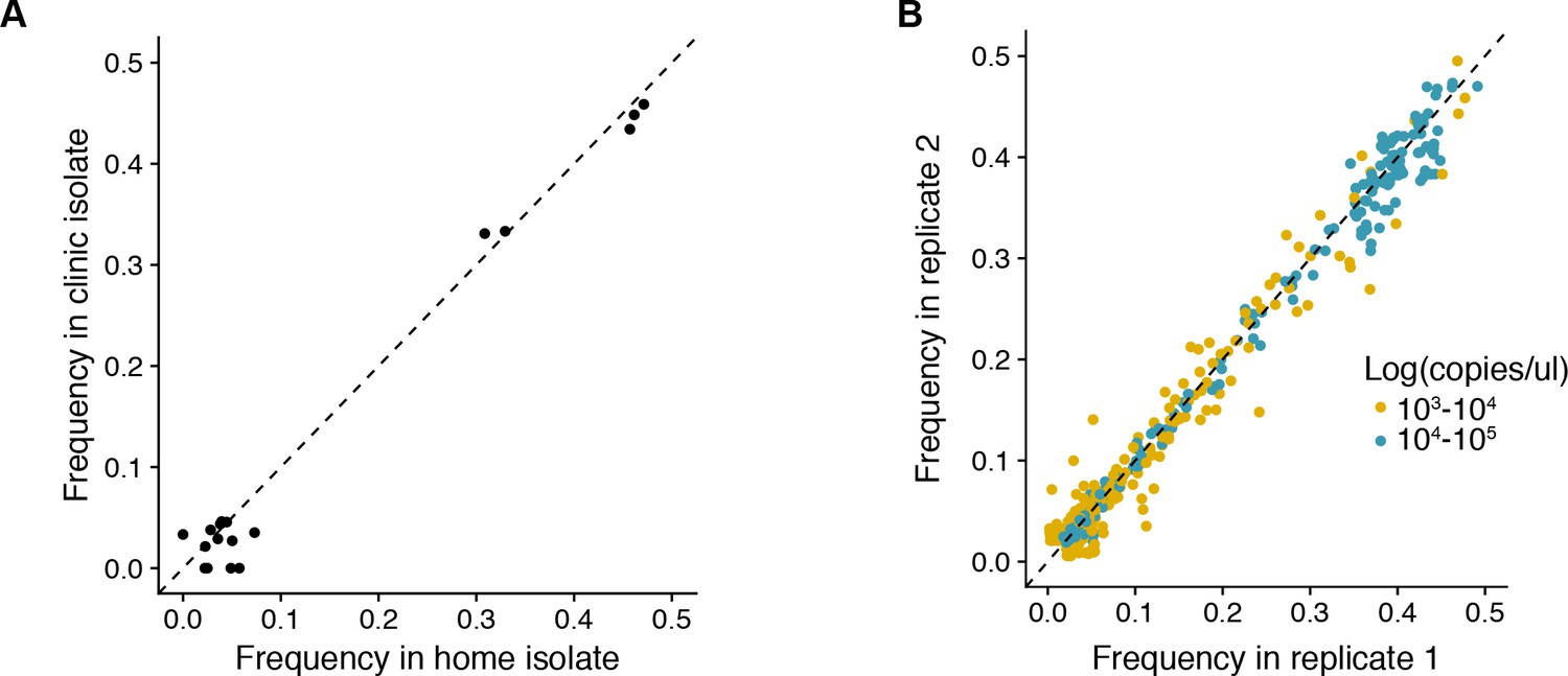
(A) Reproducibility of iSNV identification for paired samples acquired on the same day.
The x-axis represents iSNV frequencies found in the home-acquired nasal swab. The y-axis represents iSNV frequencies found the clinic-acquired combined throat and nasal swab. Dashed line is a one to one expectation. (B) Frequency of all minority iSNV as determined from replicate RT-PCR and sequencing libraries (see Materials and methods). Data are stratified by viral load of original samples. Note that samples with viral loads > 105 were not run in duplicate and those with viral loads < 103 were not used in the study. Dashed line is a one to one expectation.
Figure 3 with 1 supplement
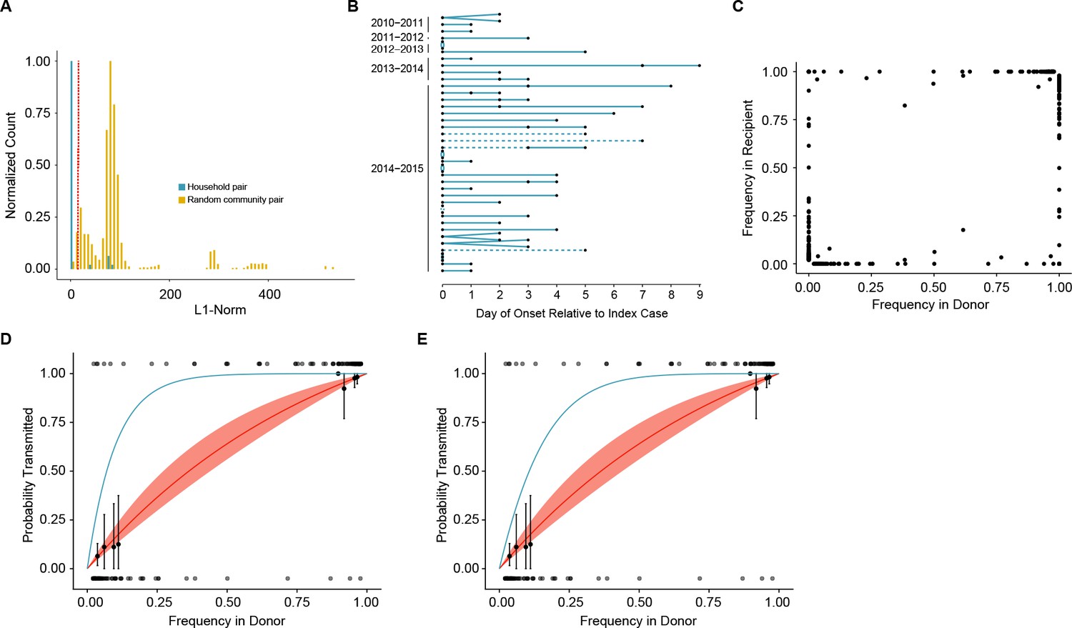
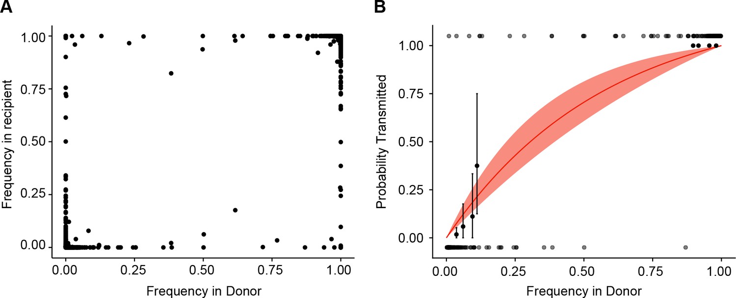
Between host dynamics of IAV.
(A) The distribution of pairwise L1-norm distances for household (blue) and randomly-assigned community (gold) pairs. The bar heights are normalized to the height of the highest bar for each given subset (47 for household, 1592 for community). The red line represents the 5th percentile of the community distribution. (B) Timing of symptom onset for 52 epidemiologically linked transmission pairs. Days of symptom onset for both donor and recipient individuals are indicated by black dots. Dashed lines represent pairs that were removed due to abnormally high genetic distance between isolates, see (A). (C) The frequency of donor iSNV in both donor and recipient samples. Frequencies below 2% and above 98% were set to 0% and 100% respectively. (D) The presence-absence model fit compared with the observed data. The x-axis represents the frequency of donor iSNV with transmitted iSNV plotted along the top and nontransmitted iSNV plotted along the bottom. The line represents the predicted probability of transmission given by the presence-absence model with a mean bottleneck of 1.68. The shaded regions represent the 95% confidence interval. Black points on the plot represent the probability of transmission estimated as the proportion of iSNV transmitted within a sliding window of width 5% and a step of 1%. The error bars represent the 95% confidence interval and were derived from a binomial distribution as in (Sobel Leonard et al., 2017). Only those windows with more than 5 iSNV are plotted. Blue curve shows the probability of transmission at a given frequency given a bottleneck size of 10 in the presence-absence model. (E) The beta-binomial model fit. Similar to (D), except the predicted outcomes are the based on a beta-binomial model using a mean bottleneck of 1.75. Blue curve shows the probability of transmission at a given frequency given a bottleneck size of 10 in the beta-binomial model.
-
Figure 3—source data 1
Genetic distance of household and community sample pairs.
- https://doi.org/10.7554/eLife.35962.021
-
Figure 3—source data 2
Day of onset and meta data for transmission pairs.
- https://doi.org/10.7554/eLife.35962.022
-
Figure 3—source data 3
Frequencies of iSNV identified in transmission pairs.
- https://doi.org/10.7554/eLife.35962.023
-
Figure 3—source data 4
The model prediction of the probability of transmission given donor frequency for the presence-absence model.
- https://doi.org/10.7554/eLife.35962.024
-
Figure 3—source data 5
The frequency of donor iSNV used in fitting transmission models.
- https://doi.org/10.7554/eLife.35962.025
-
Figure 3—source data 6
The model prediction of the probability of transmission given donor frequency for the beta-binomial model.
- https://doi.org/10.7554/eLife.35962.026
-
Figure 3—source data 7
Bottleneck estimates for all isolate pairings in cases where multiple donor or recipient isolates are available.
SPECID refers to specimen ID. Those beginning in M were taken at the clinic. Those beginning with HS were isolated at home.
- https://doi.org/10.7554/eLife.35962.027
Figure 3—figure supplement 1
Estimate of effective bottleneck size with relaxed variant calling criteria.
(A) The frequency of iSNV in both recipient and donor isolates. iSNV were identified using the original variant calling pipeline as in (McCrone and Lauring, 2016). (B) The presence-absence model fit as in Figure 3D with relaxed variant calling.
Tables
Table 1
Influenza viruses over five seasons in a household cohort
https://doi.org/10.7554/eLife.35962.002| 2010–2011 | 2011–2012 | 2012–2013 | 2013–2014 | 2014–2015 | |
|---|---|---|---|---|---|
| Households | 328 | 213 | 321 | 232 | 340 |
| Participants | 1441 | 943 | 1426 | 1049 | 1431 |
| Vaccinated, n (%)* | 934 (65) | 554 (59) | 942 (66) | 722 (69) | 992 (69) |
| IAV Positive Individuals† | 86 | 23 | 69 | 48 | 166 |
| H1N1 | 26 | 1 | 3 | 47 | 0 |
| H3N2 | 58 | 22 | 66 | 1 | 166 |
| IAV Positive Households‡ | |||||
| Two individuals | 13 | 2 | 9 | 7 | 23 |
| Three individuals | 5 | 2 | 3 | 3 | 11 |
| Four individuals | - | - | 1 | 2 | 4 |
| High Quality NGS Pairs§ | 4 | 1 | 2 | 6 | 39 |
-
*Self reported or confirmed receipt of vaccine prior to the specified season.
†RT-PCR confirmed infection.
-
‡Households in which two individuals were positive within 7 days of each other. In cases of trios and quartets, the putative chains could have no pair with onset > 7 days apart.
§Samples with > 103 genome copies per µl of transport medium, adequate amplification of all eight genomic segments, and average sequencing coverage > 103 per nucleotide.
Additional files
-
Supplementary file 1
Sensitivity and specificity of variant detection
- https://doi.org/10.7554/eLife.35962.028
-
Supplementary file 2
Nonsynonymous substitutions in HA antigenic sites
- https://doi.org/10.7554/eLife.35962.029
-
Supplementary file 3
Estimated bottleneck size for individual transmission pairs
- https://doi.org/10.7554/eLife.35962.030
-
Transparent reporting form
- https://doi.org/10.7554/eLife.35962.031
Download links
A two-part list of links to download the article, or parts of the article, in various formats.
Downloads (link to download the article as PDF)
Open citations (links to open the citations from this article in various online reference manager services)
Cite this article (links to download the citations from this article in formats compatible with various reference manager tools)
Stochastic processes constrain the within and between host evolution of influenza virus
eLife 7:e35962.
https://doi.org/10.7554/eLife.35962


