Bidirectional encoding of motion contrast in the mouse superior colliculus
- Northwestern University, United States
- Tianjin Medical University, China
- Tianjin Eye Hospital, China
- University of Virginia, United States
Figures
Figure 1 with 2 supplements
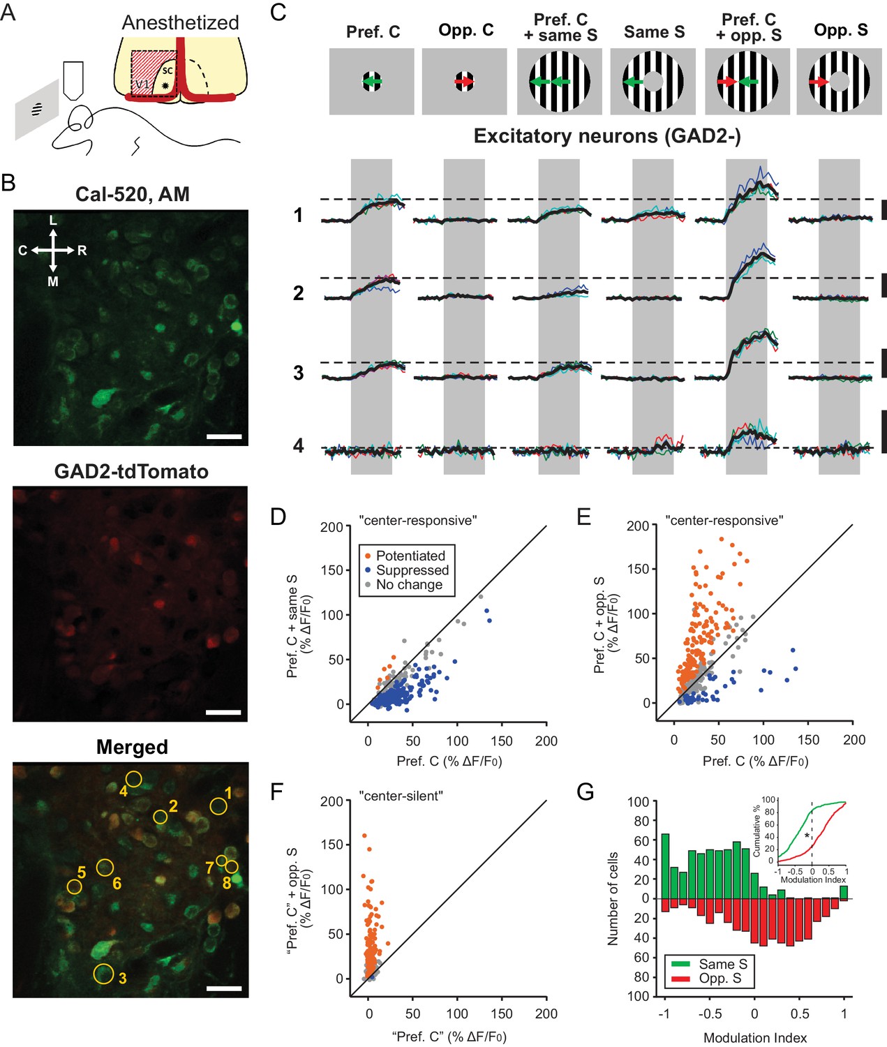
Excitatory neurons in the sSGS are bidirectionally modulated by motion direction in the receptive field surround.
(A) Two-photon calcium imaging in the mouse sSGS (bottom). Depiction of the surgical procedure to expose the SC, showing the removal of V1 (top). The star indicates a rough estimate of the imaging location. (B) Field of view containing sSGS neurons (at 20 μm below the surface) loaded with Cal-520 (top), GAD2+ neurons (expressing tdTomato) and GAD2- neurons (middle), and a merged image of both channels (bottom). Scale bars are 20 μm. R, rostral; C, caudal; M, medial; L, lateral. (C) Calcium signal of 4 GAD2- neurons in response to six chosen conditions of the center-surround (C-S) stimulus. C, center; S, surround; Pref, preferred; Opp, opposite. The diagrams on top are for illustration purpose only, while the actual preferred directions vary from cell to cell. The numbers on the left represent the neurons circled in (B, bottom). Neurons 5, 6, 7, and 8 are GAD2+, and their responses are shown in Figure 3A. Thin multicolored traces are individual trials, and thick black traces are the average. All scale bars represent 100% ΔF/F0. The dotted horizontal lines are aligned to the peak of the black trace in response to the preferred direction at the center. The gray boxes delimit the 2 s period of stimulus presentation. (D–E) Response comparison for individual center-responsive GAD2- neurons at the preferred center direction and when the preferred center was coupled with the same-direction surround (D), or when coupled with opposite-direction surround (E, n = 355 cells, 9 mice). (F) Same plot as (E), but for center-silent neurons. See Results and Materials and methods for the determination of the ‘preferred center direction’ for these neurons (n = 191 cells, 9 mice). (G) Modulation index distribution under same-surround (green) and opposite-surround (red) conditions (n = 355 + 191=546 cells, 9 mice). Both histograms and cumulative distributions (inset) are shown. The color scheme used in panels (D–F) illustrates the results of a bootstrapping test to determine the significance of the C-S modulation for individual neurons (orange indicates potentiation; blue, suppression; gray, no statistically significant change; See Materials and methods for details).
Figure 1—figure supplement 1
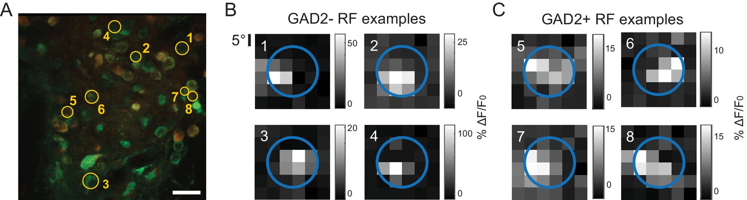
Example receptive fields of GAD2- and GAD2+ neurons in the sSGS.
(A) The same field of view depicted in Figure 1, with the same example neurons circled. (B,C) The mapped receptive fields (RFs) of those example GAD2- (B) and GAD2+ (C) neurons. Each RF is labeled by its corresponding neuron’s number. The blue circle represents the extent of spatial coverage by the center gratings stimulus.
Figure 1—figure supplement 2
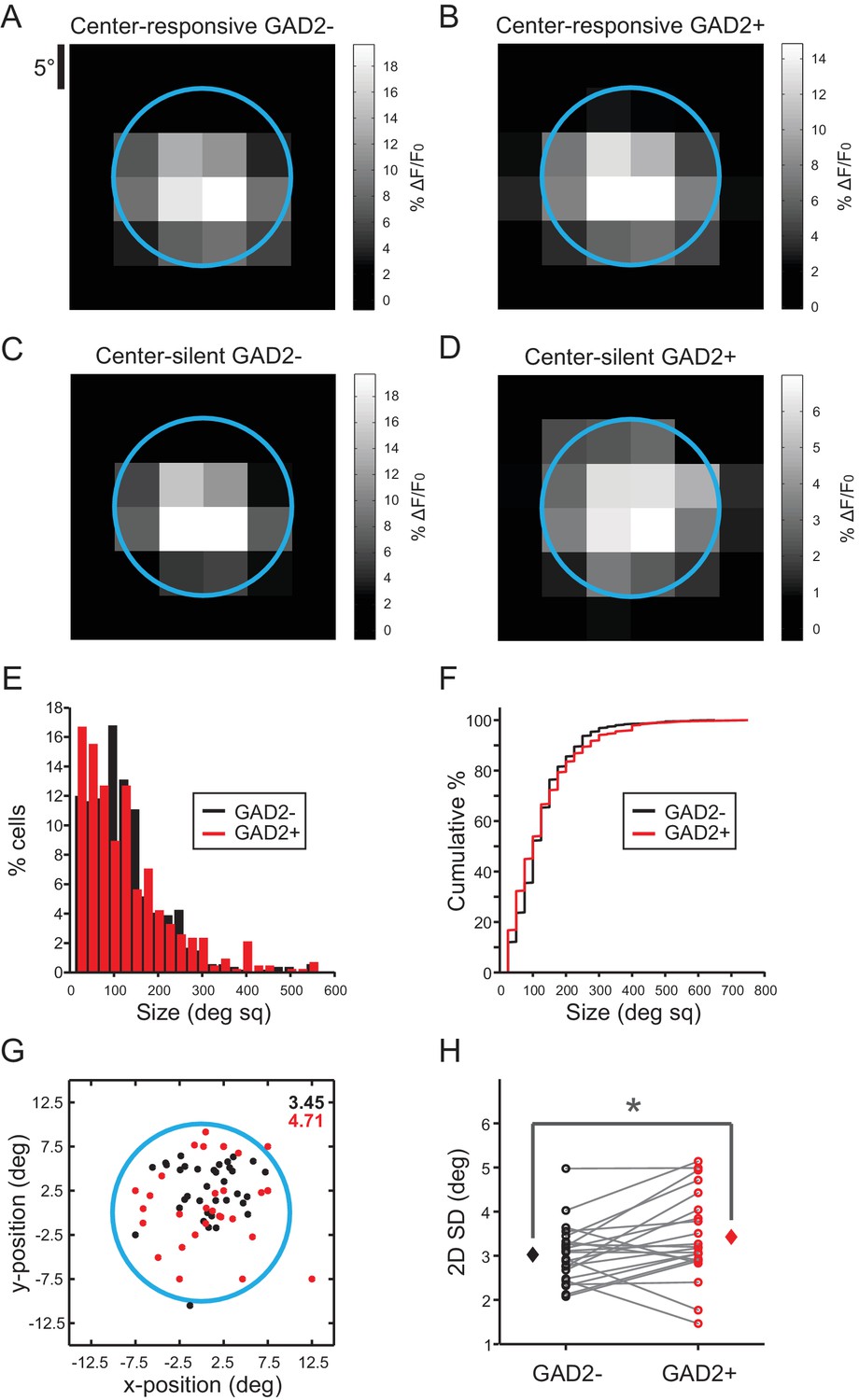
Receptive field properties of GAD2- and GAD2+ neurons in the sSGS.
(A) Average responses evoked by flashing black squares of GAD2- neurons that were responsive to the center drifting gratings stimulus (‘Center-responsive’, n = 355, 9 mice). The blue circle represents the extent of spatial coverage by the center gratings stimulus, which also applies to panels B-D. (B) Average responses of Center-responsive GAD2+ neurons (n = 379, 9 mice). (C) Average responses of GAD2- neurons that were silent to the separate presentations of center and surround but responded to a C-S combination (‘Center-silent’, n = 191, 9 mice). (D) Average responses of Center-silent GAD2+ neurons (n = 85, 9 mice). (E) Histogram of the receptive field size of GAD2- (black) and GAD2+ (red) cells that were responsive to the flashing square stimulus (n = 542 GAD2-; n = 425 GAD2+). (F) Cumulative distributions of the same data in (E) (p=0.19, Mann-Whitney U-test). (G) Receptive field centroids, mapped on the area where flashing squares were shown, of a population of GAD2- (black) and GAD2+ (red) neurons from a single imaging field of view. The corresponding values of the 2D standard deviation for each population is shown in the top right. The blue circle represents the extent of spatial coverage by the center gratings stimulus. (H) Comparison of the 2D standard deviations of GAD2- and GAD2+ neuronal populations from all imaged locations (n = 22 fields of view, 9 mice, p=0.03, paired t-test).
Figure 2 with 1 supplement
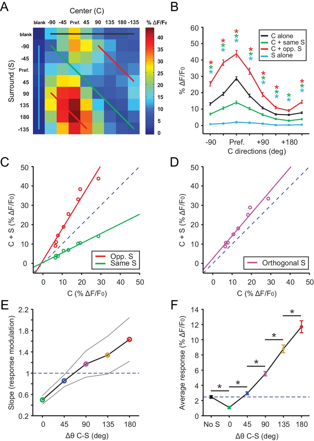
Excitatory neurons in the sSGS encode direction contrast.
(A) Averaged response matrix of center-responsive GAD2- neurons to all 81 combinations of the C-S stimulus, aligned to each cell’s preferred direction (n = 355 cells, 9 mice). The color scale to the right represents the response magnitude in % ΔF/F0. (B) Aligned and averaged population tuning curves for these neurons under particular C-S combinations. The x-axis represents the direction of the center stimulus relative to the preferred direction (‘Pref.”). The different colored curves represent the relationship of the surround to the center, corresponding to the same colored lines in (A). All data points are compared statistically to their corresponding points in the black tuning curve. (C) Geometric modulation of the center tuning curve by the two different surrounds in B; same surround induced divisive suppression (green, slope = 0.50, y-intercept = 0.48, R2 = 0.97), and opposite surround induced multiplicative potentiation (red, slope = 1.63, y-intercept = 1.55, R2 = 0.94). (D) Multiplicative potentiation of the center tuning curve by orthogonal-direction surrounds (slope = 1.17, y-intercept = 2.54, R2 = 0.96). The dashed blued lines in C and D are lines of identity. (E) The slopes of modulation illustrated in (C-D, corresponding colors) as well as the intermediate conditions vs. C-S direction difference (gray lines delimit the 95% confidence interval). The dashed blued line indicates a slope of 1, that is, no modulation. (F) Mean averaged responses (ΔF/F0) of center-silent GAD2- neurons vs. C-S direction difference (n = 191 cells, 9 mice). The dashed blue line is averaged ‘response’ to center alone. Data in B and F are presented as mean ± s.e.m. *: p<0.05, Mann-Whitney U-test.
Figure 2—figure supplement 1
Center-surround (‘C-S’) interactions in GAD2- neurons.
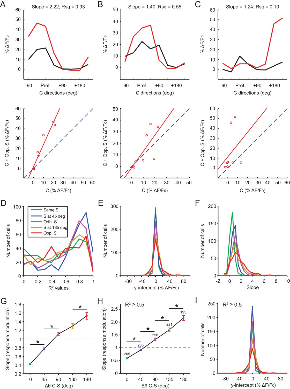
(A–C) Analysis of motion contrast encoding for individual center-responsive GAD2- cells (n = 355, 9 mice). Three examples are shown to illustrate the variability in goodness of fit. For each cell, its response to a particular C-S difference (red traces in top panels) was fitted to a first degree polynomial against its response to the corresponding center gratings alone (black traces in top panels). The fitted lines are shown in the bottom panels, and the slopes and R2 values are shown in the top panels. (D–F) Histograms of R2 values (D), y-intercept (E), and slopes (F), color coded by C-S combinations. (G) The fitted slope was averaged over all cells and plotted against the C-S difference (mean ± s.e.m, *: p<0.01, Mann-Whitney U-test). The dashed blue line is slope of 1, that is, no modulation. (H–I) Same plots as in (G) and (E), but only for fits where R2 ≥0.5 (mean ± s.e.m are shown in H, as well as the number of cells in each C-S category where R2 ≥0.5, *: p<0.01, Mann-Whitney U-test).
Figure 3 with 1 supplement
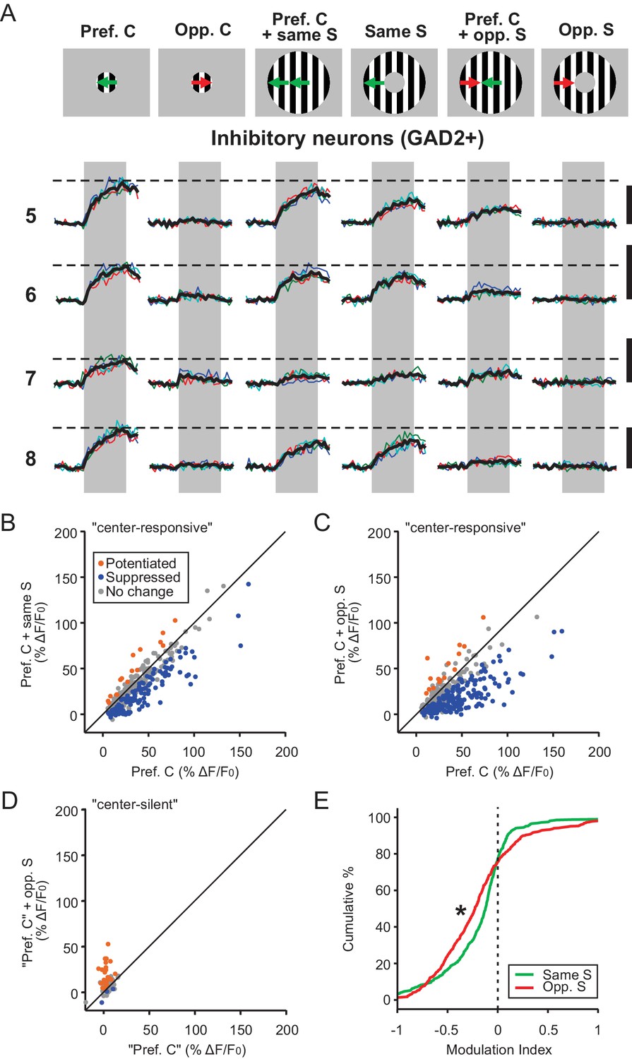
Inhibitory neurons in the sSGS are suppressed by direction contrast.
(A) Same as in Figure 1C, for four inhibitory neurons, with numbers on the left representing the neurons circled in Figure 1B, bottom. (B–C) Response comparison for individual center-responsive GAD2+ neurons to the preferred center direction and when the preferred center was coupled with same-direction surround (B), or opposite-direction surround (C, n = 379, 9 mice). The color scheme follows that in Figure 1D–F. (D) Response comparison for GAD2+ neurons that were silent to the separate presentations of center and surround but responded to a C-S combination, at the ‘preferred center’ and when coupled with the opposite-direction surround. See Materials and methods for the determination of the ‘preferred center’ for those neurons (n = 85 cells, 9 mice). (E) Modulation index distribution of neurons in (B–D) under same-surround (green) and opposite-surround (red) conditions (n = 379 + 85 = 464 cells, nine mice, KS test, p = 3.2e-6, KS stat = 0.17).
Figure 3—figure supplement 1
Center-surround interactions in GAD2+ neurons.
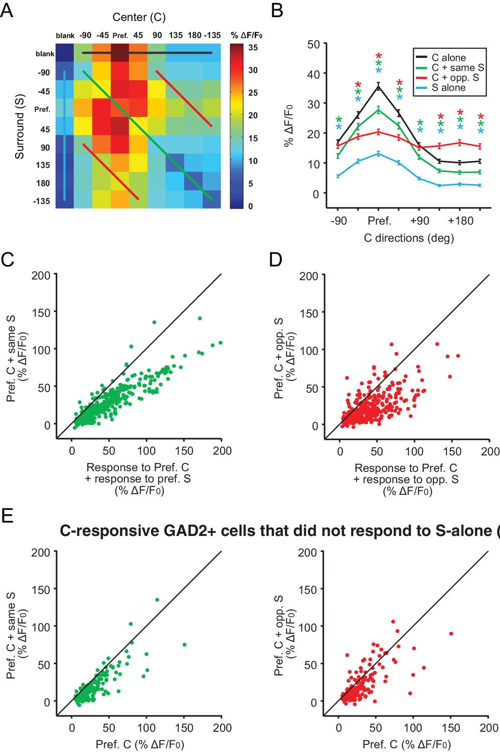
(A) Averaged response matrix of center-responsive GAD2+ neurons to all 81 combinations of the C-S stimulus, aligned to each cell’s preferred direction (n = 379 cells, 9 mice). The color scale to the right represents the response magnitude in % ΔF/F0. (B) Aligned and averaged population tuning curves for these neurons under particular C-S combinations. The x-axis represents the direction of the center stimulus relative to the preferred direction (Pref.). The different colored curves represent the relationship of the surround to the center, corresponding to the same colored lines in A. (C) Comparing these cells’ response to center +same surround against the sum of their responses to the Center and Surround stimuli alone. (D) Comparing these cells’ response to center + opposite surround against the sum of their responses to the Center and Surround stimuli alone. (E) Both same (left panel) and opposite surround (right) are still suppressive when only including cells that were not responsive to Surround stimulus alone.
Figure 4
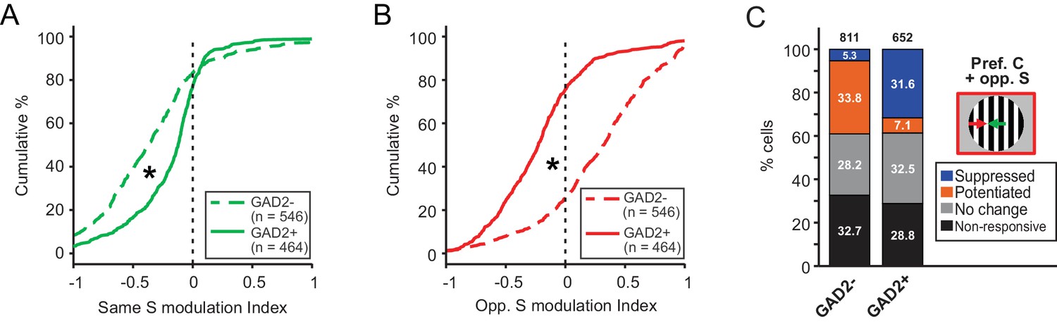
Excitatory and inhibitory sSGS neurons are differently modulated by the surround.
(A–B) Cumulative distributions of modulation index by same surround (A) or opposite surround (B) in GAD2- (dashed lines) and GAD2+ cells (solid lines). The distributions are the same as in Figure 1G and Figure 3E, grouped here to highlight the differences between the two cell types. (C) Percentages of GAD2- and GAD2+ neurons in four response categories (determined by a bootstrapping test) to the presentation of the preferred center + opposite surround combination: non-responsive, non-modulated, potentiated, and suppressed. Values in the boxes represent the percentage of neurons in each category; numbers at the top represent the total numbers of neurons in the study. The ‘non-responsive’ category included neurons that did not respond to any of the C-S conditions and a small population of neurons that responded to the surround alone, but not the center stimulus.
Figure 5
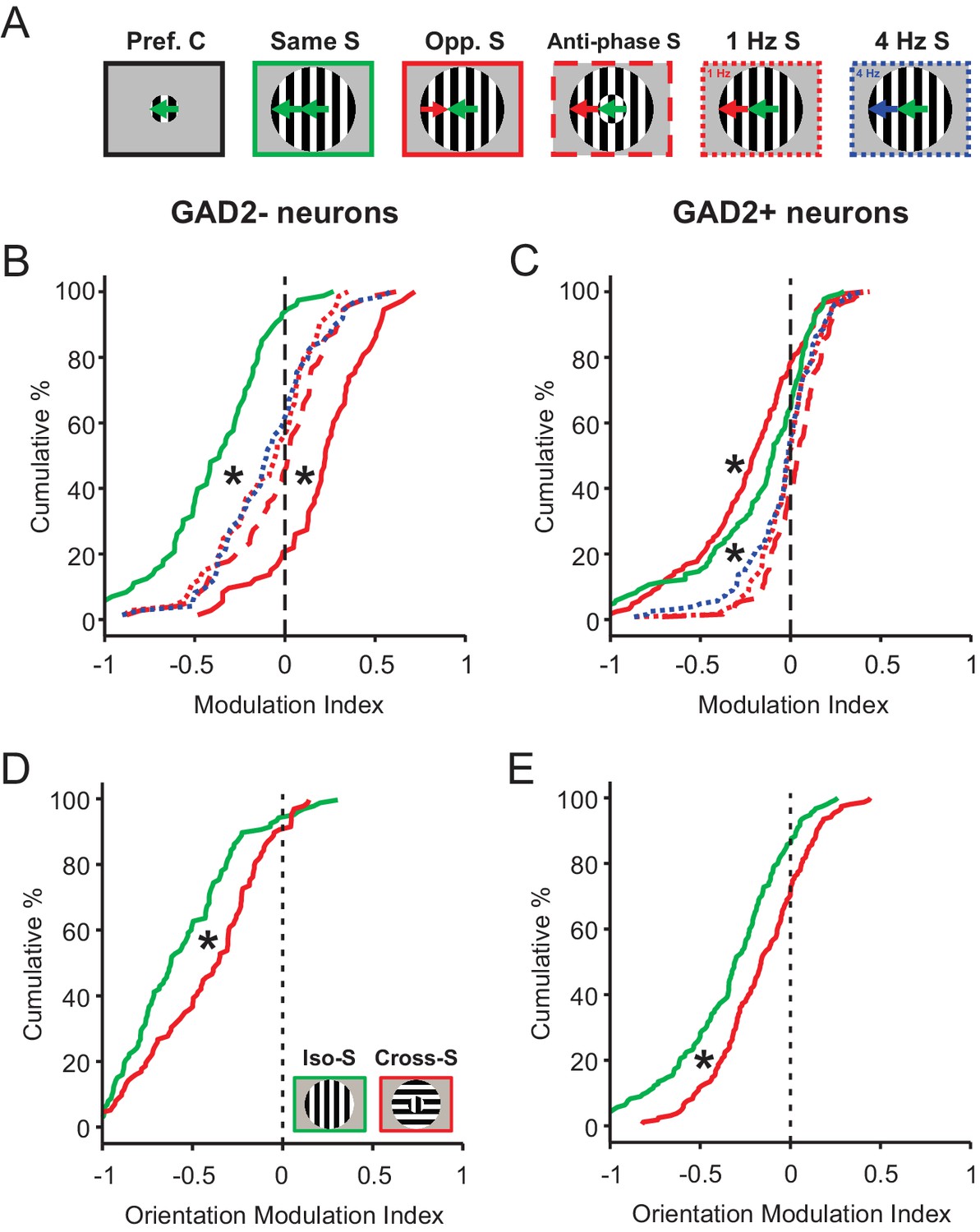
Phase, temporal frequency, and orientation contrasts have a different modulatory effect on sSGS neurons compared to direction contrast.
(A) Visual stimuli used in this set of experiments and analyses, with center gratings presented at individual cells’ preferred directions, either alone (Pref. C, left) or surrounded by different patterns of drifting grating: surround along the same direction, opposite direction, anti-phase along the same direction, and different temporal frequencies (Opp., Opposite; S, Surround). (B–C) Modulation index quantifying how the response to each C-S stimuli differ from that to center grating only. The same color and line styles follow those in A. Plot B is for center-responsive GAD2- neurons (n = 73, 3 mice, KS test, p<0.01 between opposite direction surround and any of the three dotted or dashed lines; and p<0.01 between same direction surround and any of the three dotted or dashed lines). Plot C is for GAD2+ neurons (n = 124, 3 mice, KS test, p<0.01 between opposite direction surround and any of the three dotted or dashed lines, and p<0.01 between same direction surround and any of the three dotted or dashed lines). (D–E) Modulation index for responses to static oriented gratings in center and surround, under iso-surround (green) and cross-surround (red) conditions in center-responsive GAD2- (D, n = 111, 3 mice, KS test, p = 2.5e-4, KS stat = 0.28), and GAD2+ neurons (E, n = 155, 3 mice, KS test, p = 5.8e-4, KS stat = 0.23).
Figure 6 with 2 supplements
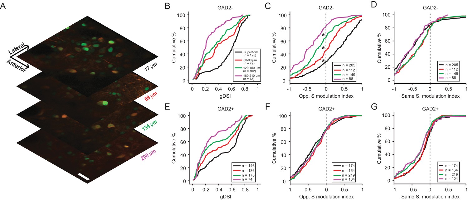
Direction contrast sensitivity declines with depth in the SGS.
(A) Two-photon calcium imaging at different depths of the SGS, using AAV-H2B-GCaMP6s. Shown are neurons expressing H2B-GCaMP6s at four different depths in the SGS of a GAD2-tdTomato mouse. Scale bar is 20 µm. (B) Cumulative distribution of gDSI divided into four depth categories for center-responsive GAD2- neurons (n = 378, 10 mice). The same depth color code applies to panels B-E. (C) Cumulative distribution of the opposite-surround modulation index for center-responsive and center-silent GAD2- neurons (n = 378 + 176=554, 10 mice). (D) Cumulative distribution of the same-surround modulation index for GAD2- neurons (n = 554, 10 mice; p<0.05 between ‘superficial’ and 60 µm, and between 120 µm and 180 µm, KS test). (E–G) Same as in (B–D), but for GAD2+ neurons (n = 534 in D; and n = 534 + 127=661 in E, 10 mice; In G, p<0.05 between 60 µm and 120 µm, KS test).
Figure 6—figure supplement 1
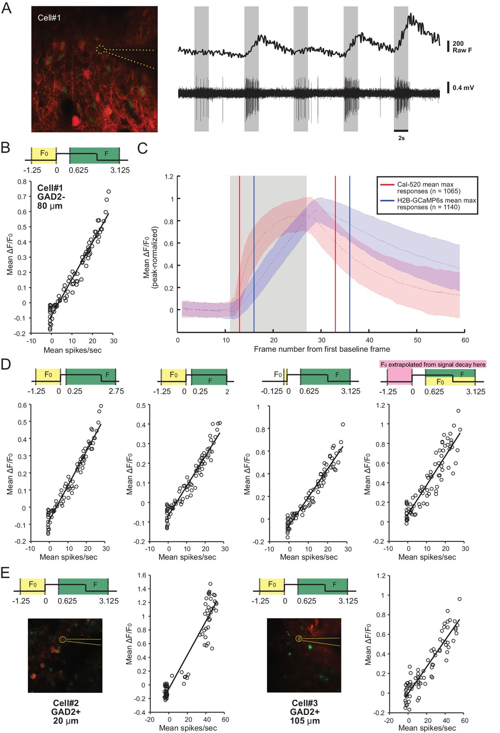
Characterization of H2B-GCaMP6s activity with cell-attached recording.
(A) Example GAD2- neuron patched at a depth of 80 μm (left) and the corresponding raw calcium trace and spiking activity of the same neuron (Cell#1) to the presentation of 5 randomized conditions of the C-S visual stimulus (right). (B) Linear relationship between the ΔF/F0 signal and the corresponding spiking activity for Cell#1. Each data point represents a single trial. (C) Comparison between the response dynamics of Cal-520 and H2B-GCaMP6s by averaging the maximum responses of all cells (i.e. each cell’s response to its preferred C-S combination), after normalization to the peak of each trace (Red, mean and SD of the Cal-520 responses, n = 1065; Blue, mean and SD of the H2B-GCaMP6s responses, n = 1140). The gray shaded region represents the 2 s period of visual stimulus presentation. The red vertical lines delimit the ΔF/F0 window for analyzing Cal-520; the blue vertical lines delimit the ΔF/F0 window for H2B-GCaMP6s. (D) Relationship between ΔF/F0 and spike rate for Cell#1 using four different methods for calculating ΔF/F0. For panels B, D, and E, diagrams on top of each panel represent the different methods for ΔF/F0 calculation. The onset and offset of the stimulus is depicted as a square wave. Time stamps are in seconds, and the yellow and green shaded regions represent the respective time windows for F0 and F that were considered for the calculation of ΔF/F0. For the last panel in D, F0 for every point in F was extrapolated from the signal decay before stimulus onset (pink shaded region). Note that regardless of the method, the relationship between ΔF/F0 and spiking is maintained; the only major difference being the magnitude of ΔF/F0. (E) Relationship between ΔF/F0 and spike rate for two more example cells (Cell#2, left; Cell#3, right), using the adopted ΔF/F0 calculation method in this study.
Figure 6—figure supplement 2
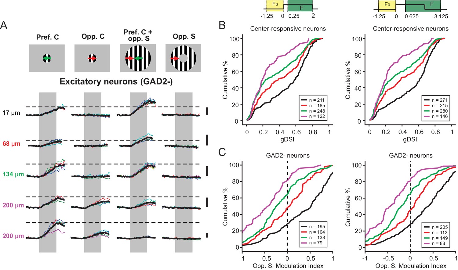
Varying the time window of H2B-GCaMP6s signal analysis does not impact the main findings.
(A) Calcium signal of 5 GAD2- neurons in response to four chosen conditions of the C-S stimulus. The depth of each neuron in the SGS is specified to the left. Figure conventions are the same as in Figures 1C and 3A. (B) Comparison in the distribution of the gDSI using two different ΔF/F0 calculation methods, showing very similar trends. The ΔF/F0 calculation methods are described at the top and apply to the corresponding panels in both B and C below. (C) The distribution of the modulation index of GAD2- cells by the opposite surround is also preserved under those two ΔF/F0 calculation methods. The depth color code in panels B and C is the same as in Figure 4B–E.
Figure 7 with 1 supplement
Relationship between surround modulation and direction selectivity.
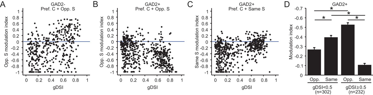
(A–B) Relationship between the opposite-surround modulation index and gDSI for center-responsive GAD2- neurons (A, n = 378, 10 mice) and GAD2+ neurons (B, n = 534, 10 mice) at all depths combined. (C) Relationship between the same-surround modulation index and gDSI for the same cells in B. (D) Modulation index by same or opposite surround for GAD2+ neurons, separated into two gDSI categories (gDSI < 0.5, n = 302; gDSI ≥ 0.5, n = 232, 10 mice. Data are presented as mean ± s.e.m. * represents p<0.01, Mann-Whitney U-test).
Figure 7—figure supplement 1
Relationship between surround modulation and direction selectivity of sSGS neurons imaged by Cal-520.
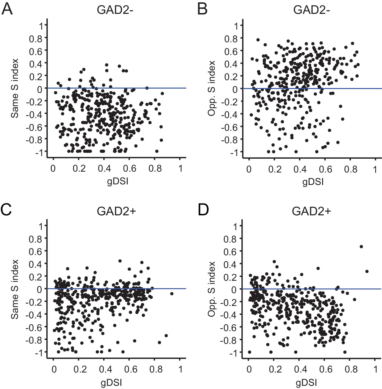
(A–B) Relationship between the modulation index and gDSI for center-responsive GAD2- neurons under same-direction surround (A, r = −0.05, p=0.33) and opposite-direction surround (B, r = 0.20 p=1.0e-4). (C–D) Relationship between the modulation index and gDSI for center-responsive GAD2+ neurons (n = 379 cells, 9 mice) under same-direction surround (C, r = 0.24, p=1.5e-6), and under opposite-direction surround (D, r = −0.35 p=2.0e-12).
Additional files
-
Source data 1
The Matlab workspace used to generate Figures 1–4 are included in this ZIP file.
- https://doi.org/10.7554/eLife.35261.016
-
Source data 2
The Matlab workspace used to generate Figure 5 are included in this ZIP file.
- https://doi.org/10.7554/eLife.35261.017
-
Source data 3
The Matlab workspace used to generate Figures 6–7 are included in this ZIP file.
- https://doi.org/10.7554/eLife.35261.018
-
Transparent reporting form
- https://doi.org/10.7554/eLife.35261.019
Download links
A two-part list of links to download the article, or parts of the article, in various formats.
Downloads (link to download the article as PDF)
Open citations (links to open the citations from this article in various online reference manager services)
Cite this article (links to download the citations from this article in formats compatible with various reference manager tools)
Bidirectional encoding of motion contrast in the mouse superior colliculus
eLife 7:e35261.
https://doi.org/10.7554/eLife.35261


