First spikes in visual cortex enable perceptual discrimination
- University of California, San Diego, United States
- University of California, San Francisco, United States
- Allen Institute for Brain Science, United States
- Howard Hughes Medical Institute, University of California, San Francisco, United States
Figures
Figure 1 with 3 supplements
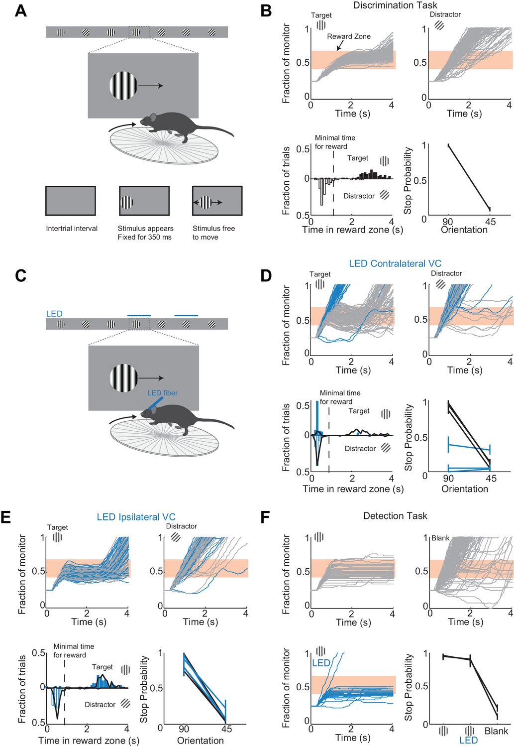
A virtual foraging behavior that depends on visual cortex.
(A) Behavioral setup. The mouse is rewarded for stabilizing the target at the center of the monitor for about a second. (B) Example session for a trained mouse. Top. Grey lines are individual stimulus trajectories. Orange shaded area is the reward zone. Note different trajectories of target versus distractor stimuli. Bottom left. Distribution of the times spent in the reward zone for target (filled bars) and distractor stimuli (empty bars). Bottom right. The probability that mice place the object in the reward zone for at least the minimal time for reward (stop probability) depends on the identity of the grating. Here and further, error bars are 95% confidence intervals. (C) Behavioral setup as above but visual cortex (VC) is silenced before the appearance of the stimulus and for the duration of the trial on a randomly interleaved fraction of trials. (D) Behavioral performance depends on contralateral VC. Same conventions as in (B). Top. Example mouse. Stimulus trajectories during cortical silencing are in blue. This particular mouse systematically overshot the reward zone when centering the target and subsequently moved backwards to bring the target back in the reward zone. Bottom left. Distribution of times spent in reward zone. Black: control; Blue: VC silencing. Bottom right. Stop probability under control conditions (black) and during VC silencing (blue). Individual lines are individual mice (n = 3). (E) Behavioral performance is not affected by silencing ipsilateral VC. Same conventions as in (D). (F) V1 is not required to express the decision in a detection task. Mice trained with one stimulus only (the target) are rewarded for stabilizing it at the center of the monitor. Top, Bottom left. Example mouse. Stimulus trajectories during cortical silencing are in blue. Same conventions as (B). A blank is defined as the absence of a target at regularly spaced distances. Bottom right. Stop probability for two mice (individual lines).
Figure 1—figure supplement 1
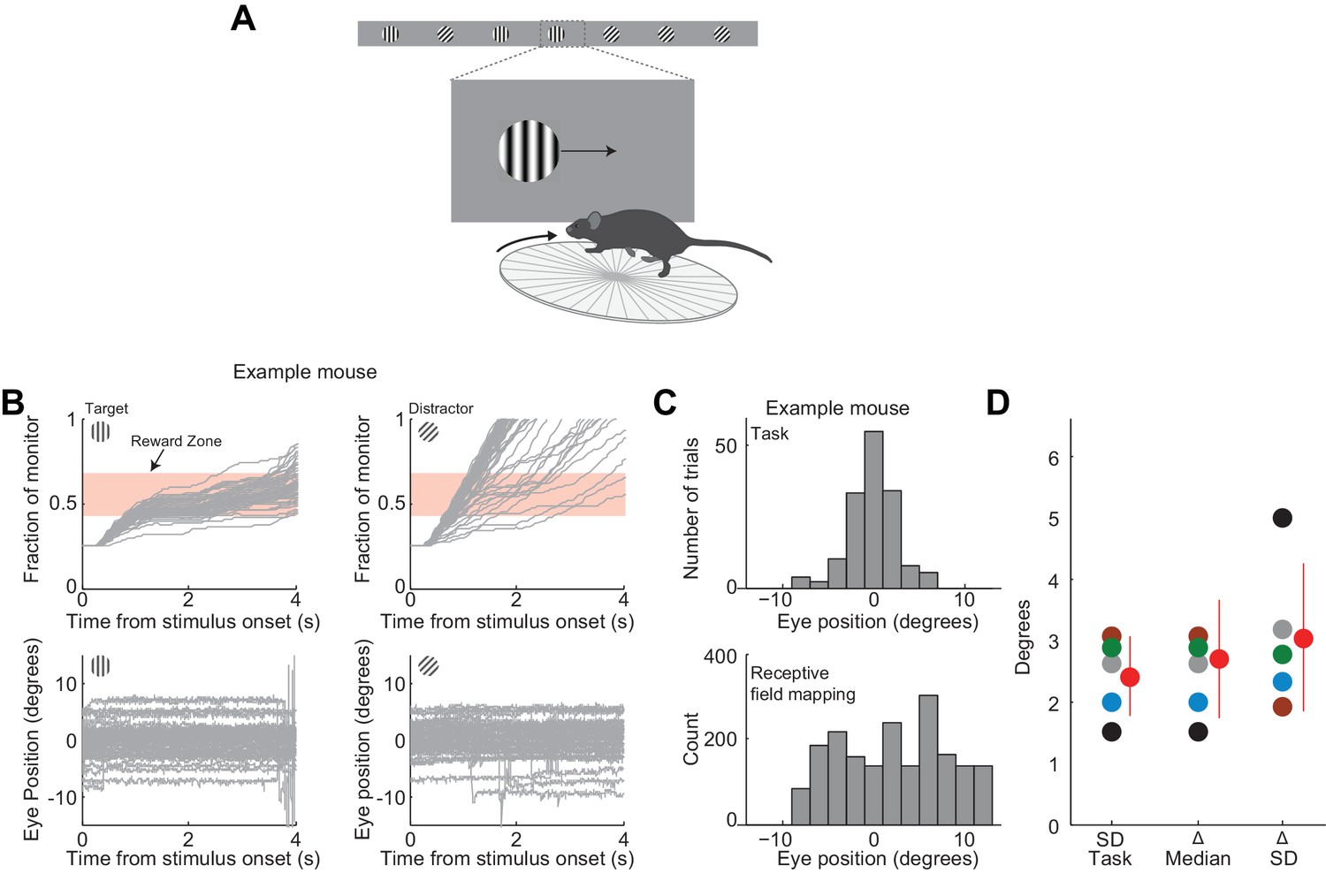
Eye movements in trained mice.
(A) Behavioral setup as in Figure 1A. (B) Eye positions in an example session in a trained mouse. Top. Grey lines are individual stimulus trajectories. Bottom. Grey lines are horizontal positions of the right eye (pupil center) during individual stimulus presentations (Top). Zero degrees is the mean eye position. Note that the animal does not follow the stimulus with their gaze (following the initial 350 ms, when the stimulus was movable by the animal, the mean eye position remained very similar to the initial 350 ms: difference in medians: 0.3±0.4 degrees, mean ± std across 5 mice). (C) Top. Distribution of eye positions across trials during the task for the example session in A. Each trial, eye position was quantified as the average position over 0–350 ms relative to stimulus onset. Bin size is two degrees. Bottom. Distribution of eye positions outside of the task, during stimulus presentation used for receptive field mapping (measured immediately following the task; see Methods). Eye position was quantified as the average position over 350 ms time bins. Zero degrees corresponds to the same position as during the task. Note that, while eye position is more variable during receptive field mapping, the average eye position is similar. (D) Variability of eye positions in individual mice: variability of eye position during the task (SD Task), difference in the median eye position during receptive field mapping and during the task (Δ Median), and difference in variability of eye position during receptive field mapping and during the task (Δ SD). Different colors indicate different mice (n = 5, one session per mouse). Grey indicates example mouse in (B) and (C). Red circle and line indicates mean and SD across mice.
Figure 1—figure supplement 2
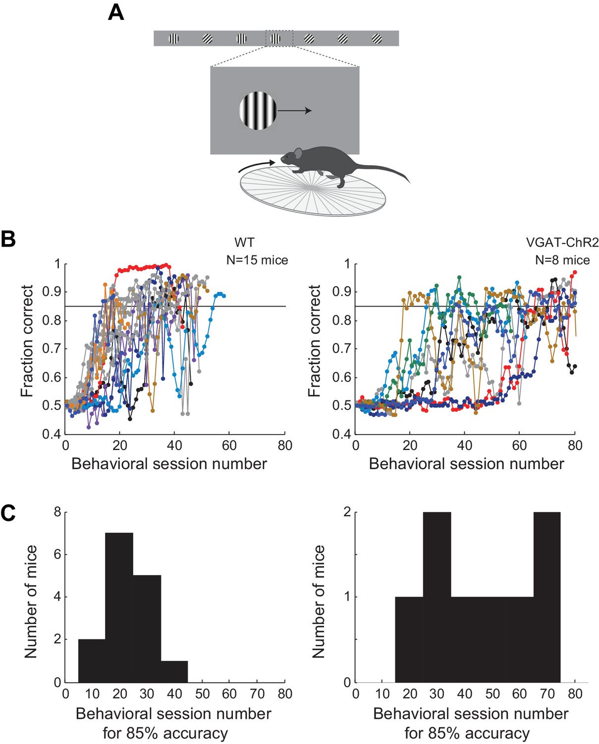
Learning curves for wild type and transgenic mice.
(A) Behavioral setup. (B) Probability of a correct choice for the different behavior sessions over the course of training for wild type mice (left, subset of mice trained for subsequent electrophysiology recordings, all mice shown in the main figures are included) and transgenic mice (right, subset of mice trained for subsequent optogenetic silencing or electrophysiology recordings, 8/9 mice shown in the main figures are included; for 1/9 mice the initial training data was corrupted). Sessions lasting <10 min were excluded. Probability of a correct choice for a given session is the average of the probability of a correct choice in a 3-session sliding window centered on the shown trial. Individual lines are individual mice. (C) Distribution of the number of training sessions that it takes mice to reach an overall accuracy of 85% correct.
Figure 1—figure supplement 3
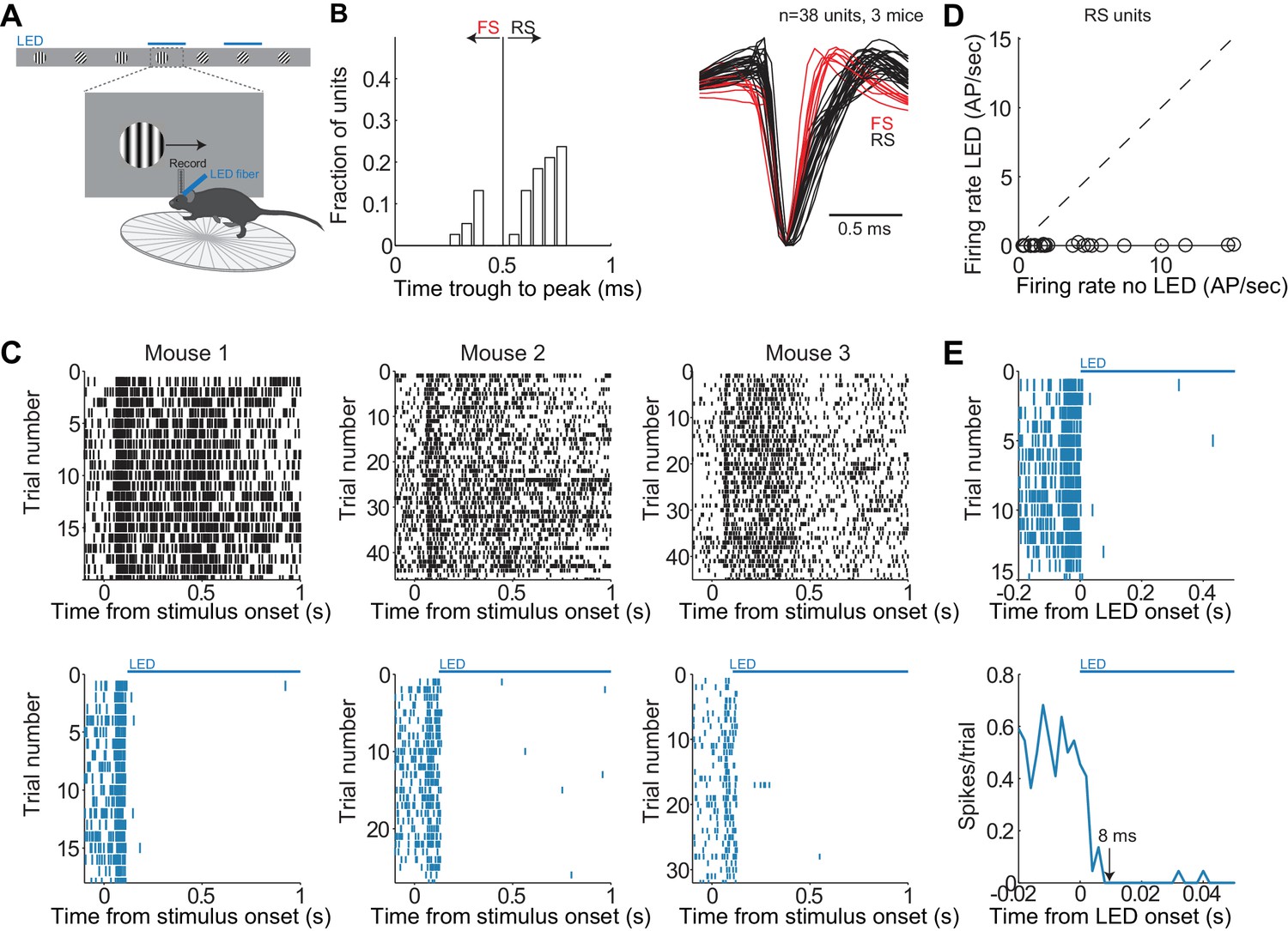
Reversible, rapid and complete silencing of V1.
(A) Experimental set up as in Figure 1C. (B) Distribution of the time from trough to peak in the average waveform of the action potential across single units (n = 3 mice). Single units are labelled as regular spiking (RS, black lines) or fast spiking (FS, red lines) depending on their time of trough to peak. (C) Reversible and complete silencing of V1. Top. Raster plots (each dot is an action potential) for three mice including all isolated single units (all layers) for trials under control conditions (no LED) aligned at stimulus onset. Bottom. Same as above but for trials with LED illumination. LED and control trials were randomly interleaved. LED onset was approximately at 120 ms after stimulus onset. (D) Firing rate of individual RS units computed from 130 ms to 1 s following stimulus onset under control conditions plotted against firing rate during LED illumination. (E) Rapid silencing of V1. Top. Raster plot (each dot is an action potential) for all RS units from all three mice for trials with LED illumination aligned at the time of LED onset. Bottom. Peri-event time histogram from all isolated single units (2 ms bins) for trials with LED illumination. Arrow indicates time when the firing rate drops to zero.
Figure 2
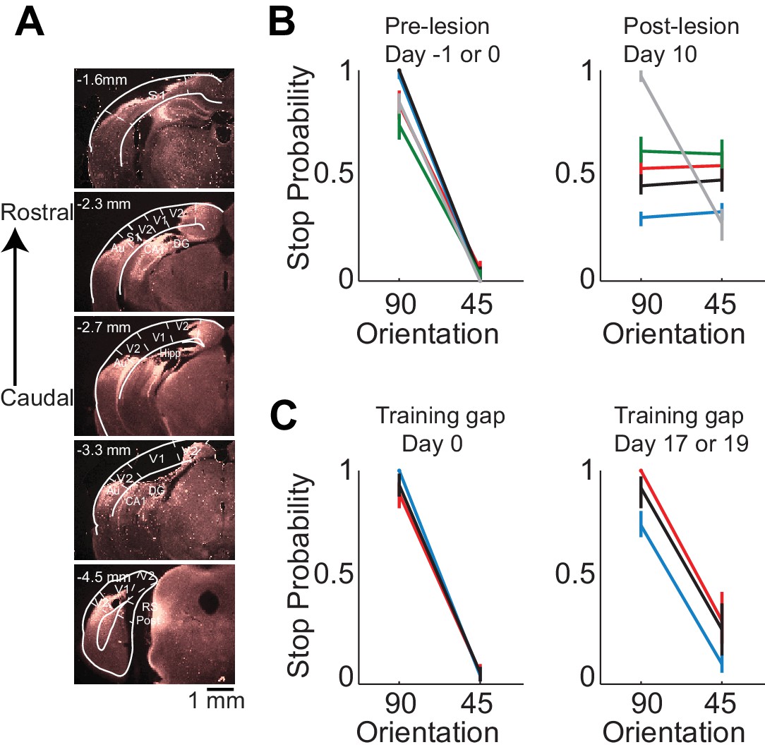
Lesion of visual cortex disrupts behavior.
(A) Coronal brain sections showing the extent of lesion for an example mouse (black in (B) and (C), 100 µm sections, images of background fluorescence, see Methods for summary of all mice). Outline of the different brain areas is from the Paxinos and Franklin brain atlas (Paxinos and Franklin, 2007). Distances are relative to bregma. The retinotopic location in V1 corresponding to the stimulus in the initial 350 ms is ~3 mm from bregma and 2.3 mm from midline. Note the absence of V1 (black). (B) Stop probability for the target and distractor stimulus when mice performed the task (left) just before the lesion of visual cortex (day 0) or the previous day (day −1) and (right) when mice performed the task 10 days after the lesion of visual cortex. Individual lines are individual mice. Each color represents the same mouse in all panels. All mice except the one displayed in grey had lesions in the left visual cortex (contralateral to the stimulus); the one in grey had a lesion in the right visual cortex. Error bars are 95% confidence intervals. (C) Stop probability for 3 of the mice in (B), (left) just before the gap in training (day 0), and (right) after the gap in training (day 17 or day 19 without training).
Figure 3 with 2 supplements
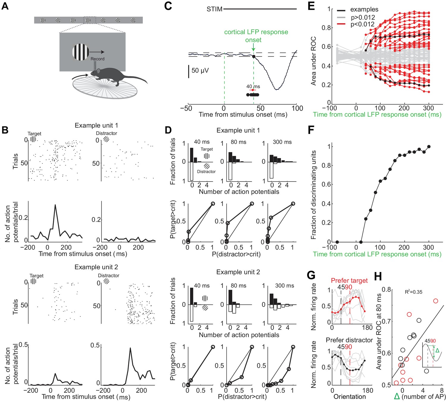
Individual neurons can discriminate within 80 ms from onset of cortical response.
(A) Experimental setup as in Figure 1A but with recording from primary visual cortex. (B) Responses of two example units recorded simultaneously. Top. Raster plot. Black dots are action potentials. Bottom. Peristimulus time histogram (PSTH). The number of action potentials per trial is calculated in 25 ms bins. (C) Estimation of the onset of cortical response. The onset of cortical response is defined for each mouse as the earliest deflection in the local field potential following stimulus onset. Dashed lines indicate three standard deviations from baseline. Black circles indicate onset of cortical response in nine mice. Red circle and line are the mean and standard deviation across mice. (D) Receiver operating characteristic (ROC) analysis for the two example units in (B). Top. Distribution of action potentials across trials for target (black bars) and distractor stimuli (white bars) at three different intervals after the onset of cortical response. Bottom. ROC curve for each graph on top. (E) Summary of areas under ROC for 72 units. Area under ROC for individual units (individual lines) depends on the interval from cortical onset. Black: example units in (C) and (D). For each unit at each interval starting at cortical response onset, statistical significance for the separation of the distributions of the number of action potentials for the target versus distractor was assessed using Wilcoxon ranksum test and the Benjamini-Hochberg correction for multiple comparisons (p<0.012). (F) The fraction of discriminating units discriminating at a particular interval increases with increasing time from cortical response onset. A unit is defined as discriminating if by 300 ms p<0.012. (G) Experimental set up as in (A) but stimulus position is always fixed, mouse is not rewarded, and the grating is drifting. Grey lines are orientation tuning curves for individual discriminating units preferring the target (top) or the distractor (bottom) during the task. Colored line is the mean across units. (H) The area under ROC over the initial 80 ms after cortical onset during the task is plotted against the difference in the number of action potentials in response to passively viewed stimuli of 45° and 90°. Circles are individual discriminating units (p<0.012, Wilcoxon ranksum test) that prefer target (red) or distractor (black). R2 is the fraction of the variance explained by the linear fit to the data.
Figure 3—figure supplement 1
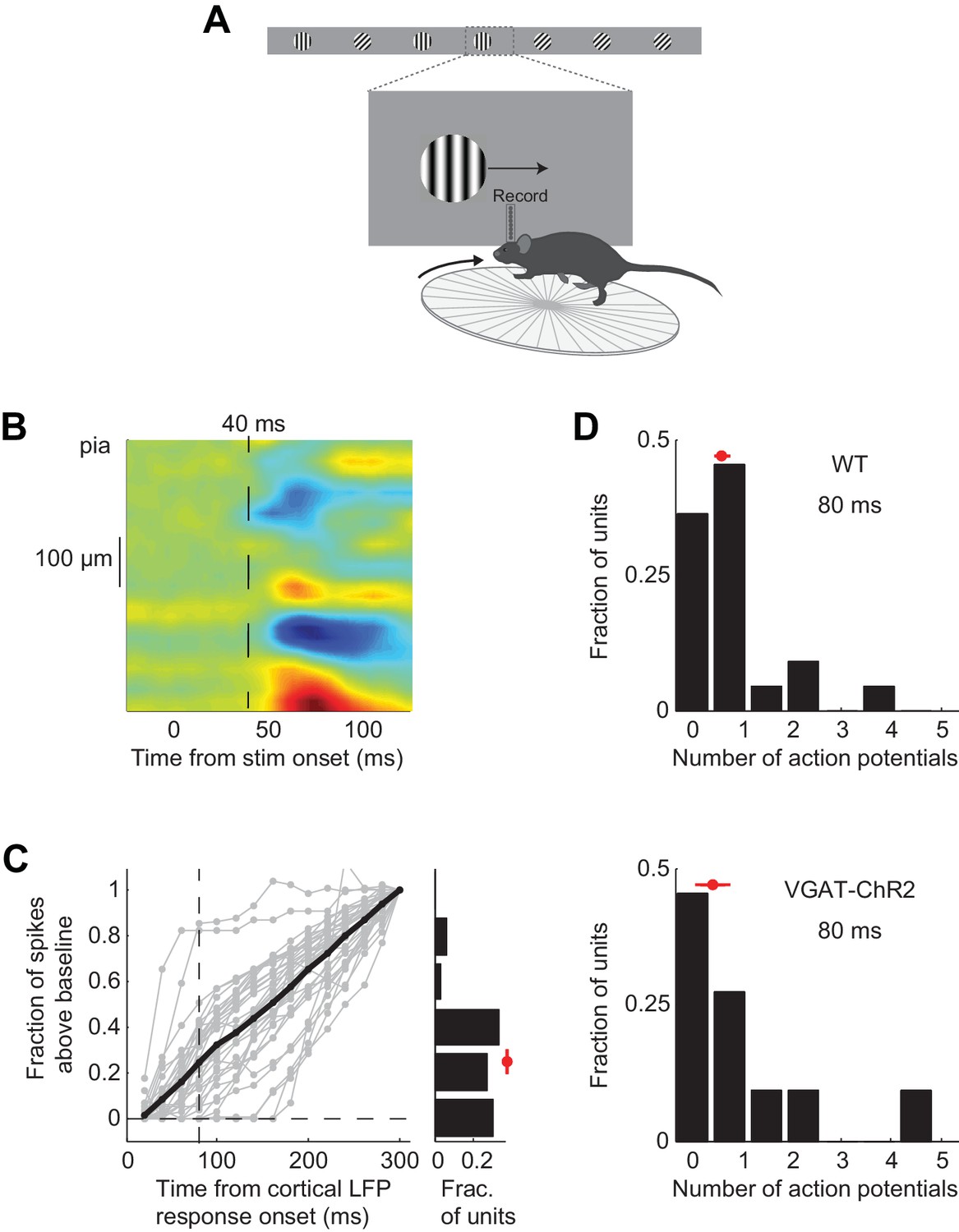
Characterization of V1 recordings during behavior.
(A) Experimental setup as in Figure 3A. (B) Average current source density for five mice (see Methods). Blue indicates current sinks; red indicates current sources. The top sink is layer 4. 40 ms indicates the average onset of the cortical response across mice (see Figure 3C). (C) Fraction of stimulus elicited spikes at different time intervals relative to 300 ms following onset of cortical response. Grey lines are individual discriminating units; black line is the mean. If a unit was suppressed below baseline, the value for spikes above baseline was set to zero. Vertical dotted line marks 80 ms. Right. Distribution of the fraction of stimulus elicited spikes at 80 ms following onset of cortical response for all discriminating units. By 80 ms discriminating units fire 25 ± 4% of the total spikes. (D) Distribution of the number of action potentials fired over the initial 80 ms following onset of the cortical response for discriminating units recorded from wild type mice (top, n = 5 mice) or VGAT-ChR2 mice (bottom, n = 4 mice). The two distributions are not significantly different (p=0.95, Wilcoxon rank sum test). Red circle and line through it indicate median and sem, respectively.
Figure 3—figure supplement 2
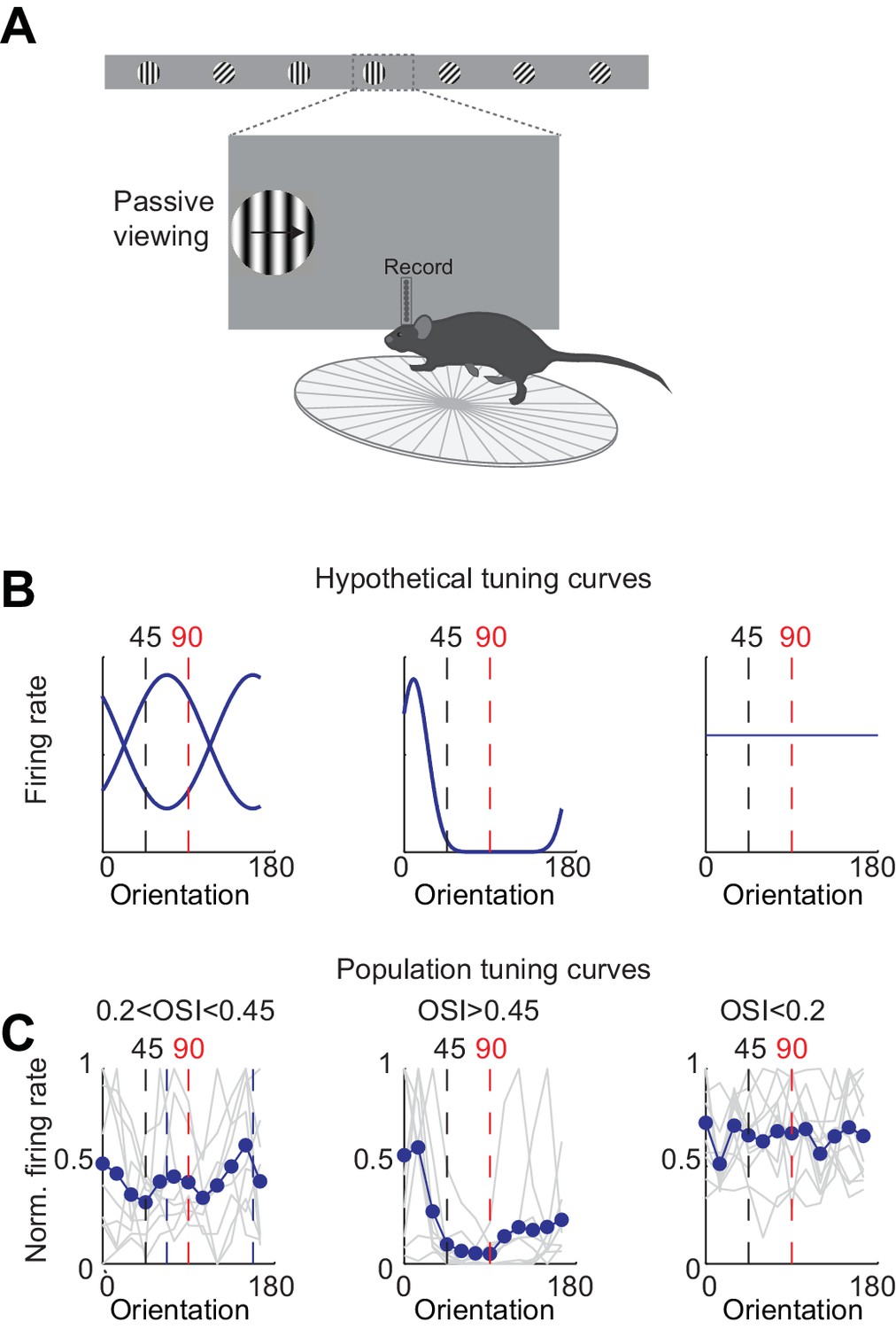
Tuning curves for units that do not discriminate.
(A) Experimental set up as in Figure 3A but the stimulus position is always fixed, mouse is not rewarded, and the grating is drifting. (B) Example hypothetical tuning curves for units that do not discriminate. Left. Peak of tuning curve is in the middle of distractor (45°) and target (90°; i.e. 67.5° and 157.5°).Middle. Narrow tuning curve with peak away from 45° and 90°. Right. Flat tuning curve. (C) Population tuning curves. Individual units (grey lines) were grouped according to their orientation selectivity index (OSI). Blue lines are the population mean.
Figure 4
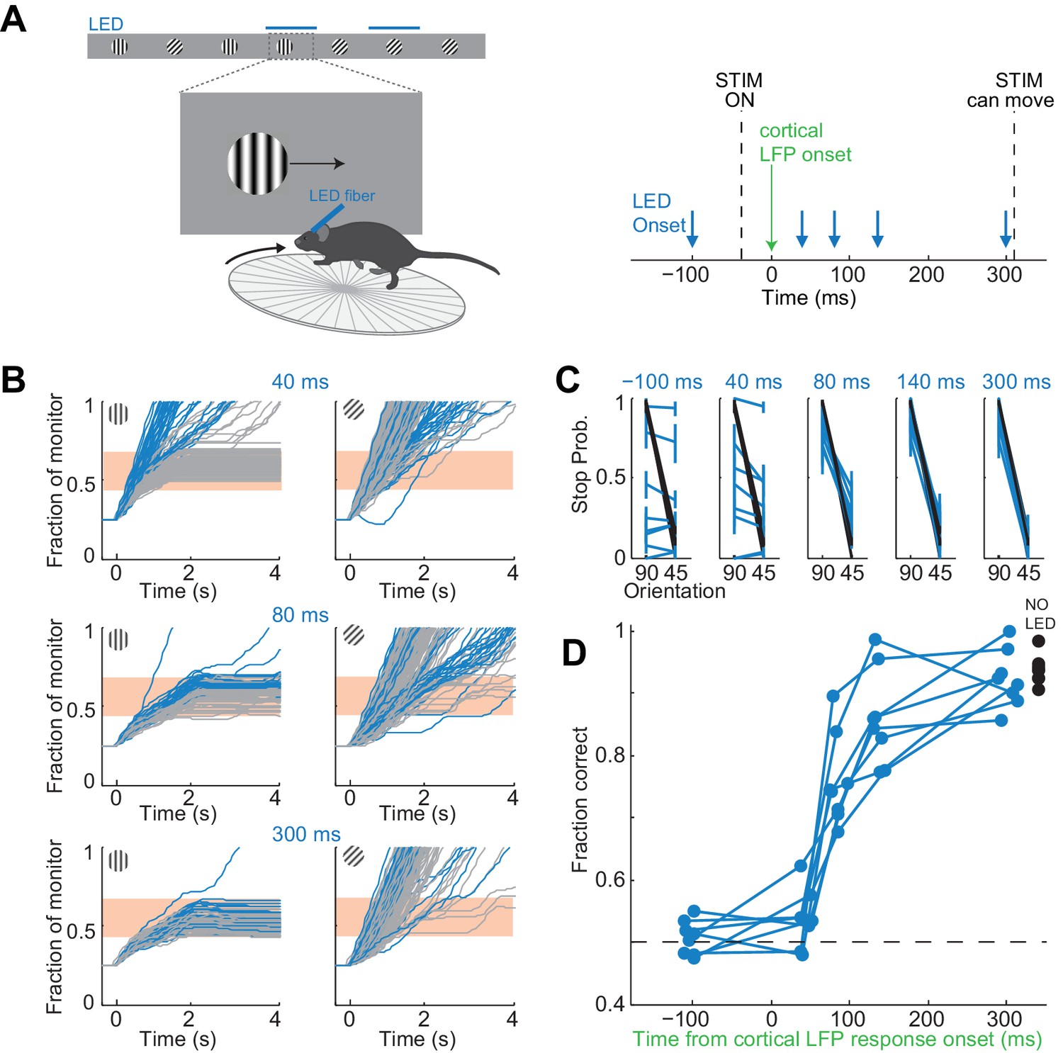
It takes visual cortex 80 ms to enable perceptual discriminations.
(A) Left: Experimental setup. Right: Arrows indicate the onset of LED illumination. Each interval was tested in separate behavioral sessions. (B) Example mouse. Stimulus trajectories during cortical silencing (blue) and under control conditions (gray) for three different LED illumination onset latencies (40 ms; 80 ms; 300 ms) relative to the onset of the cortical response. Individual lines are individual trials. (C) Summary of stopping probability for eight mice. Black: control; Blue: cortical silencing. Times indicate the LED illumination onset after onset of the cortical response. Individual lines are individual mice. Error bars are 95% confidence intervals. Note that behavioral performance during cortical silencing increases with increasing LED onset. (D) Probability of a correct choice during cortical silencing (blue) depends on the onset of LED illumination relative to the onset of the cortical response. Individual lines are individual mice. Black circles indicate probability correct for individual mice for trials with no cortical silencing.
Figure 5
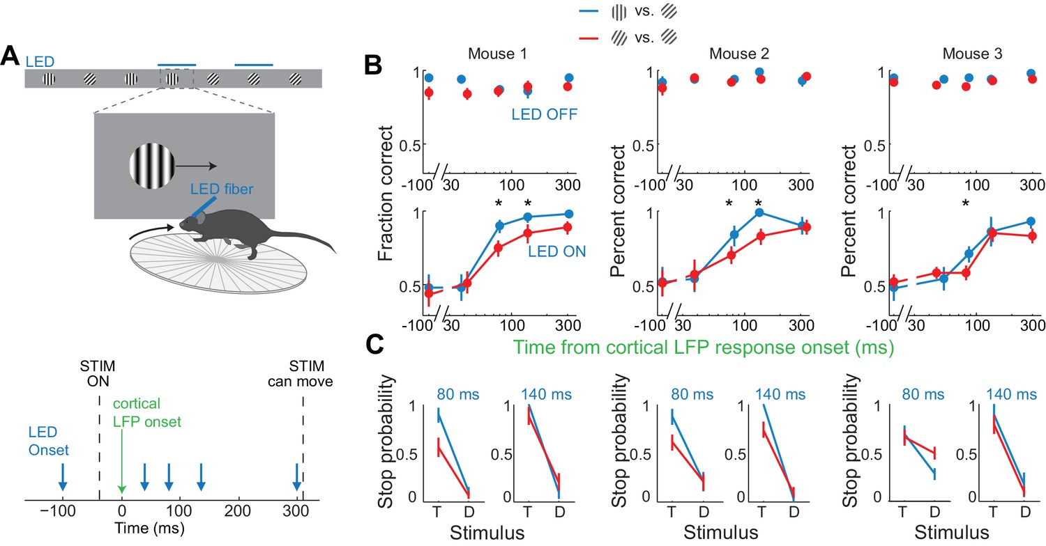
Discrimination accuracy when V1 is active for only 80 ms is sensitive to the difficulty of the task.
(A) Experimental setup as in Figure 4A. (B) Probability of a correct choice for (top) control trials and for (bottom) trials with cortical silencing for three mice first trained in the main task (blue, target: 90°, distractor: 45°) and then in the harder discrimination task (red, target: 60°, distractor: 45°). Error bars are 95% confidence intervals. Asterisks indicate significant difference in the choice accuracies in the two tasks (p=0.001–0.018, Wilcoxon ranksum test on choice data). (C) Stop probability for the target stimulus (T) and the distractor stimulus (D) for two intervals from (B), left, when cortex is silenced at 80 ms or, right, 140 ms following onset of cortical response.
Figure 6 with 1 supplement
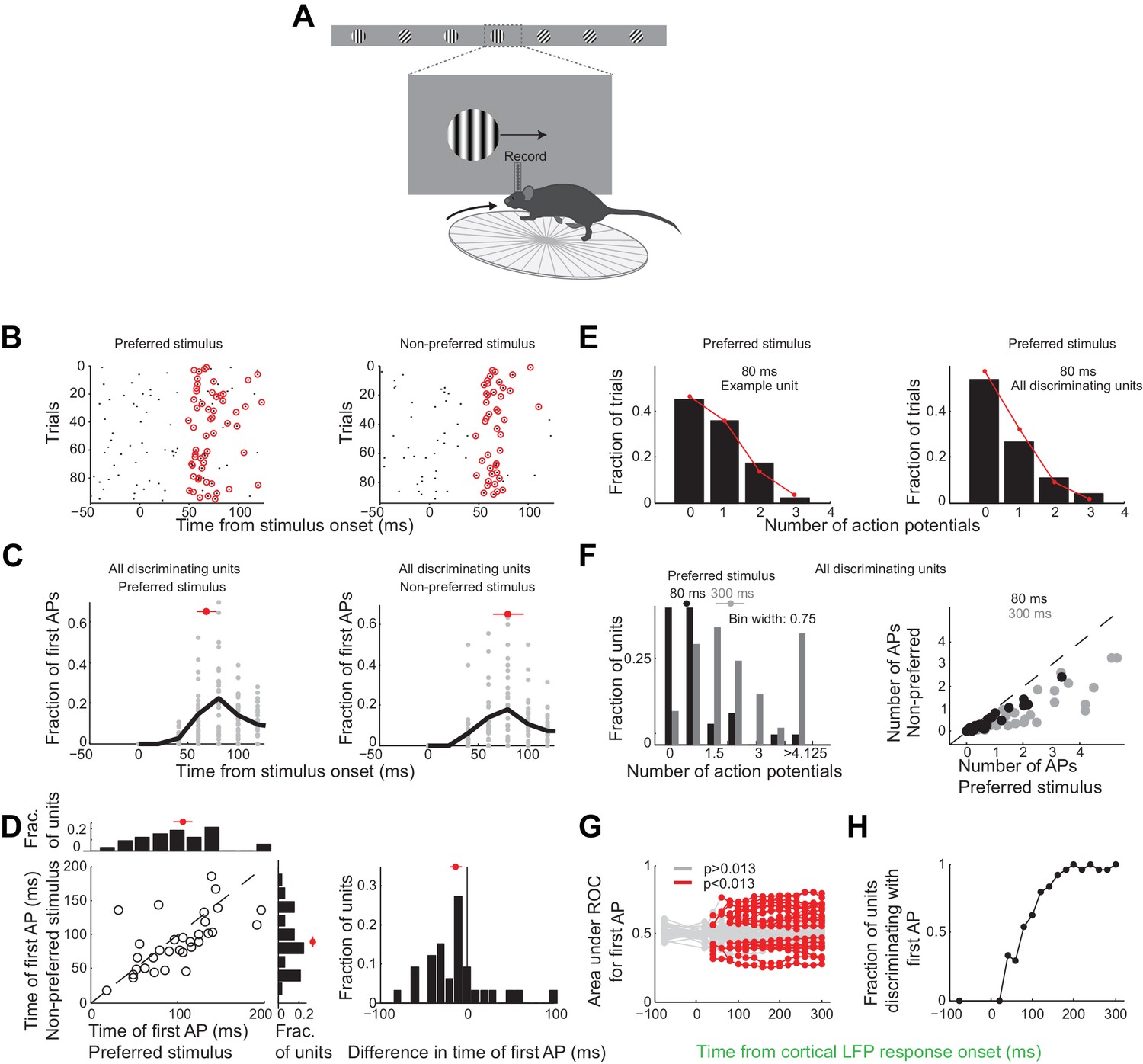
Neurons usually fire only their first action potential in the initial 80 ms.
(A) Experimental setup as in Figure 3A. (B) Raster plot (APs, black dots) for an example unit for preferred (left) versus the non-preferred stimulus (right). Red circles indicate the first AP in each trial after the onset of the cortical response. (C) The distribution of times of the first AP for individual discriminating units (grey circles, time bins of 20 ms) for those trials in which the first AP occurred within the initial 300 ms following the onset of the cortical response, for (left) the preferred and (right) the non-preferred stimulus. Black line is the mean across units. Red circle and line through are the median and SEM, respectively. (D) Mean of times of the first AP across trials for individual discriminating units (circles; same trials and window as in C) plotted for the preferred stimulus versus the non-preferred stimulus. Top. Distribution of the mean times for the preferred stimulus. Right. Distribution of the mean times for the non-preferred stimulus. Red circle and line through are the median and SEM, respectively. Right panel. Distribution of the difference in the mean time of the first AP for the preferred and the non-preferred stimulus for all discriminating units. Red circle and line through are the median and SEM, respectively. (E) The distribution of the number of APs across trials for the preferred stimulus for the initial 80 ms after cortical onset for (left) the example unit in (B) and for (right) all discriminating units approximates a Poisson distribution predicted from the mean number of APs (red line). (F) Left panel. The distribution of the number of action potentials (mean across trials) across discriminating units is shown for the preferred stimulus over the initial 80 ms (black) and 300 ms (grey). Last bin also includes units that fired more than 5 APs. Circle and line through are the median and SEM, respectively. Right panel. The number of APs (mean across trials) for individual discriminating units (circles) for the preferred versus the non-preferred stimulus over the initial 80 ms (black) and the initial 300 ms (grey). (G) Area under ROC for individual units (individual lines), based only on the first AP after cortical onset on each trial plotted against the interval from the onset of the cortical response. Statistical significance was assessed same as in Figure 3E. (H) Fraction of discriminating units discriminating depends on the interval from cortical onset. A unit is defined as discriminating if by 300 ms p<0.013.
Figure 6—figure supplement 1

Comparison of neural and behavior discrimination.
(A) Experimental setup as in Figure 3A. (B) Area under ROC curve as a function of time from cortical onset for a 'pooling neuron', which for each trial has all the spikes of N units that are randomly drawn from a pool of all discriminating units (see Methods). Each line is the average of the areas under ROC for 10 different pools of discriminating units. Errorbars are sem. For each area under ROC curve, at each interval, statistical significance for the separation in the distribution of number of action potentials for the target versus the distractor was assessed using Wilcoxon ranksum test (p<0.05). f is at each time interval the fraction of 'pooling neurons' with p<0.05. Blue line is the average probability of a correct choice for all the mice in Figure 4D. (C). Same as B but for all units.
Videos
Video 1
Video of a trained mouse performing the task.
The mouse is rewarded with water for stabilizing the target (90 degree grating) in the center of the monitor. There is no reward or punishment for the distractor (45 degree grating). The speed of the stimulus is proportional to the running speed. Note that the stimulus is frozen (i.e. insensitive to the rotation of the treadmill) for 350 ms following its appearance.
Additional files
-
Supplementary file 1
Parameters for the behavioral task for each of the mice included in the main experiments.
Hold time is the minimal time that the target stimulus has to spend in the reward zone for a reward to be available. Track gain is the stimulus displacement on the monitor (cm)/running distance (cm). Target probability is the fraction of stimuli that are the target stimulus (stimuli are randomly interleaved).
- https://doi.org/10.7554/eLife.34044.015
Download links
A two-part list of links to download the article, or parts of the article, in various formats.
Downloads (link to download the article as PDF)
Open citations (links to open the citations from this article in various online reference manager services)
Cite this article (links to download the citations from this article in formats compatible with various reference manager tools)
First spikes in visual cortex enable perceptual discrimination
eLife 7:e34044.
https://doi.org/10.7554/eLife.34044


