Lamina-specific cortical dynamics in human visual and sensorimotor cortices
- University College London, United Kingdom
- Cardiff University, United Kingdom
- Birkbeck College, University of London, United Kingdom
Figures
Figure 1
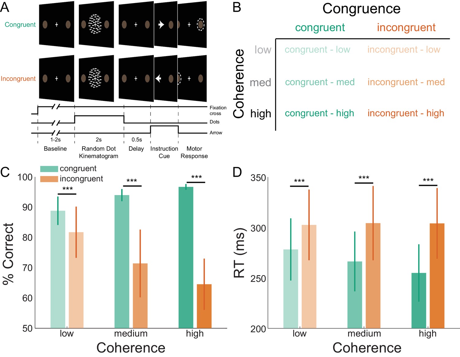
Task structure and participant behavior.
(A) Each trial consisted of a fixation baseline (1 – 2 s), random dot kinematogram (RDK; 2 s), delay (0.5 s), and instruction cue interval, followed by a motor response (left/right button press) in response to the instruction cue (an arrow pointing in the direction of the required button press). During congruent trials the coherent motion of the RDK was in the same direction that the arrow pointed in the instruction cue, while in incongruent trials the instruction cue pointed in the opposite direction. (B) The task involved a factorial design, with three levels of motion coherence in the RDK and congruent or incongruent instruction cues. Most of the trials (70%) were congruent. (C) Mean accuracy over participants during each condition. Error bars denote the standard error. Accuracy increased with increasing coherence in congruent trials, and worsened with increasing coherence in incongruent trials. (D) The mean response time (RT) decreased with increasing coherence in congruent trials (***p<0.001). See Figure 1 – source data for raw data.
-
Figure 1—source data 1
Accuracy and response time data.
- https://doi.org/10.7554/eLife.33977.004
Figure 2 with 1 supplement

Cross-session reproducibility.Topographic maps (left column), event-related fields (ERFs, middle column), and time-frequency decompositions (right column).
(A) aligned to the onset of the random dot kinematogram (RDK), (B) aligned to onset of the instruction cue, (C) aligned to the participant’s response (button press). Data shown are for a single representative participant, with four sessions recorded on different days spaced at least a week apart (each including three, 15 min blocks with 180 trials per block). The white circles on the topographic maps denote the sensor from which the ERFs in the middle are recorded. Each blue line in the ERF plots represents a single session (average of 540 trials), with shading representing the standard error (within-session variability) and the red lines showing the time point that the topographic maps are plotted for (150 ms for the RDK and instruction cue, 35 ms for the response). The insets show a magnified view of the data plotted within the black square. The time-frequency decompositions are baseline corrected (RDK-aligned: [−500, 0 ms]; instruction cue-aligned: [−3 s, −2.5 s]; response-aligned: [−500 ms, 0 ms relative to the RDK]) and averaged over the sensors shown in the insets. See Figure 2 – source data for raw data.
-
Figure 2—source data 1
Topographic, ERP, and time-frequency data for a representative participant across four recording sessions.
- https://doi.org/10.7554/eLife.33977.007
Figure 2—figure supplement 1
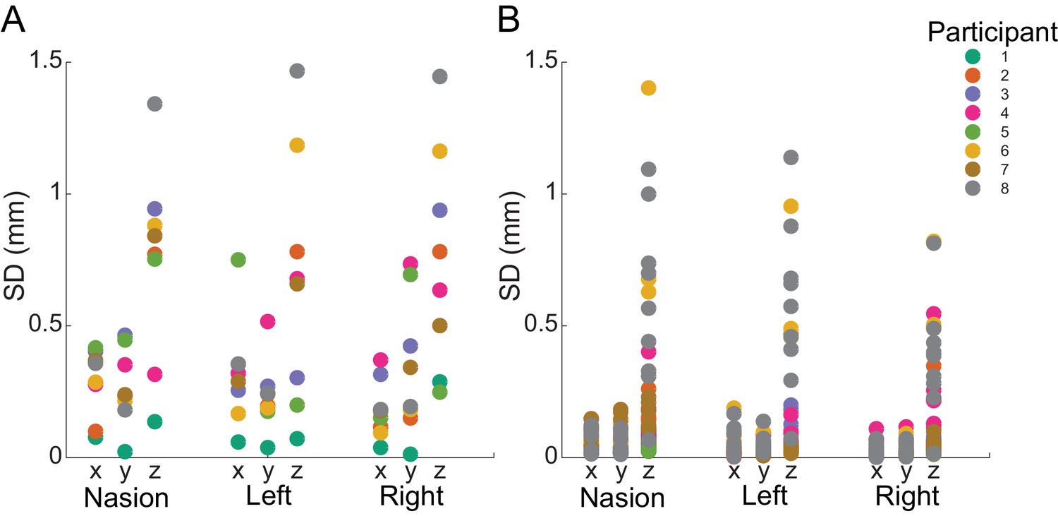
Within- and between-block fiducial coil variability.
(A) Standard deviation of absolute fiducial coil locations for each participant across blocks (with three 15 min blocks per session). Co-registration error between blocks was <1.5 mm for any coil in any dimension. (B) Standard deviation of absolute coil locations for each participant within each block. Movement was <0.5 mm in the x and y dimensions and <1.5 mm in the z dimension for each coil.
Figure 3
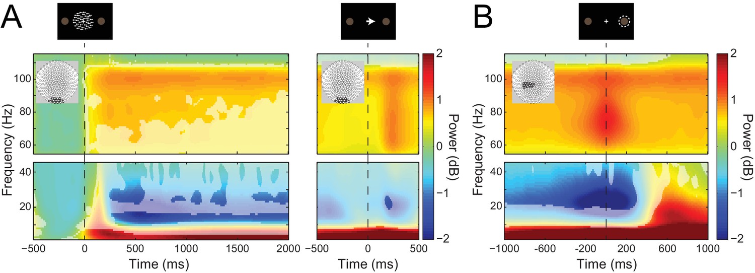
Visual and sensorimotor sensor-level activity.
(A) Time-frequency representations of activity from sensors overlying visual cortex (shown in insets), aligned to the onset of the RDK (left) and the instruction cue (right). Data were baseline-corrected ([−500, 0 ms] relative to the onset of the RDK), and averaged over participants. Overlaid is a mask in which pixels where power is significantly changed from baseline are transparent, revealing the underlying time-frequency power. After the onset of the RDK, there is a sustained decrease in alpha, and increase in gamma activity, followed by a burst of gamma after the instruction cue. (B) Time-frequency representation of movement-related activity from sensors overlying contralateral sensorimotor cortex (shown in inset), aligned to the response, and baseline corrected ([−500, 0 ms] relative to the onset of the RDK), and averaged over participants. As in A, the mask overlaid reveals pixels with a significant change from baseline. There is a decrease in beta power prior to the motor response, followed by a beta rebound after the response, and a burst of gamma power aligned to the time of the response. See Figure 3 – source data for raw data.
-
Figure 3—source data 1
Mean sensor-level time-frequency data for each participant.
- https://doi.org/10.7554/eLife.33977.009
Figure 4 with 1 supplement

Laminar analysis approach.
Pial and white matter surfaces are extracted from proton density and T1 weighted quantitative maps obtained from a multi-parameter mapping MRI protocol (A, top). A generative model combining both surfaces (A, bottom) is used to explain the measured sensor data, resulting in an estimate of the activity at every vertex on each surface (B, top left). The ROI analysis defined a region of interest by comparing the change in power in a particular frequency band during a time window of interest from a baseline time period (B, top right). The ROI includes all vertices in either surface in the 80th percentile (the top 20%) as well as corresponding vertices in the other surface. The unsigned fractional change in power from baseline on each surface was then compared within the ROI (B, bottom; C, top). Pairwise t-tests were performed between corresponding vertices on each surface within the ROI to examine the distribution of t-statistics (C, bottom), as well as on the mean unsigned fractional change in power within the ROI on each surface to obtain a single t-statistic which was negative if the greatest change in power occurred on the white matter surface, and positive if it occurred on the pial surface (C, middle).
Figure 4—figure supplement 1

FreeSurfer-extracted surfaces.
(A) Pial (blue) and white matter (red) surfaces extracted from a standard T1-weighted MRI. (B) Pial and white matter surfaces extracted from the multi-parameter mapping (MPM) sequence used in the present study. (C) Comparison of white matter surfaces extracted from the standard T1-weighted MRI (green) and the MPM scans (magenta). (D) Comparison of pial surfaces extracted from the standard MRI and MPMs.
Figure 5 with 13 supplements
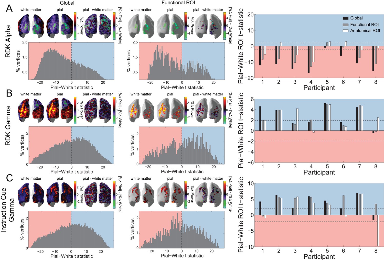
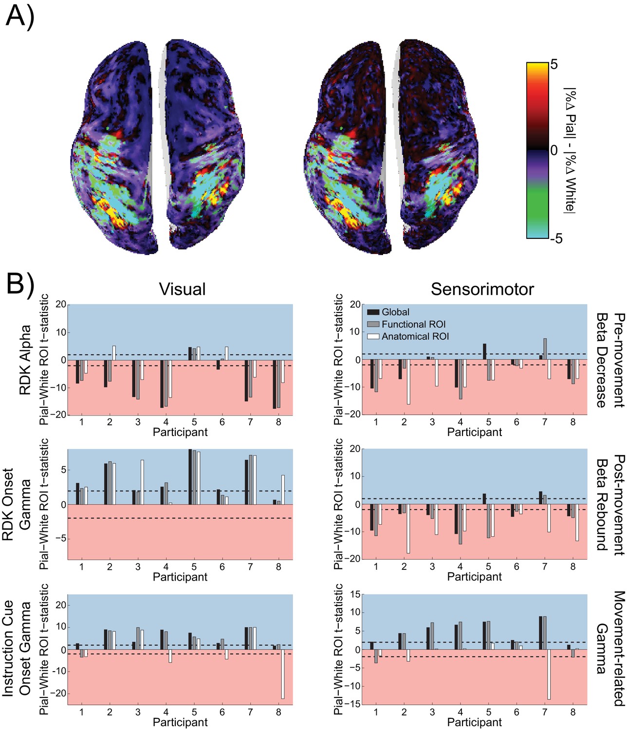
Laminar specificity of visual alpha and gamma.
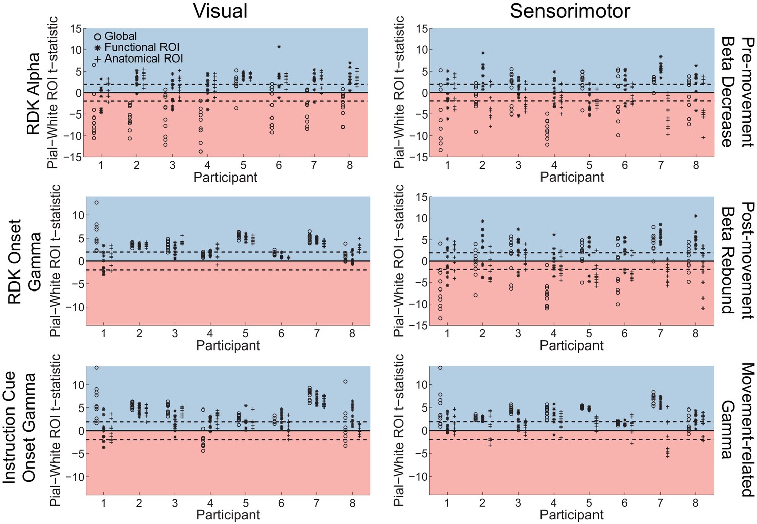
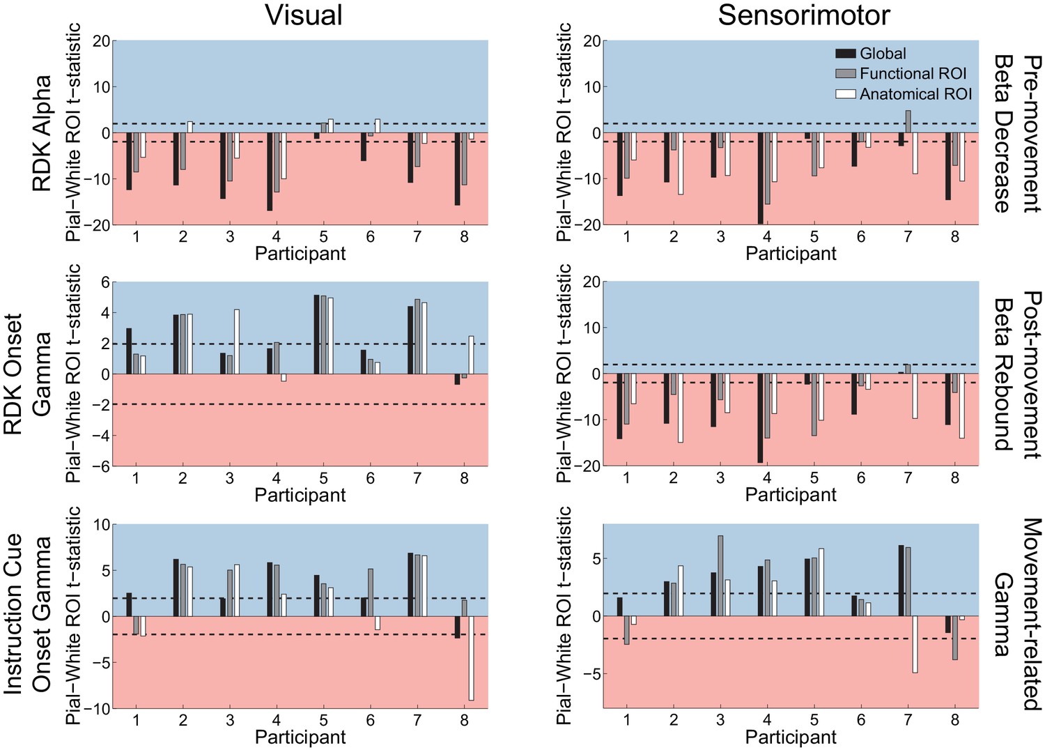
(A) Estimated changes in alpha power (7 – 13 Hz) from baseline on the white matter and pial surface, and the difference in the unsigned fractional change in power (pial – white matter) following the onset of the random dot kinematogram (RDK), over the whole brain (global) and within a functionally defined region of interest (ROI). Histograms show the distribution of t-statistics comparing the fractional change in power from baseline between corresponding pial and white matter surface vertices over the whole brain, or within the ROI. Negative t-statistics indicate a bias toward the white matter surface, and positive t-statistics indicate a pial bias. The bar plots show the t-statistics comparing the fractional change in power from baseline between the pial and white matter surfaces averaged within the ROIs, over all participants. T-statistics for the whole brain (black bars), functionally defined (grey bars), and anatomically constrained (white bars) ROIs are shown (red = biased toward the white matter surface, blue = biased pial). Dashed lines indicate the threshold for single participant statistical significance. (B) As in A, for gamma (60 – 90 Hz) power following the RDK. C) As in A and B, for gamma (60 – 90 Hz) power following the instruction cue. See Figure 5 – source data for raw data.
-
Figure 5—source data 1
Laminar comparison data for visual alpha (RDK) and gamma (RDK and instruction cue).
- https://doi.org/10.7554/eLife.33977.026
Figure 5—figure supplement 1
Sensor shuffling biases visual and sensorimotor laminar specificity to the pial surface.
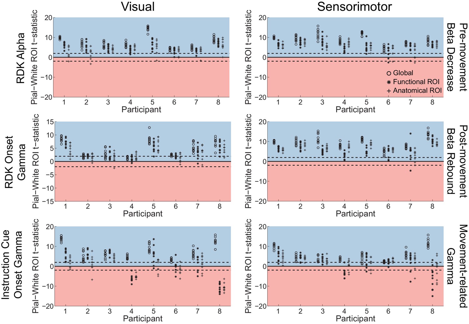
Each panel shows the t-statistics comparing the unsigned magnitude of the change in power between the pial and white matter surfaces, averaged within the regions of interests (ROIs), over all participants. T-statistics for the whole brain (circles), functionally defined (asterisks), and anatomically-constrained (crosses) ROIs are shown for 10 random sensor shuffles. Red background indicates a bias towards the white matter surface, and blue background a bias towards the pial surface. The dashed lines indicate single participant-level significance thresholds. Shuffling the sensor locations destroys the true mapping between the neural sources and the sensors, resulting in a bias toward the pial surface in all frequency bands and task epochs in both visual and sensorimotor cortex.
Figure 5—figure supplement 2
Adding coregistration error biases visual and sensorimotor laminar specificity to the pial surface.
Each panel shows the t-statistics comparing the unsigned magnitude of the change in power between the pial and white matter surfaces averaged within the regions of interests (ROIs), over all participants. T-statistics for the whole brain (circles), functionally defined (asterisks), and anatomically-constrained (crosses) ROIs are shown for 10 random fiducial coordinate perturbations involving a random translation (magnitude M = 10 mm, SD = 2.5 mm) and rotation (magnitude M = 10°, SD = 2.5°). These perturbations are within the range of commonly observed head movement with standard MEG recordings (Singh et al., 1997; Hillebrand and Barnes, 2011; Stolk et al., 2013; Troebinger et al., 2014b), but well above the head movement recorded in the present study. Red background indicates a bias towards the white matter surface, and blue background a bias towards the pial surface. The dashed lines indicate single participant-level significance thresholds.
Figure 5—figure supplement 3
Visual and sensorimotor laminar specificity compared to sensor shuffled data.
Each panel shows the t-statistics comparing the unsigned fractional change in power between the pial and white matter surfaces averaged within the regions of interests (ROIs), over all participants, testing against the null hypothesis that the difference between pial and white matter ROI values is given by the value obtained from sensor shuffling (rather than that they are equal). T-statistics for the whole brain (black bars), functionally defined (grey bars), and anatomically-constrained (white bars) ROIs are shown. Red background indicates a bias towards the white matter surface, and blue background a bias towards the pial surface. The dashed lines indicate single participant-level significance thresholds. As in the main laminar analysis, visual alpha activity localizes to the white matter surface (RDK alpha, global: W(8)=0.0, p=0.008, 7/8 participants; RDK alpha, functional ROI: W(8)=2, p=0.023, 6/8 participants; RDK alpha, anatomical ROI: W(8)=16, p=0.844, 4/8 participants), and visual gamma localizes to the pial surface (RDK gamma, global: W(8)=35, p=0.016, 4/8 participants; RDK gamma, functional ROI: W(8)=34, p=0.023, 4/8 participants; RDK gamma, anatomical ROI: W(8)=35, p=0.016, 5/8 participants; instruction cue gamma, global: W(8)=34, p=0.023, 6/8 participants; instruction cue gamma, functional ROI: W(8)=34, p=0.023, 6/8 participants; instruction cue gamma, anatomical ROI: W(8)=27, p=0.25, 5/8 participants). The results of sensorimotor beta and gamma mirrored these results, with beta localizing to the white matter surface (beta decrease, global: W(8)=0, p=0.008, 7/8 participants; beta decrease, functional ROI: W(8)=6, p=0.109, 7/8 participants; beta decrease, anatomical ROI: W(8)=0, p=0.008, 8/8 participants; beta rebound, global: W(8)=1, p=0.016, 7/8 participants; beta rebound, functional ROI: W(8)=1, p=0.016, 7/8 participants; beta rebound, anatomical ROI: W(8)=0, p=0.008, 8/8 participants), and localizing to the pial surface (global: W(8)=34, p=0.023, 5/8 participants; functional ROI: W(8)=33, p=0.039, 5/8 participants; anatomical ROI: W(8)=26, p=0.313, 4/8 participants).
Figure 5—figure supplement 4
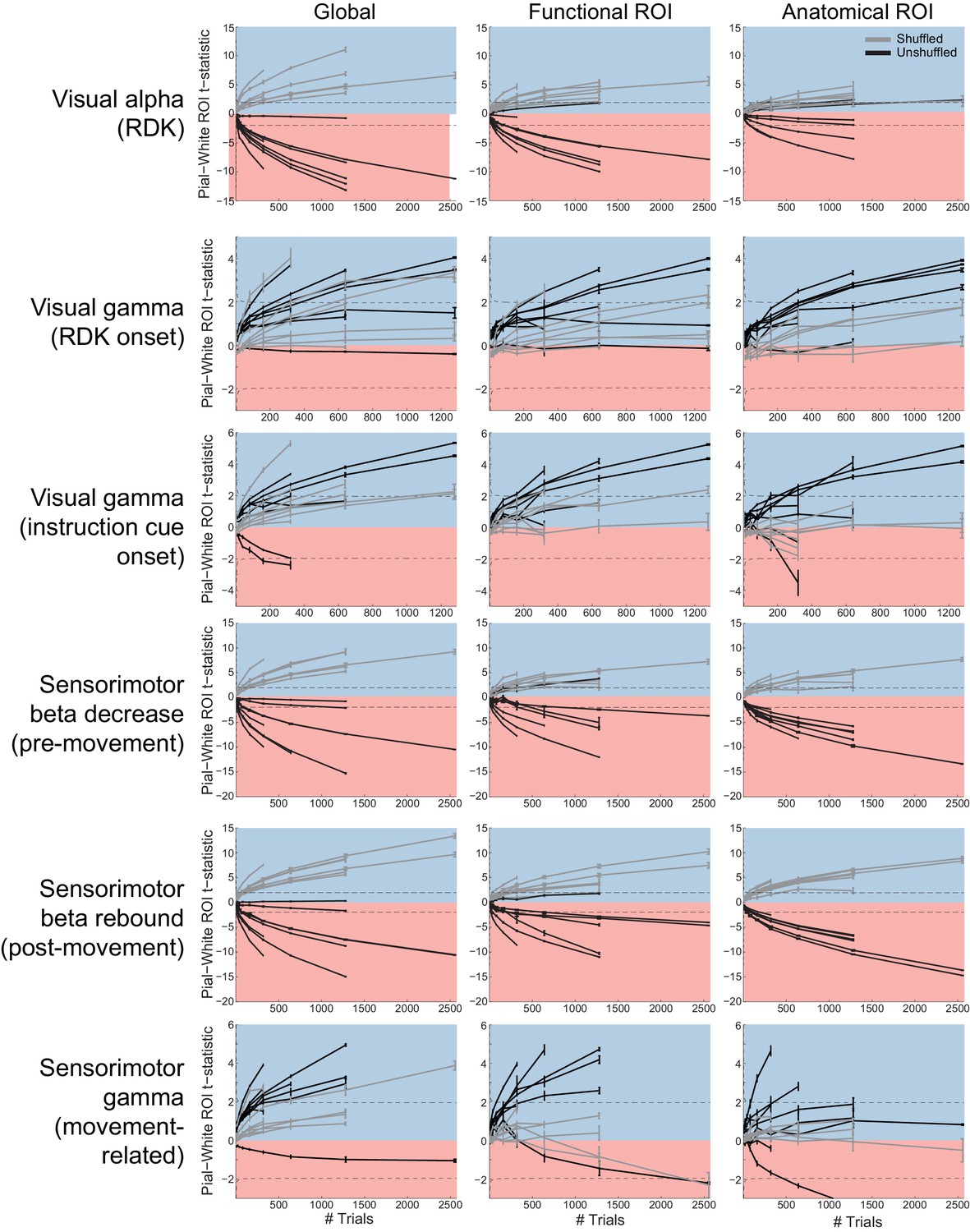
Laminar inference is a function of the number of trials.
Each panel shows the ROI t-statistics for (columns, left to right) the whole brain, functionally defined ROI, and anatomically constrained ROI, for each visual and sensorimotor signal (rows). Grey lines represent data with shuffled sensors, dark lines represent unshuffled data. Positive t-statistics (shaded blue) denote pial classification, and negative t-statistics (shaded red) denote white matter classification. The dashed lines indicate single participant-level significance thresholds. These data reveal that while laminar preference increases with the number of trials used in the analysis, this is as pronounced when the sensors are shuffled.
Figure 5—figure supplement 5
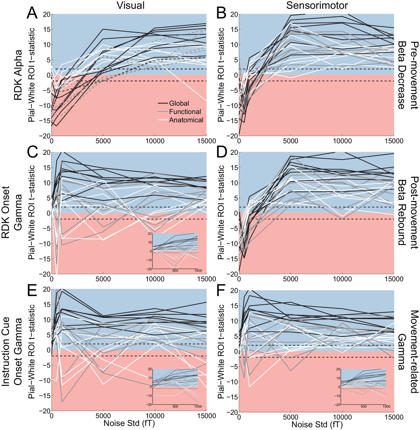
Laminar localization as a function of SNR.
Each panel shows the t-statistics for each participant, comparing the unsigned magnitude of the change in power from baseline between the pial and white matter surfaces. These statistics are shown for the global average (black lines), and for the functionally defined (grey lines) and anatomically constrained (white lines) ROIs, separately for each visual and sensorimotor signal. Different levels of white noise were added to the sensor level data, to reduce the SNR (standard deviation of white noise is on the x axis). The insets in panels C, E, and F show expanded versions of the full panel for gamma signals with added noise between 0 and 1000fT. The laminar localization of low- and high frequency signals is biased superficially overall after the introduction of sufficient levels of noise. The low-frequency signals become steadily more superficially biased before saturating as the level of noise increases, but the high frequency signals saturate at a much lower noise level and become unstable, flipping between superficial and deep for some subjects.
Figure 5—figure supplement 6
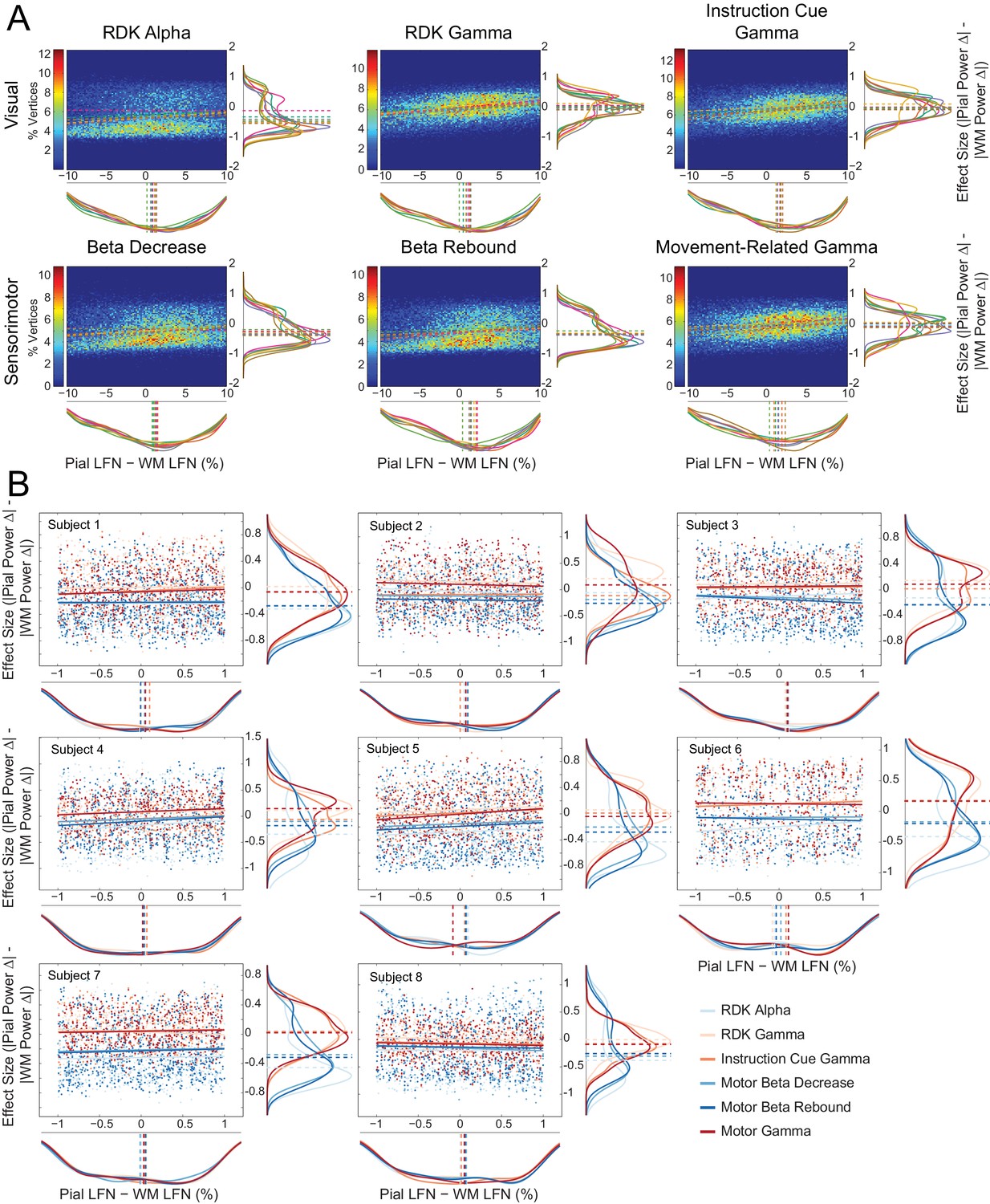
Laminar preference scales with the difference in pial and white matter lead field strength.
(A) Each panel shows normalized bivariate histograms of the difference in lead field strength (lead field norm, LFN, constrained within ±10% of the mean pial/white matter lead field norm) between corresponding vertices on the pial and white matter surfaces, plotted against the effect size (Cohen’s d) of the laminar bias. The laminar bias is defined as the unsigned fractional change in power from baseline on the pial surface, minus the unsigned fractional change in power on the white matter surface. The color of each pixel represents the percentage of vertices in the ROI that fall within that bin. The histograms are normalized to show the mean percentage of vertices in each bin over all participants. The fitted relationship between the lead field strength difference and laminar bias for each participant is shown as a dashed line. Kernel density estimates of the marginal distributions are shown below and to the right of each histogram, with each participant plotted in a different color. The median value for each participant is plotted as a vertical dashed line. There is a positive correlation between the difference in lead field strength between pial and white matter vertex pairs and laminar preference, with localization favoring the vertex with the strongest lead field (visual alpha (RDK): ρ = 0.14, t(7)=4.28, p<0.005; visual gamma (RDK): ρ = 0.30, t(7)=10.23, p<0.001; visual gamma (instruction cue): ρ = 0.29, t(7)=6.43, p<0.001; sensorimotor beta decrease: ρ = 0.18, t(7)=4.33, p<0.005; sensorimotor beta rebound: ρ = 0.20, t(7)=5.89, p<0.001; sensorimotor gamma: ρ = 0.25, t(7)=4.72, p<0.005). (B) Each panel shows, for a single participant over all comparisons, scatter plots and fitted linear relationships of the difference in lead field strength (lead field norm, LFN) between corresponding vertices on the pial and white matter surfaces (as a percentage of the average pial/white matter LFN, restricted to ±1%) plotted against the effect size (Cohen’s d) of the unsigned fractional change in power from baseline on the pial surface, minus the unsigned fractional change in power on the white matter surface. Kernel density estimates of the marginal distributions are shown below and to the right of each histogram, with low frequency signals plotted in blue and high frequency signals in red. The median value for each comparison is plotted as a vertical dashed line. Even when the pial and white matter vertices have approximately the same lead field strength, there is a clear laminar separation between low and high frequency signals, with low frequency signals localizing to the white matter surface (visual alpha (RDK): W(8)=0, p=0.008; sensorimotor beta decrease: W(8)=0, p=0.008; sensorimotor beta rebound: W(8)=0, p=0.008) and high frequency signals unbiased toward either surface with the exception of RDK visual gamma which is biased toward the pial surface (visual gamma (RDK): W(8)=36, p=0.008; visual gamma (instruction cue): W(8)=16, p=0.844; sensorimotor gamma: W(8)=26, p=0.313).
Figure 5—figure supplement 7

The relationship between pial and white matter lead field strength and laminar preference is the same across frequency bands.
Each panel shows the fitted linear relationship between the difference in lead field strength between the pial and white matter surfaces (pial lead field norm – white matter lead field norm), and the effect size (Cohen’s d) of the unsigned fractional change in power from baseline on the pial surface, minus the unsigned fractional change in power on the white matter surface. The panels show this relationship for pairs of corresponding pial/white matter vertices over the whole range of lead field norm differences (A) and within ±10% of the average pial/white matter lead field norm difference (B) over all participants. There is no significant effect of frequency band or region on the correlation between lead field norm difference and laminar preference.
Figure 5—figure supplement 8
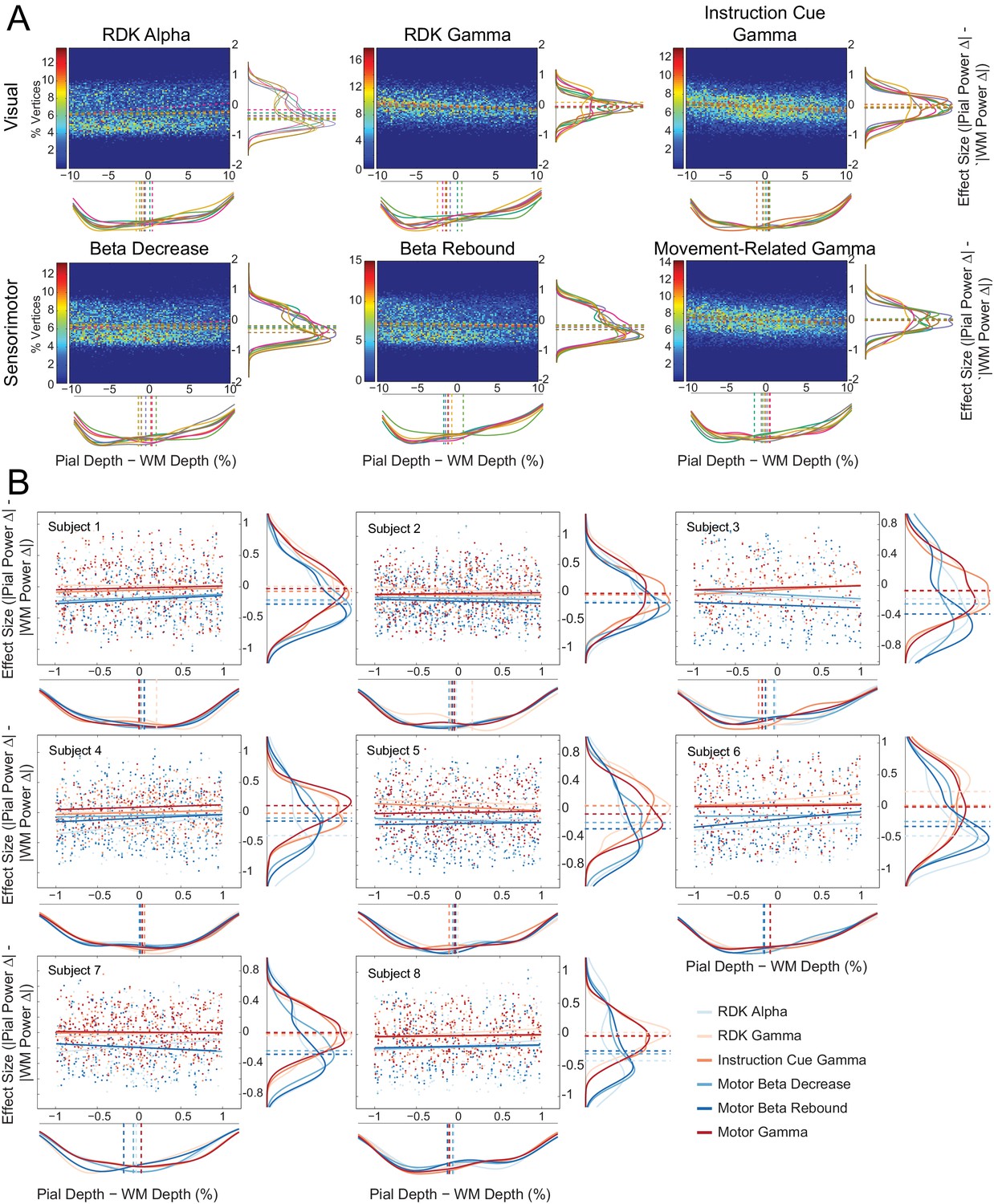
Laminar preference does not relate to the difference in vertex depth.
(A) As in Figure 5—figure supplement 6A, but with the difference in depth between corresponding vertices on the pial and white matter surfaces (constrained within ±10% of the mean pial/white matter depth) along the x axis of each plot. There is no correlation between the relative distance to the scalp between pial and white matter vertex pairs and laminar preference (visual alpha (RDK): ρ = 0.05, t(7)=2.15, p=0.068; visual gamma (RDK): ρ = −0.10, t(7)=-7.08, p<0.001; visual gamma (instruction cue): ρ = −0.02, t(7)=-0.90, p=0.398; sensorimotor beta decrease: ρ = 0.02, t(7)=0.58, p=0.581; sensorimotor beta rebound: ρ = −0.02, t(7)=-1.09, p=0.311; sensorimotor gamma: ρ = −0.04, t(7)=-1.02, p=0.341). (B) As in Figure 5—figure supplement 6B, but with the difference in depth between the surfaces (pial – white matter) along the x axis of each plot. Even when the pial and white matter vertices are at approximately the same distance to the scalp, there is a clear laminar separation between low and high frequency signals, with low frequency signals localizing to the white matter surface (visual alpha (RDK): W(8)=0, p=0.008; sensorimotor beta decrease: W(8)=0, p=0.008; sensorimotor beta rebound: W(8)=0, p=0.008) and high frequency signals unbiased toward either surface (visual gamma (RDK): W(8)=29, p=0.148; visual gamma (instruction cue): W(8)=11, p=0.383; sensorimotor gamma: W(8)=11, p=0.383).
Figure 5—figure supplement 9
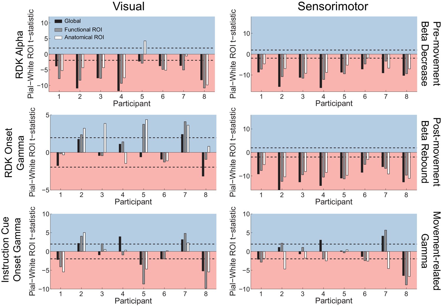
Laminar localization does not reverse for vertex pairs in which the white matter surface is closer to the scalp than the pial surface.
Each panel shows the t-statistics comparing the unsigned fractional change in power from baseline between the pial and white matter surfaces for each participant. Only pairs of corresponding white matter and pial surface vertices were included in which the white matter vertex was closer to the scalp surface than the pial vertex. T-statistics for the whole brain (black bars), functionally defined (grey bars), and anatomically constrained (white bars) ROIs are shown (red background = biased toward the white matter surface, blue background = biased pial). Dashed lines indicate the threshold for single participant statistical significance. Even considering only patches of cortex where the white matter surface was closer to the scalp than the pial surface, the gamma localization did not reverse to the white matter surface. Visual alpha still localized predominantly to the white matter surface (global: W(8)=0, p=0.008, 8/8 participants white matter; functional ROI: W(8)=0, p=0.008, 8/8 participants white matter; anatomical ROI: W(8)=1, p=0.016, 6/8 participants white matter, 1/8 pial, 1/8 no bias). For RDK- and instruction cue-locked gamma, the laminar preference was overall weaker (RDK gamma, global: W(8)=19, p=0.945, 1/8 participants pial, 1/8 white matter, 6/8 no bias; RDK gamma, functional ROI: W(8)=25, p=0.383, 3/8 participants pial, 5/8 no bias; RDK gamma, anatomical ROI: W(8)=28, p=0.195, 4/8 participants pial, 4/8 no bias; instruction cue gamma, global: W(8)=19, p=0.945, 3/8 participants pial, 4/8 white matter, 1/8 no bias; instruction cue gamma, functional ROI: W(8)=21, p=0.742, 3/8 participants pial, 4/8 white matter, 1/8 no bias; instruction cue gamma, anatomical ROI: W(8)=21, p=0.742, 2/8 participants pial, 3/8 white matter, 3/8 no bias). Sensorimotor beta still localized to the white matter surface (beta decrease, global: W(8)=0, p=0.008, 8/8 participants white matter; beta decrease, functional ROI: W(8)=0, p=0.008, 8/8 participants white matter; beta decrease, anatomical ROI: W(8)=0, p=0.008, 7/8 participants white matter, 1/8 no bias; beta rebound, global: W(8)=0, p=0.008, 8/8 participants white matter; beta rebound, functional ROI: W(8)=0, p=0.008, 8/8 participants white matter; beta rebound, anatomical ROI: W(8)=0, p=0.008, 8/8 participants white matter). In this case, sensorimotor gamma did not reliably localize to either surface at the group level globally or in the functional ROI (global: W(8)=20, p=0.844, 2/8 participants pial, 2/8 white matter, 4/8 no bias; functional ROI: W(8)=15, p=0.742, 2/8 participants pial, 4/8 participants white matter, 2/8 no bias), and was biased more towards the white matter surface in the anatomical ROI for these selected vertices (W(8)=1, p=0.016, 5/8 participants white matter, 3/8 no bias).
Figure 5—figure supplement 10
Visual and sensorimotor laminar specificity does not change after controlling for distance to the scalp.
(A) An example global map of difference in the unsigned fractional change in power from baseline between the pial and white matter surfaces during the sensorimotor beta decrease, shown for a representative participant before (left) and after (right) controlling for the influence of the distance between each vertex and the scalp. (B) Each panel shows the t-statistics comparing the residual error of a linear regression relating the square root of the mean distance to scalp (averaged over pial – white matter vertex pairs) to the difference in the unsigned fractional change in power from baseline between the pial and white matter surfaces for each participant. T-statistics for the whole brain (black bars), functionally defined (grey bars), and anatomically constrained (white bars) ROIs are shown (red background = biased toward the white matter surface, blue background = biased pial). Dashed lines indicate the threshold for single participant statistical significance. After controlling for the effect of depth, visual alpha still localized predominantly to the white matter surface (global: W(8)=1, p=0.016, 7/8 participants white matter, 1/8 pial; functional ROI: W(8)=4, p=0.055, 6/8 participants white matter, 1/8 pial, 1/8 no bias; anatomical ROI: W(8)=15, p=0.742, 5/8 participants white matter, 3/8 pial). For RDK- and instruction cue-locked gamma, the laminar preference was still biased toward the pial surface (RDK gamma, global: W(8)=36, p=0.008, 7/8 participants pial, 1/8 no bias; RDK gamma, functional ROI: W(8)=36, p=0.014, 4/8 participants pial, 4/8 no bias; RDK gamma, anatomical ROI: W(8)=36, p=0.008, 6/8 participants pial, 2/8 no bias; instruction cue gamma, global: W(8)=36, p=0.008, 8/8 participants pial; instruction cue gamma, functional ROI: W(8)=34, p=0.023, 7/8 participants pial, 1/8 white matter; instruction cue gamma, anatomical ROI: W(8)=26, p=0.313, 4/8 participants pial, 4/8 white matter). Sensorimotor beta still localized to the white matter surface (beta decrease, global: W(8)=9, p=0.25, 5/8 participants white matter, 1/8 pial, 2/8 no bias; beta decrease, functional ROI: W(8)=8, p=0.195, 6/8 participants white matter, 1/8 pial, 1/8 no bias; beta decrease, anatomical ROI: W(8)=0, p=0.008, 8/8 participants white matter; beta rebound, global: W(8)=11, p=0.383, 6/8 participants white matter, 2/8 pial; beta rebound, functional ROI: W(8)=4, p=0.055, 7/8 participants white matter, 1/8 pial; beta rebound, anatomical ROI: W(8)=0, p=0.008, 8/8 participants white matter), and sensorimotor gamma still localized to the pial surface (global: W(8)=36, p=0.008, 7/8 participants pial, 1/8 no bias; functional ROI: W(8)=33, p=0.039, 6/8 participants pial, 2/8 white matter; anatomical ROI: W(8)=17, p=0.945, 2/8 white matter, 6/8 no bias).
Figure 5—figure supplement 11
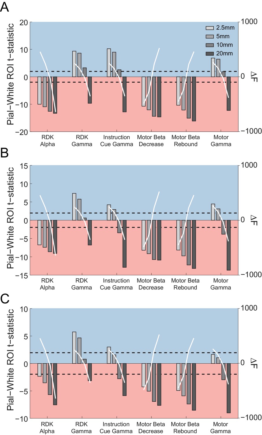
The relationship between patch size estimates and laminar bias.
Each panel shows the t-statistics for a representative participant comparing the unsigned fractional change in power from baseline between the pial and white matter surfaces averaged globally (A) and within the functionally defined (B) or anatomically constrained (C) ROIs for each visual and sensorimotor signal, and four different patch sizes (2.5, 5, 10, and 20 mm). The difference in free energy from the mean (ΔF) for inversions performed within each frequency band on the combined pial/white matter surface for each patch size is shown by the overlaid white lines. Increasing patch sizes bias the localization toward deep sources, but at the optimal patch sizes (largest free energy difference), low frequency signals localize to the deep laminae and high frequency signals localize superficially.
Figure 5—figure supplement 12
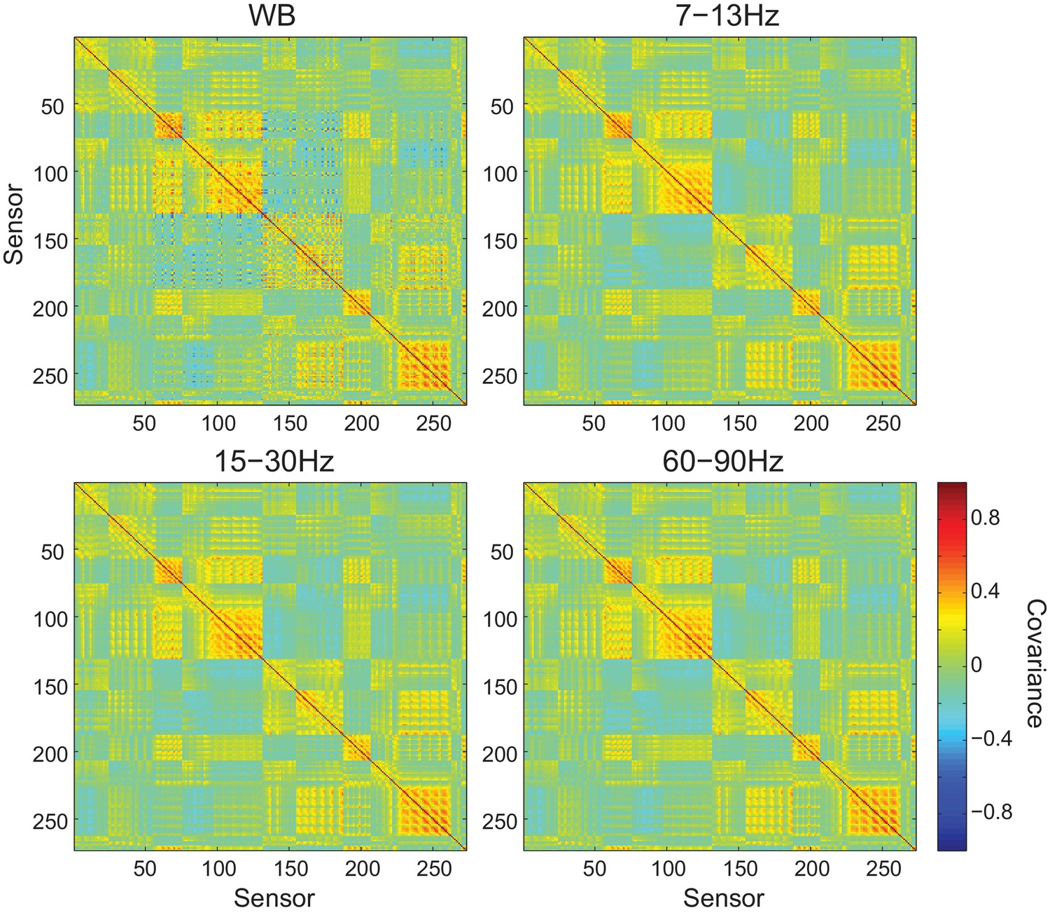
Sensor covariance is similar across frequency bands.
Each panel shows the sensor covariance computed from empty room recordings for wide band (WB) and filtered data within each frequency band analyzed. While the covariance matrices are not perfectly diagonal, they are similar across frequency bands.
Figure 5—figure supplement 13
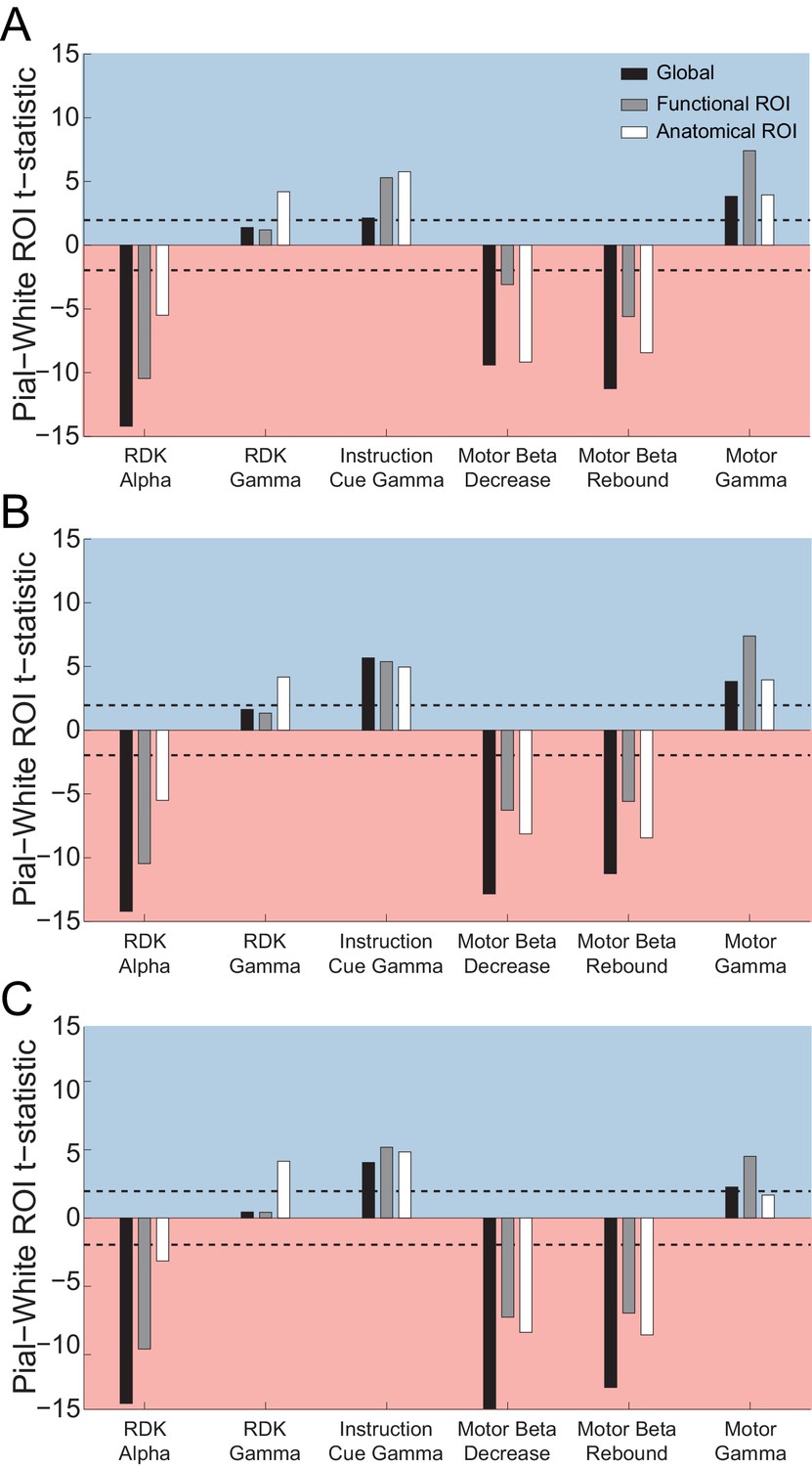
Laminar localization is not affected by regularization or sensor covariance.
Each panel shows the t-statistics for a representative participant comparing the unsigned magnitude of the change in power from baseline between the pial and white matter surfaces averaged globally (black bars), and within the functionally defined (grey bars) or anatomically constrained (white bars) ROIs for each visual and sensorimotor signal. The laminar localization of each signal in each ROI is the same using EBB source inversion without regularization and assuming uncorrelated sensor noise (A), with (B) source priors at multiple levels of regularization, and (C) using an empirical (Figure 5—figure supplement 12) sensor covariance matrix.
Figure 6
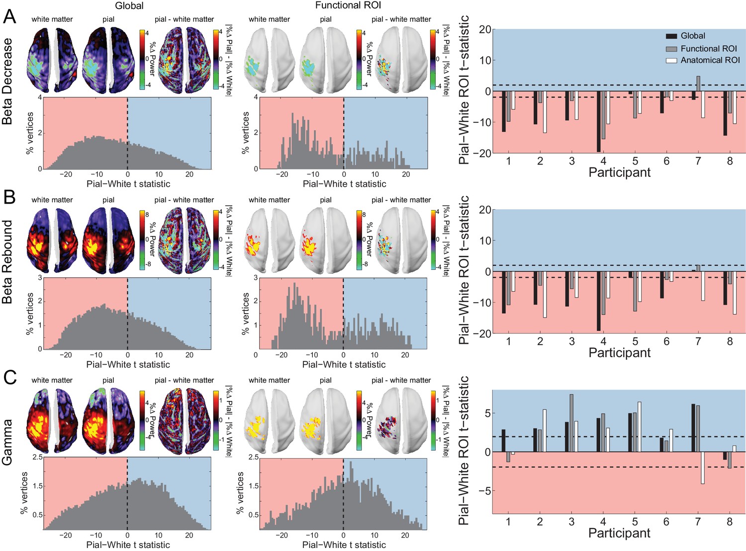
Laminar specificity of sensorimotor beta and gamma.
As in Figure 5, for (A) the beta (15 – 30 Hz) decrease prior to the response, (B) beta (15 – 30 Hz) rebound following the response, and (C) gamma (60 – 90 Hz) power change from baseline during the response. In the histograms and bar plots, positive and negative values indicate a bias towards the superficial and deeper cortical laminae, respectively. The dashed lines indicate single participant-level significance thresholds. The black, grey, and white bars indicate statistics based on regions of interest comprising the whole brain, functional and anatomically-constrained ROIs, respectively. See Figure 6 – source data for raw data.
-
Figure 6—source data 1
Laminar comparison data for sensorimotor beta decrease, beta rebound, and gamma.
- https://doi.org/10.7554/eLife.33977.028
Figure 7
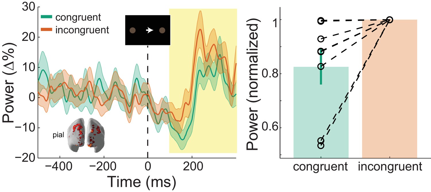
: Visual gamma activity modulation by task condition.
Visual gamma activity following the onset of the instruction stimulus within the functionally defined ROI of an example participant (left), and averaged within the time window represented by the shaded yellow rectangle for all participants (right). Each dashed line on the right shows the change in normalized values for the different conditions for each participant. The bar height represents the mean normalized change in gamma power, and the error bars denote the standard error. Visual gamma activity is stronger following the onset of the instruction cue when it is incongruent to the direction of the coherent motion in the random dot kinematogram (RDK). See Figure 7 – source data for raw data.
-
Figure 7—source data 1
Condition comparison data for visual gamma (instruction cue).
- https://doi.org/10.7554/eLife.33977.030
Figure 8
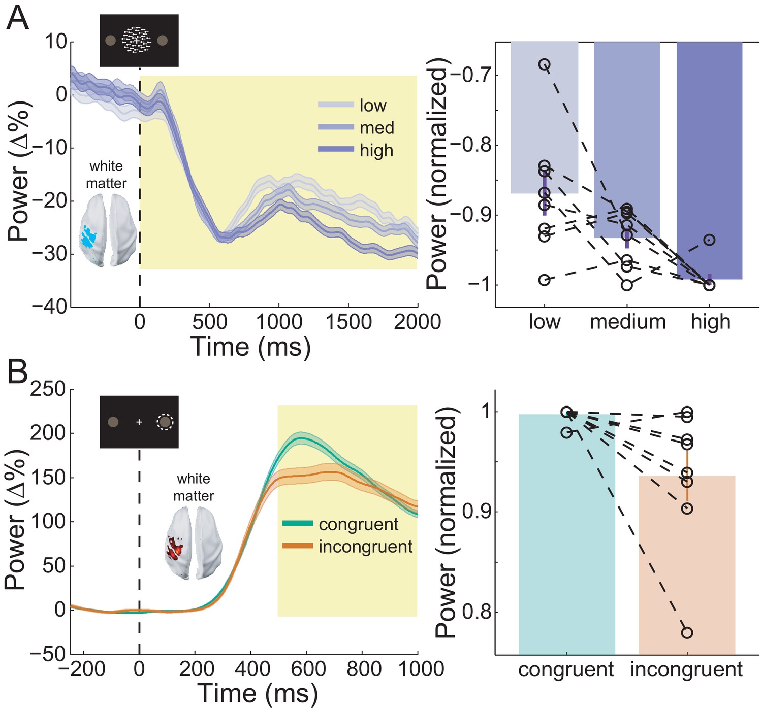
Sensorimotor beta activity modulated by task condition.
(A) Beta decrease following the onset of the random dot kinematogram (RDK) within the functionally defined ROI of an example participant over the duration of the RDK (left), and averaged over this duration for all participants (right). The bar height represents the mean normalized change in beta power, and the error bars denote the standard error. The beta decrease becomes more pronounced with increasing coherence. (B) As in A, for beta rebound following the response and averaged within the time window shown by the shaded yellow rectangle. Beta rebound is stronger following responses in congruent trials. See Figure 8 – source data for raw data.
-
Figure 8—source data 1
Condition comparison data for sensorimotor beta decrease and beta rebound.
- https://doi.org/10.7554/eLife.33977.032
Author response image 1
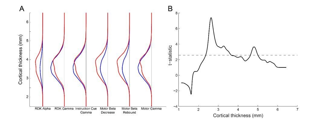
Laminar specificity across the range of cortical thickness.
(A) The y-axis represents the distance between the pial and white matter vertices (cortical thickness). For each visual and sensorimotor frequency band and task epoch (x axis), the probability density function for pial (blue line) and white matter (red line) classifications is shown over the range of cortical thickness. There is a bias toward the white matter surface where the cortex is thick (~4mm and thicker), and toward the pial surface here the cortex is thinner (~3.5mm). However, the overall pial/white matter bias is driven by the frequency band. (B) The y-axis represents the t-statistic from a one-way t-test of the difference in the probability density of cortical classification across each frequency band and task epoch (pial-white for gamma, and white-pial for alpha and beta). The ability to discriminate between laminae drops off when the cortical thickness is below 2.5mm.
Author response image 2
Additional files
-
Transparent reporting form
- https://doi.org/10.7554/eLife.33977.033
Download links
A two-part list of links to download the article, or parts of the article, in various formats.
Downloads (link to download the article as PDF)
Open citations (links to open the citations from this article in various online reference manager services)
Cite this article (links to download the citations from this article in formats compatible with various reference manager tools)
Lamina-specific cortical dynamics in human visual and sensorimotor cortices
eLife 7:e33977.
https://doi.org/10.7554/eLife.33977


