Transformation of temporal sequences in the zebra finch auditory system
- Boston University, United States
- Korea Institute of Science and Technology, Korea
Figures
Figure 1 with 3 supplements
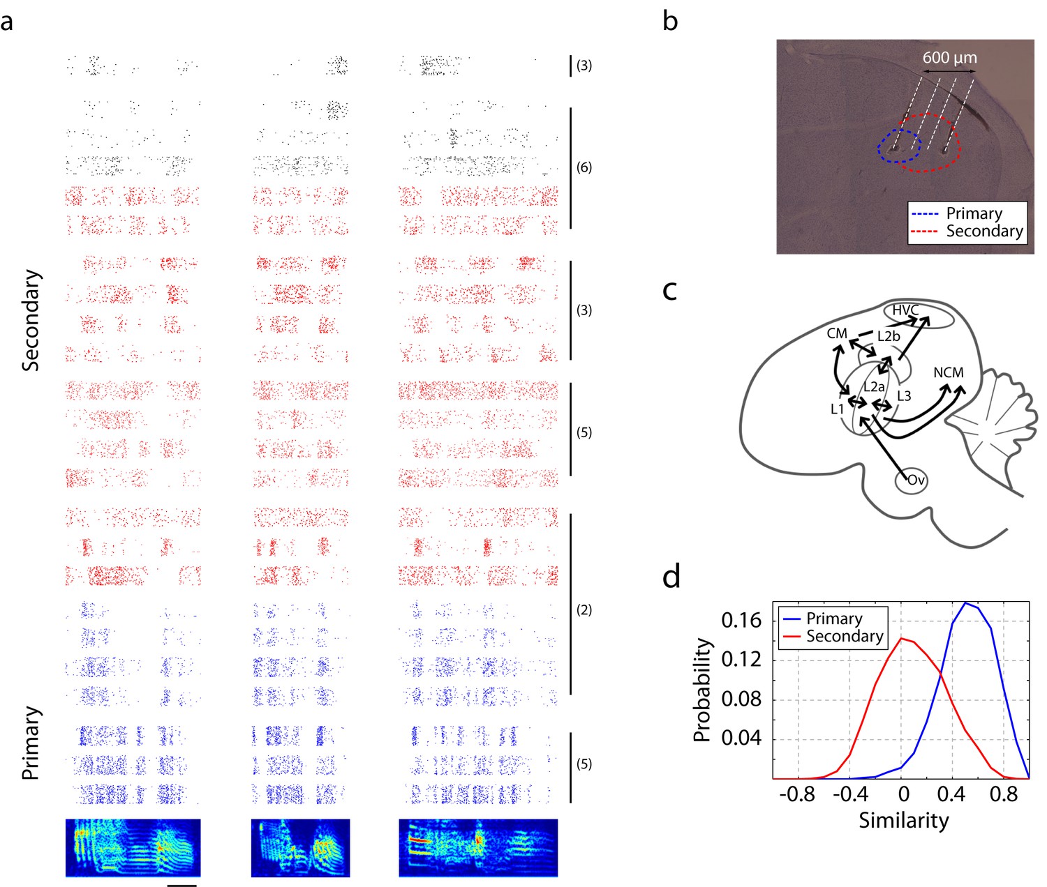
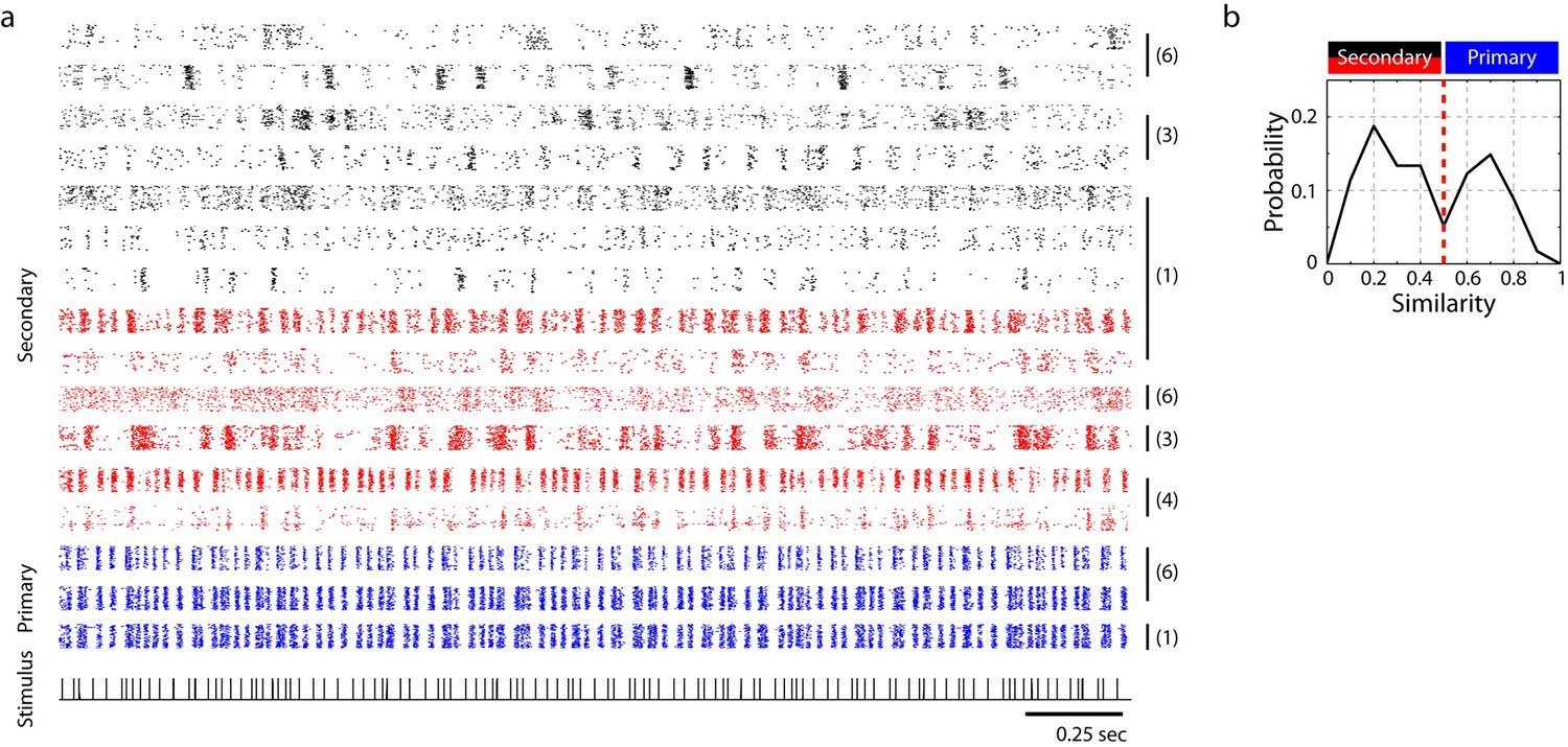
Neural responses in primary and secondary auditory areas to birdsongs.
(a) Example of neural responses in primary (blue) and secondary auditory areas (red and black) to birdsongs. Syllable responses were extracted from playback of whole songs. Individual cells in this figure were recorded in different birds. Numbers on the right correspond to the bird indices shown in Figure 1—figure supplement 1. Cells in the primary auditory area, L2a, respond more synchronously than cells in the secondary area. Red and black colors in the raster denote two classes of cells in secondary auditory areas defined by spike-width. (For red, spike width is less than 250 µs , and for black, greater than 250 µs.) The scale bar is 50 ms. (b) Sagittal section located at 1.5 mm lateral of the midline with estimated electrode shank positions (dotted white line). Physiological locations are confirmed by the anatomy (Figure 1—figure supplement 1). (c) Schematic of a sagittal section of male zebra finch brain. (d) Response similarity scores between all pairs of cells in the secondary auditory area are lower than similarity scores in the primary auditory area. (Secondary auditory responses to song are more diverse across neurons.)
Figure 1—figure supplement 1
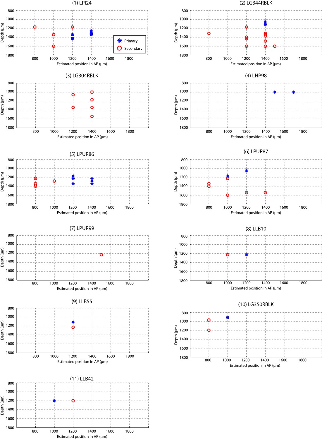
Estimated recording location of units.
Cells were colored by their classification as primary or secondary cells based on response latency and similarity scores (Figures 1d and 3b). This figure shows that for each bird, the primary and secondary cells were spatially separable, providing independent confirmation that the classification as primary and secondary cortical neurons was accurate. On each graph, estimated spatial positions of primary (blue star) and secondary (red circles) units are shown. Positions were approximated based on the configuration of electrode and recording coordinates.
Figure 1—figure supplement 2
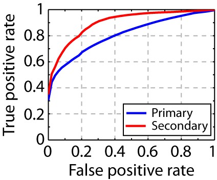
Song syllable discriminability analysis.
ROC analysis shows increased discriminability of song syllables in secondary auditory areas, L2b and L3, relative to primary auditory area, L2a (n = 13 syllables).
Figure 1—figure supplement 3
Peri-stimulus time histogram (PSTH) of song responses.
The PSTH of neurons in primary auditory area, L2a, reveal synchronous responses to song (bin size: 5 ms). In this figure, the average PSTH of all neurons is shown.
Figure 2
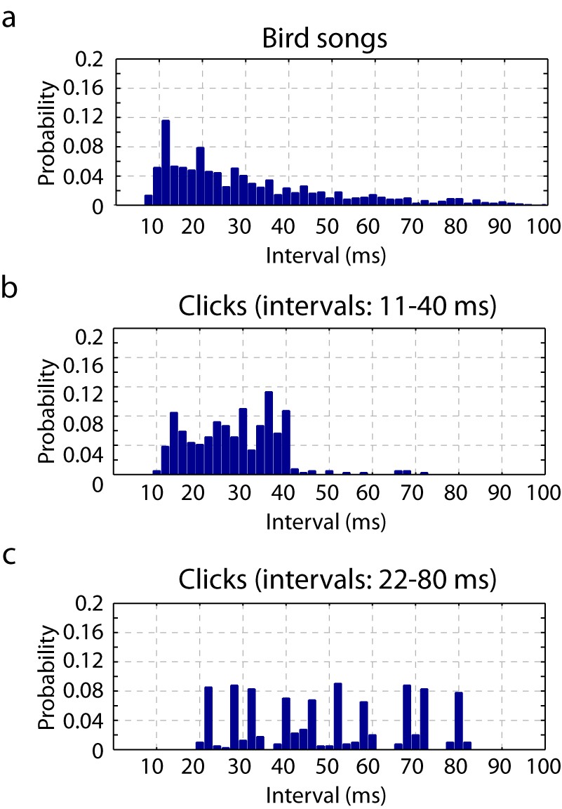
Timescales of neural responses in the primary auditory area, L2a.
(a) Interval histogram of peaks in the PSTH of neurons in the primary auditory area, L2a, in response to bird songs. The population PSTH contains intervals distributed from 10 ms to 40 ms. (b,c) Interval histogram of peaks in the PSTH of neurons in the primary auditory area, L2a, in response to click sequences. For the click patterns, we applied two different timescales for the click intervals. In the first timescale, the click sequence evokes PSTH intervals in the range of 10–40 ms. The slower set of stimuli evokes PSTH intervals in the range of 20–80 ms.
Figure 3 with 5 supplements
Neural responses to click sequences in primary and secondary auditory areas.
(a) Example of neural responses in primary and secondary auditory areas. Units from individual birds are grouped (black vertical bars and corresponding bird indices are shown on the right of the rasters). Red and black rasters mark two classes of cells in secondary auditory areas that are defined by spike-width. For red rasters, the spike width is less than 250 µs and for black, greater than 250 µs). Blue rasters are cells in the primary auditory area, L2a. (b) Histogram of cross-correlation scores between the click stimulus and the PSTH response. The discrimination line between two peaks (at 0.5 similarity score) also segregates the cells spatially (Figure 1—figure supplement 1), confirming the classification of neurons as residing in spatially separated areas – either L2a or L3/L2b.
Figure 3—figure supplement 1
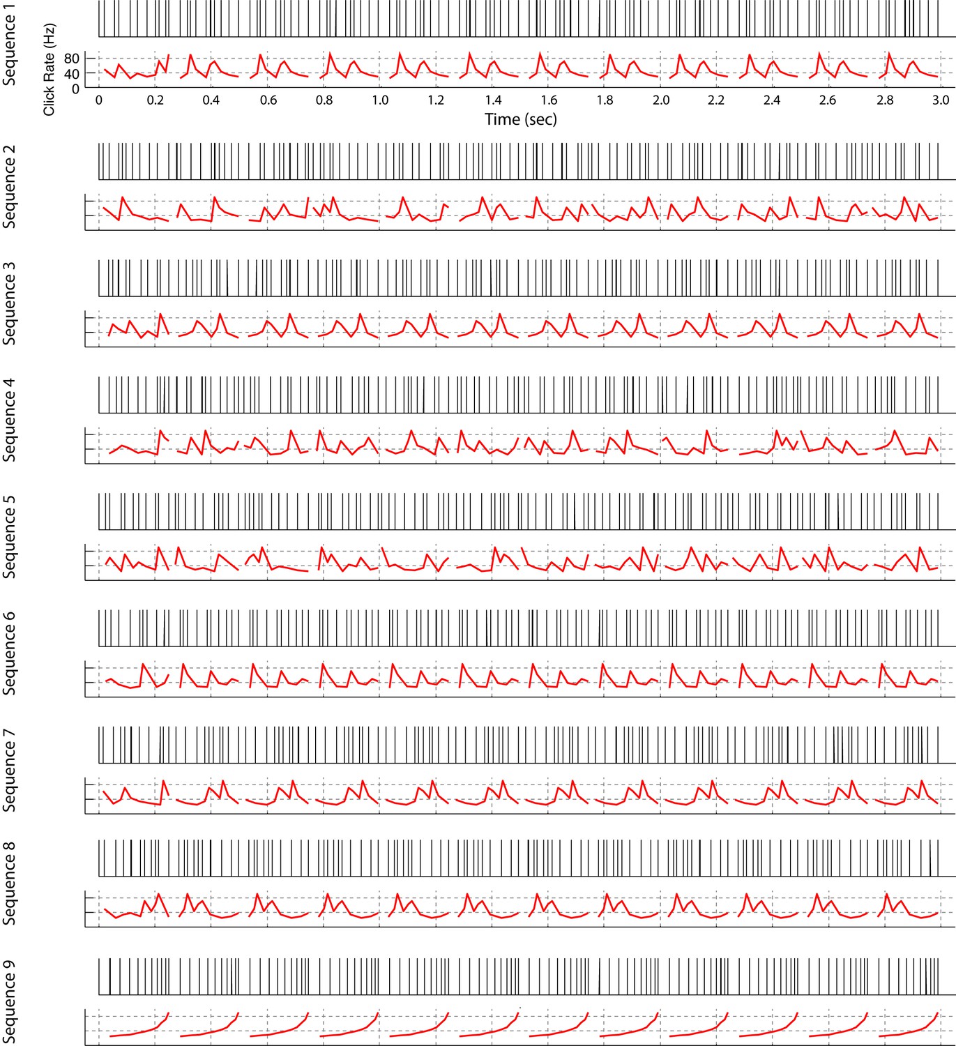
All click sequences used for neural recordings and operant training.
Click sequences were repeating or non-repeating temporal patterns. Each temporal pattern is 249 ms long and the total length of the sequence is 3 s. For sequences 1, 3, 6, 7, 8, and 9, a single fixed temporal pattern repeats 11 times; the other sequences are composed of 11 different non-repeating patterns. We also built some sequences in reverse order (Seq. 1 vs Seq. 3, Seq. 2 vs Seq. 4, Seq. 7 vs Seq. 8). Sequences 1–8 were used for neural recording and sequences 1, 2, and 9 were used for the operant-training experiment. An audio file for each click sequence is provided (Supplementary file 1).
Figure 3—figure supplement 2
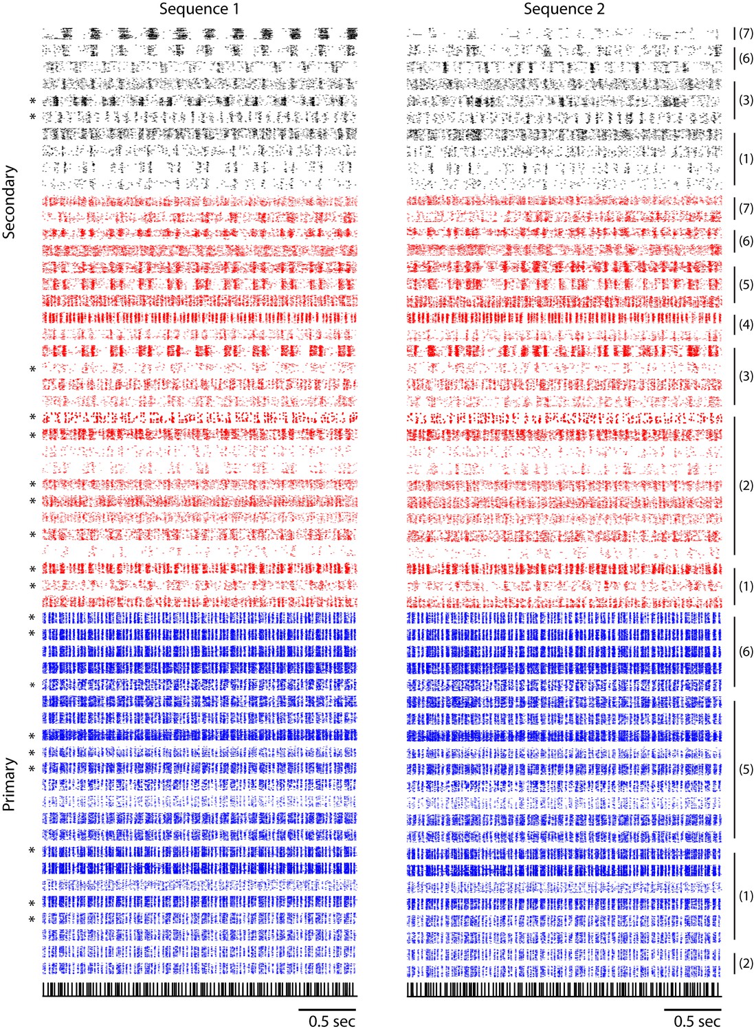
Combined single and multi-unit responses to sequence 1 and sequence 2.
Responses in the primary auditory area, L2a, are shown in blue and those in secondary areas, L2b/L3, are shown in red and black. Multi-unit responses, as opposed to single-unit responses, are indicated by asterisk marks on the left. Responses from a single bird are grouped by a black vertical bar, with the corresponding bird index on the right. Two different classes of neurons in the secondary auditory areas (red and black rasters) are classified based on the peak-to-peak width of spike waveform following the conventions of Figure 3a.
Figure 3—figure supplement 3

Example spike waveforms corresponding to click responses shown in raster form.
Each row of the raster plot represents the single-unit responses to a click sequence (sequence 2); the corresponding spike waveform is shown on the right. The shaded error bars represent the standard deviation of waveforms. Primary L2a neurons are shown in blue. Narrow- and broad-spiking units in L2b or L3 are shown in red and black, respectively.
Figure 3—figure supplement 4
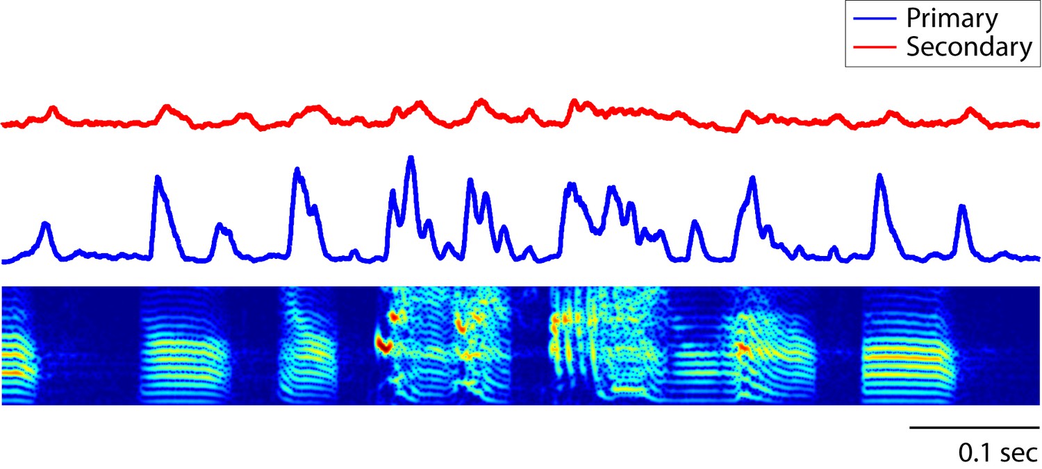
Population PSTH of neurons in response to click sequences.
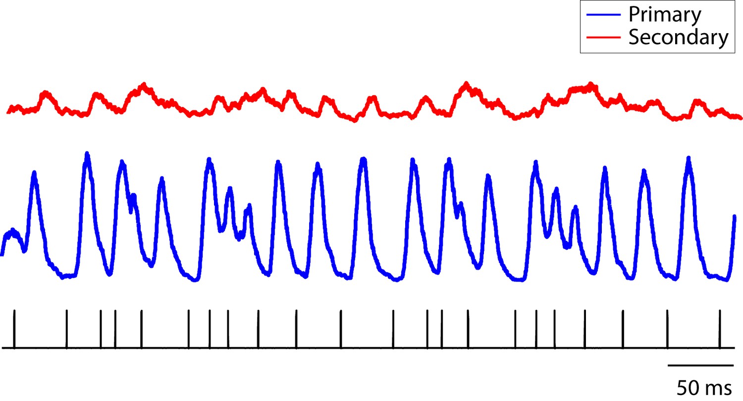
The combined population PSTH of neurons in the primary auditory area, L2a, is deeply modulated, a result of synchronous responses to the click sequence (blue trace, bin size: 5 ms). The combined population PSTH of neurons in secondary areas (L2b and L3) is shown in red. The bottom tick marks show the waveform of the click stimulus (click sequence 1).
Figure 3—figure supplement 5
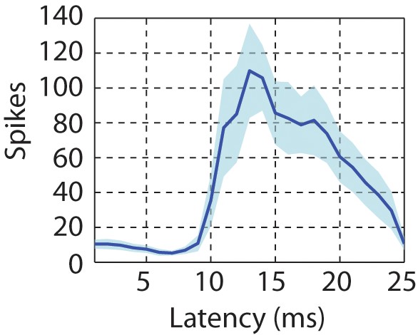
Latency of neural responses to click sequences in the primary auditory area, L2a.
To calculate the latency in the primary auditory area, a click-triggered histogram of single-unit responses is generated. The origin of this plot corresponds to the onset time of each click. The solid line represents the mean latency histogram and the shaded error bar is standard deviation of latency.
Figure 4 with 1 supplement

Temporal sequences are transformed to distinct population vectors in the secondary auditory areas, L2b and L3.
(a) For different stimuli, ensemble state-space trajectories are discriminable in secondary auditory areas but not in the primary auditory area, L2a. For each trace, the bin size for the ensemble state space was 5 ms. Each trace is smoothed by rectangular windows (10 ms) for visualization. (b) Receiver operating characteristic (ROC) analysis reveals enhanced discriminability of click sequences in secondary auditory areas, L2b and L3, relative to those in the primary auditory area, L2a.
-
Figure 4—source data 1
Source data for ROC curve.
This zip file contains spike-timing data used for the ROC analysis shown in Figure 4b. Spike times of 10 different cells recorded in primary or secondary auditory areas are included in folders with corresponding names. For simple visualization of spike rasters, Matlab source code (DataLoad.m) is also provided.
- https://doi.org/10.7554/eLife.18205.014
Figure 4—figure supplement 1
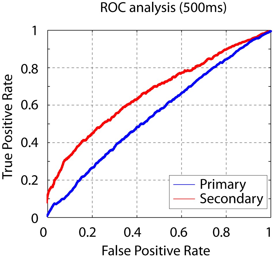
Short click-sequence discriminability analysis.
ROC analysis shows that the sequence discriminability in secondary auditory areas is maintained even when considering only the first 500 ms of the neural response.
Figure 5 with 1 supplement

Neural sequence discriminability depends on the timescale of the click sequence.
ROC analysis reveals that the discriminability of the click sequences is constrained by the interval distribution of the click stimuli. When the sequence is slowed by a factor of two, the discriminability of click sequences is lost in the secondary auditory area (shown in green).
Figure 5—figure supplement 1
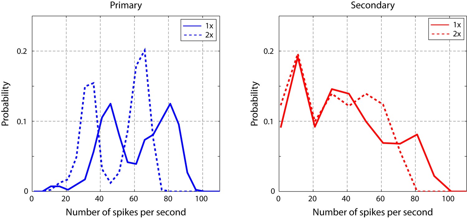
Spike rate of cells in response to click sequences with different timescales.
Slower click sequences evoke a lower spike rate in primary and secondary auditory areas. For the secondary auditory areas, this reduction in spike rate is relatively small. This analysis was based on data used in Figure 5.
Figure 6 with 2 supplements

Operant training with click sequences.
(a) Example of training by the single-stage behavioral-shaping method. The probability distribution of accessing trial port and water port is illustrated on a log scale. The white dotted line represents the start of sequence playback and the white solid line is the termination time of the stimulus. We show two stimuli back to back with mirrored time axes. Asymmetry between the solid lines in this image indicates learning. Over the course of training, this bird started to interrupt playback of the non-rewarding sequence by accessing the trial port before sequence 1 (the unrewarded sequence) stopped playing. The bird also learned to access the water port selectively during the playback of the rewarded sequence (sequence 2). (b) Learning curve for birds exposed to the single-stage training method (n = 8 birds). With the single-stage training method, most birds start to show differentiated responses (d’ is around 1) after two weeks of training; that is, they interrupt and reset sequence 1 playback and access the water port for sequence 2 playback. (c) When the click intervals are slowed by a factor of two, all trained birds (n = 11 in the single-stage method) were unable to discriminate the temporal sequences; d’ is around 0.
-
Figure 6—source data 1
Summary of training.
The success of operant training was determined on the basis of the d-prime score. When d’ is greater than 1, the bird was deemed successful in learning the task. In this table, the number of birds that succeeded in operant training for click sequence discrimination (d’ > 1) out of the total number of birds is shown. For example, 8 out of 10 birds succeeded in two-stage training to discriminate sequence 9 and 2.
- https://doi.org/10.7554/eLife.18205.019
Figure 6—figure supplement 1

Operant training setup.
There are two infrared switches, a green LED (trial indicator) and a water spout in the training cage. An Arudino microprocessor monitors the timing of port access, plays stimuli, and delivers water rewards. The water reservoir is located 24 inches above the floor of cage. The water valve is opened for a fixed duration, just long enough to produce a drop of water that is consistently 1–5 μl in volume. During operant training, data collected by the Arduino is sent to another computer over Ethernet and analyzed in real-time.
Figure 6—figure supplement 2
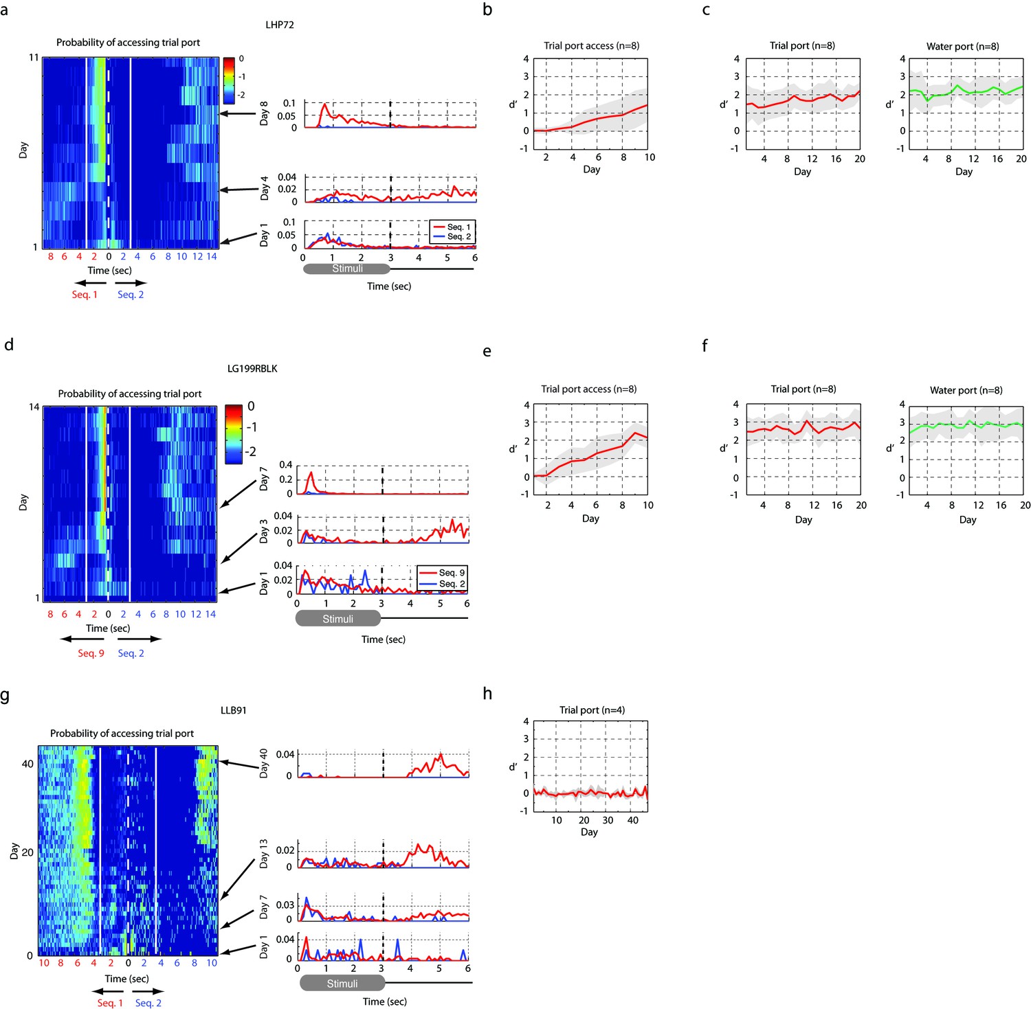
Result of operant training.
(a,b,c) Two-stage training, example of a bird learning sequence 1. (a) The probability distribution of the bird accessing the trial port is shown for the entire training period of the first stage of training (left). The white dotted line represents the start of sequence playback and the white solid line shows the termination time of the stimulus. Any asymmetry between the dotted and solid lines indicates learning (asymmetry implies different behaviors for rewarded and non-rewarded sequences). This bird started to interrupt non-rewarding trials around day 5. Individual rows (specific days in panel (a)) are plotted to the right to illustrate detail. (b) Learning curve for the first stage. Mean d-prime (± s.d.) after ten days of training is shown (n = 8 birds). (c) Learning curve after the passive reward is switched off (the second stage of training). This transition resulted in a minimal change in behavior. (d,e,f) Example of two-stage training for another bird learning a distinct sequence (sequence 9). (d) The probability of accessing the trial port during the first stage of training (left) and three sample days (right). (e) Learning curve at the first stage (n = 8 birds). (f) Learning curve at the second stage (n = 8 birds). (g,h) Example of two-stage training for a sequence whose intervals were slowed by a factor of two. (g) Probability distribution of accessing the trial port during the first stage of training. This bird usually reinitiated trials immediately after the presentation of the click sequence or after drinking water for rewarded trials (note the increased probability of accessing trial port around 10 s). The absence of asymmetry between the dotted and solid lines indicates an absence of learning. (h) Learning curve during the first stage of training. No birds (n = 4 birds in two-stage training) learned to discriminate the slowed click sequences over the course of 40 days of training.
Figure 7
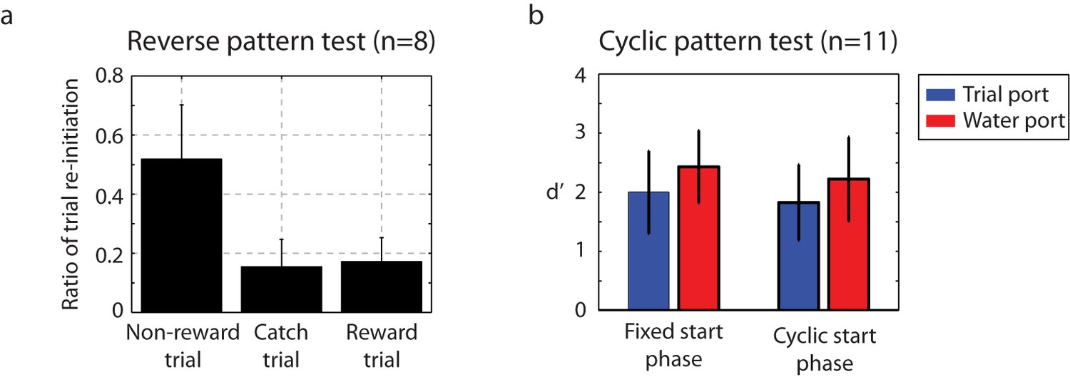
Catch-trial analysis.
(a) During catch-trial analysis, for 10% of non-rewarding trials, we presented reverse patterns to eight birds. The birds did not show any recognition of the reverse pattern (catch trials). Only the familiar non-rewarded sequence led to the adaptive behavior of resetting playback. Mean ± s.d. of trial interruption ratio is shown. (b) In this cyclic permutation catch-trial analysis, playback of the click sequence started at a random interval in the repeating sequence on each trial (a phase shift in the stimulus order); all birds (n = 11) maintained performance. This indicates that discriminations were based on patterns of click intervals regardless of the absolute time of any specific click relative to trial onset.
Figure 8
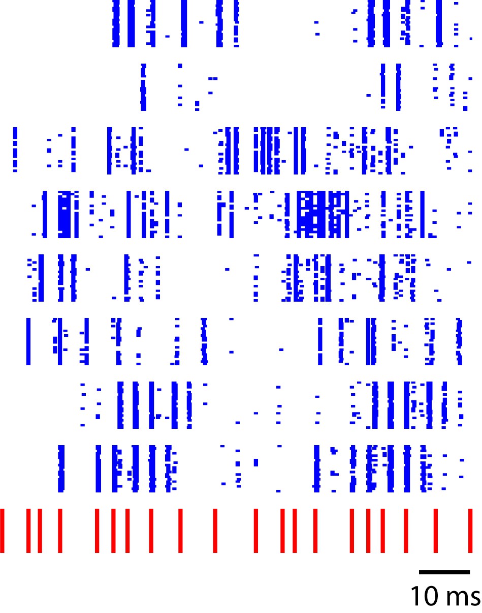
Sequence-selective responses in a critically tuned linear dynamical system.
Each blue row represents simulated neural responses in a simple linear model. The input stimulus (red) has a temporal pattern similar to the click sequences used in this study. This toy model illustrates a temporal to spatial transformation arising from simple linear dynamics in a recurrent system.
Additional files
-
Supplementary file 1
Click-sequence audio files.
We provide audio files of all the click sequences used in this study in .wav format. The last number of the file name corresponds to the index of click sequence. For example, Clk_Sequence_1.wav contains audio data for sequence 1.
- https://doi.org/10.7554/eLife.18205.024
Download links
A two-part list of links to download the article, or parts of the article, in various formats.
Downloads (link to download the article as PDF)
Open citations (links to open the citations from this article in various online reference manager services)
Cite this article (links to download the citations from this article in formats compatible with various reference manager tools)
Transformation of temporal sequences in the zebra finch auditory system
eLife 5:e18205.
https://doi.org/10.7554/eLife.18205


