
The Tutte polynomial is a graph polynomial that encodes a variety of
combinatorial and algebraic information about the graph. It was first
studied by William Tutte[2,3] in 1954 and known as the
dichromatic polynomial since it is a generalization of the chromatic
polynomials introduced by Birkoff[4] and Whitney[5]. The Tutte polynomial is a well-known tool
for examining the characteristics and properties of graphs [6]. The university of the Tutte
polynomial is derived from the recipe theorem (see [7, 8]). The crucial
universal property of this graph polynomial is that practically every
multiplicative graph invariant with a deletion/contraction reduction
must be an evaluation of it[9]. These deletion/contraction operations are
natural reductions for many network models arising from a variety of
problems at the computer science, engineering, statistics, optimization,
and physics.
The Tutte polynomial \(T(G;x,y)\) of a
graph \(G=(V,E)\) is a polynomial in
two variables \(x\) and \(y\). Numerous of graph polynomials are
specially obtained from the Tutte polynomial. For example, the chromatic
polynomial \(P(G;x)\) of \(G\) is a one-variable graph invariant
counts the number of distinct ways to colour \(G\) with \(x\) colours. The Tutte polynomial includes
the chromatic polynomial as a specialization[10, 11, 12]: \[P(G;x) = (-1)^{\left\vert V\right\vert – k(G)}
x^{k(G)} T(G;1-x,0),\] where \(k(G)\) is the number of the connected
components of \(G\).
Also, the flow polynomial \(F(G; y)\)
that counts the number of flows in \(G\) can be derived from the Tutte
polynomial as follows[2]: \[F(G; y) =
(-1)^{\left\vert E\right\vert – \left\vert V\right\vert +k(G)} T(G;0,1-
y)\] Furthermore, the reliability polynomial \(R(G;y)\) of \(G\) is a graph polynomial that measures the
probability that no connected component of \(G\) is disconnected when an edge of \(G\) with fixed probability \(0\leq y \leq 1\), is independently deleted.
The reliability polynomial is also a special polynomial due to the Tutte
polynomial [13]: \[R(G;y) = y^{\left\vert V\right\vert -1}
(1-y)^{\left\vert E\right\vert – \left\vert V\right\vert +1}
T(G;1,\frac{1}{1-y})\] The Tutte polynomials can be defined for
graphs, matrices, and matroids. We concern with finding the Tutte
polynomial for a class of self-similar network. Focusing on self-similar
networks arises from being able to represent some real networks.
Networks with self-similarity property have been studied in various
fields, such as mathematics, computer science, physics, chemistry, and
biology (see[14,15,16,17,18]). There are diverse
and different examples of this networks such as Von Koch graphs,
Sierpinski gasket graphs, and tower of Hanoi graphs (see [19, 20]). Therefore,
calculating the Tutte polynomial for this kind of networks is of a great
interest for many researchers ([24,25,26]).
The Tutte polynomial has evaluations that count a large number of the
graph invariants. The number of acyclic orientation of a graph is a
vital quantity that has many applications in different areas such as
network optimization, social sciences and other fields. For example, the
number of acyclic orientations of a scheduling network equals to the
number of feedback arc set and the number of acyclic orientations of a
social network measures its degree of hierarchy. Also, the number of
acyclic orientations of a network measures its planarity. The number of
acyclic orientations of a graph can be evaluated from the Tutte
polynomial.
Another significant graph invariant is the number of spanning trees that
is related to its structural and dynamical properties. The number of
spanning trees of a self-similar network provides us with information
about the effectiveness of the underlying network. It is well-known that
the number of spanning trees of a graph equals to the determinant of any
cofactor of the Laplacian matrix of the graph. For a graph with a huge
number of nodes, finding analytically the number of spanning trees
becomes harder and harsher. We overcome this difficulty by the aid of
the Tutte polynomial which can enumerate it. Hence, evaluating the
number of spanning trees of a network is considered as a crucial and
fundamental application of the Tutte polynomials.
This paper is organized as follows. In Section 2, we introduce
some definitions and results from graph theory that would be used
throughout the paper and investigate a class of self-similar network
model \(M(t)\). In Section 3, we study
the Tutte polynomial \(T(M(t);x,y)\).
Though determining the Tutte polynomial of a graph is generally an
NP-hard problem, we shall find a recursive formula for the Tutte
polynomial of a network model \(M(t)\)
based on the subgraph decomposition method [21,27,28]. Section 4 is devoted to the
applications of \(T(M(t);x,y)\). We
find the exact formula of the number of acyclic orientations and
spanning trees of network model \(M(t)\). We also discuss the spanning tree
entropy or the asymptotic complexity of \(M(t)\). In section 4, we examine the
self-similar network \(N(t)\) presented
in [1] as another application
of the underlying model \(M(t)\). We
deduce the Tutte polynomial of \(N(t)\)
by applying some results published in[29]. The number of spanning trees of \(N(t)\) is explicitly derived and coincided
with the results obtained by using Matlab code which enhances the
validity of them. Finally, Section 5 gives a brief
summary.
This section briefly presents some necessary definitions that will be used in our calculations. Let \(G=(V(G), E(G))\) be a graph with node set \(V (G)\) and edge set \(E(G)\). The order and size of \(G\) are \(\left\vert V(G)\right\vert\) and \(\left\vert E(G)\right\vert\), respectively. A subgraph \(A=(V(A), E(A))\) of \(G\) is called a spanning subgraph of \(G\) if \(A\) is obtained by edge deletion only, that is, \(V(A) = V(G)\) and \(E(A) \subseteq E(G)\).
The Tutte polynomial is a well-studied invariant of graphs. (For more details, see[11,23]). There are some different but still equivalent definitions of tutte polynomial[8]. Here we introduce the common subgraph extension definition. Let \(A\) be a spanning subgraph of \(G\), then the Tutte polynomial \(T(G;x,y)\) of \(G\) is defined by
\[\label{Tutte} T(G;x,y) = \sum\limits_{A \subseteq G} (x-1)^{k(A)-k(G)}(y-1)^{\left\vert E(A)\right\vert – \left\vert V(A)\right\vert +k(A)},\tag{1}\] where the summation runs over all possible spanning subgraphs \(A\) of \(G\) and \(k(A)\) is the number of connected components of \(A\). From \ref{Tutte}), we notice that theTutte polynomial of \(G\) is a two-variable polynomial in \(x\) and \(y\). It is remarkable that calculating the Tutte polynomial \(T(G;x,y)\) of \(G\) at particular points gives us distinctive combinatorial invariants of \(G\) such that
\(T(G;1,1)=\tau(G)\) is the number of the spanning trees of \(G\).
\(T(G;2,1)=F(G)\) is the number of the spanning forest of \(G\).
\(T(G;1,2)=S(G)\) is the number of the spanning connected subgraphs of \(G\).
\(T(G;2,2) = 2^{\left\vert E(G) \right\vert}\).
\(T(G;2,0)=a(G)\) is the number of acyclic orientations of \(G\).
\(T(G;0,2)=ta(G)\) is the number of totally acyclic orientations of \(G\).
The network model \(M(t)\) can be constructed by an iterative method based on a merging process. The merging process could happen in the following manner.
At any time step \(t\), \(M(t)\) has two special nodes \(a_{t}\) and \(b_{t}\) which are the nodes of the highest degree and an edge \(e_{t}\) connecting them.
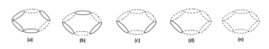
\(M(t+1)\) is obtained by merging 6 copies of \(M(t)\) by joining their special nodes. Merging \(a_{t}\) and \(a_{t}\) gives a new special node \(a_{t+1}\) of \(M(t+1)\) and merging \(b_{t}\) and \(b_{t}\) gives a new special node \(b_{t+1}\) of \(M(t+1)\). The two special nodes \(a_{t+1}\) and \(b_{t+1}\) of \(M(t+1)\) would be linked by a new edge \(e_{t+1}\). The construction process of \(M(t+1)\) is illustrated in Figure 1.
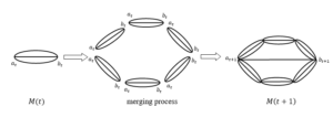
For \(t=0\), let \(M(0)\) be a path with length one whose two endpoints are the special nodes \(a_{0}\) and \(b_{0}\). For \(t\geq 0\), \(M(t+1)\) can be obtained from \(M(t)\) by the construction process presented above, see Figure 2.
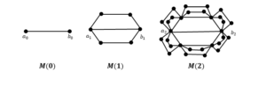
After \(t\) time steps, the order and size of \(M(t)\) are, respectively, \begin{align} \left\vert V(M(t)) \right\vert = \frac{4}{5} 6^{t} +\frac{6}{5} \tag{2} \\ \left\vert E(M(t)) \right\vert = \frac{1}{5} (6^{t+1}-1)\tag{3} \end{align} The solution of average degree of model \(M(t)\) is \[<k(M(t))>~ = \frac{2\left\vert E(M(t))\right\vert}{\left\vert V(M(t))\right\vert}=\frac{\frac{2}{5} (6^{t+1}-1)}{\frac{4}{5} 6^{t} +\frac{6}{5}} \approx 3.\tag{4}\]
The Tutte polynomial of the network model \(M(t)\) is given by \[\label{poly}
T(M(t);x,y) = \sum\limits_{A\subseteq M(t)} (x-1)^{k(A)-1}
(y-1)^{\left\vert E(A)\right\vert-\left\vert
V(A)\right\vert+k(A)}\tag{5}\] Let us categorize the spanning subgraphs
\(A\) of \(M(t)\) into two kinds. The first kind \(\mathcal{M}(1,t)\) is the spanning
subgraphs of \(M(t)\), where the two
special nodes \(a_{t}\) and \(b_{t}\) belong to the same connected
component. The second kind \(\mathcal{M}(2,t)\) is the spanning
subgraphs of \(M(t)\), where the two
special nodes \(a_{t}\) and \(b_{t}\) belong to two different connected
components.
Hence, equation (\ref{poly}) can be rewritten as \[T(M(t);x,y) =T_{1,t}(x,y) +T_{2,t}(x,y),\tag{6}\]
where
\begin{align}
T_{1,t}(x,y) = \sum\limits_{A\subseteq \mathcal{M}(1,t)} (x-1)^{k(A)-1}
(y-1)^{\left\vert E(A)\right\vert-\left\vert V(A)\right\vert+k(A)} \tag{7} \\
T_{2,t}(x,y) = \sum\limits_{A\subseteq \mathcal{M}(2,t)} (x-1)^{k(A)-1}
(y-1)^{\left\vert E(A)\right\vert-\left\vert V(A)\right\vert+k(A)}\tag{8}
\end{align}
To get a recursive formula for \(T(M(t);x,y)\), we will exploit the special
structure of \(M(t+1)\). It is known
that \[T(M(t+1);x,y) = \sum\limits_{A
\subseteq M(t+1)} (x-1)^{k(A)-1} (y-1)^{\left\vert
E(A)\right\vert-\left\vert V(A)\right\vert+k(A)}\tag{9}\] Figure 1
shows that \(M(t+1)\) is created from
six copies of \(M(t)\) by merging some
special nodes and adding an additional edge \(e_{t+1}\). Let the six copies of \(M(t)\) be denoted by \(M_{i}(t), i=1,…,6\). Consequently, let
\(A_{i}\) be a subgraph of \(M_{i}(t), i=1,…,6\), respectively. Define
\(\mathcal{E}\) to be \[\mathcal{E} = \left\{
\begin{array}{c}
\{ e_{t+1} \}\\
\phi
\end{array}
\right.\tag{10}\] As a result, any spanning
subgraph \(A\) of \(M(t+1)\) can be identified by the spanning
subgraphs \(A_{i}\) of the six copies
\(M_{i}(t), i=1,…,6\) with \(\mathcal{E}\). Thus, it is convenient to
express the Tutte polynomial of \(M(t+1)\) as \[T(M(t+1);x,y) = \sum\limits_{A =\left(
\bigcup\limits_{i=1}^{6}A_{i} \right)\cup \mathcal{E}} (x-1)^{k(A)-1}
(y-1)^{\left\vert E(A)\right\vert-\left\vert
V(A)\right\vert+k(A)}\tag{11}\]
Now, we are ready to state the following theorem.
Theorem 1. Tutte polynomial of the model network \(M(t+1)\) is \[\label{main} T(M(t+1);x,y) = T_{1,t+1}(x,y) + (x-1) P_{2,t+1}(x,y),\tag{12}\] where \begin{align} T_{1,t+1}(x,y) = y (y-1)T_{1,t}^{6}(x,y) + 6 y T^{5}_{1,t}(x,y)P_{2,t}(x,y) + (6xy-6y+9)T^{4}_{1,t}(x,y)P_{2,t}^{2}(x,y) \\ + (2x^{2}y-4xy+18x+2y-18)T^{3}_{1,t}(x,y)P_{2,t}^{3}(x,y) + 15(x-1)^{2}T_{1,t}^{2}(x,y)P_{2,t}^{4}(x,y) \\ +6(x-1)^{3}T_{1,t}(x,y) P_{2,t}^{5}(x,y) + (x-1)^{4}P_{2,t}^{6}(x,y) ,\label{Tutte11}\tag{13} \end{align} \begin{align} P_{2,t+1}(x,y) = \frac{T_{2,t+1}(x,y)}{x-1} = 9T_{1,t}^{4}(x,y)P_{2,t}^{2}(x,y) + 18(x-1)T_{1,t}^{3}(x,y)P_{2,t}^{3}(x,y) \\ +15(x-1)^{2}T_{1,t}^{2}(x,y)P_{2,t}^{4}(x,y)+6(x-1)^{3}T_{1,t}(x,y)P_{2,t}^{5}(x,y)+(x-1)^{4}P_{2,t}^{6}(x,y),\label{Tutte2}\tag{14} \end{align} with initial conditions \(T_{1,0}(x,y)=1\) and \(P_{2,0}(x,y)=1\).
Proof. The initial conditions are obvious since \(M(0)\) is a path of length one. To prove relations (\ref{main}), (\ref{Tutte11}), and (\ref{Tutte2}), we need to investigate all possible spanning subgraphs \(A\) of \(M(t+1)\) and analyze their corresponding contributions to \(T(M(t+1);x,y)\).
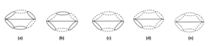
Let’s start with spanning subgraphs where the special nodes \(a_{t+1}\) and \(b_{t+1}\) belong to the same component. There are 13 distinguish configurations of spanning subgraphs \(A\) satisfying this property. Figures 3, 4 and 5 show the possible configurations associated with their contributions. We find that \[\begin{gathered} T_{1,t+1}(x,y) = y(y-1)T_{1,t}^{6} + \frac{6y}{x-1}T_{1,t}^{5}T_{2,t} + \frac{6xy+9}{(x-1)^{2}}T_{1,t}^{4}T_{2,t}^{2} \\ + \frac{2xy+16}{(x-1)^{2}}T_{1,t}^{3}T_{2,t}^{3} + \frac{15}{(x-1)^{2}}T_{1,t}^{2}T_{2,t}^{4} + \frac{6}{(x-1)^{2}}T_{1,t}T_{2,t}^{5} + \frac{1}{(x-1)^{2}}T^{6}_{2,t} ~~~~~~ \end{gathered}\]
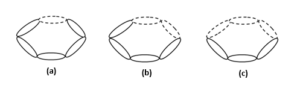
Let’s discuss the spanning subgraphs where the special nodes \(a_{t+1}\) and \(b_{t+1}\) belong to two different components. There are 5 different configurations of spanning trees \(A\) with the above mentioned property. Figure 6 depicts this case. We also get \[\begin{gathered} T_{2,t+1}(x,y) = \frac{9}{x-1}T_{1,t}^{4}T_{2,t}^{2} + \frac{18}{x-1}T_{1,t}^{3}T_{2,t}^{3} + \frac{15}{x-1}T_{1,t}^{2}T_{2,t}^{4} + \frac{6}{x-1}T_{1,t}T_{2,t}^{5} + \frac{1}{x-1}T_{2,t}^{6}. \end{gathered}\]

It is clear that \(x-1\) divides \(T_{2,t}(x,y),~ t \geq 0\). Thus, we put \(T_{2,t}(x,y) = (x-1)P_{2,t}(x,y)\) and the proof is completed.
Many graph invarients can be simply obtained from the Tutte polynomial of the graph. In what comes, we shall exploit some evaluations of the Tutte polynomial of the proposed model.
The number of acyclic orientations \(a(G)\) of a graph \(G\) is a crucial quantity in graph theory with related applications in various areas such as social sciences, optimization, computer science and other fields[22]. Stanley[30] studied the relation between \(a(G)\) and the chromatic polynomial \(P(G;x)\). It is also known that \(a(G)\) can be calculated by the aid of the Tutte polynomial since \(a(G)=T(G;2,0)\). Therefore we shall apply this result to our model \(M(t)\) to get an explicit formula for \(a(M(t))\).
Theorem 2. The number of acyclic orientations of \(M(t)\) is given by \[a(M(t)) = 2\times 49^{\frac{1}{5}(6^{t}-1)}.\tag{15}\]
Proof. Since \[T(G;2,0) = a(G).\] Thus, we put \(x=2, y=0\) in (\ref{main}) \[a(M(t+1)) = T(M(t+1);2,0) = T_{1,t+1}(2,0)+P_{2,t+1}(2,0)\] From (\ref{Tutte11}) and (\ref{Tutte2}), we find that \[T_{1,t+1}(2,0) = P_{2,t+1}(2,0),\] and \[\label{acyclic} T_{1,t+1}(2,0) = 49 T_{1,t}^{6}(2,0),\tag{16}\] with initial condition \(T_{1,0}(2,0)=1\). Solving [acyclic], we get \[T_{1,t}(2,0)=49^{\frac{1}{5}(6^{t}-1)}.\] This completes the required result.
We shall evaluate an explicit formula for the number of spanning trees of network model \(M(t)\) as an application of the Tutte polynomial of \(M(t)\).
Theorem 3. The number of spanning trees of \(M(t)\) is given by \[\tau(M(t)) = 3\lambda_{t}^{4} (3+2\lambda_{t}) \prod\limits_{k=0}^{t-2} (9\lambda_{t-k-1}^{4})^{6^{k+1}},\tag{17}\] where \(\lambda_{t} = 3(1-(\frac{2}{3})^t)\).
Proof. It is a renowned result that \[T(G;1,1) = \tau(G).\] Thus, we put \(x=y=1\) in (\ref{main}) \[\tau(M(t+1)) = T(M(t+1);1,1) =
T_{1,t+1}(1,1)\] From (\ref{Tutte11}) and
(\ref{Tutte2}), we have system of difference
equations in the form
\begin{eqnarray}
\tau(M(t+1)) &=& 6\tau^{5}(M(t))P_{2,t}(1,1) + 9 \tau^{4}(M(t))P_{2,t}^{2}(1,1) \tag{18}\label{no1} \\
P_{2,t+1}(1,1) &=& 9\tau^{4}(M(t))P_{2,t}^{2}(1,1), \tag{19} \label{no2}
\end{eqnarray}
with initial conditions \(\tau(M(0)) = P_{2,0}(1,1) = 1\).
Using (\ref{no1}) and (\ref{no2}), we can deduce
that \[\begin{aligned}
\frac{\tau(M(t))}{P_{2,t}(1,1)} &=& 1 + \frac{2}{3}
\frac{\tau(M(t-1))}{P_{2,t-1}(1,1)}
=
3\left(1-\left(\frac{2}{3}\right)^{t+1}\right)
\end{aligned}\] We can say that \[\tau(M(t)) = \lambda_{t+1} P_{2,t}(1,1),\]
where \(\lambda_{t} =
3\left(1-\left(\frac{2}{3}\right)^{t}\right)\). Now, we
substitute in (\ref{no2}) \[\begin{aligned}
P_{2,t}(1,1) &=& 9\lambda_{t}^{4}P_{2,t-1}^{6}(1,1)
= 9\lambda_{t}^{4} \left( 9 \lambda_{t-1}^{4}
P_{2,t-2}^{6}(1,1) \right)^{6}
= \left( 9\lambda_{t}^{4} \right) \left(
9\lambda_{t-1}^{4} \right)^6 … \left( 9
\lambda^{4}_{t-k+1} \right)^{6^{k-1}} P_{2,t-k}^{6^k}(1,1) \\
&=& \prod\limits_{k=0}^{t-1} \left(
9\lambda_{t-k}^{4} \right)^{6^k}
\end{aligned}\] Back to (\ref{no2}), we find that \[\begin{aligned}
\tau(M(t)) &=& 9\lambda_{t}^{4} P_{2,t-1}^{6}(1,1) + 6
\lambda_{t}^{5} P_{2,t-1}^{6}(1,1)
= 3\lambda_{t}^{4}(3+2\lambda_{t}) P_{2,t-1}^{6}
= 3\lambda_{t}^{4}(3+2\lambda_{t})
\prod\limits_{k=0}^{t-2} \left( 9\lambda_{t-k-1}^{4} \right)^{6^{k+1}}.
\end{aligned}\]
The entropy of spanning trees or asymptotic complexity of any graph network is a graph invarient which measures the robustness of the graph. We can say that the higher the entropy of spanning trees, the higher the robustness of the graph.
Theorem 4. The spanning trees entropy of model \(M(t)\) is given by \[\rho(M(t)) = \lim\limits_{\left\vert V(M(t)) \right\vert\rightarrow \infty} \frac{\ln \tau(M(t))}{\left\vert V(M(t)) \right\vert} \approx 0.64\tag{20}\]
Proof. We have \[\begin{aligned} \rho(M(t)) &=& \lim\limits_{\left\vert V(M(t)) \right\vert\rightarrow \infty} \frac{\ln \tau(M(t))}{\left\vert V(M(t)) \right\vert} = \lim\limits_{t \rightarrow \infty} \frac{\ln \left(3\lambda_{t}^{4}(3+2\lambda_{t}) \prod\limits_{k=0}^{t-2} \left( 9\lambda_{t-k-1}^{4} \right)^{6^{k+1}} \right)}{\frac{4}{5}6^t +\frac{6}{5}} \\ &\approx& \lim\limits_{t \rightarrow \infty} \frac{6^{t-3}\ln 9\lambda_{3}^{4} + 6^{t-2} \ln 9\lambda_{2}^{4} + 6^{t-1} \ln 9\lambda_{1}^{4}}{\frac{4}{5}6^t } \approx 0.64. \end{aligned}\]
The network model \(N(t)\) has been presented in [1] and it can be obtained from the network model \(M(t)\) by replacing each edge in \(M(t)\) by a path of length 2 as shown in Figure 7.
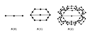
As presented, the network model \(N(t)\), studied in[1], is obtained from the network model \(M(t)\) by replacing each edge in \(M(t)\) by a path of length two. We can also
deduce the Tutte polynomial of \(N(t)\)
by the aid of the Tutte polynomial of \(M(t)\) based on the results published in
[29].
We shall rely on the work achieved by Y. Liao et al. [29] to compute the Tutte
polynomial of model \(N(t)\).
Theorem 5. The Tutte polynomial of the network model \(N(t)\) is given by \[T(N(t);x,y) = (1+x)^{\frac{2}{5}\left(6^{t}-1\right)} T\left(M(t);x^{2},\frac{y+x}{1+x}\right).\tag{21}\]
As a result, we will evaluate the number of spanning trees of \(N(t)\) and compare it with the main result presented by Ma et al. [1]. In [1], a formula for calculating the number of spanning trees was presented in Theorem 6 which isn’t redress. In the following, we display the correct formula for calculating the number of spanning trees in Theorem 1. A total verification with more points of interest than the one displayed in[1] is given.
Theorem 6. The number of spanning trees of the network model \(N(t)\) is given by \[\tau(N(t)) = 2^{\frac{2}{5}\left(6^{t}-1\right)} \tau(M(t)).\tag{22}\]
Note that this result is inconsistent with the previous work [1]. We will verify the accuracy of our result by using Matlab package (R2019a). The numerical examples were run on a computer with an Intel(R) processor running at 2.50 GHz using 8.00 GB of RAM, running Windows.
| \(t\) | \(\tau(N(t))\) (our results) | \(\tau(N(t))\) (results in[1]) | \(\tau(N(t))\) (Matlab results) |
|---|---|---|---|
| 0 | 1 | 1 | 1 |
| 1 | 60 | 60 | 60 |
| 2 | \(1.2765\times 10^{12}\) | \(1.3201\times 10^{11}\) | \(1.2765\times 10^{12}\) |
| 3 | \(8.4134\times 10^{73}\) | \(6.7730\times 10^{66}\) | \(8.4134\times 10^{73}\) |
Table 1 shows the number of spanning trees of \(N(t)\) for the first forth values of \(t\). Initially, at \(t=0,1\), our results, the results from [1], and numerical results from Matlab code are identical. Whereas at \(t=2,3\), our results are the same as the results obtained from Matlab code, and differ with the results proposed in [1].
Self-similar networks are hugely investigated in many fields of studies. Numerous of the characteristics and properties of self-similar networks can be recognized from the Tutte polynomial. The Tutte polynomial of graphs is a considerable graph invariant that includes other graph invariants as a specialization. We find that the Tutte polynomial of two self-similar networks, namely \(M(t)\) and \(N(t)\). In particular, the exact formulae of the number of the spanning trees of both of them are deduced. Furthermore, we find that our formula of the number of spanning trees of \(N(t)\) is more correct than the formula presented by Ma et al.[1].
Data availability: Not applicable.
Conflicts of interests: The authors declare that they have no conflicting of interests.
Author’s contributions: AWA suggested the considered problem. FE analyzed the problem and was a major contributer in writing the manuscript. All authors read and approved the final manuscript.
Funding: Not applicable.
The authors declare no conflict of interests.