
Enhancing Green Supply Chain Efficiency Through Linear Diophantine Fuzzy Soft-Max Aggregation Operators
Abstract:
Improving the effectiveness of green supply chains is a critical step towards minimizing waste, optimizing resource use, and reducing the environmental impact of business operations. Sustainable practices should be implemented throughout the entire supply chain, from product design and procurement to production and transportation, in order to achieve these goals. By doing so, businesses can not only improve their environmental performance but also reduce costs, increase customer satisfaction, and gain a competitive advantage in the market. However, due to the existence of competing characteristics, imprecise information, and a lack of knowledge, selecting the appropriate green provider is a complex and unpredictable decision-making issue. The primary objective of a linear-diophantine fuzzy (LiDF) framework is to assist decision makers in selecting the optimal course of action. This paper introduces several novel aggregation operators (AOs), namely the linear Diophantine fuzzy soft-max average (LiDFSMA) and the linear Diophantine fuzzy soft-max geometric (LiDFSMG) operators. The proposed method is then demonstrated through a simple example of a green supplier optimization technique containing linear Diophantine fuzzy content, showing the utility and applicability of the approach. Overall, the proposed LiDF framework and AOs can aid decision makers in selecting the most suitable green provider, thereby enhancing the efficiency of green supply chains.
1. Introduction
In every aspect of life, including academic, personal, and professional spheres, the ability to make decisions is essential. The process of selecting the optimal course of action from a number of alternatives based on a predetermined set of criteria is known as decision-making. Effective decision-making can have a significant impact on an individual’s success in achieving their goals, as well as on the performance and profitability of an organization. It involves analyzing and evaluating information, considering alternatives, and making rational decisions based on available evidence. Developing strong decision-making skills is essential for success in both personal and professional lives.
In ecological supply chain management, decision-making is crucial for achieving objectives. Decision-making involves identifying objectives, evaluating available alternatives, and selecting the best course of action. In green supply chains, decision-makers must consider environmental concerns, such as reducing pollution and emissions, using renewable energy, and minimizing environmental impact. Decision-makers in green supply chains face the challenge of balancing environmental and economic considerations. In some cases, environmentally responsible alternatives may be more expensive than conventional ones. For example, renewable energy may be more expensive than conventional energy sources in the short term. The costs must be weighed against the benefits of environmental sustainability to determine the best course of action.
Accurate and timely information is crucial for effective decision-making in ecological supply chains. This information may come from various sources, including suppliers, consumers, and internal data systems. Data analytics can help decision-makers analyze this data and identify patterns and trends that can inform their decisions. For example, data analytics can be used to determine the most environmentally responsible suppliers, reducing the environmental impact of procurement. Collaboration is another essential element of effective decision-making in green supply chains. To achieve shared goals, collaboration requires supply chain stakeholders to exchange information and resources. Collaboration can assist organizations in identifying areas where they can reduce waste and increase productivity by cooperating. For example, suppliers and manufacturers can collaborate to reduce packaging waste and optimize transportation routes, respectively.
The problem of imprecise and misleading data has been a recurrent issue in numerous disciplines, including business, management, social, medical, technological, emotional, and machine learning. Data aggregation is essential for decision-making; however, the uncertainty of data makes data aggregation problematic. Multi-criteria decision-making (MCDM) is a cognitive activity tool frequently used to choose among a finite number of alternatives based on the preference information provided by decision-makers (DMs). Due to the complexity of human reasoning abilities, MCDM tends to be erroneous and ambiguous, making it difficult for DMs to provide accurate evaluations during the review process. Therefore, it is imperative to resolve this problem and deal with unpredictability.
Zadeh was a pioneer of fuzzy set (FS) theory as an alternative to crisp numbers or linguistic numbers [1]. Atanassov introduced the novel idea of intuitionistic fuzzy sets (IFS) [2], [3], while Yager extended it to Pythagorean fuzzy sets (PFS) [4], [5], [6]. Yager also introduced the concept of q-ROFS, which is a further generalization of IFS and PFS [7]. However, the limitation of q-ROFS is that the total of the membership degree (MD) power and the non-membership degree (NMD) power of q may be less than or identical to one.
Numerous decision-making approaches for various extensions of fuzzy sets have been proposed by Alcantud and Garcia [8], Xu [9] and Xu and Yager [10], Wang and Liu [11], Zhang et al. [12], Zhao et al. [13] and Garg [14]. Mahmood et al. [15] proposed a spherical fuzzy decision-making approach with a diagnosis application. Feng et al. [16], Peng and Yang [17], Zhang and Xu [18], and Riaz et al. [19], [20], [21], [22] proposed various decision-making techniques. Simic et al. [23], [24] conducted extensive work in this area.
Riaz and Hashmi [19] introduced the concept of LiDFS as a generalized approach of IFS, PFS, and q-ROFS. LiDFS is a new technique for analyzing uncertain decision-making, computational maximizing efficiency, and realworld situations using reference parameters. Work related to LiDFS is presented in [20], [21], [22]. Riaz et al. [25], [26], [27], [28], [29], [30], [31] introduced the concept of bipolar picture fuzzy. Simic et al. [23] introduced the normalized weighted geometric Dombi Bonferoni mean operator with interval grey numbers, while Pamucar and Jankovic Riaz et al. [24] established the hybrid interval rough weighted power-Heronian operator for MCDM.
Decision-makers often struggle with evaluating diverse alternatives due to the restrictions on the sum of membership and non-membership degrees of IFSs, PFSs, and q-ROFS. To overcome this limitation, the LiDFS theory has been suggested, which allows decision-makers to select grades freely ranging from 0 to 1 due to the presence of reference parameters. However, there is currently no tool available to deal with a linear prioritized relationship among the criterion in LiDF data. To address this gap in research, several types of soft-max AOs have been proposed to aggregate LiDF data. These AOs can significantly enhance the efficiency of green supply chains by facilitating decision-making processes and providing accurate evaluations.
The remaining sections of this paper are organized as follows. Section 2 covers fundamental LiDFS concepts. Section 3 develops various LiDF soft-max AOs. The fourth and fifth sections present an MCDM framework for the suggested AOs, along with a numerical example. Finally, this section summarizes the main findings of the research paper.
2. Preliminaries
In this part, we will go over some of the more important fundamental aspects of LiDFS.
Definition 2.1. [19] A LiDFS $\Re$ in $\beth$ is defined as
$\Re=\big\{\big(\triangledown,\langle \mathfrak{Y}_{\Re}(\triangledown),\mathfrak{X}_{\Re}(\triangledown)\rangle,\langle \mathfrak{D}_{\Re}(\triangledown),\mathfrak{Z}_{\Re}(\triangledown)\rangle\big):\triangledown\in \beth\big\},$
where, $\mathfrak{Y}_{\Re}(\triangledown),\mathfrak{X}_{\Re}(\triangledown),\mathfrak{D}_{\Re}(\triangledown),\mathfrak{Z}_{\Re}(\triangledown)\in[0,1]$ are the MD, the NMD and the corresponding "reference parameters (RPs)", respectively. Moreover,
$0\leq\mathfrak{D}_{\Re}(\triangledown)+\mathfrak{Z}_{\Re}(\triangledown)\leq1,$
and
$0\leq\mathfrak{D}_{\Re}(\triangledown)\mathfrak{Y}_{\Re}(\triangledown)+\mathfrak{Z}_{\Re}(\triangledown)\mathfrak{X}_{\Re}(\triangledown)\leq1$
for all $\triangledown\in\beth$. The LiDFS
${\Re_\beth}=\{(\triangledown,\langle1,0\rangle,\langle1,0\rangle):\triangledown\in\beth\}$
is known the absolute LiDFS in $\beth$. The LiDFS
${\Re_\phi}=\{(\triangledown,\langle0,1\rangle,\langle0,1\rangle):\triangledown\in\beth\}$
is known the null LiDFS in $\beth$. The RPs may be utilised to characterise or categorise particular structures. By altering the physical significance of the reference parameters, it is possible to categorise various systems.
Definition 2.2. [19] A "linear Diophantine fuzzy number" (LiDFN) is a tuple ${\hbar^{\gamma}}=(\langle\mathfrak{Y}_{{\hbar^{\gamma}}},\mathfrak{X}_{{\hbar^{\gamma}}}\rangle,\langle\mathfrak{D}_{{\hbar^{\gamma}}},\mathfrak{Z}_{{\hbar^{\gamma}}}\rangle)$ satisfying the following conditions:
(1) $0 \leq \mathfrak{Y}_{\hbar^\gamma}, \mathfrak{X}_{\hbar^\gamma}, \mathfrak{D}_{\hbar^\gamma}, \mathfrak{Z}_{\hbar^\gamma} \leq 1$;
(2) $0 \leq \mathfrak{D}_{\hbar^\gamma}+\mathfrak{Z}_{\hbar^\gamma} \leq 1$;
(3) $0 \leq \mathfrak{D}_{\hbar^\gamma} \mathfrak{Y}_{\hbar^\gamma}+\mathfrak{Z}_{\hbar^\gamma} \mathfrak{X}_{\hbar^\gamma} \leq 1$.
Definition 2.3. [19] Let ${\hbar^{\gamma}}=(\langle \mathfrak{Y}_{{\hbar^{\gamma}}}, \mathfrak{X}_{{\hbar^{\gamma}}}\rangle,\langle\mathfrak{D}_{{\hbar^{\gamma}}},\mathfrak{Z}_{{\hbar^{\gamma}}}\rangle)$ be a LiDFN, then score function $\maltese({\hbar^{\gamma}})$ can be define by the mapping $\maltese({\hbar^{\gamma}}):LiDFN(\beth)\rightarrow[-1,1]$ and given by
$\maltese({\hbar^{\gamma}})=\frac{1}{2}[(\mathfrak{Y}_{{\hbar^{\gamma}}}-\mathfrak{X}_{{\hbar^{\gamma}}})+(\mathfrak{D}_{{\hbar^{\gamma}}}-\mathfrak{Z}_{{\hbar^{\gamma}}})]$
where $LiDFN(\beth)$ is an assemblage of LiDFNs on $\beth$.
Definition 2.4. [19] Let ${\hbar^{\gamma}}=(\langle \mathfrak{Y}_{{\hbar^{\gamma}}}, \mathfrak{X}_{{\hbar^{\gamma}}} \rangle,\langle\mathfrak{D}_{{\hbar^{\gamma}}},\mathfrak{Z}_{{\hbar^{\gamma}}}\rangle)$ be a LiDFN, then accuracy function can be defined by the mapping $\psi:LiDFN(\beth)\rightarrow[0,1]$ and given as
$\psi({\hbar^{\gamma}})=\frac{1}{2}\Big[\Big(\frac{\mathfrak{Y}_{{\hbar^{\gamma}}}+\mathfrak{X}_{{\hbar^{\gamma}}}}{2}\Big)+(\mathfrak{D}_{{\hbar^{\gamma}}}+\mathfrak{Z}_{{\hbar^{\gamma}}})\Big]$
Definition 2.5. [19] Let ${\hbar^{\gamma}}_1$ and ${\hbar^{\gamma}}_2$ be two LiDFNs then by using the score function and accuracy function, we have:
(i): If $\maltese({\hbar^{\gamma}}_1)<\maltese({\hbar^{\gamma}}_2)$ then $ {\hbar^{\gamma}}_1 < {\hbar^{\gamma}}_2$,
(ii): If $\maltese({\hbar^{\gamma}}_2)<\maltese({\hbar^{\gamma}}_1)$ then $ {\hbar^{\gamma}}_2 < {\hbar^{\gamma}}_1$,
(iii): If $\maltese({\hbar^{\gamma}}_2) = \maltese({\hbar^{\gamma}}_1)$ then,
(a): If $\psi({\hbar^{\gamma}}_1)<\psi({\hbar^{\gamma}}_2)$ then $ {\hbar^{\gamma}}_1 < {\hbar^{\gamma}}_2$,
(b): If $\psi({\hbar^{\gamma}}_2)<\psi({\hbar^{\gamma}}_1)$ then $ {\hbar^{\gamma}}_2 < {\hbar^{\gamma}}_1$,
(c): If $\psi({\hbar^{\gamma}}_1) = \psi({\hbar^{\gamma}}_2)$ then ${\hbar^{\gamma}}_1 = {\hbar^{\gamma}}_2$.
Definition 2.6. [19] Let ${\hbar^{\gamma}}=(\langle \mathfrak{Y}_{{\hbar^{\gamma}}}, \mathfrak{X}_{{\hbar^{\gamma}}}\rangle,\langle\mathfrak{D}_{{\hbar^{\gamma}}},\mathfrak{Z}_{{\hbar^{\gamma}}}\rangle)$ be a LiDFN, another definition of score function is defined as expectation score function (ESF) on $LiDFN(\beth)$ having range $\mathfrak{H}:LiDFN(\beth)\rightarrow[0,1]$ and define as
$\mathfrak{H}({\hbar^{\gamma}})=\frac{1}{2}\Big[\frac{(\mathfrak{Y}_{{\hbar^{\gamma}}}-\mathfrak{X}_{{\hbar^{\gamma}}}+1)}{2}+\frac{(\mathfrak{D}_{{\hbar^{\gamma}}}-\mathfrak{Z}_{{\hbar^{\gamma}}}+1)}{2}\Big]$
Definition 2.7. [19] Let ${\hbar^{\gamma}}_{i}=(\langle\mathfrak{Y}_{i},\mathfrak{X}_{i}\rangle,\langle\mathfrak{D}_{i},\mathfrak{Z}_{i}\rangle)$ be two LiDFNs with $i=1,2$. Then
$\bullet$ ${\hbar^{\gamma}}_{1}\subseteq {\hbar^{\gamma}}_{2} \Leftrightarrow \mathfrak{Y}_{1}\leq\mathfrak{Y}_{2},\mathfrak{X}_{2}\leq\mathfrak{X}_{1}, \mathfrak{D}_{1}\leq \mathfrak{D}_{2}, \mathfrak{Z}_{2}\leq \mathfrak{Z}_{1}$;
$\bullet$ ${\hbar^{\gamma}}_{1}={\hbar^{\gamma}}_{2} \Leftrightarrow \mathfrak{Y}_{1}=\mathfrak{Y}_{2},\mathfrak{X}_{1}=\mathfrak{X}_{2},\mathfrak{D}_{1}=\mathfrak{D}_{2}, \mathfrak{Z}_{1}=\mathfrak{Z}_{2}$;
$\bullet$ ${\hbar^{\gamma}}_{1}\oplus{\hbar^{\gamma}}_{2}=\left(\langle\mathfrak{Y}_{1}+\mathfrak{Y}_{2}-\mathfrak{Y}_{1}\mathfrak{Y}_{2},\mathfrak{X}_{1}\mathfrak{X}_{2}\rangle,\langle\mathfrak{D}_{1}+\mathfrak{D}_{2}-\mathfrak{D}_{1}\mathfrak{D}_{2},\mathfrak{Z}_{1}\mathfrak{Z}_{2}\rangle\right)$;
$\bullet$ ${\hbar^{\gamma}}_{1}\otimes{\hbar^{\gamma}}_{2}=\left(\langle\mathfrak{Y}_{1}\mathfrak{Y}_{2},\mathfrak{X}_{1}+\mathfrak{X}_{2}-\mathfrak{X}_{1}\mathfrak{X}_{2}\rangle,\langle\mathfrak{D}_{1}\mathfrak{D}_{2},\mathfrak{Z}_{1}+\mathfrak{Z}_{2}-\mathfrak{Z}_{1}\mathfrak{Z}_{2}\rangle\right)$.
$\bullet$ ${\hbar^{\gamma}}^c_{1}=(\langle\mathfrak{X}_{1},\mathfrak{Y}_{1}\rangle,\langle\mathfrak{Z}_{1},\mathfrak{D}_{1}\rangle)$;
$\bullet$ $\mathfrak{X}{\hbar^{\gamma}}_{1}=\left(\langle1-(1-\mathfrak{Y}_{1})^\mathfrak{X},\mathfrak{X}_{1}^{\mathfrak{X}}\rangle,\langle1-(1-\mathfrak{D}_{1})^\mathfrak{X},\mathfrak{Z}_{1}^{\mathfrak{X}}\rangle\right)$;
$\bullet$ ${\hbar^{\gamma}}_{1}^{\mathfrak{X}}=\left(\langle\mathfrak{Y}_{1}^\mathfrak{X},1-(1-\mathfrak{X}_{1})^{\mathfrak{X}}\rangle,\langle\mathfrak{D}_{1}^\mathfrak{X},1-(1-\mathfrak{Z}_{1})^{\mathfrak{X}}\rangle\right)$.
In the discipline of mathematics, the soft-max function is a kind of generalization that is derived from the logistic function. It has been gradually used in a wide variety of areas of study, including, for example, computer vision and strategic planning. The following is a representation of the soft-max function in its mathematical equation:
$\phi_k\left(j, \vartheta_1, \vartheta_2, \ldots, \vartheta_n\right)=\phi_k^j=\frac{\exp \left(\vartheta_j / k\right)}{\sum_{j=1}^n \exp \left(\vartheta_j / k\right)}, k>0$
For the LiDFNs ${\hbar^{\gamma}}_j(j=1,2,3, \ldots, n), S_j$ is the score value of LiDFN ${\hbar^{\gamma}}_j$. Every $\vartheta_j$ is formulated by given the equation.
$\vartheta_j= \begin{cases}\prod_{i=1}^{j-1} S_i, \mathrm{j}=2,3, \ldots, n \\ 1 & \mathrm{j}=1\end{cases}$
where, $k$ is the modulation parameter.
3. LDF Soft-Max AOs
This section introduces the concepts of LiDFSMA operator and LiDFSMG operator.
Definition 3.1. Assume that $ {\hbar^{\gamma}}_{\gimel} = ( \langle \mathfrak{Y}_{\gimel}, \mathfrak{X}_{\gimel}\rangle,\langle\mathfrak{D}_{\gimel},\mathfrak{Z}_{\gimel} \rangle )$ is the assemblage of LiDFNs, and $ \text{LiDFSMA}: £^n \rightarrow £ $, be a n dimension mapping. if
then the mapping LiDFSMA is called LiDFSMA operator, where $ {\aleph^{\hbar}}_{\gimel}= \overline{\prod}_{k=1}^{j-1} \mathfrak{H}({\hbar^{\gamma}}_k) $ $(j=2 \ldots, n )$, ${\aleph^{\hbar}}_1 = 1$ and $\mathfrak{H}({\hbar^{\gamma}}_k)$ is the expectation score function of $k^{th}$ LiDFN. We could also think about LiDFSMA operators using the following theory, which is based on the operational law of LiDFN.
Theorem 3.2. Assume that $\hbar^{\gamma}_{\beth}=\left(\left\langle\mathfrak{Y}_{\beth}, \mathfrak{X}_{\beth}\right\rangle,\left\langle\mathfrak{D}_{\beth}, \mathfrak{Z}_{\jmath}\right\rangle\right)$ is the assemblage of LiDFNs, we can find LiDFSMA by
Proof. Definition 3.1 and Theorem 3.2 are easily preceded by the first statement. This is shown in the following aspects.
$\text{LiDFSMA}({\hbar^{\gamma}}_{1} , {\hbar^{\gamma}}_{2},\ldots {\hbar^{\gamma}}_{n} ) = \Bigg( \frac{ \displaystyle \exp [ {\aleph^{\hbar}}_1/ ~\eth ]}{ \displaystyle \sum_{\gimel=1}^{n} \exp [{\aleph^{\hbar}}_{\gimel} / ~\eth ] } {\hbar^{\gamma}}_{1} \oplus \frac{ \displaystyle \exp [ {\aleph^{\hbar}}_2/ ~\eth ]}{ \displaystyle \sum_{\gimel=1}^{n} \exp [{\aleph^{\hbar}}_{\gimel} / ~\eth ] } {\hbar^{\gamma}}_{2} \oplus \ldots, \frac{ \exp [ {\aleph^{\hbar}}_n/ ~\eth ]}{ \displaystyle \sum_{\gimel=1}^{n} \exp [{\aleph^{\hbar}}_{\gimel} / ~\eth ] } {\hbar^{\gamma}}_{n} \Bigg)$
$= \Bigg( \Bigg \langle 1- \prod_{\gimel=1}^n(1-\mathfrak{Y}_{\gimel})^{\frac{ \displaystyle \exp [ {\aleph^{\hbar}}_{\gimel}/ ~\eth ]}{ \displaystyle \sum_{\gimel=1}^{n} \exp [{\aleph^{\hbar}}_{\gimel} / ~\eth ] }}, \prod_{\gimel=1}^n \mathfrak{X}_{\gimel}^{\frac{ \displaystyle \exp [ {\aleph^{\hbar}}_{\gimel}/ ~\eth ]}{ \displaystyle \sum_{\gimel=1}^{n} \exp [{\aleph^{\hbar}}_{\gimel} / ~\eth ] }} \Bigg \rangle,$
$\Bigg \langle \prod_{\gimel=1}^n(1-\mathfrak{D}_{\gimel})^{\frac{ \displaystyle \exp [ {\aleph^{\hbar}}_{\gimel}/ ~\eth ]}{ \displaystyle \sum_{\gimel=1}^{n} \exp [{\aleph^{\hbar}}_{\gimel} / ~\eth ] }}, \qquad \prod_{\gimel=1}^n \mathfrak{Z}_{\gimel}^{\frac{ \displaystyle \exp [ {\aleph^{\hbar}}_{\gimel}/ ~\eth ]}{ \displaystyle \sum_{\gimel=1}^{n} \exp [{\aleph^{\hbar}}_{\gimel} / ~\eth ] }} \Bigg \rangle \Bigg)$
We used mathematical induction to prove this theorem.
For n=2
$\frac{ \displaystyle \exp [ {\aleph^{\hbar}}_1/ ~\eth ]}{ \displaystyle \sum_{\gimel=1}^{n} \exp [{\aleph^{\hbar}}_{\gimel} / ~\eth ] } {\hbar^{\gamma}}_{1} = \Bigg( \Bigg \langle 1- (1-\mathfrak{Y}_1)^{\frac{ \displaystyle \exp [ {\aleph^{\hbar}}_1/ ~\eth ]}{ \displaystyle \sum_{\gimel=1}^{n} \exp [{\aleph^{\hbar}}_{\gimel} / ~\eth ] }}, \mathfrak{X}_1^{\frac{ \displaystyle \exp [ {\aleph^{\hbar}}_1/ ~\eth ]}{ \displaystyle \sum_{\gimel=1}^{n} \exp [{\aleph^{\hbar}}_{\gimel} / ~\eth ] }} \Bigg \rangle,$
$\Bigg \langle 1- (1-\mathfrak{D}_1)^{\frac{ \displaystyle \exp [ {\aleph^{\hbar}}_1/ ~\eth ]}{ \displaystyle \sum_{\gimel=1}^{n} \exp [{\aleph^{\hbar}}_{\gimel} / ~\eth ] }}, \mathfrak{Z}_1^{\frac{ \displaystyle \exp [ {\aleph^{\hbar}}_1/ ~\eth ]}{ \displaystyle \sum_{\gimel=1}^{n} \exp [{\aleph^{\hbar}}_{\gimel} / ~\eth ] }} \Bigg \rangle \Bigg)$
$\frac{ \displaystyle \exp [ {\aleph^{\hbar}}_2/ ~\eth ]}{ \displaystyle \sum_{\gimel=1}^{n} \exp [{\aleph^{\hbar}}_{\gimel} / ~\eth ] } \\ {\hbar^{\gamma}}_{2} = \Bigg( \Bigg \langle 1- (1-\mathfrak{Y}_2)^{\frac{ \displaystyle \exp [ {\aleph^{\hbar}}_1/ ~\eth ]}{ \displaystyle \sum_{\gimel=1}^{n} \exp [{\aleph^{\hbar}}_{\gimel} / ~\eth ] }}, \mathfrak{X}_2^{\frac{ \displaystyle \exp [ {\aleph^{\hbar}}_1/ ~\eth ]}{ \displaystyle \sum_{\gimel=1}^{n} \exp [{\aleph^{\hbar}}_{\gimel} / ~\eth ] }} \Bigg \rangle,$
$\Bigg \langle 1- (1-\mathfrak{D}_2)^{\frac{ \displaystyle \exp [ {\aleph^{\hbar}}_1/ ~\eth ]}{ \displaystyle \sum_{\gimel=1}^{n} \exp [{\aleph^{\hbar}}_{\gimel} / ~\eth ] }}, \mathfrak{Z}_2^{\frac{ \displaystyle \exp [ {\aleph^{\hbar}}_1/ ~\eth ]}{ \displaystyle \sum_{\gimel=1}^{n} \exp [{\aleph^{\hbar}}_{\gimel} / ~\eth ] }} \Bigg \rangle \Bigg)$
Then
$ \frac{ \displaystyle \exp [ {\aleph^{\hbar}}_1/ ~\eth ]}{ \displaystyle \sum_{\gimel=1}^{n} \exp [{\aleph^{\hbar}}_{\gimel} / ~\eth ] } {\hbar^{\gamma}}_{1} \oplus \frac{ \displaystyle \exp [ {\aleph^{\hbar}}_2/ ~\eth ]}{ \displaystyle \sum_{\gimel=1}^{n} \exp [{\aleph^{\hbar}}_{\gimel} / ~\eth ] } {\hbar^{\gamma}}_{2} $
$= \Bigg( \Bigg \langle 1- (1-\mathfrak{Y}_1)^{\frac{ \displaystyle \exp [ {\aleph^{\hbar}}_1/ ~\eth ]}{ \displaystyle \sum_{\gimel=1}^{n} \exp [{\aleph^{\hbar}}_{\gimel} / ~\eth ] }}, \mathfrak{X}_1^{\frac{ \displaystyle \exp [ {\aleph^{\hbar}}_1/ ~\eth ]}{ \displaystyle \sum_{\gimel=1}^{n} \exp [{\aleph^{\hbar}}_{\gimel} / ~\eth ] }} \Bigg \rangle,$
$\Bigg \langle 1- (1-\mathfrak{D}_1)^{\frac{ \displaystyle \exp [ {\aleph^{\hbar}}_1/ ~\eth ]}{ \displaystyle \sum_{\gimel=1}^{n} \exp [{\aleph^{\hbar}}_{\gimel} / ~\eth ] }}, \mathfrak{Z}_1^{\frac{ \displaystyle \exp [ {\aleph^{\hbar}}_1/ ~\eth ]}{ \displaystyle \sum_{\gimel=1}^{n} \exp [{\aleph^{\hbar}}_{\gimel} / ~\eth ] }} \Bigg \rangle \Bigg) \oplus$
$\Bigg( \Bigg \langle 1- (1-\mathfrak{Y}_2)^{\frac{ \displaystyle \exp [ {\aleph^{\hbar}}_1/ ~\eth ]}{ \displaystyle \sum_{\gimel=1}^{n} \exp [{\aleph^{\hbar}}_{\gimel} / ~\eth ] }}, \mathfrak{X}_2^{\frac{ \displaystyle \exp [ {\aleph^{\hbar}}_1/ ~\eth ]}{ \displaystyle \sum_{\gimel=1}^{n} \exp [{\aleph^{\hbar}}_{\gimel} / ~\eth ] }} \Bigg \rangle,$
$\Bigg \langle 1- (1-\mathfrak{D}_2)^{\frac{ \displaystyle \exp [ {\aleph^{\hbar}}_1/ ~\eth ]}{ \displaystyle \sum_{\gimel=1}^{n} \exp [{\aleph^{\hbar}}_{\gimel} / ~\eth ] }}, \mathfrak{Z}_2^{\frac{ \displaystyle \exp [ {\aleph^{\hbar}}_1/ ~\eth ]}{ \displaystyle \sum_{\gimel=1}^{n} \exp [{\aleph^{\hbar}}_{\gimel} / ~\eth ] }} \Bigg \rangle \Bigg)$
$= \Bigg( \Bigg \langle 1- (1-\mathfrak{Y}_1)^{\frac{ \displaystyle \exp [ {\aleph^{\hbar}}_1/ ~\eth ]}{ \displaystyle \sum_{\gimel=1}^{n} \exp [{\aleph^{\hbar}}_{\gimel} / ~\eth ] }} + 1- (1-\mathfrak{Y}_2)^{\frac{ \displaystyle \exp [ {\aleph^{\hbar}}_1/ ~\eth ]}{ \displaystyle \sum_{\gimel=1}^{n} \exp [{\aleph^{\hbar}}_{\gimel} / ~\eth ] }}$
$- \Bigg((1- (1-\mathfrak{Y}_1)^{\frac{ \displaystyle \exp [ {\aleph^{\hbar}}_1/ ~\eth ]}{ \displaystyle \sum_{\gimel=1}^{n} \exp [{\aleph^{\hbar}}_{\gimel} / ~\eth ] }} \Bigg) \Bigg( (1- (1-\mathfrak{Y}_2)^{\frac{ \displaystyle \exp [ {\aleph^{\hbar}}_1/ ~\eth ]}{ \displaystyle \sum_{\gimel=1}^{n} \exp [{\aleph^{\hbar}}_{\gimel} / ~\eth ] }} \Bigg),$
$\mathfrak{X}_1^{\frac{ \displaystyle \exp [ {\aleph^{\hbar}}_1/ ~\eth ]}{ \displaystyle \sum_{\gimel=1}^{n} \exp [{\aleph^{\hbar}}_{\gimel} / ~\eth ] }} . \mathfrak{X}_2^{\frac{ \displaystyle \exp [ {\aleph^{\hbar}}_1/ ~\eth ]}{ \displaystyle \sum_{\gimel=1}^{n} \exp [{\aleph^{\hbar}}_{\gimel} / ~\eth ] }} \Bigg \rangle, \Bigg \langle 1- (1-\mathfrak{D}_1)^{\frac{ \displaystyle \exp [ {\aleph^{\hbar}}_1/ ~\eth ]}{ \displaystyle \sum_{\gimel=1}^{n} \exp [{\aleph^{\hbar}}_{\gimel} / ~\eth ] }} + 1- (1-\mathfrak{D}_2)^{\frac{ \displaystyle \exp [ {\aleph^{\hbar}}_1/ ~\eth ]}{ \displaystyle \sum_{\gimel=1}^{n} \exp [{\aleph^{\hbar}}_{\gimel} / ~\eth ] }} -$
$\Bigg( (1- (1-\mathfrak{D}_1)^{\frac{ \displaystyle \exp [ {\aleph^{\hbar}}_1/ ~\eth ]}{ \displaystyle \sum_{\gimel=1}^{n} \exp [{\aleph^{\hbar}}_{\gimel} / ~\eth ] }} \Bigg) \Bigg(1- (1-\mathfrak{D}_2)^{\frac{ \displaystyle \exp [ {\aleph^{\hbar}}_1/ ~\eth ]}{ \displaystyle \sum_{\gimel=1}^{n} \exp [{\aleph^{\hbar}}_{\gimel} / ~\eth ] }} \Bigg),$
$\mathfrak{Z}_1^{\frac{ \displaystyle \exp [ {\aleph^{\hbar}}_1/ ~\eth ]}{ \displaystyle \sum_{\gimel=1}^{n} \exp [{\aleph^{\hbar}}_{\gimel} / ~\eth ] }} . \mathfrak{Z}_2^{\frac{ \displaystyle \exp [ {\aleph^{\hbar}}_1/ ~\eth ]}{ \displaystyle \sum_{\gimel=1}^{n} \exp [{\aleph^{\hbar}}_{\gimel} / ~\eth ] }} \Bigg \rangle \Bigg)$
$= \Bigg( \Bigg \langle 1 - (1-\mathfrak{Y}_1)^{\frac{ \displaystyle \exp [ {\aleph^{\hbar}}_1/ ~\eth ]}{ \displaystyle \sum_{\gimel=1}^{n} \exp [{\aleph^{\hbar}}_{\gimel} / ~\eth ] }} (1-\mathfrak{Y}_2)^{\frac{ \displaystyle \exp [ {\aleph^{\hbar}}_1/ ~\eth ]}{ \displaystyle \sum_{\gimel=1}^{n} \exp [{\aleph^{\hbar}}_{\gimel} / ~\eth ] }} , \mathfrak{X}_1^{\frac{ \displaystyle \exp [ {\aleph^{\hbar}}_1/ ~\eth ]}{ \displaystyle \sum_{\gimel=1}^{n} \exp [{\aleph^{\hbar}}_{\gimel} / ~\eth ] }} . \mathfrak{X}_2^{\frac{ \displaystyle \exp [ {\aleph^{\hbar}}_1/ ~\eth ]}{ \displaystyle \sum_{\gimel=1}^{n} \exp [{\aleph^{\hbar}}_{\gimel} / ~\eth ] }} \Bigg \rangle,$
$\langle 1 - (1-\mathfrak{D}_1)^{\frac{ \displaystyle \exp [ {\aleph^{\hbar}}_1/ ~\eth ]}{ \displaystyle \sum_{\gimel=1}^{n} \exp [{\aleph^{\hbar}}_{\gimel} / ~\eth ] }} (1-\mathfrak{D}_2)^{\frac{ \displaystyle \exp [ {\aleph^{\hbar}}_1/ ~\eth ]}{ \displaystyle \sum_{\gimel=1}^{n} \exp [{\aleph^{\hbar}}_{\gimel} / ~\eth ] }} , \mathfrak{Z}_1^{\frac{ \displaystyle \exp [ {\aleph^{\hbar}}_1/ ~\eth ]}{ \displaystyle \sum_{\gimel=1}^{n} \exp [{\aleph^{\hbar}}_{\gimel} / ~\eth ] }} . \mathfrak{Z}_2^{\frac{ \displaystyle \exp [ {\aleph^{\hbar}}_1/ ~\eth ]}{ \displaystyle \sum_{\gimel=1}^{n} \exp [{\aleph^{\hbar}}_{\gimel} / ~\eth ] }} \Bigg \rangle \Bigg)$
$= \Bigg( \Bigg \langle 1 - \prod_{\gimel=1}^2 (1-\mathfrak{Y}_{\gimel})^{\frac{ \displaystyle \exp [ {\aleph^{\hbar}}_{\gimel}/ ~\eth ]}{ \displaystyle \sum_{\gimel=1}^{n} \exp [{\aleph^{\hbar}}_{\gimel} / ~\eth ] }} , \prod_{\gimel=1}^2 \mathfrak{X}_{\gimel}^{\frac{ \displaystyle \exp [ {\aleph^{\hbar}}_{\gimel}/ ~\eth ]}{ \displaystyle \sum_{\gimel=1}^{n} \exp [{\aleph^{\hbar}}_{\gimel} / ~\eth ] }} \Bigg \rangle,$
$\Bigg \langle 1 - \prod_{\gimel=1}^2 (1-\mathfrak{D}_{\gimel})^{\frac{ \displaystyle \exp [ {\aleph^{\hbar}}_{\gimel}/ ~\eth ]}{ \displaystyle \sum_{\gimel=1}^{n} \exp [{\aleph^{\hbar}}_{\gimel} / ~\eth ] }} , \prod_{\gimel=1}^2 \mathfrak{Z}_{\gimel}^{\frac{ \displaystyle \exp [ {\aleph^{\hbar}}_{\gimel}/ ~\eth ]}{ \displaystyle \sum_{\gimel=1}^{n} \exp [{\aleph^{\hbar}}_{\gimel} / ~\eth ] }} \Bigg \rangle \Bigg)$
This reveals that Eq. 2 is valid for n=2; now suppose that Eq. 2 is true for n=k, i.e.,
$\text{LiDFSMA}({\hbar^{\gamma}}_{1} , {\hbar^{\gamma}}_{2},\ldots {\hbar^{\gamma}}_{k} )= \Bigg( \Bigg \langle 1- \prod_{\gimel=1}^k(1-\mathfrak{Y}_{\gimel})^{\frac{ \displaystyle \exp [ {\aleph^{\hbar}}_{\gimel}/ ~\eth ]}{ \displaystyle \sum_{\gimel=1}^{n} \exp [{\aleph^{\hbar}}_{\gimel} / ~\eth ] }}, \prod_{\gimel=1}^k \mathfrak{X}_{\gimel}^{\frac{ \displaystyle \exp [ {\aleph^{\hbar}}_{\gimel}/ ~\eth ]}{ \displaystyle \sum_{\gimel=1}^{n} \exp [{\aleph^{\hbar}}_{\gimel} / ~\eth ] }} \Bigg \rangle,$
$\Bigg \langle 1- \prod_{\gimel=1}^k(1-\mathfrak{D}_{\gimel})^{\frac{ \displaystyle \exp [ {\aleph^{\hbar}}_{\gimel}/ ~\eth ]}{ \displaystyle \sum_{\gimel=1}^{n} \exp [{\aleph^{\hbar}}_{\gimel} / ~\eth ] }}, \prod_{\gimel=1}^k \mathfrak{Z}_{\gimel}^{\frac{ \displaystyle \exp [ {\aleph^{\hbar}}_{\gimel}/ ~\eth ]}{ \displaystyle \sum_{\gimel=1}^{n} \exp [{\aleph^{\hbar}}_{\gimel} / ~\eth ] }} \Bigg \rangle \Bigg)$
Now n=k+1, by operational laws of LiDFNs we have,
$\text{LiDFSMA}({\hbar^{\gamma}}_{1} , {\hbar^{\gamma}}_{2},\ldots {\hbar^{\gamma}}_{k+1} )= \text{LiDFSMA}({\hbar^{\gamma}}_{1} , {\hbar^{\gamma}}_{2},\ldots {\hbar^{\gamma}}_{k} ) \oplus \frac{ \displaystyle \exp [ {\aleph^{\hbar}}_{\gimel}/ ~\eth ]}{ \displaystyle \sum_{\gimel=1}^{n} \exp [{\aleph^{\hbar}}_{\gimel} / ~\eth ] } {\hbar^{\gamma}}_{k+1}$
$=\Bigg( \Bigg \langle 1- \prod_{\gimel=1}^k(1-\mathfrak{Y}_{\gimel})^{\frac{ \displaystyle \exp [ {\aleph^{\hbar}}_{\gimel}/ ~\eth ]}{ \displaystyle \sum_{\gimel=1}^{n} \exp [{\aleph^{\hbar}}_{\gimel} / ~\eth ] }}, \prod_{\gimel=1}^k \mathfrak{X}_{\gimel}^{\frac{ \displaystyle \exp [ {\aleph^{\hbar}}_{\gimel}/ ~\eth ]}{ \displaystyle \sum_{\gimel=1}^{n} \exp [{\aleph^{\hbar}}_{\gimel} / ~\eth ] }} \Bigg \rangle,$
$\Bigg \langle 1- \prod_{\gimel=1}^k(1-\mathfrak{D}_{\gimel})^{\frac{ \displaystyle \exp [ {\aleph^{\hbar}}_{\gimel}/ ~\eth ]}{ \displaystyle \sum_{\gimel=1}^{n} \exp [{\aleph^{\hbar}}_{\gimel} / ~\eth ] }}, \prod_{\gimel=1}^k \mathfrak{Z}_{\gimel}^{\frac{ \displaystyle \exp [ {\aleph^{\hbar}}_{\gimel}/ ~\eth ]}{ \displaystyle \sum_{\gimel=1}^{n} \exp [{\aleph^{\hbar}}_{\gimel} / ~\eth ] }} \Bigg \rangle \Bigg) \oplus$
$\Bigg( \Bigg \langle 1- (1-\mathfrak{Y}_{k+1})^{\frac{ \displaystyle \exp [ {\aleph^{\hbar}}_{k+1}/ ~\eth ]}{ \displaystyle \sum_{\gimel=1}^{n} \exp [{\aleph^{\hbar}}_{\gimel} / ~\eth ] }}, \mathfrak{X}_{k+1}^{\frac{ \displaystyle \exp [ {\aleph^{\hbar}}_{k+1}/ ~\eth ]}{ \displaystyle \sum_{\gimel=1}^{n} \exp [{\aleph^{\hbar}}_{\gimel} / ~\eth ] }} \Bigg \rangle,$
$\Bigg \langle 1- (1-\mathfrak{D}_{k+1})^{\frac{ \displaystyle \exp [ {\aleph^{\hbar}}_{k+1}/ ~\eth ]}{ \displaystyle \sum_{\gimel=1}^{n} \exp [{\aleph^{\hbar}}_{\gimel} / ~\eth ] }}, \mathfrak{Z}_{k+1}^{\frac{ \displaystyle \exp [ {\aleph^{\hbar}}_{k+1}/ ~\eth ]}{ \displaystyle \sum_{\gimel=1}^{n} \exp [{\aleph^{\hbar}}_{\gimel} / ~\eth ] }} \Bigg \rangle \Bigg)$
$=\Bigg( \Bigg \langle 1- \prod_{\gimel=1}^k (1-\mathfrak{Y}_k)^{\frac{ \displaystyle \exp [ {\aleph^{\hbar}}_{\gimel}/ ~\eth ]}{ \displaystyle \sum_{\gimel=1}^{n} \exp [{\aleph^{\hbar}}_{\gimel} / ~\eth ] }} + 1- (1-\mathfrak{Y}_{k+1})^{\frac{ \displaystyle \exp [ {\aleph^{\hbar}}_{k+1}/ ~\eth ]}{ \displaystyle \sum_{\gimel=1}^{n} \exp [{\aleph^{\hbar}}_{\gimel} / ~\eth ] }}$
$- \Bigg( 1- \prod_{\gimel=1}^k (1-\mathfrak{Y}_k)^{\frac{ \displaystyle \exp [ {\aleph^{\hbar}}_{\gimel}/ ~\eth ]}{ \displaystyle \sum_{\gimel=1}^{n} \exp[{\aleph^{\hbar}}_{\gimel} / ~\eth ] }} \Bigg)\Bigg( 1- (1-\mathfrak{Y}_{k+1})^{\frac{ \displaystyle \exp [ {\aleph^{\hbar}}_{k+1}/ ~\eth ]}{ \displaystyle \sum_{\gimel=1}^{n} \exp [{\aleph^{\hbar}}_{\gimel} / ~\eth ] }} \Bigg),$
$\prod_{\gimel=1}^k \mathfrak{X}_k^{\frac{ \displaystyle \exp [ {\aleph^{\hbar}}_{\gimel}/ ~\eth ]}{ \displaystyle \sum_{\gimel=1}^{n} \exp [{\aleph^{\hbar}}_{\gimel} / ~\eth ] }} . \mathfrak{X}_{k=1}^{\frac{ \displaystyle \exp [ {\aleph^{\hbar}}_{k+1}/ ~\eth ]}{ \displaystyle \sum_{\gimel=1}^{n} \exp [{\aleph^{\hbar}}_{\gimel} / ~\eth ] }} \Bigg \rangle,$
$\Bigg \langle 1- \prod_{\gimel=1}^k (1-\mathfrak{D}_k)^{\frac{ \displaystyle \exp [ {\aleph^{\hbar}}_{\gimel}/ ~\eth ]}{ \displaystyle \sum_{\gimel=1}^{n} \exp [{\aleph^{\hbar}}_{\gimel} / ~\eth ] }} + 1- (1-\mathfrak{D}_{k+1})^{\frac{ \displaystyle \exp [ {\aleph^{\hbar}}_{k+1}/ ~\eth ]}{ \displaystyle \sum_{\gimel=1}^{n} \exp [{\aleph^{\hbar}}_{\gimel} / ~\eth ] }} -$
$\Bigg( 1- \prod_{\gimel=1}^k (1-\mathfrak{D}_k)^{\frac{ \displaystyle \exp [ {\aleph^{\hbar}}_{\gimel}/ ~\eth ]}{ \displaystyle \sum_{\gimel=1}^{n} \exp [{\aleph^{\hbar}}_{\gimel} / ~\eth ] }} \Bigg) \Bigg( 1- (1-\mathfrak{D}_{k+1})^{\frac{ \displaystyle \exp [ {\aleph^{\hbar}}_{k+1}/ ~\eth ]}{ \displaystyle \sum_{\gimel=1}^{n} \exp [{\aleph^{\hbar}}_{\gimel} / ~\eth ] }} \Bigg) ,$
$\prod_{\gimel=1}^k \mathfrak{Z}_k^{\frac{ \displaystyle \exp [ {\aleph^{\hbar}}_{\gimel}/ ~\eth ]}{ \displaystyle \sum_{\gimel=1}^{n} \exp [{\aleph^{\hbar}}_{\gimel} / ~\eth ] }} . \mathfrak{Z}_{k=1}^{\frac{ \displaystyle \exp [ {\aleph^{\hbar}}_{k+1}/ ~\eth ]}{ \displaystyle \sum_{\gimel=1}^{n} \exp [{\aleph^{\hbar}}_{\gimel} / ~\eth ] }} \Bigg \rangle \Bigg)$
$= \Bigg(\Bigg \langle 1- \prod_{\gimel=1}^k (1-\mathfrak{Y}_k)^{\frac{ \displaystyle \exp [ {\aleph^{\hbar}}_{\gimel}/ ~\eth ]}{ \displaystyle \sum_{\gimel=1}^{n} \exp [{\aleph^{\hbar}}_{\gimel} / ~\eth ] }} (1-\mathfrak{Y}_{k+1})^{\frac{ \displaystyle \exp [ {\aleph^{\hbar}}_{k+1}/ ~\eth ]}{ \displaystyle \sum_{\gimel=1}^{n} \exp [{\aleph^{\hbar}}_{\gimel} / ~\eth ] }},$
$\prod_{\gimel=1}^k \mathfrak{X}_k^{\frac{ \displaystyle \exp [ {\aleph^{\hbar}}_{\gimel}/ ~\eth ]}{ \displaystyle \sum_{\gimel=1}^{n} \exp [{\aleph^{\hbar}}_{\gimel} / ~\eth ] }} . \mathfrak{X}_{k+1}^{\frac{ \displaystyle \exp [ {\aleph^{\hbar}}_{k+1}/ ~\eth ]}{ \displaystyle \sum_{\gimel=1}^{n} \exp [{\aleph^{\hbar}}_{\gimel} / ~\eth ] }} \Bigg \rangle$
$\Bigg \langle 1- \prod_{\gimel=1}^k (1-\mathfrak{D}_k)^{\frac{ \displaystyle \exp [ {\aleph^{\hbar}}_{\gimel}/ ~\eth ]}{ \displaystyle \sum_{\gimel=1}^{n} \exp [{\aleph^{\hbar}}_{\gimel} / ~\eth ] }} (1-\mathfrak{D}_{k+1})^{\frac{ \displaystyle \exp [ {\aleph^{\hbar}}_{k+1}/ ~\eth ]}{ \displaystyle \sum_{\gimel=1}^{n} \exp [{\aleph^{\hbar}}_{\gimel} / ~\eth ] }},$
$\prod_{\gimel=1}^k \mathfrak{Z}_k^{\frac{ \displaystyle \exp [ {\aleph^{\hbar}}_{\gimel}/ ~\eth ]}{ \displaystyle \sum_{\gimel=1}^{n} \exp [{\aleph^{\hbar}}_{\gimel} / ~\eth ] }} . \mathfrak{Z}_{k+1}^{\frac{ \displaystyle \exp [ {\aleph^{\hbar}}_{k+1}/ ~\eth ]}{ \displaystyle \sum_{\gimel=1}^{n} \exp [{\aleph^{\hbar}}_{\gimel} / ~\eth ] }} \Bigg \rangle \Bigg)$
$=\Bigg( \Bigg \langle 1- \prod_{\gimel=1}^{k+1}(1-\mathfrak{Y}_{\gimel})^{\frac{ \displaystyle \exp [ {\aleph^{\hbar}}_{k+1}/ ~\eth ]}{ \displaystyle \sum_{\gimel=1}^{n} \exp [{\aleph^{\hbar}}_{\gimel} / ~\eth ] }}, \prod_{\gimel=1}^{k+1} \mathfrak{X}_{\gimel}^{\frac{ \displaystyle \exp [ {\aleph^{\hbar}}_{\gimel}/ ~\eth ]}{ \displaystyle \sum_{\gimel=1}^{n} \exp [{\aleph^{\hbar}}_{\gimel} / ~\eth ] }} \Bigg \rangle,$
$\Bigg \langle 1- \prod_{\gimel=1}^{k+1}(1-\mathfrak{D}_{\gimel})^{\frac{ \displaystyle \exp [ {\aleph^{\hbar}}_{k+1}/ ~\eth ]}{ \displaystyle \sum_{\gimel=1}^{n} \exp [{\aleph^{\hbar}}_{\gimel} / ~\eth ] }}, \prod_{\gimel=1}^{k+1} \mathfrak{Z}_{\gimel}^{\frac{ \displaystyle \exp [ {\aleph^{\hbar}}_{\gimel}/ ~\eth ]}{ \displaystyle \sum_{\gimel=1}^{n} \exp [{\aleph^{\hbar}}_{\gimel} / ~\eth ] }} \Bigg \rangle \Bigg)$
This shows that for n = k+1, Eq. 2 holds. Then,
$\text{LiDFSMA}({\hbar^{\gamma}}_{1} , {\hbar^{\gamma}}_{2},\ldots {\hbar^{\gamma}}_{n} )=\Bigg( \Bigg \langle 1- \prod_{\gimel=1}^n(1-\mathfrak{Y}_{\gimel})^{\frac{ \displaystyle \exp [ {\aleph^{\hbar}}_{\gimel}/ ~\eth ]}{ \displaystyle \sum_{\gimel=1}^{n} \exp [{\aleph^{\hbar}}_{\gimel} / ~\eth ] }}, \prod_{\gimel=1}^n \mathfrak{X}_{\gimel}^{\frac{ \displaystyle \exp [ {\aleph^{\hbar}}_{\gimel}/ ~\eth ]}{ \displaystyle \sum_{\gimel=1}^{n} \exp [{\aleph^{\hbar}}_{\gimel} / ~\eth ] }} \Bigg \rangle$
$\Bigg \langle 1- \prod_{\gimel=1}^n(1-\mathfrak{D}_{\gimel})^{\frac{ \displaystyle \exp [ {\aleph^{\hbar}}_{\gimel}/ ~\eth ]}{ \displaystyle \sum_{\gimel=1}^{n} \exp [{\aleph^{\hbar}}_{\gimel} / ~\eth ] }}, \prod_{\gimel=1}^n \mathfrak{Z}_{\gimel}^{\frac{ \displaystyle \exp [ {\aleph^{\hbar}}_{\gimel}/ ~\eth ]}{ \displaystyle \sum_{\gimel=1}^{n} \exp [{\aleph^{\hbar}}_{\gimel} / ~\eth ] }} \Bigg \rangle \Bigg)$
A few of LiDFSMA’s promising properties are described below.
Theorem 3.3. Assume that $ {\hbar^{\gamma}}_{\gimel} = ( \langle \mathfrak{Y}_{\gimel}, \mathfrak{X}_{\gimel} \rangle , \langle \mathfrak{D}_{\gimel}, \mathfrak{Z}_{\gimel} \rangle ) $ is the assemblage of LiDFNs, where ${\aleph^{\hbar}}_{\gimel}= \prod_{k=1}^{j-1} \mathfrak{H}({\hbar^{\gamma}}_k) $ $(j=2 \ldots, n )$, ${\aleph^{\hbar}}_1 = 1$ and $\mathfrak{H}({\hbar^{\gamma}}_k)$ is the expectation score function of $k^{th}$ LiDFN. If all $ {\hbar^{\gamma}}_{\gimel} $ are equal, i.e., $ {\hbar^{\gamma}}_{\gimel}= {\hbar^{\gamma}}$for all j, then
$ \text{LiDFSMA}({\hbar^{\gamma}}_{1} , {\hbar^{\gamma}}_{2},\ldots {\hbar^{\gamma}}_{n} )= {\hbar^{\gamma}} $
Proof. From Definition 3.1, we have
$\text{LiDFSMA}({\hbar^{\gamma}}_{1}, {\hbar^{\gamma}}_{2},\ldots {\hbar^{\gamma}}_{n}) = \frac{ \displaystyle \exp [ {\aleph^{\hbar}}_1/ ~\eth ]}{ \displaystyle \sum_{\gimel=1}^{n} \exp [{\aleph^{\hbar}}_{\gimel} / ~\eth ] } {\hbar^{\gamma}}_{1} \oplus \frac{ \displaystyle \exp [ {\aleph^{\hbar}}_2/ ~\eth ]}{ \displaystyle \sum_{\gimel=1}^{n} \exp [{\aleph^{\hbar}}_{\gimel} / ~\eth ] } {\hbar^{\gamma}}_{2} \oplus \ldots, \oplus \frac{ \exp [ {\aleph^{\hbar}}_n/ ~\eth ]}{ \displaystyle \sum_{\gimel=1}^{n} \exp [{\aleph^{\hbar}}_{\gimel} / ~\eth ] } {\hbar^{\gamma}}_{n}$
$= \frac{ \displaystyle \exp [ {\aleph^{\hbar}}_1/ ~\eth ]}{ \displaystyle \sum_{\gimel=1}^{n} \exp [{\aleph^{\hbar}}_{\gimel} / ~\eth ] } {\hbar^{\gamma}} \oplus \frac{ \displaystyle \exp [ {\aleph^{\hbar}}_2/ ~\eth ]}{ \displaystyle \sum_{\gimel=1}^{n} \exp [{\aleph^{\hbar}}_{\gimel} / ~\eth ] } {\hbar^{\gamma}} \oplus \ldots , \oplus \frac{ \exp [ {\aleph^{\hbar}}_n/ ~\eth ]}{ \displaystyle \sum_{\gimel=1}^{n} \exp [{\aleph^{\hbar}}_{\gimel} / ~\eth ] } {\hbar^{\gamma}}= {\hbar^{\gamma}}$
Corollary 3.4. If ${\hbar^{\gamma}}_{\gimel} = ( \langle \mathfrak{Y}_{\gimel}, \mathfrak{X}_{\gimel} \rangle , \langle \mathfrak{D}_{\gimel}, \mathfrak{Z}_{\gimel} \rangle)$, $j=(1, 2, \ldots n) $ is the assemblage of largest LiDFNs, i.e., $ {\hbar^{\gamma}}_{\gimel}= (1, 0)$ for all j, then
$\text{LiDFSMA}({\hbar^{\gamma}}_{1} , {\hbar^{\gamma}}_{2},\ldots {\hbar^{\gamma}}_{n} )= (\langle1, 0\rangle, \langle 1, 0 \rangle)$
Proof. We can easily obtain Corollary similar to the Theorem 3.3.
Corollary 3.5. (Non-compensatory) If $ {\hbar^{\gamma}}_{1} = ( \langle \mathfrak{Y}_{1}, \mathfrak{X}_{1} \rangle , \langle \mathfrak{D}_{1}, \mathfrak{Z}_{1} \rangle ) $ is the smallest LiDFN, i.e,. $ {\hbar^{\gamma}}_{1}= (\langle0, 1\rangle, \langle 0, 1 \rangle)$, then
$\text{LiDFSMA}({\hbar^{\gamma}}_{1} , {\hbar^{\gamma}}_{2},\ldots {\hbar^{\gamma}}_{n} )= (\langle0, 1\rangle, \langle 0, 1 \rangle)$
Proof. Here, $ {\hbar^{\gamma}}_{1}= (\langle0, 1\rangle, \langle 0, 1 \rangle) $ then by definition of the score function, we have,
$\mathfrak{H}({\hbar^{\gamma}}_{1})=0$
Since,
${\aleph^{\hbar}}_{\gimel}= \prod_{k=1}^{j-1} \mathfrak{H}({\hbar^{\gamma}}_k) \qquad (j=2 \ldots, n ), \quad \text{and} \quad {\aleph^{\hbar}}_1 = 1 $
$\mathfrak{H}({\hbar^{\gamma}}_k)$ is the score of $k^{th}$ LiDFN.
We have,
${\aleph^{\hbar}}_{\gimel}= \prod_{k=1}^{j-1} \mathfrak{H}({\hbar^{\gamma}}_k) = \mathfrak{H}({\hbar^{\gamma}}_1) \times \mathfrak{H}({\hbar^{\gamma}}_2) \times \ldots \times \mathfrak{H}({\hbar^{\gamma}}_{j-1})= 0 \times \mathfrak{H}({\hbar^{\gamma}}_2) \times \ldots \times \mathfrak{H}({\hbar^{\gamma}}_{j-1}) \qquad (j=2 \ldots, n ) $
$ \prod_{k=1}^{j} {\aleph^{\hbar}}_{\gimel}= 1 $
From Definition 3.1, we have
$\text{LiDFSMA}({\hbar^{\gamma}}_{1} , {\hbar^{\gamma}}_{2},\ldots {\hbar^{\gamma}}_{n} ) = \frac{ \displaystyle \exp [ {\aleph^{\hbar}}_1/ ~\eth ]}{ \displaystyle \sum_{\gimel=1}^{n} \exp [{\aleph^{\hbar}}_{\gimel} / ~\eth ] } {\hbar^{\gamma}}_{1} \oplus \frac{ \displaystyle \exp [ {\aleph^{\hbar}}_2/ ~\eth ]}{ \displaystyle \sum_{\gimel=1}^{n} \exp [{\aleph^{\hbar}}_{\gimel} / ~\eth ] } {\hbar^{\gamma}}_{2} \oplus \ldots ,$
$\oplus \frac{ \exp [ {\aleph^{\hbar}}_n/ ~\eth ]}{ \displaystyle \sum_{\gimel=1}^{n} \exp [{\aleph^{\hbar}}_{\gimel} / ~\eth ] } {\hbar^{\gamma}}_{n}= \frac{1}{1} {\hbar^{\gamma}}_{1} \oplus \frac{0}{1} {\hbar^{\gamma}}_{2} \oplus \ldots \frac{0}{1} {\hbar^{\gamma}}_{n}= {\hbar^{\gamma}}_{1} = (0, 1)$
The corollary 3.5 implied that if the higher priority requirements were met by the smallest LiDFN, incentives would not be given to other criteria, even if they were met.
Corollary 3.6. (Monotonicity) Assume that $ {\hbar^{\gamma}}_{\gimel} = ( \langle \mathfrak{Y}_{\gimel}, \mathfrak{X}_{\gimel} \rangle , \langle \mathfrak{D}_{\gimel}, \mathfrak{Z}_{\gimel} \rangle ) $ and $ {\hbar^{\gamma}}^*_{\gimel} = (\langle \mathfrak{Y}^*_{\gimel}, \mathfrak{X}^*_{\gimel} \rangle, \langle \mathfrak{D}^*_{\gimel}, \mathfrak{Z}^*_{\gimel} \rangle )$ are the assemblages of LiDFNs, where ${\aleph^{\hbar}}_{\gimel}= \prod_{k=1}^{j-1} \mathfrak{H}({\hbar^{\gamma}}_k) $, ${\aleph^{\hbar}}^*_{\gimel}= \prod_{k=1}^{j-1} \mathfrak{H}({\hbar^{\gamma}}^*_k) $ $(j=2 \ldots, n )$, ${\aleph^{\hbar}}_1 = 1$, ${\aleph^{\hbar}}^*_1 = 1$, $\mathfrak{H}({\hbar^{\gamma}}_k)$ is the expectation score function of $ {\hbar^{\gamma}}_k$ LiDFN, and $\mathfrak{H}({\hbar^{\gamma}}^*_k)$ is the expectation score function of ${\hbar^{\gamma}}^*_k$ LiDFN. If $\mathfrak{Y}^*_{\gimel} \geq \mathfrak{Y}_{\gimel}$ and $\mathfrak{X}^*_{\gimel} \leq \mathfrak{X}_{\gimel}$ for all j, then
$ \text{LiDFSMA}({\hbar^{\gamma}}_{1} , {\hbar^{\gamma}}_{2},\ldots {\hbar^{\gamma}}_{n} ) \leq \text{LiDFSMA}({\hbar^{\gamma}}^*_{1} , {\hbar^{\gamma}}^*_{2},\ldots {\hbar^{\gamma}}^*_{n} ) $
Proof. Here, $\mathfrak{Y}^*_{\gimel} \geq \mathfrak{Y}_{\gimel}$ and $\mathfrak{X}^*_{\gimel} \leq \mathfrak{X}_{\gimel}$ for all $j$, If $\mathfrak{Y}^*_{\gimel} \geq \mathfrak{Y}_{\gimel}$.
$ \Leftrightarrow \mathfrak{Y}^*_{\gimel} \geq \mathfrak{Y}_{\gimel} \Leftrightarrow 1- \mathfrak{Y}^*_{\gimel} \leq 1-\mathfrak{Y}_{\gimel} $
$\Leftrightarrow (1- \mathfrak{Y}^*_{\gimel})^{\frac{ \displaystyle \exp [ {\aleph^{\hbar}}_{\gimel}/ ~\eth ]}{ \displaystyle \sum_{\gimel=1}^{n} \exp [{\aleph^{\hbar}}_{\gimel} / ~\eth ] }} \leq (1-\mathfrak{Y}_{\gimel})^{\frac{ \displaystyle \exp [ {\aleph^{\hbar}}_{\gimel}/ ~\eth ]}{ \displaystyle \sum_{\gimel=1}^{n} \exp [{\aleph^{\hbar}}_{\gimel} / ~\eth ] }} $
$\Leftrightarrow \prod_{\gimel=1}^{n}(1- \mathfrak{Y}^*_{\gimel})^{\frac{ \displaystyle \exp [ {\aleph^{\hbar}}_{\gimel}/ ~\eth ]}{ \displaystyle \sum_{\gimel=1}^{n} \exp [{\aleph^{\hbar}}_{\gimel} / ~\eth ] }} \leq \prod_{\gimel=1}^{n}(1-\mathfrak{Y}_{\gimel})^{\frac{ \displaystyle \exp [ {\aleph^{\hbar}}_{\gimel}/ ~\eth ]}{ \displaystyle \sum_{\gimel=1}^{n} \exp [{\aleph^{\hbar}}_{\gimel} / ~\eth ] }} $
$\Leftrightarrow 1- \prod_{\gimel=1}^{n}(1-\mathfrak{Y}_{\gimel})^{\frac{ \displaystyle \exp [ {\aleph^{\hbar}}_{\gimel}/ ~\eth ]}{ \displaystyle \sum_{\gimel=1}^{n} \exp [{\aleph^{\hbar}}_{\gimel} / ~\eth ] }} \leq 1- \prod_{\gimel=1}^{n}(1- \mathfrak{Y}^*_{\gimel})^{\frac{ \displaystyle \exp [ {\aleph^{\hbar}}_{\gimel}/ ~\eth ]}{ \displaystyle \sum_{\gimel=1}^{n} \exp [{\aleph^{\hbar}}_{\gimel} / ~\eth ] }} $
Again,
$\mathfrak{D}^*_{\gimel} \geq \mathfrak{D}_{\gimel}$ and $\mathfrak{Z}^*_{\gimel} \leq \mathfrak{Z}_{\gimel}$ for all $j$, If $\mathfrak{D}^*_{\gimel} \geq \mathfrak{D}_{\gimel}$.
$ \Leftrightarrow \mathfrak{D}^*_{\gimel} \geq \mathfrak{D}_{\gimel} \Leftrightarrow 1- \mathfrak{D}^*_{\gimel} \leq 1-\mathfrak{D}_{\gimel} $
$\Leftrightarrow (1- \mathfrak{D}^*_{\gimel})^{\frac{ \displaystyle \exp [ {\aleph^{\hbar}}_{\gimel}/ ~\eth ]}{ \displaystyle \sum_{\gimel=1}^{n} \exp [{\aleph^{\hbar}}_{\gimel} / ~\eth ] }} \leq (1-\mathfrak{D}_{\gimel})^{\frac{ \displaystyle \exp [ {\aleph^{\hbar}}_{\gimel}/ ~\eth ]}{ \displaystyle \sum_{\gimel=1}^{n} \exp [{\aleph^{\hbar}}_{\gimel} / ~\eth ] }} $
$\Leftrightarrow \prod_{\gimel=1}^{n}(1- \mathfrak{D}^*_{\gimel})^{\frac{ \displaystyle \exp [ {\aleph^{\hbar}}_{\gimel}/ ~\eth ]}{ \displaystyle \sum_{\gimel=1}^{n} \exp [{\aleph^{\hbar}}_{\gimel} / ~\eth ] }} \leq \prod_{\gimel=1}^{n}(1-\mathfrak{D}_{\gimel})^{\frac{ \displaystyle \exp [ {\aleph^{\hbar}}_{\gimel}/ ~\eth ]}{ \displaystyle \sum_{\gimel=1}^{n} \exp [{\aleph^{\hbar}}_{\gimel} / ~\eth ] }} $
$\Leftrightarrow 1- \prod_{\gimel=1}^{n}(1-\mathfrak{D}_{\gimel})^{\frac{ \displaystyle \exp [ {\aleph^{\hbar}}_{\gimel}/ ~\eth ]}{ \displaystyle \sum_{\gimel=1}^{n} \exp [{\aleph^{\hbar}}_{\gimel} / ~\eth ] }} \leq 1- \prod_{\gimel=1}^{n}(1- \mathfrak{D}^*_{\gimel})^{\frac{ \displaystyle \exp [ {\aleph^{\hbar}}_{\gimel}/ ~\eth ]}{ \displaystyle \sum_{\gimel=1}^{n} \exp [{\aleph^{\hbar}}_{\gimel} / ~\eth ] }} $
Now,
$\mathfrak{X}^*_{\gimel} \leq \mathfrak{X}_{\gimel}$.
$\Leftrightarrow (\mathfrak{X}^*_{\gimel})^{\frac{ \displaystyle \exp [ {\aleph^{\hbar}}_{\gimel}/ ~\eth ]}{ \displaystyle \sum_{\gimel=1}^{n} \exp [{\aleph^{\hbar}}_{\gimel} / ~\eth ] }} \leq (\mathfrak{X}_{\gimel})^{\frac{ \displaystyle \exp [ {\aleph^{\hbar}}_{\gimel}/ ~\eth ]}{ \displaystyle \sum_{\gimel=1}^{n} \exp [{\aleph^{\hbar}}_{\gimel} / ~\eth ] }} $
$\Leftrightarrow \prod_{\gimel=1}^{n} (\mathfrak{X}^*_{\gimel})^{\frac{ \displaystyle \exp [ {\aleph^{\hbar}}_{\gimel}/ ~\eth ]}{ \displaystyle \sum_{\gimel=1}^{n} \exp [{\aleph^{\hbar}}_{\gimel} / ~\eth ] }} \leq \prod_{\gimel=1}^{n} (\mathfrak{X}_{\gimel})^{\frac{ \displaystyle \exp [ {\aleph^{\hbar}}_{\gimel}/ ~\eth ]}{ \displaystyle \sum_{\gimel=1}^{n} \exp [{\aleph^{\hbar}}_{\gimel} / ~\eth ] }} $
And,
$\mathfrak{Z}^*_{\gimel} \leq \mathfrak{Z}_{\gimel}$.
$\Leftrightarrow (\mathfrak{Z}^*_{\gimel})^{\frac{ \displaystyle \exp [ {\aleph^{\hbar}}_{\gimel}/ ~\eth ]}{ \displaystyle \sum_{\gimel=1}^{n} \exp [{\aleph^{\hbar}}_{\gimel} / ~\eth ] }} \leq (\mathfrak{Z}_{\gimel})^{\frac{ \displaystyle \exp [ {\aleph^{\hbar}}_{\gimel}/ ~\eth ]}{ \displaystyle \sum_{\gimel=1}^{n} \exp [{\aleph^{\hbar}}_{\gimel} / ~\eth ] }} $
$\Leftrightarrow \prod_{\gimel=1}^{n} (\mathfrak{Z}^*_{\gimel})^{\frac{ \displaystyle \exp [ {\aleph^{\hbar}}_{\gimel}/ ~\eth ]}{ \displaystyle \sum_{\gimel=1}^{n} \exp [{\aleph^{\hbar}}_{\gimel} / ~\eth ] }} \leq \prod_{\gimel=1}^{n} (\mathfrak{Z}_{\gimel})^{\frac{ \displaystyle \exp [ {\aleph^{\hbar}}_{\gimel}/ ~\eth ]}{ \displaystyle \sum_{\gimel=1}^{n} \exp [{\aleph^{\hbar}}_{\gimel} / ~\eth ] }} $
Let
$\overline{{\hbar^{\gamma}}}= \text{LiDFSMA}({\hbar^{\gamma}}_{1} , {\hbar^{\gamma}}_{2},\ldots {\hbar^{\gamma}}_{n} )$
and
$\overline{{\hbar^{\gamma}}^*}= \text{LiDFSMA}({\hbar^{\gamma}}^*_{1} , {\hbar^{\gamma}}^*_{2},\ldots {\hbar^{\gamma}}^*_{n} )$
We get that $\overline{{\hbar^{\gamma}}^*} \geq \overline{{\hbar^{\gamma}}} $. So,
$\text{LiDFSMA}({\hbar^{\gamma}}_{1} , {\hbar^{\gamma}}_{2},\ldots {\hbar^{\gamma}}_{n} ) \leq \text{LiDFSMA}({\hbar^{\gamma}}^*_{1} , {\hbar^{\gamma}}^*_{2},\ldots {\hbar^{\gamma}}^*_{n} ) $
Corollary 3.7. Assume that $ {\hbar^{\gamma}}_{\gimel} = ( \langle \mathfrak{Y}_{\gimel}, \mathfrak{X}_{\gimel} \rangle , \langle \mathfrak{D}_{\gimel}, \mathfrak{Z}_{\gimel} \rangle ) $ and $ \beta_{\gimel} = ( \langle \phi_{\gimel}, \varphi_{\gimel} \rangle , \langle \mathfrak{K}_{\gimel}, \mathfrak{M}_{\gimel} \rangle ) $ are two familie of LiDFNs, where ${\aleph^{\hbar}}_{\gimel}= \prod_{k=1}^{j-1} \mathfrak{H}({\hbar^{\gamma}}_k) $ $(j=2 \ldots, n )$, ${\aleph^{\hbar}}_1 = 1$ and $\mathfrak{H}({\hbar^{\gamma}}_k)$ is the expectation score function of $k^{th}$ LiDFN. If $r>0$ and $ \beta = ( \langle \mathfrak{Y}_{\beta}, \mathfrak{X}_{\beta} \rangle , \langle \mathfrak{D}_{\beta}, \mathfrak{Z}_{\beta} \rangle ) $ is an LiDFN, then
1. $ \textit{LiDFSMA}({\hbar^{\gamma}}_{1} \oplus \beta , {\hbar^{\gamma}}_{2} \oplus \beta ,\ldots {\hbar^{\gamma}}_{n}\oplus \beta )= \text{LiDFSMA}({\hbar^{\gamma}}_{1}, {\hbar^{\gamma}}_{2} ,\ldots {\hbar^{\gamma}}_{n} ) \oplus \beta $
2. $ \textit{LiDFSMA}(r {\hbar^{\gamma}}_{1}, r {\hbar^{\gamma}}_{2} ,\ldots r {\hbar^{\gamma}}_{n} ) = r \:\: \text{LiDFSMA}({\hbar^{\gamma}}_{1}, {\hbar^{\gamma}}_{2} ,\ldots {\hbar^{\gamma}}_{n} )$
3. $ \textit{LiDFSMA}({\hbar^{\gamma}}_{1} \oplus \beta_1 , {\hbar^{\gamma}}_{2} \oplus \beta_2 ,\ldots {\hbar^{\gamma}}_{n}\oplus \beta_n ) = \text{LiDFSMA}({\hbar^{\gamma}}_{1}, {\hbar^{\gamma}}_{2} ,\ldots {\hbar^{\gamma}}_{n}) \oplus \text{LiDFSMA}(\beta_{1}, \beta_{2} ,\ldots \beta_{n}) $
4. $ \textit{LiDFSMA}(r {\hbar^{\gamma}}_{1} \oplus \beta, r {\hbar^{\gamma}}_{2} \oplus \beta ,\ldots \oplus r {\hbar^{\gamma}}_{n} \oplus \beta ) = r \:\: \text{LiDFSMA}({\hbar^{\gamma}}_{1}, {\hbar^{\gamma}}_{2} ,\ldots {\hbar^{\gamma}}_{n} ) \oplus \beta $
Proof. By Theorem 3.2,
$\text{LiDFSMA}({\hbar^{\gamma}}_{1} \oplus \beta , {\hbar^{\gamma}}_{2} \oplus \beta ,\ldots {\hbar^{\gamma}}_{n}\oplus \beta )$
$= \Bigg( \Bigg \langle (1- \prod_{\gimel=1}^n \Big( (1-\mathfrak{Y}_{\gimel}) (1- \mathfrak{Y}_{\beta}) \Big)^{\frac{ \displaystyle \exp [ {\aleph^{\hbar}}_{\gimel}/ ~\eth ]}{ \displaystyle \sum_{\gimel=1}^{n} \exp [{\aleph^{\hbar}}_{\gimel} / ~\eth ] }},\prod_{\gimel=1}^n \Big( \mathfrak{X}_{\beta} \mathfrak{X}_{\gimel}\Big)^{\frac{ \displaystyle \exp [ {\aleph^{\hbar}}_{\gimel}/ ~\eth ]}{ \displaystyle \sum_{\gimel=1}^{n} \exp [{\aleph^{\hbar}}_{\gimel} / ~\eth ] }} \Bigg \rangle,$
$\Bigg \langle (1- \prod_{\gimel=1}^n \Big( (1-\mathfrak{D}_{\gimel}) (1- \mathfrak{D}_{\beta}) \Big)^{\frac{ \displaystyle \exp [ {\aleph^{\hbar}}_{\gimel}/ ~\eth ]}{ \displaystyle \sum_{\gimel=1}^{n} \exp [{\aleph^{\hbar}}_{\gimel} / ~\eth ] }}, \prod_{\gimel=1}^n \Big( \mathfrak{Z}_{\beta} \mathfrak{Z}_{\gimel}\Big)^{\frac{ \displaystyle \exp [ {\aleph^{\hbar}}_{\gimel}/ ~\eth ]}{ \displaystyle \sum_{\gimel=1}^{n} \exp [{\aleph^{\hbar}}_{\gimel} / ~\eth ] }} \Bigg \rangle \Bigg)$
$= \Bigg( \Bigg \langle (1- \Big(1- \mathfrak{Y}_{\beta}\Big)^{\frac{ \displaystyle \exp [ {\aleph^{\hbar}}_{\gimel}/ ~\eth ]}{ \displaystyle \sum_{\gimel=1}^{n} \exp [{\aleph^{\hbar}}_{\gimel} / ~\eth ] }} \prod_{\gimel=1}^n \Big( 1-\mathfrak{Y}_{\gimel} \Big)^{\frac{ \displaystyle \exp [ {\aleph^{\hbar}}_{\gimel}/ ~\eth ]}{ \displaystyle \sum_{\gimel=1}^{n} \exp [{\aleph^{\hbar}}_{\gimel} / ~\eth ] }},$
$\Big( \mathfrak{X}_{\beta} \Big)^{\frac{ \displaystyle \exp [ {\aleph^{\hbar}}_{\gimel}/ ~\eth ]}{ \displaystyle \sum_{\gimel=1}^{n} \exp [{\aleph^{\hbar}}_{\gimel} / ~\eth ] }} \prod_{\gimel=1}^n \Big( \mathfrak{X}_{\gimel}\Big)^{\frac{ \displaystyle \exp [ {\aleph^{\hbar}}_{\gimel}/ ~\eth ]}{ \displaystyle \sum_{\gimel=1}^{n} \exp [{\aleph^{\hbar}}_{\gimel} / ~\eth ] }} \Bigg \rangle,$
$\Bigg \langle (1- \Big(1- \mathfrak{D}_{\beta}\Big)^{\frac{ \displaystyle \exp [ {\aleph^{\hbar}}_{\gimel}/ ~\eth ]}{ \displaystyle \sum_{\gimel=1}^{n} \exp [{\aleph^{\hbar}}_{\gimel} / ~\eth ] }} \prod_{\gimel=1}^n \Big( 1-\mathfrak{D}_{\gimel} \Big)^{\frac{ \displaystyle \exp [ {\aleph^{\hbar}}_{\gimel}/ ~\eth ]}{ \displaystyle \sum_{\gimel=1}^{n} \exp [{\aleph^{\hbar}}_{\gimel} / ~\eth ] }},$
$\Big( \mathfrak{Z}_{\beta} \Big)^{\frac{ \displaystyle \exp [ {\aleph^{\hbar}}_{\gimel}/ ~\eth ]}{ \displaystyle \sum_{\gimel=1}^{n} \exp [{\aleph^{\hbar}}_{\gimel} / ~\eth ] }} \prod_{\gimel=1}^n \Big( \mathfrak{Z}_{\gimel}\Big)^{\frac{ \displaystyle \exp [ {\aleph^{\hbar}}_{\gimel}/ ~\eth ]}{ \displaystyle \sum_{\gimel=1}^{n} \exp [{\aleph^{\hbar}}_{\gimel} / ~\eth ] }} \Bigg \rangle \Bigg)$
$= \Bigg( \Bigg \langle (1- \Big(1- \mathfrak{Y}_{\beta}\Big) \prod_{\gimel=1}^n \Big( 1-\mathfrak{Y}_{\gimel} \Big)^{\frac{ \displaystyle \exp [ {\aleph^{\hbar}}_{\gimel}/ ~\eth ]}{ \displaystyle \sum_{\gimel=1}^{n} \exp [{\aleph^{\hbar}}_{\gimel} / ~\eth ] }},$
$\Big( \mathfrak{X}_{\beta} \Big) \prod_{\gimel=1}^n \Big( \mathfrak{X}_{\gimel}\Big)^{\frac{ \displaystyle \exp [ {\aleph^{\hbar}}_{\gimel}/ ~\eth ]}{ \displaystyle \sum_{\gimel=1}^{n} \exp [{\aleph^{\hbar}}_{\gimel} / ~\eth ] }} \Bigg \rangle,$
$\Bigg \langle (1- \Big(1- \mathfrak{D}_{\beta}\Big) \prod_{\gimel=1}^n \Big( 1-\mathfrak{D}_{\gimel} \Big)^{\frac{ \displaystyle \exp [ {\aleph^{\hbar}}_{\gimel}/ ~\eth ]}{ \displaystyle \sum_{\gimel=1}^{n} \exp [{\aleph^{\hbar}}_{\gimel} / ~\eth ] }},$
$\Big( \mathfrak{Z}_{\beta} \Big) \prod_{\gimel=1}^n \Big( \mathfrak{Z}_{\gimel}\Big)^{\frac{ \displaystyle \exp [ {\aleph^{\hbar}}_{\gimel}/ ~\eth ]}{ \displaystyle \sum_{\gimel=1}^{n} \exp [{\aleph^{\hbar}}_{\gimel} / ~\eth ] }} \Bigg \rangle \Bigg)$
Now, by operational laws of LiDFNs,
$\text{LiDFSMA}({\hbar^{\gamma}}_{1}, {\hbar^{\gamma}}_{2} ,\ldots {\hbar^{\gamma}}_{n} ) \oplus \beta = \Bigg( \Bigg \langle (1- \prod_{\gimel=1}^n(1-\mathfrak{Y}_{\gimel})^{\frac{ \displaystyle \exp [ {\aleph^{\hbar}}_{\gimel}/ ~\eth ]}{ \displaystyle \sum_{\gimel=1}^{n} \exp [{\aleph^{\hbar}}_{\gimel} / ~\eth ] }}, \prod_{\gimel=1}^n \mathfrak{X}_{\gimel}^{\frac{ \displaystyle \exp [ {\aleph^{\hbar}}_{\gimel}/ ~\eth ]}{ \displaystyle \sum_{\gimel=1}^{n} \exp [{\aleph^{\hbar}}_{\gimel} / ~\eth ] }} \Bigg \rangle,$
$\Bigg \langle (1- \prod_{\gimel=1}^n(1-\mathfrak{D}_{\gimel})^{\frac{ \displaystyle \exp [ {\aleph^{\hbar}}_{\gimel}/ ~\eth ]}{ \displaystyle \sum_{\gimel=1}^{n} \exp [{\aleph^{\hbar}}_{\gimel} / ~\eth ] }}, \prod_{\gimel=1}^n \mathfrak{Z}_{\gimel}^{\frac{ \displaystyle \exp [ {\aleph^{\hbar}}_{\gimel}/ ~\eth ]}{ \displaystyle \sum_{\gimel=1}^{n} \exp [{\aleph^{\hbar}}_{\gimel} / ~\eth ] }} \Bigg \rangle \oplus ( \langle \mathfrak{Y}_{\beta}, \mathfrak{X}_{\beta} \rangle, \langle \mathfrak{D}_{\beta}, \mathfrak{Z}_{\beta} \rangle ) \Bigg)$
$= \Bigg( \Bigg \langle (1- \Big(1- \mathfrak{Y}_{\beta}\Big) \prod_{\gimel=1}^n \Big( 1-\mathfrak{Y}_{\gimel} \Big)^{\frac{ \displaystyle \exp [ {\aleph^{\hbar}}_{\gimel}/ ~\eth ]}{ \displaystyle \sum_{\gimel=1}^{n} \exp [{\aleph^{\hbar}}_{\gimel} / ~\eth ] }},$
$\Big( \mathfrak{X}_{\beta} \Big) \prod_{\gimel=1}^n \Big( \mathfrak{X}_{\gimel}\Big)^{\frac{ \displaystyle \exp [ {\aleph^{\hbar}}_{\gimel}/ ~\eth ]}{ \displaystyle \sum_{\gimel=1}^{n} \exp [{\aleph^{\hbar}}_{\gimel} / ~\eth ] }} \Bigg \rangle,$
$\Bigg \langle (1- \Big(1- \mathfrak{D}_{\beta}\Big) \prod_{\gimel=1}^n \Big( 1-\mathfrak{D}_{\gimel} \Big)^{\frac{ \displaystyle \exp [ {\aleph^{\hbar}}_{\gimel}/ ~\eth ]}{ \displaystyle \sum_{\gimel=1}^{n} \exp [{\aleph^{\hbar}}_{\gimel} / ~\eth ] }},\Big( \mathfrak{Z}_{\beta} \Big) \prod_{\gimel=1}^n \Big( \mathfrak{Z}_{\gimel}\Big)^{\frac{ \displaystyle \exp [ {\aleph^{\hbar}}_{\gimel}/ ~\eth ]}{ \displaystyle \sum_{\gimel=1}^{n} \exp [{\aleph^{\hbar}}_{\gimel} / ~\eth ] }} \Bigg \rangle \Bigg)$
Thus,
$ \text{LiDFSMA}({\hbar^{\gamma}}_{1} \oplus \beta , {\hbar^{\gamma}}_{2} \oplus \beta ,\ldots {\hbar^{\gamma}}_{n}\oplus \beta )= \text{LiDFSMA}({\hbar^{\gamma}}_{1}, {\hbar^{\gamma}}_{2} ,\ldots {\hbar^{\gamma}}_{n} ) \oplus \beta $
3.
According to Theorem 3.2,
$ \text{q-ROFPWA}({\hbar^{\gamma}}_{1} \oplus \beta_2 , {\hbar^{\gamma}}_{2} \oplus \beta_2 ,\ldots {\hbar^{\gamma}}_{n}\oplus \beta_n ) $
$= \Bigg( \Bigg \langle 1- \prod_{\gimel=1}^n \Big( (1-\mathfrak{Y}_{\gimel}) (1- \phi_{\gimel}) \Big)^{\frac{ \displaystyle \exp [ {\aleph^{\hbar}}_{\gimel}/ ~\eth ]}{ \displaystyle \sum_{\gimel=1}^{n} \exp [{\aleph^{\hbar}}_{\gimel} / ~\eth ] }}, \prod_{\gimel=1}^n \Big( \varphi_{\gimel}\mathfrak{X}_{\gimel}\Big)^{\frac{ \displaystyle \exp [ {\aleph^{\hbar}}_{\gimel}/ ~\eth ]}{ \displaystyle \sum_{\gimel=1}^{n} \exp [{\aleph^{\hbar}}_{\gimel} / ~\eth ] }} \Bigg \rangle,$
$\Bigg \langle 1- \prod_{\gimel=1}^n \Big( (1-\mathfrak{D}_{\gimel}) (1- \mathfrak{K}_{\gimel}) \Big)^{\frac{ \displaystyle \exp [ {\aleph^{\hbar}}_{\gimel}/ ~\eth ]}{ \displaystyle \sum_{\gimel=1}^{n} \exp [{\aleph^{\hbar}}_{\gimel} / ~\eth ] }}, \prod_{\gimel=1}^n \Big( \mathfrak{M}_{\gimel}\mathfrak{Z}_{\gimel}\Big)^{\frac{ \displaystyle \exp [ {\aleph^{\hbar}}_{\gimel}/ ~\eth ]}{ \displaystyle \sum_{\gimel=1}^{n} \exp [{\aleph^{\hbar}}_{\gimel} / ~\eth ] }} \Bigg \rangle \Bigg)$
$= \Bigg( \Bigg \langle 1- \prod_{\gimel=1}^n \Big( 1- \phi_{\gimel} \Big)^{\frac{ \displaystyle \exp [ {\aleph^{\hbar}}_{\gimel}/ ~\eth ]}{ \displaystyle \sum_{\gimel=1}^{n} \exp [{\aleph^{\hbar}}_{\gimel} / ~\eth ] }} \prod_{\gimel=1}^n \Big( 1-\mathfrak{Y}_{\gimel} \Big)^{\frac{ \displaystyle \exp [ {\aleph^{\hbar}}_{\gimel}/ ~\eth ]}{ \displaystyle \sum_{\gimel=1}^{n} \exp [{\aleph^{\hbar}}_{\gimel} / ~\eth ] }},$
$\prod_{\gimel=1}^n \Big( \varphi_{\gimel} \Big)^{\frac{ \displaystyle \exp [ {\aleph^{\hbar}}_{\gimel}/ ~\eth ]}{ \displaystyle \sum_{\gimel=1}^{n} \exp [{\aleph^{\hbar}}_{\gimel} / ~\eth ] }} \prod_{\gimel=1}^n \Big( \mathfrak{X}_{\gimel}\Big)^{\frac{ \displaystyle \exp [ {\aleph^{\hbar}}_{\gimel}/ ~\eth ]}{ \displaystyle \sum_{\gimel=1}^{n} \exp [{\aleph^{\hbar}}_{\gimel} / ~\eth ] }} \Bigg \rangle,$
$\Bigg \langle 1- \prod_{\gimel=1}^n \Big( 1- \mathfrak{K}_{\gimel} \Big)^{\frac{ \displaystyle \exp [ {\aleph^{\hbar}}_{\gimel}/ ~\eth ]}{ \displaystyle \sum_{\gimel=1}^{n} \exp [{\aleph^{\hbar}}_{\gimel} / ~\eth ] }} \prod_{\gimel=1}^n \Big( 1-\mathfrak{D}_{\gimel} \Big)^{\frac{ \displaystyle \exp [ {\aleph^{\hbar}}_{\gimel}/ ~\eth ]}{ \displaystyle \sum_{\gimel=1}^{n} \exp [{\aleph^{\hbar}}_{\gimel} / ~\eth ] }},$
$\prod_{\gimel=1}^n \Big( \mathfrak{M}_{\gimel} \Big)^{\frac{ \displaystyle \exp [ {\aleph^{\hbar}}_{\gimel}/ ~\eth ]}{ \displaystyle \sum_{\gimel=1}^{n} \exp [{\aleph^{\hbar}}_{\gimel} / ~\eth ] }} \prod_{\gimel=1}^n \Big( \mathfrak{Z}_{\gimel}\Big)^{\frac{ \displaystyle \exp [ {\aleph^{\hbar}}_{\gimel}/ ~\eth ]}{ \displaystyle \sum_{\gimel=1}^{n} \exp [{\aleph^{\hbar}}_{\gimel} / ~\eth ] }} \Bigg \rangle \Bigg)$
Now,
$ \text{LiDFSMA}({\hbar^{\gamma}}_{1}, {\hbar^{\gamma}}_{2} ,\ldots {\hbar^{\gamma}}_{n}) \oplus \text{LiDFSMA}(\beta_{1}, \beta_{2} ,\ldots \beta_{n}) $
$= \Bigg( \Bigg \langle 1- \prod_{\gimel=1}^n(1-\mathfrak{Y}_{\gimel})^{\frac{ \displaystyle \exp [ {\aleph^{\hbar}}_{\gimel}/ ~\eth ]}{ \displaystyle \sum_{\gimel=1}^{n} \exp [{\aleph^{\hbar}}_{\gimel} / ~\eth ] }}, \prod_{\gimel=1}^n \mathfrak{X}_{\gimel}^{\frac{ \displaystyle \exp [ {\aleph^{\hbar}}_{\gimel}/ ~\eth ]}{ \displaystyle \sum_{\gimel=1}^{n} \exp [{\aleph^{\hbar}}_{\gimel} / ~\eth ] }} \Bigg \rangle ,$
$\Bigg \langle 1- \prod_{\gimel=1}^n(1-\mathfrak{D}_{\gimel})^{\frac{ \displaystyle \exp [ {\aleph^{\hbar}}_{\gimel}/ ~\eth ]}{ \displaystyle \sum_{\gimel=1}^{n} \exp [{\aleph^{\hbar}}_{\gimel} / ~\eth ] }}, \prod_{\gimel=1}^n \mathfrak{Z}_{\gimel}^{\frac{ \displaystyle \exp [ {\aleph^{\hbar}}_{\gimel}/ ~\eth ]}{ \displaystyle \sum_{\gimel=1}^{n} \exp [{\aleph^{\hbar}}_{\gimel} / ~\eth ] }} \Bigg \rangle \Bigg) \oplus$
$\Bigg(\Bigg \langle 1- \prod_{\gimel=1}^n(1-\phi_{\gimel})^{\frac{ \displaystyle \exp [ {\aleph^{\hbar}}_{\gimel}/ ~\eth ]}{ \displaystyle \sum_{\gimel=1}^{n} \exp [{\aleph^{\hbar}}_{\gimel} / ~\eth ] }}, \prod_{\gimel=1}^n \varphi_{\gimel}^{\frac{ \displaystyle \exp [ {\aleph^{\hbar}}_{\gimel}/ ~\eth ]}{ \displaystyle \sum_{\gimel=1}^{n} \exp [{\aleph^{\hbar}}_{\gimel} / ~\eth ] }} \Bigg \rangle,$
$\Bigg \langle 1- \prod_{\gimel=1}^n(1-\mathfrak{K}_{\gimel})^{\frac{ \displaystyle \exp [ {\aleph^{\hbar}}_{\gimel}/ ~\eth ]}{ \displaystyle \sum_{\gimel=1}^{n} \exp [{\aleph^{\hbar}}_{\gimel} / ~\eth ] }}, \prod_{\gimel=1}^n \mathfrak{M}_{\gimel}^{\frac{ \displaystyle \exp [ {\aleph^{\hbar}}_{\gimel}/ ~\eth ]}{ \displaystyle \sum_{\gimel=1}^{n} \exp [{\aleph^{\hbar}}_{\gimel} / ~\eth ] }} \Bigg \rangle \Bigg)$
$= \Bigg( \Bigg \langle 1- \prod_{\gimel=1}^n \Big( 1- \phi_{\gimel} \Big)^{\frac{ \displaystyle \exp [ {\aleph^{\hbar}}_{\gimel}/ ~\eth ]}{ \displaystyle \sum_{\gimel=1}^{n} \exp [{\aleph^{\hbar}}_{\gimel} / ~\eth ] }} \prod_{\gimel=1}^n \Big( 1-\mathfrak{Y}_{\gimel} \Big)^{\frac{ \displaystyle \exp [ {\aleph^{\hbar}}_{\gimel}/ ~\eth ]}{ \displaystyle \sum_{\gimel=1}^{n} \exp [{\aleph^{\hbar}}_{\gimel} / ~\eth ] }},$
$\prod_{\gimel=1}^n \Big( \varphi_{\gimel} \Big)^{\frac{ \displaystyle \exp [ {\aleph^{\hbar}}_{\gimel}/ ~\eth ]}{ \displaystyle \sum_{\gimel=1}^{n} \exp [{\aleph^{\hbar}}_{\gimel} / ~\eth ] }} \prod_{\gimel=1}^n \Big( \mathfrak{X}_{\gimel}\Big)^{\frac{ \displaystyle \exp [ {\aleph^{\hbar}}_{\gimel}/ ~\eth ]}{ \displaystyle \sum_{\gimel=1}^{n} \exp [{\aleph^{\hbar}}_{\gimel} / ~\eth ] }} \Bigg \rangle,$
$\Bigg \langle 1- \prod_{\gimel=1}^n \Big( 1- \mathfrak{K}_{\gimel} \Big)^{\frac{ \displaystyle \exp [ {\aleph^{\hbar}}_{\gimel}/ ~\eth ]}{ \displaystyle \sum_{\gimel=1}^{n} \exp [{\aleph^{\hbar}}_{\gimel} / ~\eth ] }} \prod_{\gimel=1}^n \Big( 1-\mathfrak{D}_{\gimel} \Big)^{\frac{ \displaystyle \exp [ {\aleph^{\hbar}}_{\gimel}/ ~\eth ]}{ \displaystyle \sum_{\gimel=1}^{n} \exp [{\aleph^{\hbar}}_{\gimel} / ~\eth ] }},$
$\prod_{\gimel=1}^n \Big( \mathfrak{M}_{\gimel} \Big)^{\frac{ \displaystyle \exp [ {\aleph^{\hbar}}_{\gimel}/ ~\eth ]}{ \displaystyle \sum_{\gimel=1}^{n} \exp [{\aleph^{\hbar}}_{\gimel} / ~\eth ] }} \prod_{\gimel=1}^n \Big( \mathfrak{Z}_{\gimel}\Big)^{\frac{ \displaystyle \exp [ {\aleph^{\hbar}}_{\gimel}/ ~\eth ]}{ \displaystyle \sum_{\gimel=1}^{n} \exp [{\aleph^{\hbar}}_{\gimel} / ~\eth ] }} \Bigg \rangle \Bigg)$
Thus,
$ \text{LiDFSMA}({\hbar^{\gamma}}_{1} \oplus \beta_2 , {\hbar^{\gamma}}_{2} \oplus \beta_2 ,\ldots {\hbar^{\gamma}}_{n}\oplus \beta_n ) = \text{LiDFSMA}({\hbar^{\gamma}}_{1}, {\hbar^{\gamma}}_{2} ,\ldots {\hbar^{\gamma}}_{n}) \oplus \text{LiDFSMA}(\beta_{1}, \beta_{2} ,\ldots \beta_{n}).$
Corollary 3.8. Assume that $ {\hbar^{\gamma}}_{\gimel} = ( \langle \mathfrak{Y}_{\gimel}, \mathfrak{X}_{\gimel} \rangle , \langle \mathfrak{D}_{\gimel}, \mathfrak{Z}_{\gimel} \rangle ) $ is the assemblage of LiDFNs, and LiDFSMG: $\$^n \rightarrow \$$, be a n dimension mapping. if
then the mapping LiDFSMG is called (LiDFSMG) operator, where ${\aleph^{\hbar}}_{\gimel}= \prod_{k=1}^{j-1} \mathfrak{H}({\hbar^{\gamma}}_k) $ $(j=2 \ldots, n )$, ${\aleph^{\hbar}}_1 = 1$ and $\mathfrak{H}({\hbar^{\gamma}}_k)$ is the expectation score function of $k^{th}$ LiDFN.
We could also think about LiDFSMG operators using the following theory, which is based on the operational law of LiDFN.
Corollary 3.9. Assume that $ {\hbar^{\gamma}}_{\gimel} = ( \langle \mathfrak{Y}_{\gimel}, \mathfrak{X}_{\gimel} \rangle , \langle \mathfrak{D}_{\gimel}, \mathfrak{Z}_{\gimel} \rangle ) $ is the assemblage of LiDFNs, we can find LiDFSMG by
Proof. Same as Theorem 3.2.
A few of LiDFSMG's promising properties are described below.
Corollary 3.10. (Monotonicity) Assume that $ {\hbar^{\gamma}}_{\gimel} = ( \langle \mathfrak{Y}_{\gimel}, \mathfrak{X}_{\gimel} \rangle , \langle \mathfrak{D}_{\gimel}, \mathfrak{Z}_{\gimel} \rangle ) $ and $ {\hbar^{\gamma}}^*_{\gimel} = (\langle \mathfrak{Y}^*_{\gimel}, \mathfrak{X}^*_{\gimel} \rangle, \langle \mathfrak{D}^*_{\gimel}, \mathfrak{Z}^*_{\gimel} \rangle )$ are the assemblages of LiDFNs, where ${\aleph^{\hbar}}_{\gimel}= \prod_{k=1}^{j-1} \mathfrak{H}({\hbar^{\gamma}}_k) $, ${\aleph^{\hbar}}^*_{\gimel}= \prod_{k=1}^{j-1} \mathfrak{H}({\hbar^{\gamma}}^*_k) $ $(j=2 \ldots, n )$, ${\aleph^{\hbar}}_1 = 1$, ${\aleph^{\hbar}}^*_1 = 1$, $\mathfrak{H}({\hbar^{\gamma}}_k)$ is the expectation score function of $ {\hbar^{\gamma}}_k$ LiDFN, and $\mathfrak{H}({\hbar^{\gamma}}^*_k)$ is the expectation score function of ${\hbar^{\gamma}}^*_k$ LiDFN. If $\mathfrak{Y}^*_{\gimel} \geq \mathfrak{Y}_{\gimel}$ and $\mathfrak{X}^*_{\gimel} \leq \mathfrak{X}_{\gimel}$ for all j, then
$ LiDFSMG({\hbar^{\gamma}}_{1} , {\hbar^{\gamma}}_{2},\ldots {\hbar^{\gamma}}_{n} ) \leq \text{LiDFSMG}({\hbar^{\gamma}}^*_{1} , {\hbar^{\gamma}}^*_{2},\ldots {\hbar^{\gamma}}^*_{n} ) $
Corollary 3.11. (Idempotency) Assume that $ {\hbar^{\gamma}}_{\gimel} = ( \langle \mathfrak{Y}_{\gimel}, \mathfrak{X}_{\gimel} \rangle , \langle \mathfrak{D}_{\gimel}, \mathfrak{Z}_{\gimel} \rangle ) $ is the assemblage of LiDFNs, where ${\aleph^{\hbar}}_{\gimel}= \prod_{k=1}^{j-1} \mathfrak{H}({\hbar^{\gamma}}_k) $ $(j=2 \ldots, n )$, ${\aleph^{\hbar}}_1 = 1$ and $\mathfrak{H}({\hbar^{\gamma}}_k)$ is the expectation score function of $k^{th}$ LiDFN. If all $ {\hbar^{\gamma}}_{\gimel} $ are equal, i.e., $ {\hbar^{\gamma}}_{\gimel}= {\hbar^{\gamma}} $ for all j, then
$ LiDFSMG({\hbar^{\gamma}}_{1} , {\hbar^{\gamma}}_{2},\ldots {\hbar^{\gamma}}_{n} )= {\hbar^{\gamma}} $
Corollary 3.12. If $ {\hbar^{\gamma}}_{\gimel} = ( \langle \mathfrak{Y}_{\gimel}, \mathfrak{X}_{\gimel} \rangle , \langle \mathfrak{D}_{\gimel}, \mathfrak{Z}_{\gimel} \rangle ) $ $ j=(1, 2, \ldots n) $ is the assemblage of largest LiDFNs, i.e., $ {\hbar^{\gamma}}_{\gimel}= (\langle1, 0\rangle, \langle1, 0\rangle)$ for all j, then
$ LiDFSMG({\hbar^{\gamma}}_{1} , {\hbar^{\gamma}}_{2},\ldots {\hbar^{\gamma}}_{n} )= (\langle1, 0\rangle, \langle1, 0\rangle) $
Proof. We can easily obtain Corollary similar to the Theorem 3.3.
Corollary 3.13. (Non-compensatory) If $ {\hbar^{\gamma}}_{1} = \langle \mathfrak{Y}_{1}, \mathfrak{X}_{1} \rangle $ is the smallest LiDFN, i.e., $ {\hbar^{\gamma}}_{1}= (\langle 0, 1\rangle, \langle 0, 1 \rangle)$, then
$ LiDFSMG({\hbar^{\gamma}}_{1} , {\hbar^{\gamma}}_{2},\ldots {\hbar^{\gamma}}_{n} )= (\langle 0, 1\rangle, \langle 0, 1 \rangle) $
The corollary 3.13 implied that if the higher priority requirements were met by the smallest LiDFN, incentives would not be given to other criteria, even if they were met.
Corollary 3.14. Assume that $ {\hbar^{\gamma}}_{\gimel} = ( \langle \mathfrak{Y}_{\gimel}, \mathfrak{X}_{\gimel} \rangle, \langle \mathfrak{D}_{\gimel}, \mathfrak{Z}_{\gimel} \rangle ) $ and $ \beta_{\gimel} = ( \langle \phi_{\gimel}, \varphi_{\gimel} \rangle , \langle \mathfrak{K}_{\gimel}, \mathfrak{M}_{\gimel} \rangle ) $ are two familie of LiDFNs, where ${\aleph^{\hbar}}_{\gimel}= \prod_{k=1}^{j-1} \mathfrak{H}({\hbar^{\gamma}}_k) $ $(j=2 \ldots, n )$, ${\aleph^{\hbar}}_1 = 1$ and $\mathfrak{H}({\hbar^{\gamma}}_k)$ is the expectation score function of $k^{th}$ LiDFN. If $r>0$ and $ \beta = ( \langle \mathfrak{Y}_{\beta}, \mathfrak{X}_{\beta} \rangle , \langle \mathfrak{D}_{\beta}, \mathfrak{Z}_{\beta} \rangle ) $ is an LiDFN, then
1. $ LiDFSMG({\hbar^{\gamma}}_{1} \oplus \beta , {\hbar^{\gamma}}_{2} \oplus \beta ,\ldots {\hbar^{\gamma}}_{n}\oplus \beta )= \text{LiDFSMG}({\hbar^{\gamma}}_{1}, {\hbar^{\gamma}}_{2} ,\ldots {\hbar^{\gamma}}_{n} ) \oplus \beta $
2. $ LiDFSMG(r {\hbar^{\gamma}}_{1}, r {\hbar^{\gamma}}_{2} ,\ldots r {\hbar^{\gamma}}_{n} ) = r \:\: \text{LiDFSMG}({\hbar^{\gamma}}_{1}, {\hbar^{\gamma}}_{2} ,\ldots {\hbar^{\gamma}}_{n} )$
3. $ LiDFSMG({\hbar^{\gamma}}_{1} \oplus \beta_1 , {\hbar^{\gamma}}_{2} \oplus \beta_2 ,\ldots {\hbar^{\gamma}}_{n}\oplus \beta_n ) = LiDFSMG({\hbar^{\gamma}}_{1}, {\hbar^{\gamma}}_{2} ,\ldots {\hbar^{\gamma}}_{n}) \oplus \text{LiDFSMG}(\beta_{1}, \beta_{2} ,\ldots \beta_{n}) $
4. $ LiDFSMG(r {\hbar^{\gamma}}_{1} \oplus \beta, r {\hbar^{\gamma}}_{2} \oplus \beta ,\ldots \oplus r {\hbar^{\gamma}}_{n} \oplus \beta ) = r \:\: LiDFSMG({\hbar^{\gamma}}_{1}, {\hbar^{\gamma}}_{2} ,\ldots {\hbar^{\gamma}}_{n} ) \oplus \beta $
Proof. The proof of this theorem is same as Theorem 3.3.
4. Proposed Methodology
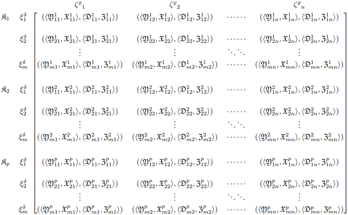
Let $\xi^{\delta} = \{\xi^{\delta}_1, \xi^{\delta}_2, \ldots, \xi^{\delta}_m \} $ be the assemblage of alternatives and $ {\zeta^{\varrho}}= \{{\zeta^{\varrho}}_1, {\zeta^{\varrho}}_2, \ldots, {\zeta^{\varrho}}_n \} $ is the assemblage of criterions, Priorities are assigned between the criteria provided by the linear orientation in this case. ${\zeta^{\varrho}}_1 \succ {\zeta^{\varrho}}_2 \succ {\zeta^{\varrho}}_3 \ldots {\zeta^{\varrho}}_n $ indicates criteria ${\zeta^{\varrho}}_J$ has a high priority than ${\zeta^{\varrho}}_i$ if $j>i$. $ {\tau^{\varsigma}}= \{{\tau^{\varsigma}}_1, {\tau^{\varsigma}}_2, \ldots, {\tau^{\varsigma}}_p \} $ is a assemblage of decision-makers (DMs) and DMs are not given the same priority. Prioritization is provided by a linear pattern between the DMs given as, ${\tau^{\varsigma}}_1 \succ {\tau^{\varsigma}}_2 \succ {\tau^{\varsigma}}_3 \ldots {\tau^{\varsigma}}_p $ shows DM ${\tau^{\varsigma}}_{\zeta}$ has a high imprtance than ${\tau^{\varsigma}}_{\varrho}$ if $\zeta>\varrho$. DMs give a matrix according to their own standpoints $D^{(p)}= ( \mathfrak{B}^{(p)}_{ij})_{m\times n }$, where $ \mathfrak{B}^{(p)}_{ij}$ is given for the alternatives $\xi^{\delta}_i \in \xi^{\delta} $ with respect to the attribute ${\zeta^{\varrho}}_{\gimel} \in {\zeta^{\varrho}}$ by ${\tau^{\varsigma}}_p $ DM. If all Performance criteria are the same kind, there is no need for normalisation; however, since MCGDM has two different types of Evaluation criteria (benefit kind attributes $\tau_b$ and cost kinds attributes $\tau_c$), the matrix $D_(p)$ has been transformed into a normalise matrix using the normalisation formula $Y^{(p)}= (\mathfrak{P}^{(p)}_{ij})_{m\times n }$,
where, $(\mathfrak{B}^{(p)}_{ij})^c $ show the compliment of $\mathfrak{B}^{(p)}_{ij}$.
The suggested operators will be implemented to the MCGDM, which will require the preceding steps.
Algorithm |
Step 1: Acquire a decision matrix $D^{(p)}=\left(\mathfrak{B}_{i j}^{(p)}\right)_{m \times n}$ in the form of LiDFNs from the decision makers. |
 |
Step 2:
Two kinds of criterion are described in the decision matrix: $(\tau_c)$ cost type indicators and $(\tau_b)$ benefit type indicators. There is no need for normalisation if all indicators are of the same kind, but in MCGDM, there may be two types of criteria. The matrix was updated to the transforming response matrix in this case $Y^{(p)}= (\mathfrak{P}^{(p)}_{ij})_{m\times n }$ using the normalization formula Eq. (5).
Step 3:
Calculate the values of ${\aleph^{\hbar}}_{ij}^{(p)}$ by following formula.
Step 4:
Use one of the above mentioned AOs, to get one cumulative matrix $W^{(p)}= (\mathfrak{W}_{ij})_{m\times n }$ by aggregating all LiDF decision matrices $Y^{(p)}= (\mathfrak{P}^{(p)}_{ij})_{m\times n }$.
Step 5:
Values of ${\aleph^{\hbar}}_{ij}$ determine by using given formula.
Step 6:
Aggregate the LiDF values $\mathfrak{W}_{ij}$ for each alternative $\xi^{\delta}_{i}$ by the LiDFSMA (or LiDFSMG) operator:
Step 7:
Compute all cumulative alternative assessments's score.
Step 8:
The alternatives were rated using the score feature, and the best option was chosen.
5. Case Study
The significance of sustainable development and environmental protection in recent years has led to a greater emphasis on green supply chain management. Green supply chain management entails the incorporation of environmental concerns into every aspect of supply chain operations, including procurement, production, distribution, and disposal. The need to maximise efficiency while minimising environmental impact is one of the greatest obstacles organisations face in their pursuit of green supply chain objectives. This paper will examine the significance of improving the efficacy of green supply chains and the role of decision-making in attaining this objective. Green supply chain management relies heavily on efficiency to accomplish its objectives. Several strategies, including the use of renewable energy, the reduction of waste and emissions, and the optimisation of logistics and transportation, can increase the efficiency of green supply chains. Utilization of technology is a significant factor in the efficiency of green supply chains. Technology can assist businesses in optimising their supply chain processes, reducing costs, and minimising environmental impact.
The use of data analytics is one area where technology can have a significant impact on efficiency. Data analytics entails the application of sophisticated algorithms and statistical models to analyse vast datasets and derive actionable insights. In green supply chains, data analytics can be utilised to identify wasteful and inefficient areas and develop strategies to resolve these problems. For instance, data analytics can be used to determine the most cost-effective and environmentally friendly transportation routes and modes, thereby reducing the environmental impact of transportation while minimising costs. Automation is another way in which technology can improve the efficacy of green supply chains. Automation is the use of machines and automata to execute formerly manual tasks. By eliminating errors, reducing cycle times, and increasing throughput, automation can help businesses reduce waste and improve efficiency. For instance, automation can be used to sort and process recyclable materials, thereby reducing the need for manual labour and enhancing sorting precision.
Green supply chain management (GSCM) is a critical approach for achieving sustainability in the supply chain network. It involves the integration of environmental considerations into the supply chain operations to reduce environmental impacts and enhance the economic and social performance of the supply chain. In this essay, we will discuss the criteria for green supply chain management.
One of the most crucial criteria for GSCM is environmental performance. GSCM aims to reduce the environmental impact of supply chain operations, including the reduction of greenhouse gas emissions, water consumption, and waste generation. Companies need to implement environmental management practices such as pollution prevention, waste reduction, energy conservation, and water conservation to improve environmental performance. Another critical criterion for GSCM is supplier management. Companies need to collaborate with their suppliers to ensure that their environmental and social standards are aligned. The supplier selection process should consider the environmental performance of the supplier, including their environmental policies, practices, and certifications. Green procurement is a crucial criterion for GSCM. It involves the purchasing of environmentally friendly products and services. Companies need to develop green procurement policies that consider the environmental impact of products and services, including their life cycle assessment, carbon footprint, and environmental certifications. Stakeholder engagement is another critical criterion for GSCM. It involves the participation of all stakeholders in the supply chain, including customers, suppliers, employees, and local communities. Companies need to engage stakeholders in the decision-making process to ensure that their concerns and perspectives are considered. Compliance with environmental regulations is another critical criterion for GSCM. Companies need to comply with local, national, and international environmental regulations, including laws related to air emissions, water discharge, and waste disposal. Compliance with regulations is essential for protecting the environment and avoiding legal penalties.
Risk management is an essential criterion for GSCM. Companies need to identify and mitigate environmental risks in their supply chain operations. They need to develop risk management plans that consider potential environmental risks, including natural disasters, climate change, and resource scarcity. Life cycle assessment (LCA) is a critical criterion for GSCM. It involves the evaluation of the environmental impacts of a product or service throughout its life cycle, from raw material extraction to end-of-life disposal. Companies need to conduct LCA to identify opportunities for environmental improvement and make informed decisions regarding product design, sourcing, and disposal. Green logistics is a critical criterion for GSCM. It involves the optimization of logistics operations to reduce the environmental impact of transportation, warehousing, and distribution activities. Companies need to implement green logistics practices such as route optimization, fuel-efficient transportation, and use of alternative transportation modes. Performance measurement and reporting are essential criteria for GSCM. Companies need to measure and report their environmental performance regularly to track their progress towards sustainability goals. Performance indicators should include environmental metrics such as greenhouse gas emissions, water consumption, and waste generation. Continuous improvement is a critical criterion for GSCM. Companies need to continuously improve their environmental performance by implementing new environmental management practices and technologies. Continuous improvement involves the development of an environmental management system that enables companies to monitor and evaluate their environmental performance regularly.
GSCM has the potential to significantly impact the economy of a country. By implementing GSCM practices, businesses can reduce their environmental impact while also increasing their efficiency and profitability. This can lead to several economic benefits for the country as a whole. One key economic benefit of GSCM is cost savings. GSCM practices can help businesses reduce their costs by identifying areas of inefficiency and waste in their supply chain. For example, reducing energy consumption and water usage can lead to lower utility bills. Similarly, reducing waste generation can reduce disposal costs. These cost savings can help businesses increase their profitability, which in turn can stimulate economic growth. Another economic benefit of GSCM is increased competitiveness. As more and more businesses adopt GSCM practices, those that fail to do so risk falling behind. By implementing GSCM practices, businesses can differentiate themselves from their competitors and appeal to consumers who are increasingly environmentally conscious. This can help businesses increase their market share and drive economic growth.
GSCM can also lead to increased revenue streams. For example, businesses can develop new products or services that are environmentally friendly, which can appeal to a growing market of consumers who prioritize sustainability. Similarly, businesses can market their environmental initiatives to attract new customers and retain existing ones. By tapping into these new revenue streams, businesses can increase their profitability and contribute to economic growth. In addition to these direct economic benefits, GSCM can also have indirect economic benefits. For example, GSCM can help businesses build strong relationships with their suppliers, customers, and other stakeholders. This can lead to increased collaboration and knowledge-sharing, which can drive innovation and improve the overall efficiency of the supply chain. This increased efficiency can benefit the economy as a whole by reducing costs and improving productivity. Furthermore, GSCM can help businesses comply with environmental regulations, which can reduce the risk of fines and legal action. This can help businesses avoid costly legal battles and maintain their reputation, which can in turn increase their profitability and competitiveness. However, there are also potential challenges associated with implementing GSCM practices. For example, there may be a higher upfront cost associated with investing in new technologies or equipment to reduce environmental impact. Additionally, implementing GSCM practices may require significant changes to the organization's culture and processes, which can be challenging to manage. Finally, there may be a lack of understanding or awareness among stakeholders about the benefits of GSCM, which can make it difficult to gain buy-in and support for these initiatives.
Consider a set of alternatives $\xi^{\delta} = \{\xi^{\delta}_1, \xi^{\delta}_2, \xi^{\delta}_3, \xi^{\delta}_4 \} $ and ${\zeta^{\varrho}}= \{{\zeta^{\varrho}}_1, {\zeta^{\varrho}}_2, {\zeta^{\varrho}}_3, {\zeta^{\varrho}}_4, {\zeta^{\varrho}}_5, \} $ is the finite set of criterions, where ${\zeta^{\varrho}}_1$= cost, ${\zeta^{\varrho}}_2$=reputation, ${\zeta^{\varrho}}_3$=innovation in services, ${\zeta^{\varrho}}_4$=environment friendly, ${\zeta^{\varrho}}_5$=geographical specialization and ${\zeta^{\varrho}}_6$=financial condition, Priorities are assigned between the criteria provided by the linear orientation in this case. ${\zeta^{\varrho}}_1 \succ {\zeta^{\varrho}}_2 \succ {\zeta^{\varrho}}_3 \ldots {\zeta^{\varrho}}_6 $ indicates criteria ${\zeta^{\varrho}}_J$ has a high priority than ${\zeta^{\varrho}}_i$ if $j>i$. In this example we use LiDFNs as input data for ranking the given alternatives under the given attributes. Here three DMs are involved i.e ${\tau^{\varsigma}}_1, {\tau^{\varsigma}}_2$ and ${\tau^{\varsigma}}_3$. DMs are not given the same priority. Prioritization is provided by a linear pattern between the DMs given as, ${\tau^{\varsigma}}_1 \succ {\tau^{\varsigma}}_2 \succ {\tau^{\varsigma}}_3 $ shows DM ${\tau^{\varsigma}}_{\zeta}$ has a high imprtance than ${\tau^{\varsigma}}_{\varrho}$ if $\zeta>\varrho$.
Step 1:
Compute the decision matrix $D^{(p)}= ( \mathfrak{B}^{(p)}_{ij})_{m\times n }$ in the form of LiDFNs, given in Table 1, Table 2 and Table 3.
| $\zeta_1^{\varrho}$ | $\zeta_2^\rho$ | $\zeta_3^{\varrho}$ | $\zeta_4^\rho$ | $\zeta_5^\rho$ |
$\xi_1^\delta$ | (⟨0.21, 0.86⟩, ⟨0.16, 0.66⟩) | (⟨0.96, 0.56⟩, ⟨0.46, 0.16⟩) | (⟨0.86, 0.11⟩, ⟨0.51, 0.11⟩) | (⟨0.46, 0.26⟩, ⟨0.61, 0.11⟩) | (⟨0.86, 0.21⟩, ⟨0.81, 0.11⟩) |
$\xi_2^\delta$ | (⟨0.11, 0.41⟩, ⟨0.26, 0.36⟩) | (⟨0.61, 0.46⟩, ⟨0.66, 0.16⟩) | (⟨0.66, 0.16⟩, ⟨0.31, 0.31⟩) | (⟨0.56, 0.36⟩, ⟨0.41, 0.36⟩) | (⟨0.66, 0.11⟩, ⟨0.16, 0.26⟩) |
$\xi_3^\delta$ | (⟨0.21, 0.66⟩, ⟨0.36, 0.16⟩) | (⟨0.41, 0.51⟩, ⟨0.31, 0.41⟩) | (⟨0.51, 0.21⟩, ⟨0.46, 0.46⟩) | (⟨0.66, 0.46⟩, ⟨0.26, 0.26⟩) | (⟨0.41, 0.61⟩, ⟨0.30, 0.30⟩) |
$\xi_4^\delta$ | (⟨0.30, 0.50⟩, ⟨0.16, 0.60⟩) | (⟨0.60, 0.56⟩, ⟨0.16, 0.16⟩) | (⟨0.66, 0.36⟩, ⟨0.20, 0.30⟩) | (⟨0.86, 0.16⟩, ⟨0.40, 0.40⟩) | (⟨0.86, 0.96⟩, ⟨0.10, 0.30⟩) |
| $\zeta_1^{\varrho}$ | $\zeta_2^\rho$ | $\zeta_3^{\varrho}$ | $\zeta_4^\rho$ | $\zeta_5^\rho$ |
$\xi_1^\delta$ | (⟨0.86, 0.46⟩, ⟨0.40, 0.36⟩) | (⟨0.86, 0.46⟩, ⟨0.26, 0.46⟩) | (⟨0.96, 0.86⟩, ⟨0.36, 0.66⟩) | (⟨0.46, 0.26⟩, ⟨0.80, 0.66⟩) | (⟨0.40, 0.26⟩, ⟨0.46, 0.26⟩) |
$\xi_2^\delta$ | (⟨0.66, 0.36⟩, ⟨0.30, 0.46⟩) | (⟨0.66, 0.50⟩, ⟨0.36, 0.26⟩) | (⟨0.40, 0.30⟩, ⟨0.36, 0.56⟩) | (⟨0.66, 0.36⟩, ⟨0.26, 0.36⟩) | (⟨0.50, 0.66⟩, ⟨0.36, 0.20⟩) |
$\xi_3^\delta$ | (⟨0.26, 0.46⟩, ⟨0.30, 0.30⟩) | (⟨0.46, 0.96⟩, ⟨0.26, 0.46⟩) | (⟨0.66, 0.26⟩, ⟨0.36, 0.26⟩) | (⟨0.46, 0.46⟩, ⟨0.46, 0.26⟩) | (⟨0.60, 0.36⟩, ⟨0.66, 0.16⟩) |
$\xi_4^\delta$ | (⟨0.86, 0.60⟩, ⟨0.20, 0.46⟩) | (⟨0.66, 0.40⟩, ⟨0.30, 0.66⟩) | (⟨0.36, 0.66⟩, ⟨0.46, 0.46⟩) | (⟨0.30, 0.86⟩, ⟨0.30, 0.40⟩) | (⟨0.30, 0.40⟩, ⟨0.26, 0.46⟩) |
Step 2:
Normalize the decision matrixes using Eq. (5). First criteria is ${\zeta^{\varrho}}_1$ cost type and other is benefit type, given in Table 4, Table 5 and Table 6.
| $\zeta_1^{\varrho}$ | $\zeta_2^\rho$ | $\zeta_3^{\varrho}$ | $\zeta_4^\rho$ | $\zeta_5^\rho$ |
$\xi_1^\delta$ | (⟨0.46, 0.36⟩, ⟨0.46, 0.30⟩) | (⟨0.66, 0.26⟩, ⟨0.66, 0.20⟩) | (⟨0.66, 0.20⟩, ⟨036., 0.16⟩) | (⟨0.86, 0.16⟩, ⟨0.30, 0.30⟩) | (⟨0.66, 0.16⟩, ⟨0.36, 0.26⟩) |
$\xi_2^\delta$ | (⟨0.26, 0.45⟩, ⟨0.30, 0.30⟩) | (⟨0.46, 0.26⟩, ⟨0.20, 0.36⟩) | (⟨0.36, 0.16⟩, ⟨0.66, 0.20⟩) | (⟨0.26, 0.66⟩, ⟨0.40, 0.40⟩) | (⟨0.60, 0.46⟩, ⟨0.20, 0.30⟩) |
$\xi_3^\delta$ | (⟨0.86, 0.60⟩, ⟨0.20, 0.46⟩) | (⟨0.60, 0.80⟩, ⟨0.60, 0.30⟩) | (⟨0.26, 0.60⟩, ⟨0.36, 0.40⟩) | (⟨0.36, 0.90⟩, ⟨0.26, 0.10⟩) | (⟨0.60, 0.86⟩, ⟨0.46, 0.46⟩) |
$\xi_4^\delta$ | (⟨0.40, 0.66⟩, ⟨0.16, 0.36⟩) | (⟨0.46, 0.40⟩, ⟨0.26, 0.46⟩) | (⟨0.16, 0.46⟩, ⟨0.30, 0.30⟩) | (⟨0.40, 0.60⟩, ⟨0.20, 0.60⟩) | (⟨0.40, 0.36⟩, ⟨0.60, 0.20⟩) |
| $\zeta_1^{\varrho}$ | $\zeta_2^\rho$ | $\zeta_3^{\varrho}$ | $\zeta_4^\rho$ | $\zeta_5^\rho$ |
$\xi_1^\delta$ | (⟨0.86, 0.21⟩, ⟨0.66, 0.16⟩) | (⟨0.96, 0.56⟩, ⟨0.46, 0.16⟩) | (⟨0.86, 0.11⟩, ⟨0.51, 0.11⟩) | (⟨0.46, 0.26⟩, ⟨0.61, 0.11⟩) | (⟨0.86, 0.21⟩, ⟨0.81, 0.11⟩) |
$\xi_2^\delta$ | (⟨0.41, 0.11⟩, ⟨0.36, 0.26⟩) | (⟨0.61, 0.46⟩, ⟨0.66, 0.16⟩) | (⟨0.66, 0.16⟩, ⟨0.31, 0.31⟩) | (⟨0.56, 0.36⟩, ⟨0.41, 0.36⟩) | (⟨0.66, 0.11⟩, ⟨0.16, 0.26⟩) |
$\xi_3^\delta$ | (⟨0.66, 0.21⟩, ⟨0.16, 0.36⟩) | (⟨0.41, 0.51⟩, ⟨0.31, 0.41⟩) | (⟨0.51, 0.21⟩, ⟨0.46, 0.46⟩) | (⟨0.66, 0.46⟩, ⟨0.26, 0.26⟩) | (⟨0.41, 0.61⟩, ⟨0.30, 0.30⟩) |
$\xi_4^\delta$ | (⟨0.50, 0.30⟩, ⟨0.60, 0.16⟩) | (⟨0.60, 0.56⟩, ⟨0.16, 0.16⟩) | (⟨0.66, 0.36⟩, ⟨0.20, 0.30⟩) | (⟨0.86, 0.16⟩, ⟨0.40, 0.40⟩) | (⟨0.86, 0.96⟩, ⟨0.10, 0.30⟩) |
| $\zeta_1^{\varrho}$ | $\zeta_2^\rho$ | $\zeta_3^{\varrho}$ | $\zeta_4^\rho$ | $\zeta_5^\rho$ |
$\xi_1^\delta$ | (⟨0.46, 0.86⟩, ⟨0.36, 0.40⟩) | (⟨0.86, 0.46⟩, ⟨0.26, 0.46⟩) | (⟨0.96, 0.86⟩, ⟨0.36, 0.66⟩) | (⟨0.46, 0.26⟩, ⟨0.80, 0.66⟩) | (⟨0.40, 0.26⟩, ⟨0.46, 0.26⟩) |
$\xi_2^\delta$ | (⟨0.36, 0.66⟩, ⟨0.46, 0.30⟩) | (⟨0.66, 0.50⟩, ⟨0.36, 0.26⟩) | (⟨0.40, 0.30⟩, ⟨0.36, 0.56⟩) | (⟨0.66, 0.36⟩, ⟨0.26, 0.36⟩) | (⟨0.50, 0.66⟩, ⟨0.36, 0.20⟩) |
$\xi_3^\delta$ | (⟨0.46, 0.26⟩, ⟨0.30, 0.30⟩) | (⟨0.46, 0.96⟩, ⟨0.26, 0.46⟩) | (⟨0.66, 0.26⟩, ⟨0.36, 0.26⟩) | (⟨0.46, 0.46⟩, ⟨0.46, 0.26⟩) | (⟨0.60, 0.36⟩, ⟨0.66, 0.16⟩) |
$\xi_4^\delta$ | (⟨0.60, 0.86⟩, ⟨0.46, 0.20⟩) | (⟨0.66, 0.40⟩, ⟨0.30, 0.66⟩) | (⟨0.36, 0.66⟩, ⟨0.46, 0.46⟩) | (⟨0.30, 0.86⟩, ⟨0.30, 0.40⟩) | (⟨0.30, 0.40⟩, ⟨0.26, 0.46⟩) |
| $\zeta_1^{\varrho}$ | $\zeta_2^\rho$ | $\zeta_3^{\varrho}$ | $\zeta_4^\rho$ | $\zeta_5^\rho$ |
$\xi_1^\delta$ | (⟨0.36, 0.46⟩, ⟨0.30, 0.46⟩) | (⟨0.66, 0.26⟩, ⟨0.66, 0.20⟩) | (⟨0.66, 0.20⟩, ⟨036., 0.16⟩) | (⟨0.86, 0.16⟩, ⟨0.30, 0.30⟩) | (⟨0.66, 0.16⟩, ⟨0.36, 0.26⟩) |
$\xi_2^\delta$ | (⟨0.45, 0.26⟩, ⟨0.30, 0.30⟩) | (⟨0.46, 0.26⟩, ⟨0.20, 0.36⟩) | (⟨0.36, 0.16⟩, ⟨0.66, 0.20⟩) | (⟨0.26, 0.66⟩, ⟨0.40, 0.40⟩) | (⟨0.60, 0.46⟩, ⟨0.20, 0.30⟩) |
$\xi_3^\delta$ | (⟨0.60, 0.86⟩, ⟨0.46, 0.20⟩) | (⟨0.60, 0.80⟩, ⟨0.60, 0.30⟩) | (⟨0.26, 0.60⟩, ⟨0.36, 0.40⟩) | (⟨0.36, 0.90⟩, ⟨0.26, 0.10⟩) | (⟨0.60, 0.86⟩, ⟨0.46, 0.46⟩) |
$\xi_4^\delta$ | (⟨0.66, 0.40⟩, ⟨0.36, 0.16⟩) | (⟨0.46, 0.40⟩, ⟨0.26, 0.46⟩) | (⟨0.16, 0.46⟩, ⟨0.30, 0.30⟩) | (⟨0.40, 0.60⟩, ⟨0.20, 0.60⟩) | (⟨0.40, 0.36⟩, ⟨0.60, 0.20⟩) |
Step 3:
Calculate the values of $\breve{\hbar}_{i j}^{(p)}$ by Eq. (6).
$\breve{\hbar}_{i j}^{(1)}=\left(\begin{array}{lllll}1 & 1 & 1 & 1 & 1 \\ 1 & 1 & 1 & 1 & 1 \\ 1 & 1 & 1 & 1 & 1 \\ 1 & 1 & 1 & 1 & 1\end{array}\right)$
$\breve{\hbar}_{i j}^{(2)}=\left(\begin{array}{ccccc}0.7876 & 0.7600 & 0.7876 & 0.7600 & 0.8176 \\ 0.6760 & 0.6646 & 0.6460 & 0.6646 & 0.6146 \\ 0.6646 & 0.6460 & 0.6760 & 0.6600 & 0.6176 \\ 0.6646 & 0.6146 & 0.6600 & 0.6760 & 0.4460\end{array}\right)$
$\breve{\hbar}_{i j}^{(3)}=\left(\begin{array}{lllll}0.1064 & 0.1461 & 0.1644 & 0.4969 & 0.6648 \\ 0.1144 & 0.1747 & 0.1418 & 0.1094 & 0.1061 \\ 0.1616 & 0.4100 & 0.1694 & 0.4611 & 0.1696 \\ 0.1111 & 0.4060 & 0.4118 & 0.4478 & 0.1488\end{array}\right)$
Step 4:
Use LiDFPWA to aggregate all individual LiDF decision matrices $Y^{(p)}=\left(\mathfrak{P}_{i j}^{(p)}\right)_{m \times n}$ into one cumulative assessments matrix of the alternatives $W^{(p)}=\left(\mathfrak{W}_{i j}\right)_{m \times n}$, given below
$\left.\begin{array}{cccc} & \zeta^{\varrho}{ }_1 & \zeta^{\varrho}{ }_2 & \zeta^{\varrho}{ }_3 \\ \xi_1^\delta & (\langle 0.6661,0.4180\rangle,\langle 0.4113,0.3446\rangle) & (\langle 0.8660,0.4434\rangle,\langle 0.6080,0.3416\rangle) & (\langle 0.8848,0.3463\rangle,\langle 0.4340,0.3138\rangle) \\ \xi_2^\delta & (\langle 0.6306,0.3181\rangle,\langle 0.3686,0.3636\rangle) & (\langle 0.6486,0.4183\rangle,\langle 0.4016,0.3066\rangle) & (\langle 0.6386,0.1866\rangle,\langle 0.3643,0.3388\rangle) \\ \xi_3^\delta & (\langle 0.6641,0.3686\rangle,\langle 0.3488,0.3018\rangle) & (\langle 0.6441,0.6346\rangle,\langle 0.3438,0.3616\rangle) & (\langle 0.4141,0.3631\rangle,\langle 0.4036,0.3666\rangle)) \\ \xi_4^\delta & (\langle 0.4634,0.4881\rangle,\langle 0.4180,0.1640\rangle) & (\langle 0.6006,0.6083\rangle,\langle 0.3066,0.3646\rangle) & (\langle 0.4343,0.4680\rangle,\langle 0.3666,0.3368\rangle)\end{array}\right)$
$\left.\begin{array}{ccc} & \zeta^{\varrho}{ }_4 & \zeta^{\varrho}{ }_5 \\ \xi_1^\delta & (\langle 0.6666,0.3333\rangle,\langle 0.6408,0.3381\rangle) & (\langle 0.6646,0.3066\rangle,\langle 0.6886,0.1466\rangle) \\ \xi_3^\delta & (\langle 0.4460,0.3866\rangle,\langle 0.3484,0.3468\rangle) & (\langle 0.4663,0.3406\rangle,\langle 0.3363,0.3366\rangle) \\ \xi_3^\delta & (\langle 0.4610,0.4808\rangle,\langle 0.3164,0.3160\rangle) & (\langle 0.6636,0.4414\rangle,\langle 0.4406,0.3666\rangle) \\ \xi_4^\delta & (\langle 0.6641,0.3366\rangle,\langle 0.3440,0.4106\rangle) & (\langle 0.6408,0.6661\rangle,\langle 0.1864,0.3333\rangle)\end{array}\right)$
Step 5:
Evaluate the values of $\breve{\hbar}_{i j}$ by using Eq. (7).
$\breve{\hbar}_{i j}=\left(\begin{array}{lllll}1 & 0.3333 & 0.4314 & 0.3074 & 0.2272 \\ 1 & 0.3233 & 0.3338 & 0.2471 & 0.1334 \\ 1 & 0.3884 & 0.3073 & 0.1733 & 0.0314 \\ 1 & 0.3038 & 0.2333 & 0.1481 & 0.0832\end{array}\right)$
Step 6:
Aggregate the LiDF values $\mathfrak{W}_{i j}$ for each alternative $\xi_i^\delta$ by the LiDFPWA operator using Eq. (2) given in Table 7.
$\mathfrak{W}_1$ | (⟨0.7150, 0.3564⟩, ⟨0.5229, 0.2218⟩) |
$\mathfrak{W}_2$ | (⟨0.2454, 0.2794⟩, ⟨0.4269, 0.2319⟩) |
$\mathfrak{W}_3$ | (⟨0.6296, 0.3477⟩, ⟨0.3181, 0.3313⟩) |
$\mathfrak{W}_4$ | (⟨0.5185, 0.5325⟩, ⟨0.3408, 0.2352⟩) |
Step 7:
Calculate the score of all LiDF aggregated values $\mathfrak{W}_i$.
$\begin{aligned} \mathfrak{H}\left(\mathfrak{W}_1\right) & =0.6969 \\ \mathfrak{H}\left(\mathfrak{W}_2\right) & =0.6259 \\ \mathfrak{H}\left(\mathfrak{W}_3\right) & =0.5735 \\ \mathfrak{H}\left(\mathfrak{W}_4\right) & =0.5595\end{aligned}$
Step 8:
Rank by score function values.
$\mathfrak{W}_1 \succ \mathfrak{W}_2 \succ \mathfrak{W}_3 \succ \mathfrak{W}_4$
So,
$\xi_1^\delta \succ \xi_2^\delta \succ \xi_3^\delta \succ \xi_4^\delta$
6. Conclusion
Green supply chain management is crucial for waste reduction, optimizing resources, and minimizing the environmental impact of operations. A comprehensive strategy covering the entire supply chain, from product design to transportation, is necessary to implement sustainable practices. By doing so, businesses can improve their environmental performance, reduce costs, enhance customer satisfaction, and gain a competitive edge in the market. However, selecting the optimal green provider is a complex and challenging decision-making issue due to competing characteristics, uncertainties in the physical universe, and a lack of knowledge. To address this, we introduced novel aggregation operators within a linear-diophantine fuzzy (LiDF) framework, such as the linear Diophantine fuzzy soft-max average (LiDFSMA) operator and the linear Diophantine fuzzy soft-max geometric (LiDFSMG) operator. The proposed method was validated using a simple example of a green supplier optimization technique with linear Diophantine fuzzy content, showcasing the utility and applicability of the proposed method in aiding decision-makers in selecting the optimal course of action.
The introduction of novel aggregation operators can increase the effectiveness of green supply chains by allowing decision-makers to choose the best alternative. In conclusion, the proposed method provides a potential means of improving the efficacy of green supply chains.
The data used to support the findings of this study are available from the corresponding author upon request.
The authors declare that they have no conflicts of interest.