the Creative Commons Attribution 4.0 License.
the Creative Commons Attribution 4.0 License.
 | 14 Mar 2024
An insight into the capability of the actuator line method to resolve tip vortices
Pier Francesco Melani
Omar Sherif Mohamed
Stefano Cioni
Francesco Balduzzi
Alessandro Bianchini
The actuator line method (ALM) is increasingly being preferred to the ubiquitous blade element momentum (BEM) approach in several applications related to wind turbine simulation, thanks to the higher level of fidelity required by the design and analysis of modern machines. Its capability to resolve blade tip vortices and their effect on the blade load profile is, however, still unsatisfactory, especially when compared to other medium-fidelity methodologies such as the lifting line theory (LLT). Despite the numerical strategies proposed so far to overcome this limitation, the reason for such behavior is still unclear. To investigate this aspect, the present study uses the ALM tool developed by the authors for the ANSYS® Fluent® solver (v. 20.2) to simulate a NACA0018 finite wing for different pitch angles. Three different test cases were considered: high-fidelity blade-resolved computational fluid dynamics (CFD) simulations (to be used as a benchmark), standard ALM, and ALM with the spanwise force distribution coming from blade-resolved data (frozen ALM). The last option was included to isolate the effect of force projection, using three different smearing functions. For the postprocessing of the results, two different techniques were applied: the LineAverage sampling of the local angle of attack along the blade and state-of-the-art vortex identification methods (VIMs) to outline the blade vortex system. The analysis showed that the ALM can account for tip effects without the need for additional corrections, provided that the correct angle of attack sampling and force projection strategies are adopted.
- Article
(10053 KB) - Full-text XML
- BibTeX
- EndNote


1.1 Background and motivation
The actuator line method (ALM) (Sørensen and Shen, 2002), i.e., the replacement of rotor blades with dynamically equivalent actuator lines inside a computational fluid dynamics (CFD) domain, is increasingly being preferred in wind turbine simulations to the widely used blade element momentum (BEM) approach. This holds true particularly in modern, large, and highly flexible turbines (Veers et al., 2023) due to the higher level of fidelity required for their aeroelastic design and analysis (Boorsma et al., 2020; Perez-Becker et al., 2020). In fact, as the size of their rotors is progressively becoming larger and larger, the study of horizontal-axis wind turbines (HAWTs) needs tools capable of resolving the interaction between the increasingly deformable blades and the turbulent structures generated in the atmosphere at the micro- and mesoscale level, as well as in the wake of neighboring turbines (Veers et al., 2019). In addition, another area in which ALM is receiving attention is connected to the renewed interest in vertical-axis wind turbines (VAWTs) for deep-sea, floating offshore installations (Cooper, 2010); the inherently unsteady aerodynamics of these machines (Ferreira et al., 2007), connected to the continuous variation in angle of attack, make the use of blade-resolved simulations prohibitive, paving the way for the use of a method like ALM. However, there is still a gap between this and other medium-fidelity approaches used for rotor simulation, such as lifting line theory (LLT) (Marten et al., 2015) or vortex-based panel methods (Greco and Testa, 2021), in terms of accuracy in the resolution of the blade tip vortices and their effect on the blade loads (Balduzzi et al., 2018; Boorsma et al., 2023). This issue becomes critical when simulating high-load conditions, such as high tip-speed ratios (TSRs) in VAWTs, since the ALM largely overestimates the rotor power production (Melani et al., 2021b).
Upon examination of the literature, the scientific community seems to agree that the reason for this behavior lies in the tendency of the ALM to “overspread” the computed aerodynamic forces into the domain. The resolved tip vortex structure and the corresponding downwash along the blade are therefore underestimated. Shives and Crawford (2013) conducted the first systematic investigation on the influence of the kernel width β and relative cell size on the predicted blade loads (Shives and Crawford, 2013). Their study revealed that, for a fixed-wing case, the parameter β should be scaled as a fraction of the chord length, c. They demonstrated that a ratio around 0.25 is required to successfully simulate the tip vortex system within the ALM framework. To maintain an accurate estimation of the local angle of attack, which was sampled along the actuator line, they also imposed a constraint on the element size in the cell zone where the blade forces are inserted (hALM), which needs to be lower than 0.25 β; 3 years later, Martínez-Tossas et al. (2016), Jha et al. (2014), and Jha and Schmitz (2018) proved that the findings of Shives and Crawford (2013) also apply to the simulation of horizontal-axis wind turbines (HAWTs). Jha et al. (2014) also proposed the reduction of β/c towards the tip according to an elliptical law, suggesting this would improve the prediction of the blade circulation distribution. Taking the concept even further, Churchfield et al. (2017) replaced the standard isotropic Gaussian smearing function with an arbitrary one, which can be shaped according to the actual geometry of the rotor blade. Although effective, the two methodologies require case-specific tuning and finer grids than the standard ALM, since the mesh in the rotor region needs to be refined to accommodate the resolution adopted at the blade tip. Although extensive and innovative for the time, the studies described so far are not exempt from limitations, in particular (a) the lack of proper validation data, usually replaced by analytical solutions or simulations done with low-order methods like BEM; (b) the lack of insight into the physical/numerical mechanisms involved, as most analyses focused on integral quantities like the blade torque; and (c) the complexity of the selected test cases. Point (c) refers to the studies on horizontal-axis rotors, where the effect of blade tapering makes it more complicated to isolate the effect of trailing vorticity on the blade loads.
Recent studies from the National Renewable Energy Laboratory (NREL) (Martínez-Tossas and Meneveau, 2019) and Danmarks Tekniske Universitet (DTU) (Dağ and Sørensen, 2020; Meyer Forsting et al., 2019) took a different direction, focusing on computational efficiency rather than the accuracy of the ALM in describing the blade vortex system and its effects on the loads. The solution proposed by both institutes is a hybrid model, which corrects the over-diffusion of aerodynamic forces typical of the ALM by estimating via LLT the contribution to the downwash induced by tip vortices that is dissipated in the smearing of the blade forces. Although effective and robust, as also demonstrated by some of the authors in a recent publication (Melani et al., 2022), this approach has the major flaw that the induction coming from the vortices already shed in the wake must be accounted for with some sort of wake model. If this is feasible for horizontal-axis machines, at least in simple cases, it becomes almost impossible for vertical-axis ones, where the tip vortices from different blades interact with each other downstream of the turbine (Dossena et al., 2015). Therefore, the potential of the ALM method is not fully exploited.
1.2 Scope of the study
From this perspective, this study aims at extensively investigating the ALM's capability to simulate tip effects, using the ALM tool developed by the authors for the ANSYS® Fluent® solver (v. 20.2) (Melani et al., 2021b). The object of the analysis is a NACA0018 finite wing, under different pitch angles. Three different test cases are considered: high-fidelity blade-resolved CFD (BR-CFD) simulations, to be used as a benchmark; ALM without any correction (standard ALM); and ALM with the spanwise force distribution extracted from blade-resolved data (frozen ALM). The last option is included to isolate the contribution of the adopted force projection strategy, using both isotropic and anisotropic Gaussian smearing functions.
For comparison of the three cases, two different families of postprocessing techniques are applied. On one hand, the blade spanwise flow field is analyzed via the LineAverage technique for the sampling of the local angle of attack (Jost et al., 2018), recently validated by some of the authors in previous work (Melani et al., 2020). In the analysis of BR-CFD results, this approach is supported by the angle of attack reconstruction technique from Soto-Valle et al. (2020, 2021), which is based on the analysis of the blade pressure coefficient distribution. On the other hand, the most recent vortex identification methods (VIMs) from the literature (van der Wall and Richard, 2006; Soto-Valle et al., 2022) are adopted to outline the structure and decay of the tip vortex.
In the present study, the ALM formulation from Melani et al. (2021b) is utilized. The code is implemented within the ANSYS® Fluent® solver (v. 20.2), using a user-defined function (UDF). In the ALM, the blade geometry is not directly resolved but modeled using a lumped-parameter approach, resulting in a significant computational cost reduction. The flow field across the wing is resolved using CFD. The corresponding algorithm for each blade element could be described as follows: firstly, the local flow field is sampled to compute the section relative velocity and angle of attack, which are then used to obtain the corresponding lift, drag, and pitching moment coefficients from tabulated polar data. Finally, the forces are exerted as sources of momentum into the CFD domain via a Gaussian function also known as regularization kernel. For the sampling of the angle of attack, the code uses the novel LineAverage technique (Melani et al., 2021b). Originally derived from Jost et al. (2018), this method calculates the undisturbed velocity V as the integral average of the flow velocity field along a circular sampling line (see Eq. 9). The line is centered at the airfoil quarter chord and has a radius rs=1 c.
In this study, a variation in the ALM called the frozen ALM is utilized alongside the standard ALM. Unlike the conventional ALM, the frozen ALM directly obtains the airfoil aerodynamic forces from a blade-resolved CFD simulation. As rotor loads are not a solver variable anymore, there is no need to iterate between the force computation and flow field resolution steps. Bypassing the use of tabulated data, the frozen ALM effectively eliminates uncertainties associated with the quality of airfoil polar data and the ad hoc correction models that are typically employed. The frozen ALM was initially introduced by Martínez-Tossas et al. (2017) and has previously been employed by the authors in their recent work (Mohamed et al., 2022) to investigate the limitations and challenges of the ALM specifically for vertical-axis turbines. Building upon this prior research, the present study applies the frozen ALM for the first time in a 3D flow regime. By extending the application of the frozen ALM to this flow regime, the study aims to get a better understanding of the capabilities and potential of the ALM in accurately representing the complex flow phenomena connected to tip vortices.
2.1 Regularization kernel
For the regularization kernel, three distinct Gaussian functions, shown in Fig. 1, are utilized:
-
Isotropic Gaussian (Shives and Crawford, 2013), where the forces are equally distributed in the chord and thickness direction within a cylindrical shape. The expression for this function is as follows:
-
Anisotropic Gaussian (Churchfield et al., 2017), a 2D distribution, wherein forces are distributed in an elliptical shape using distinct kernel widths in the chord and thickness directions, denoted as βc and βt, respectively. The expression for this function is
-
Anisotropic Gaussian–Gumbel (Schollenberger et al., 2020), akin to the anisotropic Gaussian but with an incorporated Gumbel function in the chordwise direction, mimicking the airfoil shape. The expression for this function is
In Eqs. (1)–(3), r denotes the distance between the centroid of the generic cell and the actuator line, while β represents the kernel width parameter, which is associated with a characteristic dimension of the airfoil (e.g., chord c), as described in Shives and Crawford (2013). To evaluate the anisotropic kernel functions, r and β are split into their components along the thickness-wise (subscript t) and chordwise (subscript c) directions, as shown in Fig. 1. For the isotropic Gaussian, β is set to 0.1 c, while for both the anisotropic Gaussian and anisotropic Gaussian–Gumbel, a setup with βc=0.2 c and βt=0.1 c is defined. These specific values are selected based on the calibration analysis conducted by the authors in Mohamed et al. (2022) for a 2D airfoil. For more comprehensive information about the ALM code, refer to Melani et al. (2021b).
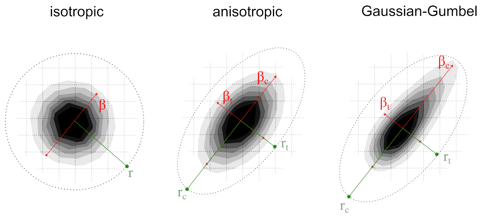
Figure 1Schematic representation of the three different kernel functions used for the ALM simulations in the present work.
2.2 Numerical setup
ALM simulations are carried out with the steady Reynolds-averaged Navier–Stokes (RANS) CFD solver available in Ansys® Fluent® (v. 20.2). The corresponding setup follows a consolidated numerical approach developed by some of the authors for airfoil simulation (Balduzzi et al., 2021), which features the coupled algorithm for pressure–velocity coupling and the second-order upwind scheme for both RANS and turbulence equations. The k–ω shear stress transport (SST) is used for turbulence modeling.
Figures 2a and 3a illustrate the adopted computational domain, whose dimensions – length L=60 c, width W=40 c, and height HD=3 H – are selected to minimize blockage effects and allow the blade wake to develop properly. At the boundaries, the standard far-field boundary conditions for external flows are applied: uniform velocity at the inlet, ambient pressure at the outlet, and symmetry on the other surfaces (including the bottom one). This way, the spanwise symmetry of the problem is exploited, thus halving the global number of elements.
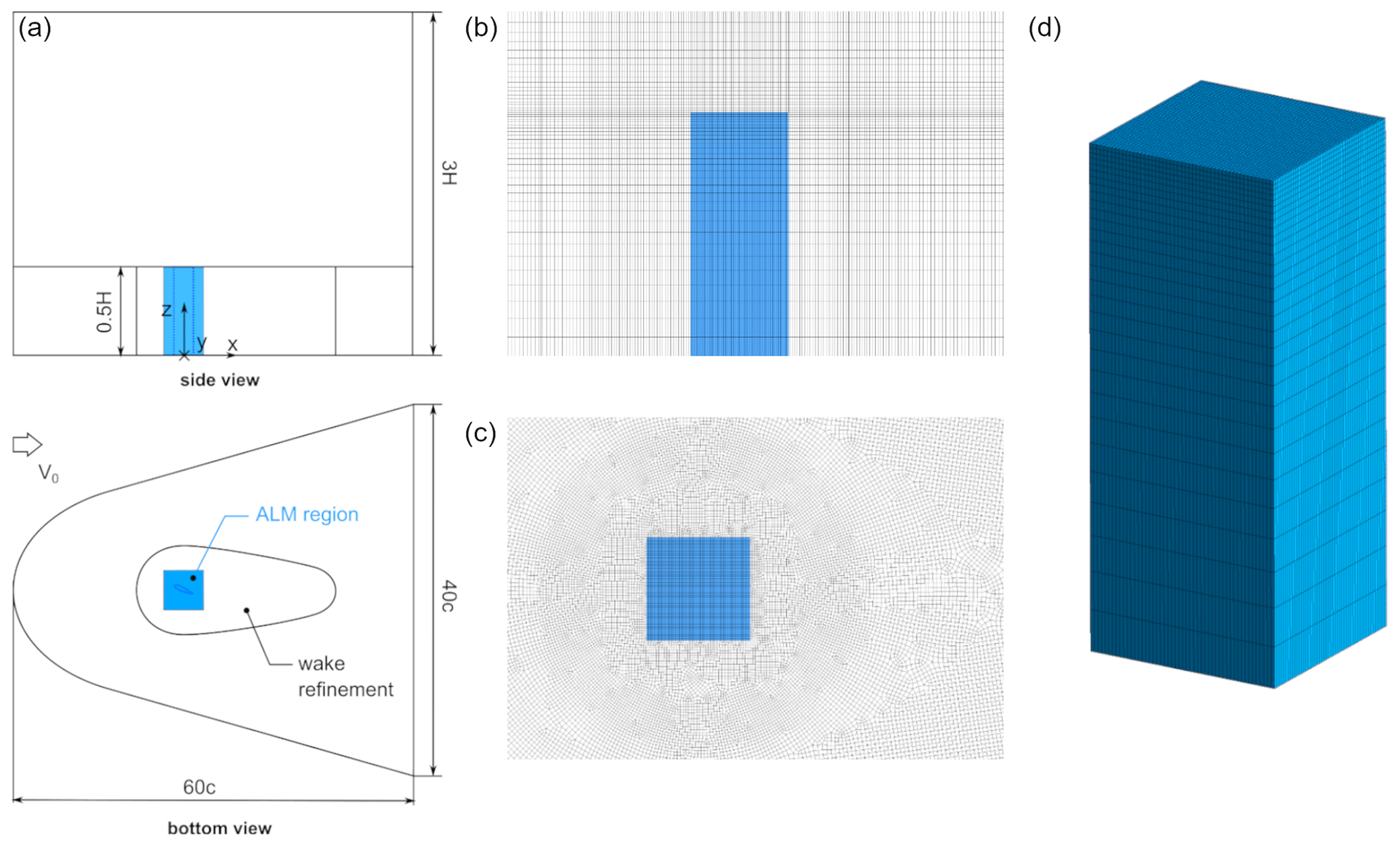
Figure 2Overview of the grid used for ALM simulations: (a) computational domain, (b) side view of the mesh corresponding to the wing, (c) detail of the ALM region at the wing midspan, and (d) detail of the surface mesh along the ALM region in the spanwise direction.
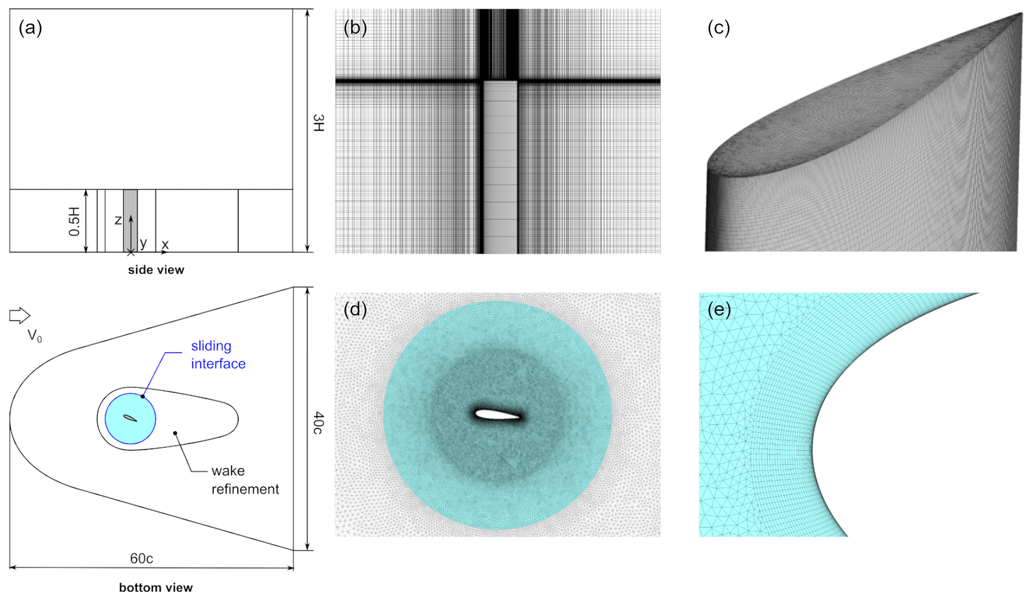
Figure 3Overview of the grid used for blade-resolved simulations: (a) computational domain, (b) side view of the mesh corresponding to the wing, (c) detail of the surface mesh at the wing tip, (d) detail of the rotating region at the wing midspan, and (e) detail of the prismatic grid used for the boundary layer discretization at the blade leading edge.
The discretization strategy is selected to ensure the optimal resolution of the vorticity distribution along the blade span as well as in the wake, i.e., the tip vortex, at a minimum computational cost, following the results of a sensitivity analysis performed by some of the authors in a previous study (Melani et al., 2022). Details of this setup are reported in Table 1.
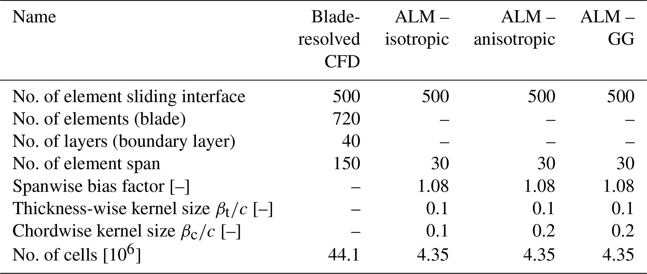
Table 1Characteristics of the grids used for the BR-CFD and ALM simulations in the present work.
A uniform Cartesian grid is used for the ALM region normal to the wingspan (blue square in Fig. 2c), as required by the ALM method, scaling the local cell size hALM on the kernel dimension under the constraint for stability reasons. The criterion adopted for the dimensioning of the smearing radius β varies with the kernel shape. For the standard isotropic function, a value of c, ensuring a correct description of the tip vortex core, is selected (Melani et al., 2022). Differently, the anisotropic and Gauss–Gumbel functions are tuned instead to minimize the error in terms of velocity field with respect to BR-CFD in a 2D environment (Mohamed et al., 2022). As this process does not consider tip effects, the setup of these two functions might not be optimal for the scope of this study. Therefore, possible conclusions about their application must be verified in future work. The ALM region is progressively expanded to the domain boundaries via an unstructured, quadrilateral mesh, always scaling the local cell size on hALM. The bottom grid is then extruded along the blade span, optimizing the grid density at the tip by distributing the elements according to an exponential bias, as shown in Fig. 2b–e (Melani et al., 2022). For further details, refer to Melani et al. (2021b).
The blade-resolved CFD simulation employs the same numerical schemes, computational domain, and meshing strategy of the ALM ones (see Sect. 2.2). However, important differences, visible in Figs. 2 and 3 and reported in Table 1, exist in the wing region due to the presence of the airfoil geometry. According to the experience of the authors in similar test cases (Balduzzi et al., 2021), the blade surface is modeled as a smooth no-slip wall, discretized with an O-type grid of 720 quadrilateral elements. To ensure a proper resolution of the boundary layer, a dimensionless wall distance (y+) lower than ∼1 and a total number of 40 layers are employed in the direction normal to the wall (see Fig. 3e). Given the Reynolds number used in the tests (see Table 3), an intermittency transport equation is added to the k–ω SST model to include the effects of turbulent transition.
The wing region is connected to the far-field domain, this time discretized with an unstructured, triangular mesh, via a sliding interface (see Fig. 3d), so it can be rotated by the imposed blade pitch angle. The final, 3D mesh is once again obtained by extruding the bottom one along the blade span. In this case, the cells are distributed not according to an exponential bias like in the ALM but assigned to the cell blocks of variable height from the midspan to tip (see Fig. 3b–e). This strategy ensures better control of the aspect ratio of the elements along the wing surface, preventing in particular the excessive stretching of those at the midspan (Balduzzi et al., 2017).
Two different families of postprocessing techniques are applied to the results of both the BR-CFD and the ALM simulations. On one hand, the most recent vortex identification methods (VIMs), described in Sect. 4.1, are adopted to outline the structure and decay of the tip vortex. On the other hand, the blade spanwise flow field is analyzed via the LineAverage technique for the sampling of the local angle of attack, whose details can be found in Sect. 4.2.
4.1 Tip vortex tracking metrics
The various modeling strategies analyzed in this work, in turn, affect the tip vortices shed from the airfoil. Hence, the effect of the applied methodology on the vortex structure is investigated through multiple metrics, namely vortex center position, core radius, and circulation. These properties are affected by viscous decay, as the vortex is convected downstream, so the analysis is performed over four vertical sampling planes with varying distance from the airfoil (1, 2, and 5 chords), starting from the aerodynamic center (see Fig. 4).
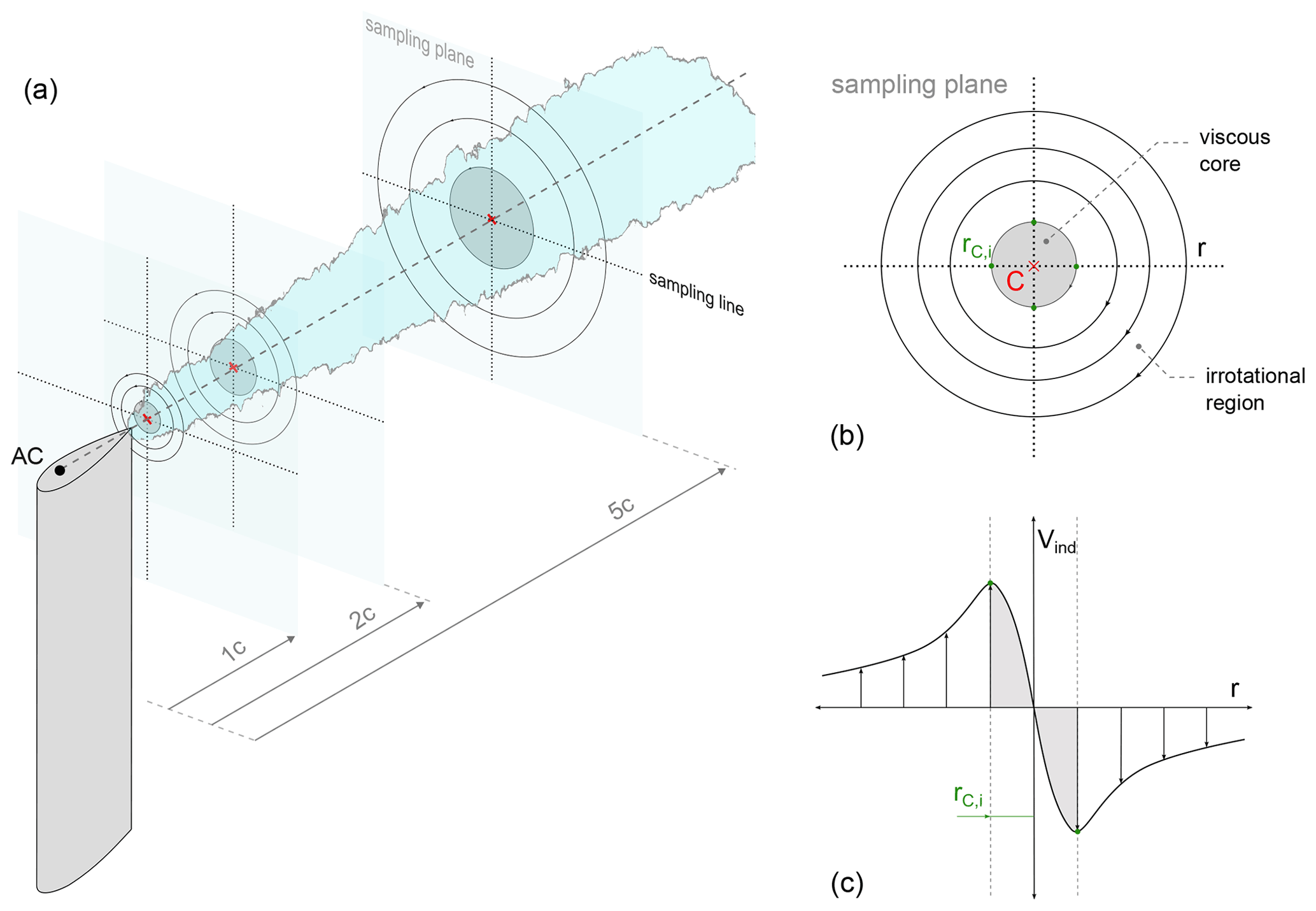
Figure 4Schematic representation of the sampling setup used in the present work: (a) the sampling planes, (b) vortex sketch and definition of core radius, and (c) velocity profile of the vortex.
As summarized in Fig. 4, the tip vortex metrics are computed following the methodology commonly used in the literature (van der Wall and Richard, 2006; Soto-Valle et al., 2022):
-
Vortex center C. The vortex center defines the axis of rotation of the vortical structure, and it is used to track the position of the tip vortex as it is convected downstream. In the present work, its position is computed from the resolved velocity field by calculating the λ2 scalar field (Jeong and Hussain, 1995) and locating the position of its minimum on the sampling plane. This methodology is selected among the available vortex identification methods as it can distinguish the contributions of viscous stresses and irrotational straining.
-
Vortex core radius rC. The core radius defines the size of the inner part of the vortex, where the fluid rotates as a rigid body. As the tip vortex is convected downstream, the vortex structure is dissipated due to viscous decay, and the size of the core increases (vortex aging). In this work, the core radius is calculated from the induced velocity field as the distance between the vortex center C and the location of maximum induced velocity Vind (Mauz et al., 2019) (see Fig. 4). Vind is calculated by subtracting the convection velocity (uc, vc) of the vortex from the velocity field as follows:
The convection velocity is assumed to be equal to the velocity in the vortex center, where the vortex-induced velocity is 0 (Yamauchi et al., 1999; van der Wall and Richard, 2006):
The core radius is calculated from horizontal and vertical slices of the induced velocity field, passing by the vortex center. In this way, the velocity profile of the vortex (see Fig. 4) is obtained along the two directions. The results are averaged to provide a more representative value. Additionally, the aspect ratio (AR) of the vortex, defined as the ratio between the average core radii in the horizontal and vertical directions, is calculated as to account for possible asymmetry of the vortical structure.
-
Vortex circulation Γ. Circulation is a measure of the vortex intensity and is used alongside the core radius to measure its aging in the wake. In this work, it was computed as the integral of the in-plane vorticity ωx. To avoid the inclusion of spurious contributions, the integration domain is centered on the vortex center and limited to a radius of 2 c from the vortex center.
4.2 Angle of attack sampling
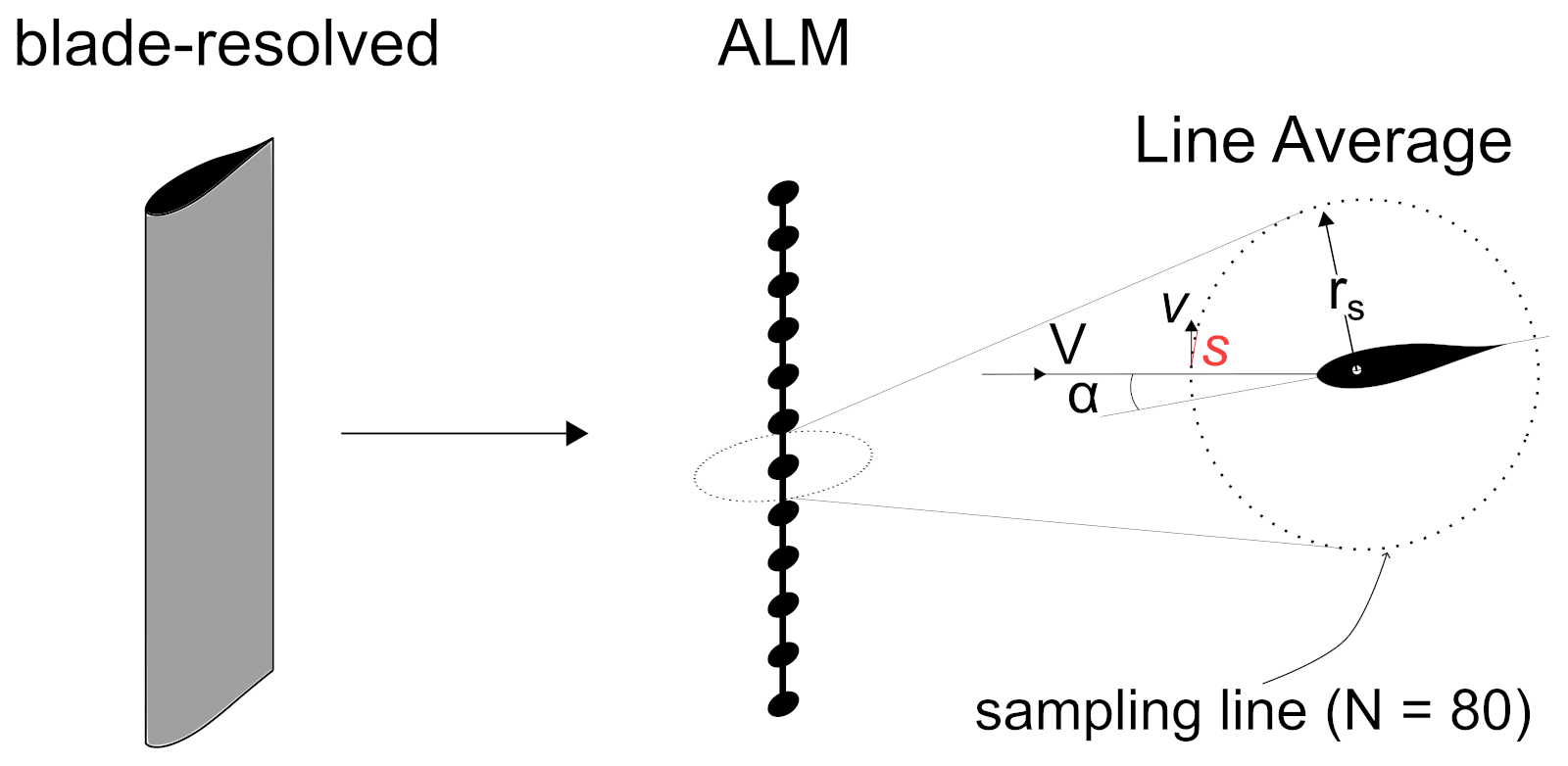
The LineAverage method was originally introduced by Jost et al. (2018) for HAWTs, in an attempt to increase the accuracy of previously available methods that capture the effects of shed and trailing vorticity on the measured angle of attack on turbine blades. To this end, the undisturbed velocity vector V is computed as the integral average of the flow velocity field along a closed line around the airfoil (see Fig. 5):
where vj is the local velocity, tangential to the sampling plane, and sj the arc length at the node j along the sampling circle. According to its creators, this sampling strategy should be able to completely remove the effect of bound circulation on the local inflow velocity, since in the averaging process the induced velocity components on any pair of opposite points on the closed path are leveled out, still accounting for the net distortion associated with shed and trailing vorticity.
The choice of this method for the present investigation is justified by the accuracy and robustness shown in (i) a previous study of some of the authors on blade-resolved simulations of vertical-axis wind turbines (Melani et al., 2020), in which it has been validated against high-fidelity numerical and experimental data, and (ii) its application to ALM simulations of both horizontal- (Bergua et al., 2023) and vertical-axis machines (Melani et al., 2021a, b).
The analysis carried out in the present work uses a sampling radius rs=1 c and N=80 evenly distributed sampling points, as recommended by Jost et al. (2018) and Rahimi et al. (2018).
In this section, the main outcomes of the investigation are presented. In Sect. 5.3, a deeper insight into the physical mechanism responsible for the load degradation observed in the reference blade-resolved simulations is provided. Although partially redundant with respect to what is found in the literature, this passage is considered fundamental by the authors to give rigor and consistency to the following analyses on the actuator line method. These are carried out in Sect. 5.4, by comparing the frozen ALM (F-ALM), combined with the different kernels outlined in Sect. 2.1, with the standard ALM (using only the isotropic function) in terms of (i) wing loads (Sect. 5.4.1), (ii) spanwise flow field (Sect. 5.4.2), and (iii) tip vortex structure (Sect. 5.4.3). This way, the error introduced by adopting a version of the ALM that is not tailored to the resolution of tip vortices can be quantified.
5.1 Test case
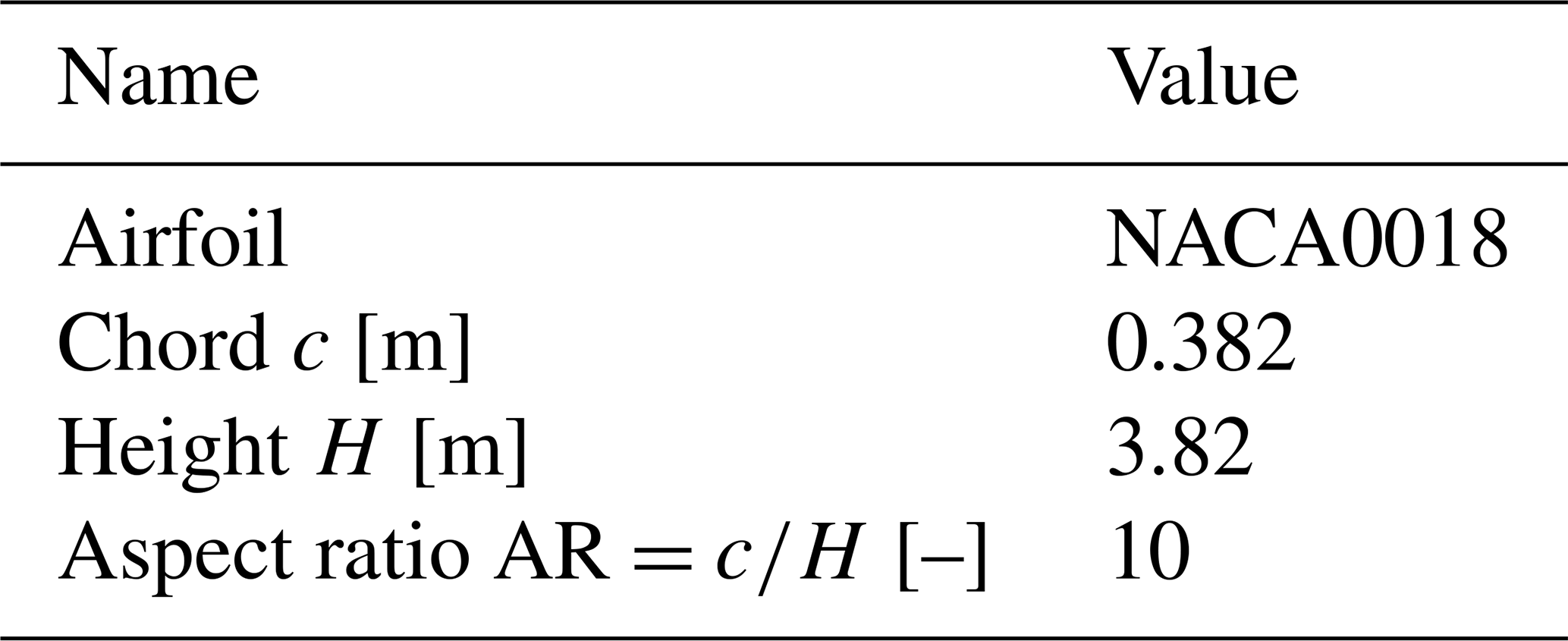
For the simulation campaign, a constant-chord NACA0018 wing is selected, whose geometrical characteristics are reported in Table 2. The choice of such a simple test case is justified by the necessity of reducing the number of governing parameters involved as much as possible, thus increasing the generality of the analysis and minimizing the possibility of biases. For instance, having a constant chord c along the span ensures that the observed load reduction towards the tip was only related to the presence of the tip vortex, without the spurious contribution of the blade tapering as in many studies on the subject (Jha et al., 2014; Churchfield et al., 2017; Martínez-Tossas and Meneveau, 2019; Meyer Forsting et al., 2019).
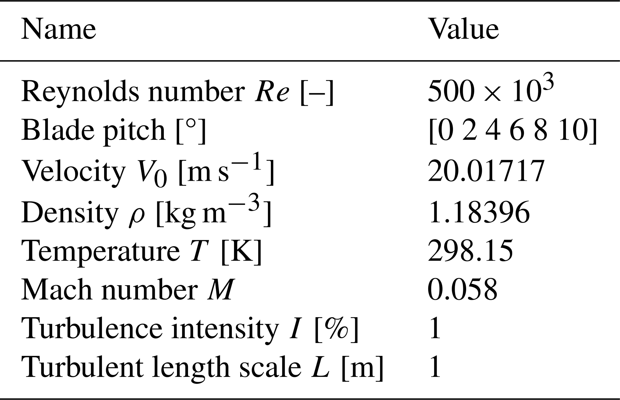
This test wing is simulated in the operating conditions reported in Table 3. The freestream, chord-based Reynolds number is selected for this airfoil to obtain a behavior of the lift curve that is as linear as possible at the considered loading conditions, i.e., low (pitch of 6°), middle (pitch of 8°), and high loads (pitch of 10°), without excessively raising the computational cost as it would happen in a high-Reynolds case. Accordingly, turbulence intensity is higher than in standard wind tunnel conditions to stabilize laminar transition in BR-CFD simulations. The inlet Mach number M is kept at a minimum to avoid compressibility effects.
5.2 Validation of BR-CFD simulations
The setup from Sect. 3 is validated, at least for the 2D case, against the experimental measurements of Timmer (2008), as shown in Fig. 6. It is observed how the matching between 2D numerical results and experiments is good until AoA = 10°, with a nearly perfect matching in terms of slope of the lift curve and drag value at the zero-lift point. Approaching the static stall point, the two datasets start diverging, as the stall predicted by BR-CFD occurs earlier than the measured one. This issue does not affect the present study, as the analysis is limited to the attached flow region, with a maximum tested angle of attack of 10° (see Table 3), thus justifying the use of 2D BR-CFD polar data for both the reconstruction of the equivalent angle of attack from BR-CFD simulations of the finite wing (see Sect. 5.3) and the standard ALM simulations (see Sect. 5.4).
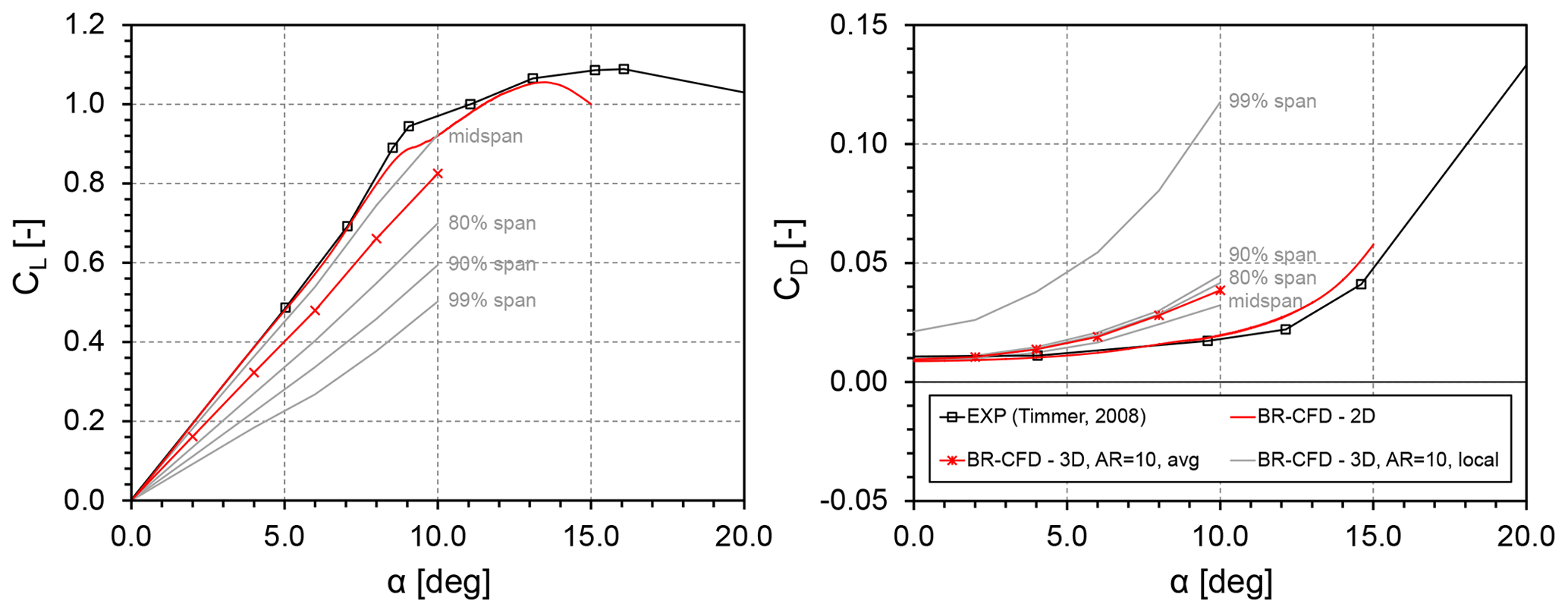
Figure 6Comparison in terms of lift (CL) and drag (CD) coefficients between the BR-CFD simulations, both 2D and 3D, and the experimental measurements from Timmer (2008), for .
On the other hand, the accuracy of 3D BR-CFD simulations cannot be verified, as no reliable data for this test case are currently available in the literature. The confidence in the adoption of these results indeed derives from (i) the experience of some of the authors in these kinds of simulations (Balduzzi et al., 2017) and (ii) the physical soundness of the results presented in Fig. 6, where the lift computed at specific sections of the wingspan (here called “local”) decreases going towards the tip, while the drag presents an abrupt increase in the last 1 % of the wing. The corresponding 3D curves, obtained from pressure integration over the wing surface, lie somewhere in between and are closer to the local ones at midspan. (iii) And, finally, confidence is also derived from the nature of the current analysis, whose aim is not to provide a benchmark for this test case but rather some insights into the physical mechanism underlying tip losses and the capability of the ALM to reproduce tip effects.
5.3 Investigation of the flow mechanism
A preliminary and fundamental step of the present investigation was the identification of the physical mechanism underlying the spanwise load degradation observed in the blade-resolved (BR-CFD) simulations taken as reference. It was indeed a priority to understand if this mechanism actually falls in the spectrum of the aerodynamic phenomena interpretable as a dynamically equivalent variation in a 2D angle of attack, as prescribed by the lifting line theory (LLT) (Prandtl and Tietjens, 1934), or if it is characterized by inherent 3D characteristics. In fact, only in the first case would the ALM have the possibility to capture the effect of tip vortices on the blade loads without the need for semi-empirical corrections, as it is based on the use of tabulated polar data. This work would then have a solid theoretical foundation. In the second case, oppositely, the only way to improve the ALM accuracy would be to rely on dedicated corrections such as the ones currently used for the simulation of wind turbines (e.g., Glauert, 1935; Shen et al., 2014).
For this purpose, a 2D angle of attack, α2D,eq, was computed for each spanwise section of the blade. As for blade-resolved simulations, it is not possible to use the LineAverage method (see Sect. 4.2) for radii lower than the airfoil chord. Since the sampling line would intersect the airfoil surface, a different strategy was adopted, following the work of Soto-Valle et al. (2020, 2021). In greater detail, α2D,eq was selected as the angle of attack that, when imposed onto a 2D calculation, would minimize the error of the predicted pressure coefficient CP (Eq. 10) distribution along the chord with respect to the one of 3D BR-CFD. It was a priority in this process to match the minimum CP value on the suction side (SS), as in the attached flow regime it is the main variable regulating lift production.
In this case, the viscid panel method used in the original approach of Soto-Valle et al. (2021) was replaced with 2D BR-CFD, using the same airfoil meshing strategy and turbulence modeling of 3D simulations (see Sect. 3). In this way, the bias in the computation of α2D,eq, related to the inherent differences between CFD and panel methods, is avoided.
Figure 7 presents the results of the workflow described above, along with the corresponding velocity field, for the low-load case (pitch of 6°). For the sake of brevity, only a few relevant blade sections are shown in the picture. The spanwise load degradation associated with the tip vortex can be reasonably approximated with a reduction in the equivalent 2D angle of attack α2D,eq until 80 % of the blade span. Consequently, the deviation between the section lift coefficient computed at α2D,eq and the 3D one is limited, as shown in Fig. 9. Therefore, this flow region is here called the 2D region. This effect is also visible from the non-dimensional velocity field, with the simultaneous rotation of the pressure side (PS) stagnation region around the airfoil leading edge and reduction in the SS suction peak.
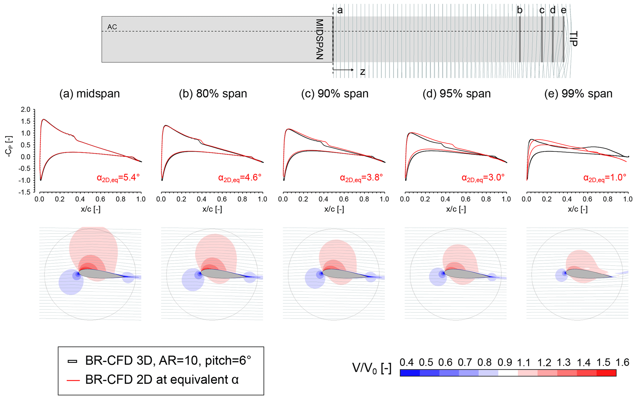
Figure 7Extraction of the pressure coefficient CP profile and non-dimensional velocity field from 3D BR-CFD from different sections along the blade span, for a pitch of 6°. The 3D pressure data are compared with those coming from the 2D BR-CFD simulations for the computation of the equivalent angle of attack α2D,eq.
The same trend is found between 80 % and 97 % of the span. Going towards the tip, however, a pressure deviation of increasing intensity arises between 3D and 2D BR-CFD in the rear of the blade () towards the trailing edge, despite the good correspondence between the two datasets in the leading edge region. This phenomenon, called the decambering effect, is well known in the literature (Sørensen et al., 2016) and derives from the radial outflow generated by the tip vortex structure. Traces of this pattern are visible in Figs. 7d–e and 8d–e (bottom) as a deviation of the freestream velocity vectors towards the SS wall. Since in this part of the blade the flow progressively becomes 3D and the deviation between 2D and 3D lift coefficients is increasing (see Fig. 9), the corresponding blade section is called the transition region.
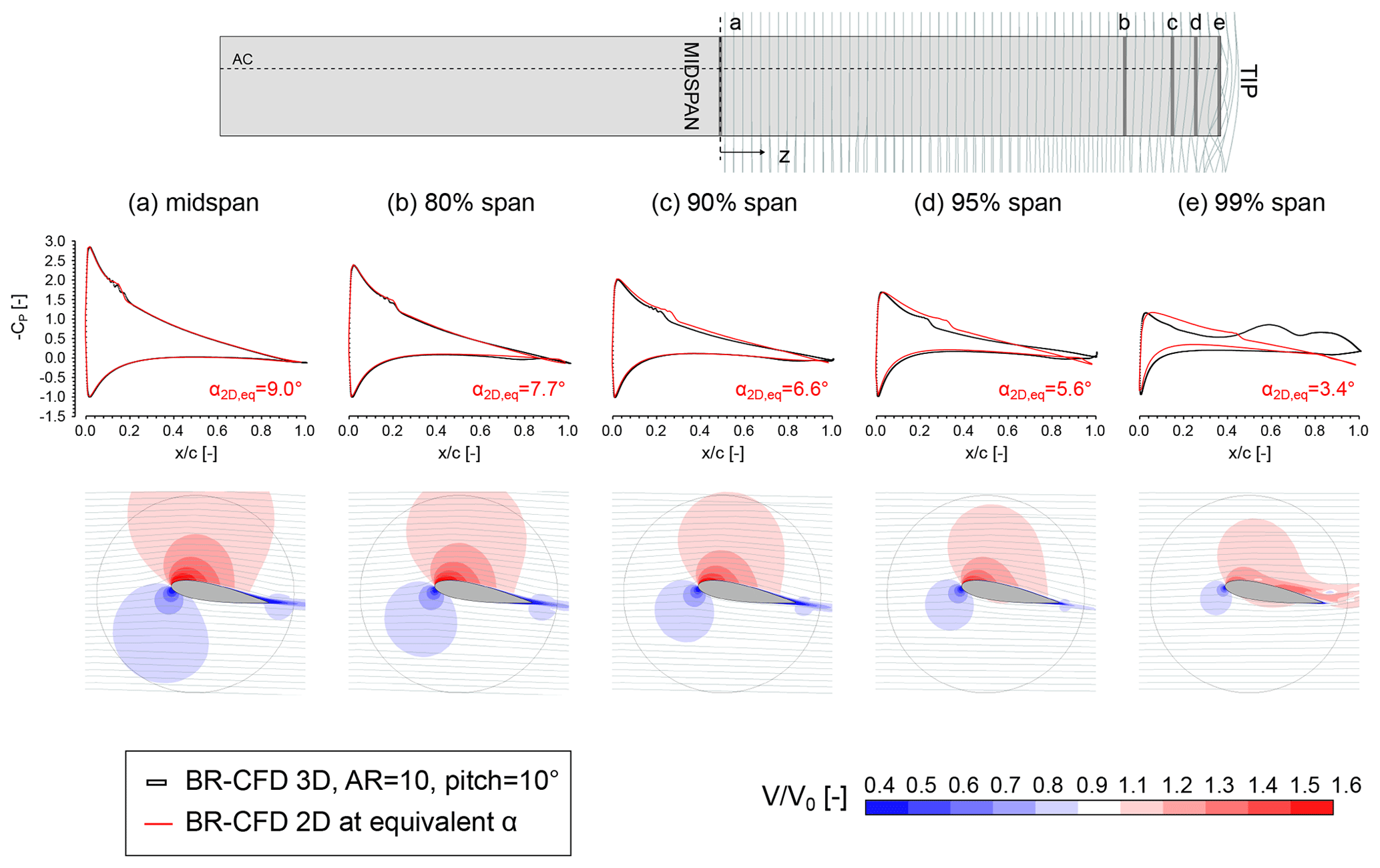
Figure 8Extraction of the pressure coefficient CP profile and non-dimensional velocity field from 3D BR-CFD from different sections along the blade span, for a pitch of 10°. The 3D pressure data are compared with those coming from the 2D BR-CFD simulations for the computation of the equivalent angle of attack α2D,eq.
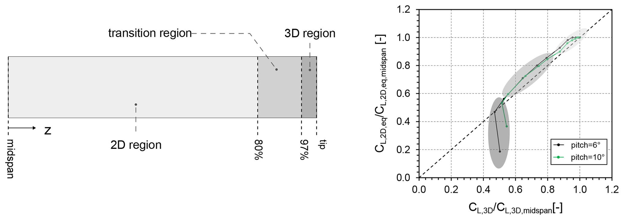
Figure 9Normalized plot of the lift coefficient computed from α2D,eq vs. the one directly extracted from the 3D BR-CFD simulations. The amount of deviation from the ideal situation in which the two are the same is used to identify the different flow regimes developing along the blade span.
Differently, in the region between 97 % of the span and the tip, the flow becomes fully 3D (3D region) so that 2D theory and the concept of angle of attack itself lose validity (Branlard, 2017). Indeed, it is not possible anymore to approximate the blade loads using polar data, as testified in Fig. 9 (right). The extension of this region and the intensity of the corresponding loads are small enough though for the hypothesis of an α2D,eq to still be adopted, confirming the prescriptions of the lifting line theory.
As the same considerations can be made for the high-load scenario (pitch of 10°) presented in Fig. 8 without losing coherence, it is possible to conclude, at least for this specific case, that the effect of tip vortices on a resolved flow field can be reasonably approximated as an angle of attack reduction. A corollary of this conclusion is that the ALM can, in theory, reproduce this effect without resorting to additional corrections. Whether this is actually feasible or not is investigated in Sect. 5.4. A feature of the blade spanwise flow that is apparent from Figs. 7 and 8 and should not be ignored is that the reduction in α2D,eq does not happen in the freestream, which remains basically undisturbed, but at the blade chord scale. This is key when deciding on the velocity sampling strategy, as is later explained in Sect. 6.
5.4 ALM
As discussed, Sect. 5.3 demonstrates that, at least for this test wing, the main mechanism responsible for the spanwise load degradation observed in the BR-CFD results is a progressive reduction in the local equivalent angle of attack α2D,eq. This confirmed the assumptions of lifting line theory. Starting from there, the question naturally arose whether the ALM can reproduce the flow field observed in the BR-CFD simulations, both along the blade span and in the wake, and how this information can be properly extracted from the resolved velocity field for the computation of blade loads. To make the analysis as general as possible, three different kernel shapes from the literature are considered: the standard isotropic Gaussian and two new formulations, namely anisotropic Gaussian and Gauss–Gumbel (see Sect. 2.1). The standard LineAverage sampling line at rs=1 c is also reported for clarity.
5.4.1 Wing loads
The analysis starts from the benchmarking of the LineAverage method (see Sect. 4.2) in its standard setup (rs=1 c), i.e., the one that is commonly found in the literature and provides good results for 2D flows. The angle of attack sampled from the flow field with this method will from now on simply be referred to as α and must be distinguished from the equivalent 2D angle of attack α2D,eq that was reconstructed from the BR-CFD simulations by comparing the airfoil pressure data.
Figure 10 reports the α spanwise profile for BR-CFD, frozen ALM (from here on abbreviated as F-ALM), and standard ALM, for the three load conditions considered in this work, i.e., low (pitch of 6°), middle (pitch of 8°), and high loads (pitch of 10°). For the sake of clarity, only the curves of the isotropic case are reported, as changing the kernel shape provided no relevant difference. The three datasets are in good agreement with each other, although both standard ALM and F-ALM tend to filter out some of the flow oscillations observed in the BR-CFD simulations, and they predict an angle of attack that increases going towards the tip.
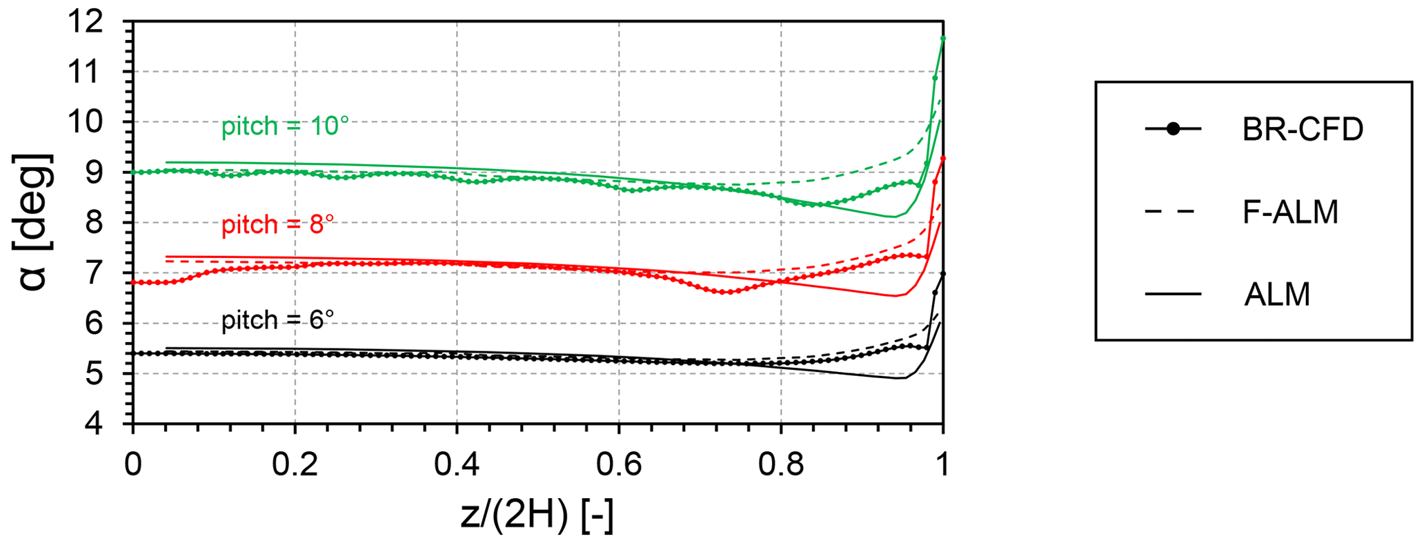
Figure 10Comparison between BR-CFD, frozen ALM (F-ALM), and standard ALM for the three operating conditions under consideration in terms of angle of attack sampled with the standard LineAverage setup (rs=1 c). As the three kernel shapes yield the same results, only the data for the isotropic function are reported.
As this trend does not follow the one observed in Sect. 5.3 and, more generally, the common understanding of the phenomenon, relevant discrepancies arise when the sampled angle of attack is cross-compared with the corresponding blade forces (see Fig. 11). The crosswise force coefficient Cy predicted by the standard ALM, which scales linearly with α, starts deviating from the 3D BR-CFD one – computed by integrating the blade pressure distribution – already at 60 % of the span, keeping a constant profile before increasing at 90 % of the span. In contrast, the BR-CFD simulations show a decreasing trend up to the tip of the blade. Looking at the streamwise force coefficient Cx, the difference seems smaller for most of the blade span but only because the drag coefficient CD is approximately constant in the attached flow region (see Fig. 6).
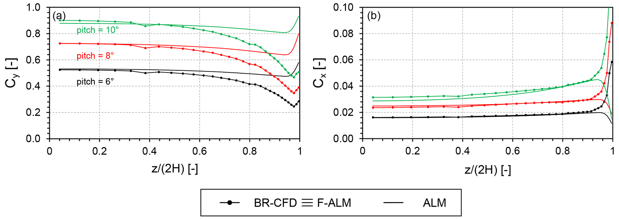
Figure 11Comparison between BR-CFD, frozen ALM (F-ALM), and standard ALM for the three operating conditions under consideration in terms of (a) force coefficient along the crosswise direction and (b) force coefficient along the streamwise direction. As the three kernel shapes yield the same results, only the data for the isotropic function are reported.
At the tip, where the flow is fully 3D (see Sect. 5.3), the 3D BR-CFD and ALM profiles deviate abruptly due to the induced drag associated with the shedding of the tip vortex. However, this phenomenon lies outside of the range of validity of 2D airfoil theory, upon which the ALM and all methods based on polar data are built, and therefore outside of the scope of the present study.
5.4.2 Spanwise flow
To gain a deeper insight into the apparently unphysical behavior observed in Sect. 5.4.1 and, more generally, into how the flow field along the blade develops for the different simulation methods, Figs. 12 and 13 report the comparison in terms of non-dimensional velocity between BR-CFD, F-ALM, and ALM, along different spanwise locations, for a pitch of 6° and a pitch of 10°, respectively. The standard LineAverage sampling line at rs=1 c is also reported for clarity.
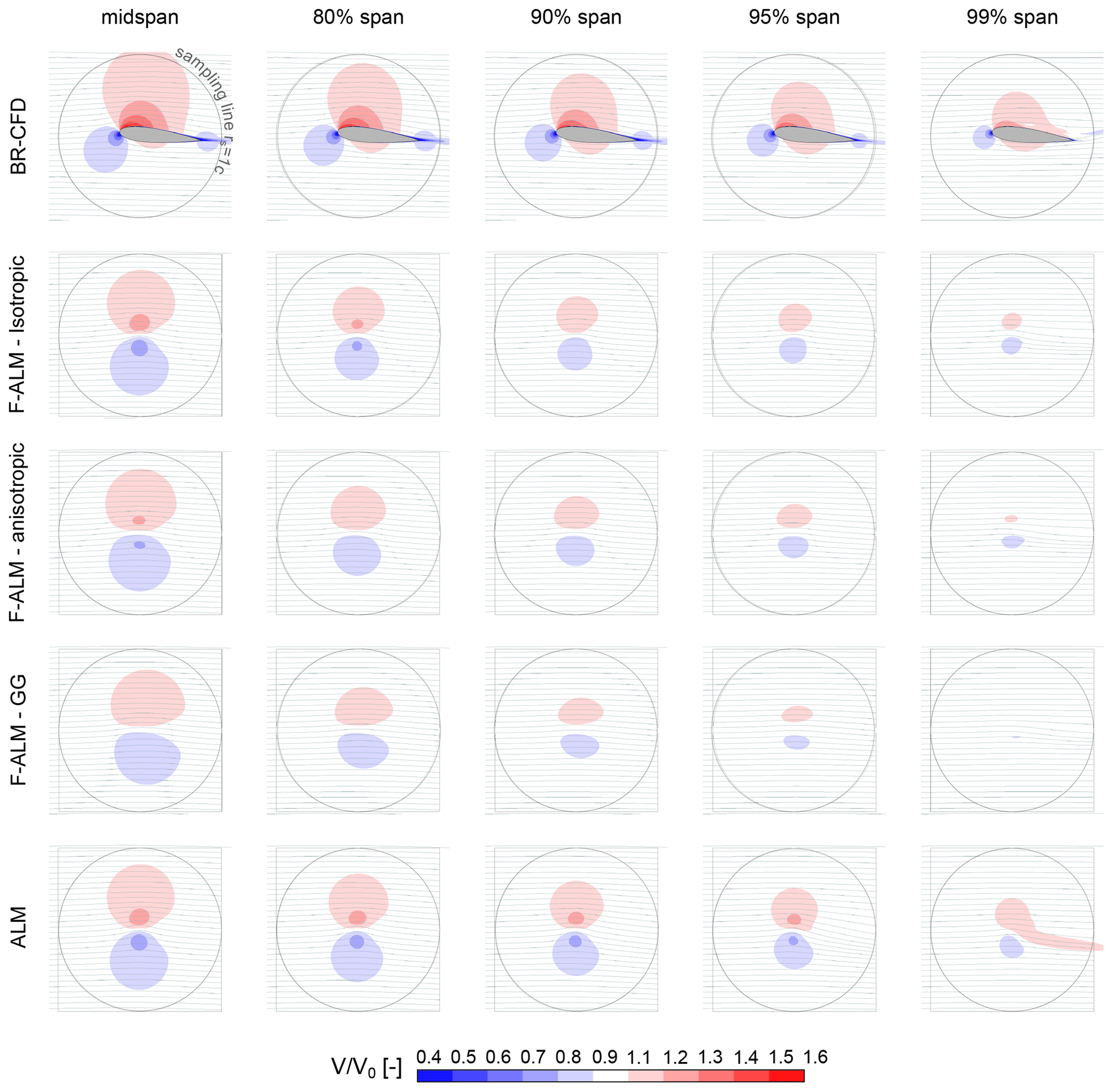
Figure 12Comparison in terms of the non-dimensional velocity magnitude between BR-CFD, frozen ALM (F-ALM), and standard ALM (ALM) at different spanwise sections, for a pitch of 6°.
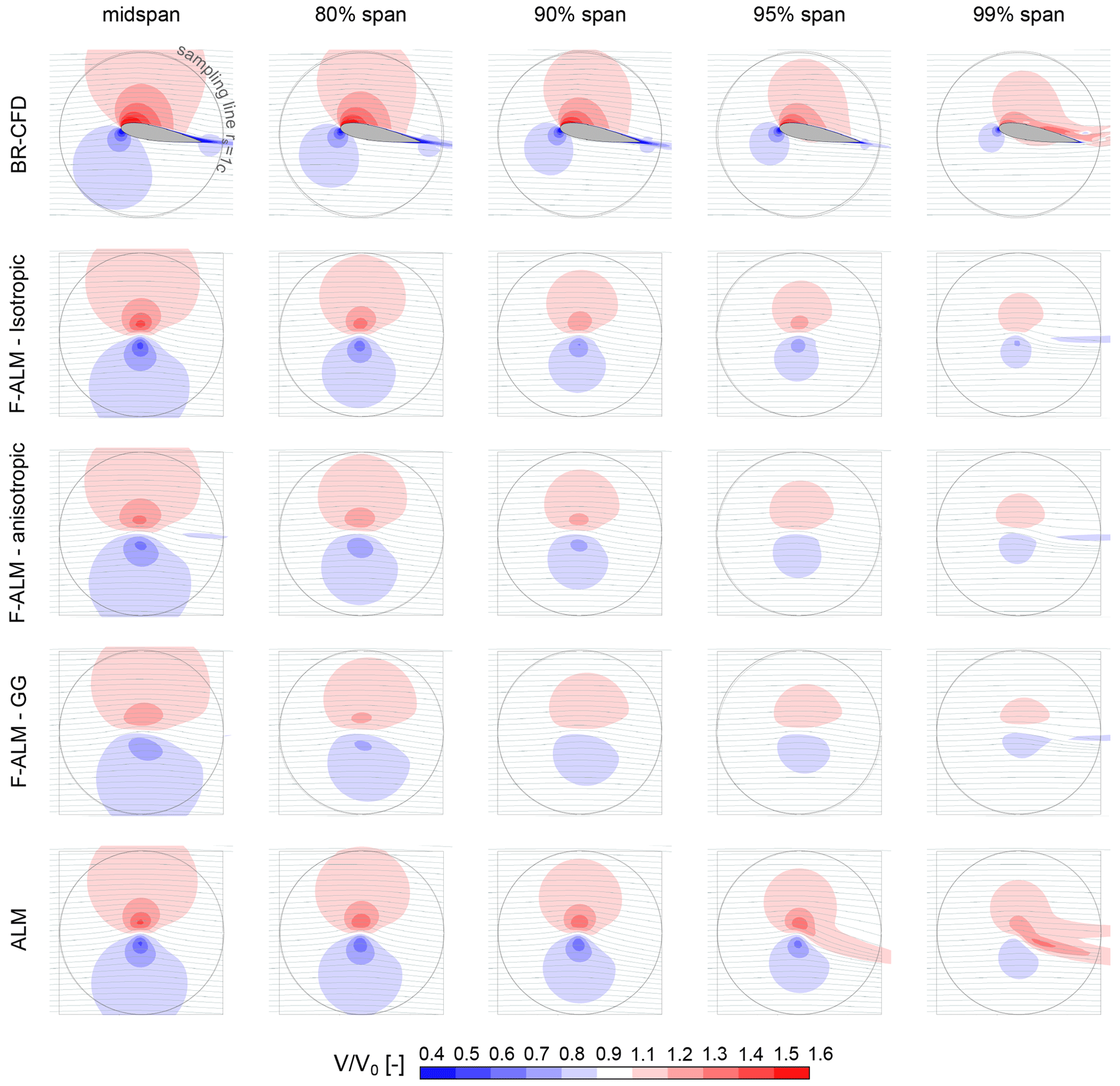
Figure 13Comparison in terms of the non-dimensional velocity magnitude between the BR-CFD, frozen ALM (F-ALM), and standard ALM (ALM) different spanwise sections, for a pitch of 10°.
It is evident how all ALM variants produce a distortion of the velocity field along the span that is similar, at least qualitatively and with all the well-known limitations of the ALM method, to that of BR-CFD. Even the SS high-velocity bubble's progressive elongation, related to the presence of the tip vortex, is captured. The only relevant deviation is visible at 99 % of the span, where the flow becomes fully 3D, thus invalidating the assumption of 2D sectional flow that underlies all polar-based methods like the ALM (see Sect. 5.3). At the wing's midspan, the magnitude of this velocity distortion is correctly predicted by both F-ALM and ALM, regardless of the selected kernel shape. Moving towards the sections close to the wing tip (e.g., 90 % and 95 % of the span), however, the two approaches progressively diverge from one another. The F-ALM, despite having the same force distribution of BR-CFD (see Fig. 11), systematically underestimates the corresponding velocity distortion. This issue is well known in the scientific community (Jha et al., 2014; Dağ and Sørensen, 2020; Martínez-Tossas and Meneveau, 2019), where it has been justified by the loss of circulation related to the spreading of aerodynamic forces into the computational grid. The presented results further confirm this theory.
Notably, the use of non-conventional kernel shapes such as an anisotropic shape and Gauss–Gumbel exacerbates the situation by spreading forces over a wider area compared to their isotropic counterpart. The standard ALM instead predicts a spanwise evolution of the velocity field much closer to that observed in BR-CFD simulations. In this case, the discussed loss of circulation induced by the regularization kernel is compensated for by the higher lift force, i.e., higher circulation magnitude, given by the ALM in the last 40 % of the blade span (see Fig. 11).
To better quantify the differences in the spanwise circulation distribution predicted by each simulation method and link them to the corresponding sampled angle of attack profile (see Fig. 10), Fig. 14 reports the comparison between BR-CFD, F-ALM, and ALM in terms of non-dimensional crosswise velocity : this quantity is equivalent to the non-dimensional downwash velocity induced by the tip vortex on the wing plane. Only the high-load case (pitch of 10°) is considered here for the sake of brevity.
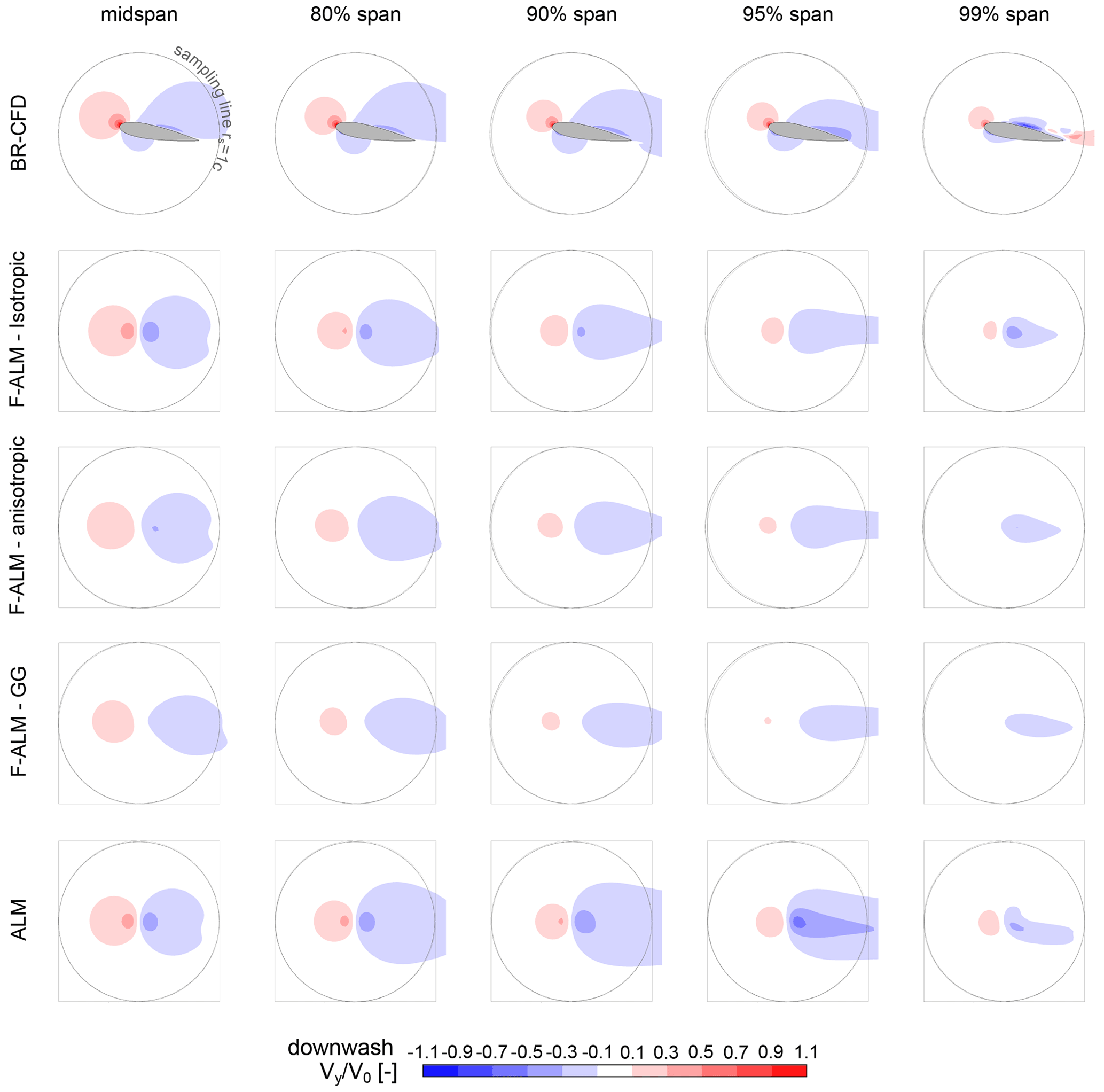
Figure 14Comparison in terms of the non-dimensional downwash velocity between the BR-CFD, frozen ALM (F-ALM), and standard ALM (ALM) at different spanwise sections, for a pitch of 10°.
Focusing at first on the midspan plane, it is observed that the induced velocity field is dominated by the airfoil bound circulation, which is connected to the generated lift. In BR-CFD, its effect, although distributed along the airfoil chord, can be reduced to upwash () and downwash () bubbles positioned at the leading and trailing edges, respectively.
This pattern is well approximated in the far field by F-ALM and ALM, using the distribution typical of a Lamb–Oseen vortex – anti-symmetric with respect to the flow normal direction – as prescribed by classic ALM theory (Shives and Crawford, 2013). It must be noted that a small difference in size between the upwash and downwash bubbles is still present due to the influence of the tip vortex. In this situation, the standard LineAverage setup (rs=1 c) works as intended, giving an α estimation that is coherent between BR-CFD, F-ALM, and ALM (see Fig. 10) and close to the reference α2D,eq from Sect. 5.3. The sampling line lies, in fact, in a relatively undisturbed flow region (LineAverage was indeed first applied in ALM for wind turbine simulation (Melani et al., 2021a) to capture the local deceleration of the flow without including the contribution of bound vorticity).
Moving towards the tip, due to the simultaneous decrease in airfoil bound circulation and increase in the tip vortex strength, the effect of the vortex-like pattern previously observed at the midspan is progressively concentrated around the airfoil aerodynamic center (AC). In the process, the balance in size between the upwash and downwash bubbles is progressively broken, as the tip vortex slows down the size reduction in the downwash bubble in the rear part of the airfoil and stretches it in the wake direction.
This effect is visible from the BR-CFD, F-ALM, and ALM simulations but with relevant differences in the magnitude of the phenomenon. As a consequence of the tendency to overestimate the reduction in local circulation along the span (already observed in Figs. 12 and 13), all F-ALM simulations exaggerate the size difference between the front positive and the rear negative induction regions with respect to BR-CFD. Once again, the use of non-standard kernel shapes accentuates this trend, especially at the sections at 95 % and 99 % of the span. When using the standard ALM, on the other hand, the balance between bound circulation and the trailing vorticity related to the tip vortex is partially restored, better capturing the distribution observed in BR-CFD than the F-ALM approach. A relevant improvement in the prediction of the lateral extension of the downwash region in the rear part of the wing is also achieved. This time, the standard LineAverage setup (rs=1 c) is not able to follow the progressive concentration of the induction pattern around the airfoil AC (see Fig. 14), missing most of the downwash induced by the shed vortex and thus yielding the unphysical values for the angle of attack observed in Fig. 10.
5.4.3 Tip vortex structure
Figure 15 shows the comparison in terms of non-dimensional downwash velocity between blade-resolved CFD (BR-CFD), frozen ALM (F-ALM), and standard ALM (ALM) for three different load/pitch conditions. The downwash velocity is sampled in the near wake, along a line one chord away from the blade AC.
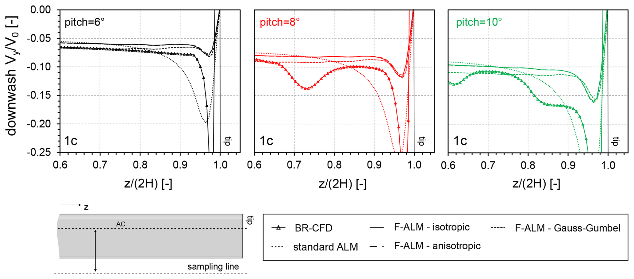
Figure 15Comparison in terms of the spanwise non-dimensional downwash velocity between BR-CFD; frozen ALM (F-ALM) for isotropic, anisotropic, and Gauss–Gumbel kernel shapes; and standard ALM at the three operating conditions under consideration.
It is apparent that the F-ALM gives a fair estimation of the downwash immediately downstream of the wing trailing edge (x=1 c) up to 80 % of the span, then rapidly loses accuracy in the last 20 %. In fact, the magnitude of the velocity induced by vortices in the tip region is heavily underestimated, consistent with the fact observed in Sect. 5.4.2 that F-ALM tends to overspread the computed forces over a wider area compared to high-fidelity simulations. The effect of the kernel shape is not as marked as on the spanwise velocity field (see Figs. 12–14), although small discrepancies between different functions are still present, especially with the Gauss–Gumbel kernel. On the other hand, when the standard ALM is used, the corresponding improvement in the description of the spanwise flow field positively reflects on the wing wake structure: the predicted downwash peak is closer in magnitude to the BR-CFD one for all loading conditions, although it extends over a spanwise region (), i.e., wider than the one observed in F-ALM.
Shifting the focus on the tip vortex structure in the near and far wake reported in Fig. 16, the differences between the F-ALM and ALM approaches are reduced, as the flow behavior is dominated by the integral balance between the bound vorticity along the blade and the one shed into the wake. In fact, the circulation Γ of the tip vortex is well predicted, proving that the ALM is conservative, although a small deviation is observed at the higher loads, e.g., a pitch of 10°. Regarding the shape of the tip vortex, it can be inferred from Fig. 16 that the F-ALM and ALM approaches, when the kernel width is properly tuned (see Sect. 2.1), provide a satisfying estimation of the BR-CFD vortex characteristics, i.e., core radius rC and aspect ratio (AR), especially in the near wake (). However, the standard ALM tends to slightly underestimate the vortex core AR. In the far wake, both F-ALM and ALM overestimate the vortex aging speed with respect to the BR-CFD, leading to the rC deviations up to +100 % at in the case of F-ALM. The results are improved when standard ALM is used, consistent with its better description of the spanwise flow evolution (see Sect. 5.4.2). In the authors' view, this accelerated vortex aging observed in the ALM simulation might be related to the absence of the turbulence generation normally occurring in the presence of a physical blade tip. A minor role might also be played by the inevitable difference in grid resolution with BR-CFD.
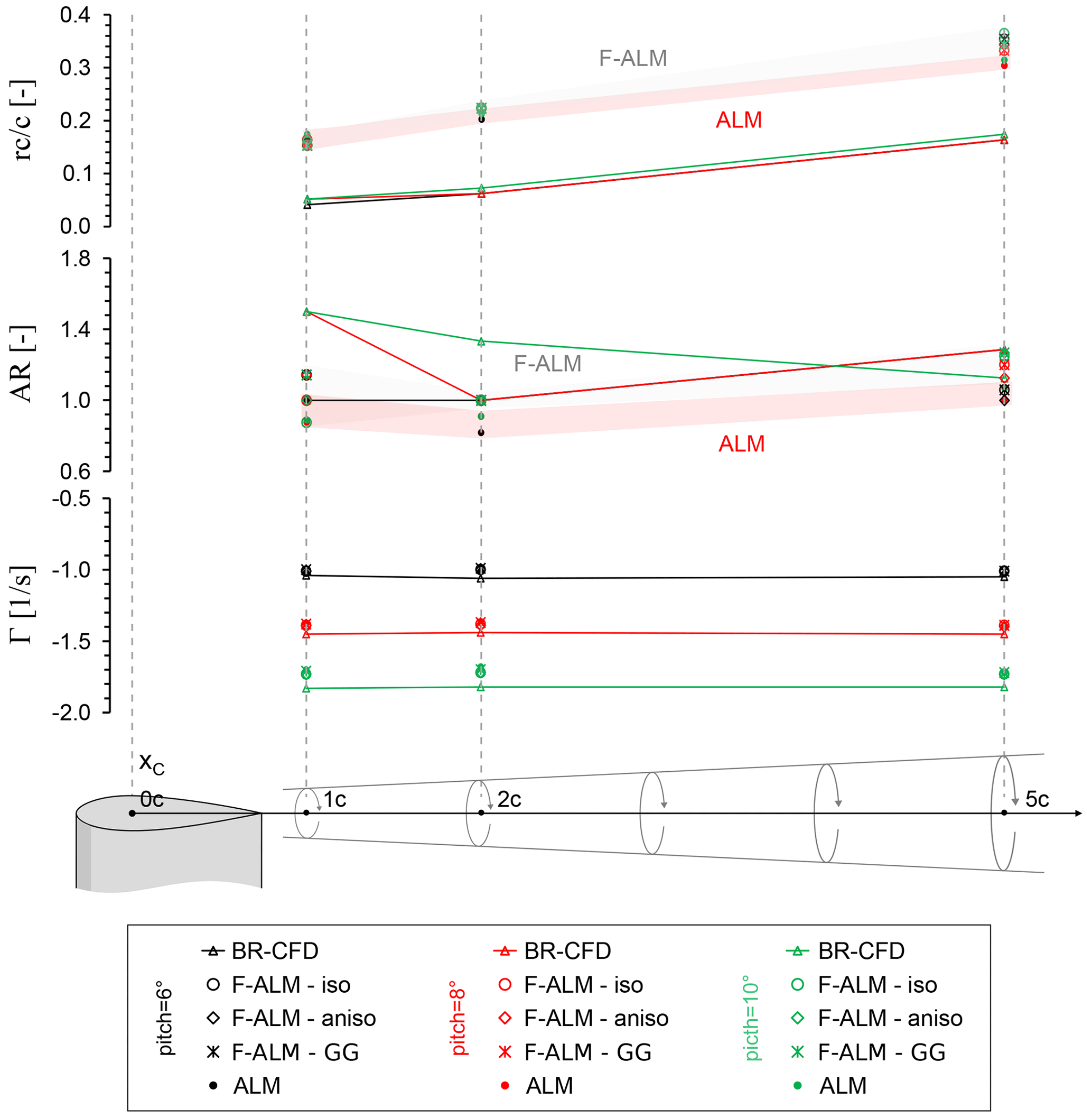
Figure 16Comparison in terms of tip vortex core radius, aspect ratio, and intensity up to five chords downstream of the airfoil between BR-CFD, frozen ALM (F-ALM) with three different kernel shapes (isotropic, anisotropic, Gauss–Gumbel), and standard ALM for a pitch of 6, 8, and 10°.
The analysis carried out in Sect. 5.4.2 and 5.4.3 established that the actuator line method can, with its own limitations, reproduce the spanwise flow distortion induced by the tip vortex and observed in BR-CFD. The LineAverage with its standard settings (rs=1 c) gives a correct estimation of the local angle of attack at the midspan, where this spanwise distortion is minimum but starts losing accuracy going towards the tip, as it misses the progressive concentration of the tip vortex trace around the airfoil AC. Based on these considerations, a natural solution to this issue would be to use the standard sampling distance of rs=1 c in the midspan part of the blade, then progressively reducing it towards the tip. This strategy was also suggested in the original paper about the LineAverage method (Jost et al., 2018) but never further developed.
In an attempt to explore the concept, Fig. 17 reports the spanwise α profiles sampled from both the F-ALM and the ALM simulations at a progressively smaller sampling radius rs. The extreme case, corresponding to rs=0, is represented by the punctual sampling along the aerodynamic center (AC) line: this is included in the comparison to establish a lower limit on the achievable probing distance and provide a useful comparison with what is currently the most common sampling approach used in ALM codes (Martinez et al., 2012; Sørensen and Shen, 2002; Shamsoddin and Porté-Agel, 2014; Bachant et al., 2018). The effectiveness of reducing the sampling radius is quantified by using the equivalent 2D angle of attack α2D,eq spanwise profiles from BR-CFD as a benchmark. The analysis is carried out in low- (pitch of 6°) and high-load (pitch of 10°) conditions. At the standard setup of rs=1 c, all ALM approaches yield the same profiles as Fig. 10, reasonably approximating the BR-CFD equivalent angle of attack α2D,eq up to ca. 60 % of the span, where the airfoil aerodynamics are still dominated by the undisturbed inflow conditions, and then largely overestimating it in the rest of the span (), where the local deformation induced by the tip vortex cannot be neglected. Progressively reducing the sampling radius, the behavior of the sampled α becomes strongly dependent on the adopted ALM approach and so, indirectly, on the spanwise force insertion strategy. Considering at first the F-ALM isotropic setup, it is observed how the α spanwise profile does not deviate significantly from the one sampled at rs=1 c until a critical sampling radius, in this case c, is used. After this point, in fact, the sampled α is shifted towards lower values of angle of attack and presents a decreasing trend with , as would be expected based on physical reasoning. Nonetheless, in the last 20 % of the wing (), this trend does not follow the reference α2D,eq from BR-CFD but maintains an approximately constant value up to and then drops abruptly. Consequently, the reference α2D,eq curve falls out of the angle of attack range covered by the family of curves sampled with the LineAverage for . This incompatibility is probably related to the tendency of the F-ALM approach to overestimate the spanwise reduction in circulation towards the tip with respect to high-fidelity simulations (see Sect. 5.4.2). The initial evidence supporting this hypothesis is that the region of incompatibility between α and α2D,eq becomes bigger when switching to non-standard kernels, where the loss of circulation due to the spreading of wing forces is even more accentuated (see Figs. 12 and 13). In the extreme case of the Gauss–Gumbel kernel, for instance, this region covers the last 40 % of the span ().
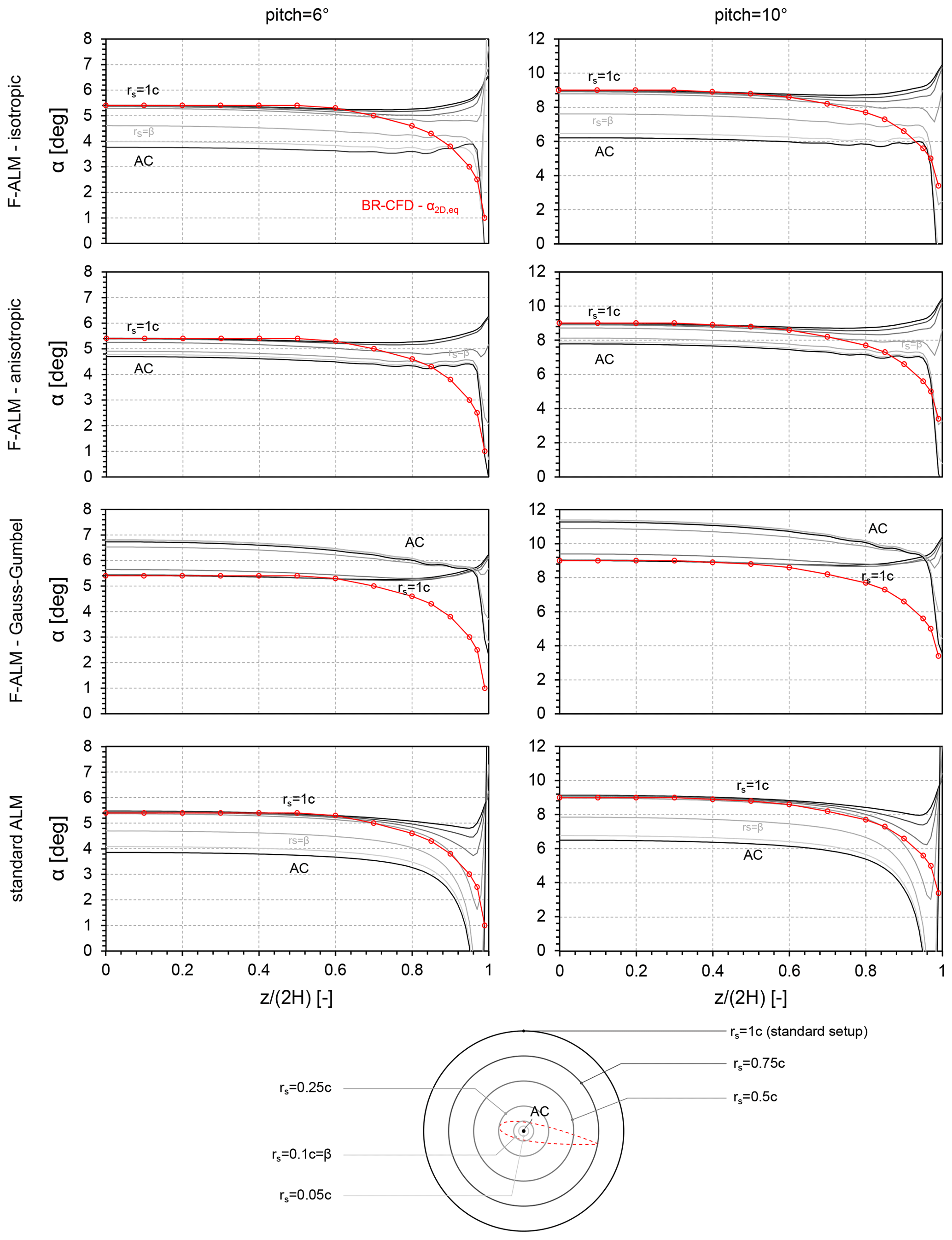
Figure 17Comparison in terms of AoA spanwise distribution between BR-CFD (calculated as a dynamically equivalent AoA), frozen ALM (F-ALM), and standard ALM (sampled via the LineAverage method at different sampling distances). The data under the name AC refer to the sampling at the aerodynamic center of the airfoil, corresponding to the force insertion point.
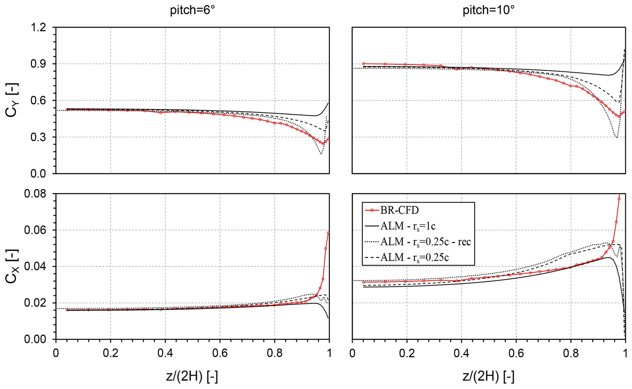
Figure 18Comparison in terms of force coefficient along the crosswise direction (CY) and force coefficient along the streamwise direction (CX) between BR-CFD and ALM with a standard (rs=1 c) and an optimal (rs=0.25 c) sampling radius. For the series denominated rec, wing loads do not come from direct simulation but are reconstructed a posteriori from the postprocessed angle of attack.
More evidence is given by the results obtained with the standard ALM (see Fig. 17). As the corresponding circulation spanwise distribution is notably closer to the BR-CFD one (see Figs. 12–14), the reference α2D,eq curve is now fully contained in the set of α curves sampled with the LineAverage at decreasing rs, removing the incompatibility observed in the F-ALM results (see Fig. 17). Therefore, the angle of attack information required by the ALM for a correct spanwise load computation can be fully extracted from the flow field. It is interesting to note that the sampling radius rs=0.1 c, which corresponds to the kernel size β=0.1 c used for the simulations, once again represents a critical threshold, in this case the minimum sampling radius required to have the complete description of the angle of attack variation along the span.
To conclude the present investigation, the newly found possibility of increasing the ALM capability to predict tip effects by tuning the α sampling algorithm is put to the test. Figure 18 reports the comparison in terms of wing loads between BR-CFD and ALM in its standard (rs=1 c) and optimal (rs=0.25 c) setup. The optimal value for the sampling radius is selected from Fig. 17 as the one providing the best match with the α2D,eq spanwise profile from BR-CFD. For completeness, the load data reconstructed a posteriori from the angle of attack data at rs=0.25 c from Fig. 17 are also shown (ALM − rs=0.25 c − rec): in this case, the inserted force field is not coupled to the sampled α but corresponds to the one of the standard ALM simulation (rs=1 c). Reducing the sampling radius to 0.25 c already provides a notable improvement in the ALM description of spanwise loads, especially CY, despite not considering the decambering effect (see Sect. 5.4.1). The abrupt increase in CX in the last 5 % of the span is related instead to inherently 3D effects and is thus out of the ALM validity range (see Sect. 5.4.1). It is worth noting that, as for the F-ALM, a better prediction of the BR-CFD spanwise load degradation corresponds to an excessive loss of circulation intensity in the tip region. This justifies the deviation visible in Fig. 18 with respect to the reconstructed load data (ALM − rs=0.25 c − rec). Different solutions to this issue are available in the literature, e.g., reducing the kernel size going towards the wing tip (Jha et al., 2014; Jha and Schmitz, 2018). These are, however, out of the scope of the present investigation and will be addressed in future work.
In this study, a comprehensive investigation on the ALM's capability to simulate tip effects has been performed. To this end, a NACA0018 finite wing was the case study for three different simulation techniques: high-fidelity, blade-resolved CFD simulations (to be used as a benchmark), standard ALM without any correction, and ALM with the spanwise force distribution extracted from blade-resolved data (frozen ALM). The analysis has been repeated for three different kernel shapes: isotropic Gaussian, anisotropic Gaussian, and Gauss–Gumbel, respectively. For the postprocessing and comparison of the data, advanced vortex identification methods for outlining the structure and decay of the tip vortex have been combined with the LineAverage technique for the sampling of the local angle of attack along the blade span.
Upon examination of the results, the following conclusions can be drawn:
-
Until the flow becomes fully 3D – in this case, until the last 5 % of the span – the spanwise load degradation observed in BR-CFD can be interpreted as a dynamically equivalent reduction in the local angle of attack. This phenomenon is confined at the blade chord scale.
-
The scale of interaction reduces when moving from a region dominated by bound circulation, such as the blade midspan, to one dominated by trailing vorticity, such as the tip. Therefore, when modeling tip effects in the ALM framework, it is key that the characteristic lengths of both force smearing and angle of attack sampling from the flow field decrease approaching the blade extremity. Numerical details of this procedure are out of the scope of the present paper and will be detailed in future work.
-
The ALM produces a more diffused vortex than BR-CFD. Correspondingly, the vortex intensity and downwash in the wake are underestimated. This deviation increases with the blade loading, i.e., pitch angle. The vortex aging on the other hand is overestimated, especially in the far wake (five chords away from the wing tip). It is not clear from the study whether this gap can be filled by improving the ALM formulation or if it is related to the intrinsic differences between ALM and BR-CFD.
-
The use of alternative kernel shapes (sometimes proposed as a countermeasure in the literature), such as anisotropic Gaussian or Gauss–Gumbel, does not introduce relevant differences in the predicted loads and tip vortex structure but lowers the capability of the ALM to extract the proper angle of attack from the flow field. Therefore, their use is not recommended.
The ALM software used in the present work is currently not available due to confidentiality issues. Scripts used for data sampling and postprocessing are available upon request.
Data postprocessed from BR-CFD, frozen ALM, and ALM simulations are available at https://doi.org/10.5281/zenodo.10809726 (Melani et al., 2024). Raw simulation data, e.g., flow fields, are available upon request due to the large file size.
PFM conceptualized the work, carried out ALM and CFD analyses, and was responsible for the first draft preparation. OSM and SC helped with the ALM analyses and vortex identification methods, respectively. FB and AB helped with orientating the research, critically discussing the analysis, and reviewing the paper. AB coordinated the research team.
At least one of the (co-)authors is a member of the editorial board of Wind Energy Science. The peer-review process was guided by an independent editor, and the authors also have no other competing interests to declare.
Publisher's note: Copernicus Publications remains neutral with regard to jurisdictional claims made in the text, published maps, institutional affiliations, or any other geographical representation in this paper. While Copernicus Publications makes every effort to include appropriate place names, the final responsibility lies with the authors.
This study is the expanded version of a preliminary study presented at the WESC 2023 conference by the European Academy of Wind Energy (EAWE). The authors would like to acknowledge Giovanni Ferrara from Università degli Studi di Firenze for supporting this activity and for the useful technical discussions.
This work did not receive external financial support. However, it has made use of a 20 % fee reduction thanks to the contribution of the European Academy of Wind Energy, being the follow-up of an oral presentation at WESC 2023.
This paper was edited by Roland Schmehl and reviewed by Luca Greco and Thomas Potentier.
Bachant, P., Goude, A., and Wosnik, M.: Actuator line modeling of vertical-axis turbines, arXiv [preprint], arXiv:1605.01449 [physics], https://doi.org/10.48550/arXiv.1605.01449, 2018.
Balduzzi, F., Drofelnik, J., Bianchini, A., Ferrara, G., Ferrari, L., and Campobasso, M. S.: Darrieus wind turbine blade unsteady aerodynamics: a three-dimensional Navier-Stokes CFD assessment, Energy, 128, 550–563, https://doi.org/10.1016/j.energy.2017.04.017, 2017.
Balduzzi, F., Marten, D., Bianchini, A., Drofelnik, J., Ferrari, L., Campobasso, M. S., Pechlivanoglou, G., Nayeri, C. N., Ferrara, G., and Paschereit, C. O.: Three-dimensional aerodynamic analysis of a darrieus wind turbine blade using computational fluid dynamics and lifting line theory, J. Eng. Gas Turb. Power, 140, 022602, https://doi.org/10.1115/1.4037750, 2018.
Balduzzi, F., Holst, D., Melani, P. F., Wegner, F., Nayeri, C. N., Ferrara, G., Paschereit, C. O., and Bianchini, A.: Combined Numerical and Experimental Study on the Use of Gurney Flaps for the Performance Enhancement of NACA0021 Airfoil in Static and Dynamic Conditions, J. Eng. Gas Turb. Power, 143, 021004, https://doi.org/10.1115/1.4048908, 2021.
Bergua, R., Robertson, A., Jonkman, J., Branlard, E., Fontanella, A., Belloli, M., Schito, P., Zasso, A., Persico, G., Sanvito, A., Amet, E., Brun, C., Campaña-Alonso, G., Martín-San-Román, R., Cai, R., Cai, J., Qian, Q., Maoshi, W., Beardsell, A., Pirrung, G., Ramos-García, N., Shi, W., Fu, J., Corniglion, R., Lovera, A., Galván, J., Nygaard, T. A., dos Santos, C. R., Gilbert, P., Joulin, P.-A., Blondel, F., Frickel, E., Chen, P., Hu, Z., Boisard, R., Yilmazlar, K., Croce, A., Harnois, V., Zhang, L., Li, Y., Aristondo, A., Mendikoa Alonso, I., Mancini, S., Boorsma, K., Savenije, F., Marten, D., Soto-Valle, R., Schulz, C. W., Netzband, S., Bianchini, A., Papi, F., Cioni, S., Trubat, P., Alarcon, D., Molins, C., Cormier, M., Brüker, K., Lutz, T., Xiao, Q., Deng, Z., Haudin, F., and Goveas, A.: OC6 project Phase III: validation of the aerodynamic loading on a wind turbine rotor undergoing large motion caused by a floating support structure, Wind Energ. Sci., 8, 465–485, https://doi.org/10.5194/wes-8-465-2023, 2023.
Boorsma, K., Wenz, F., Lindenburg, K., Aman, M., and Kloosterman, M.: Validation and accommodation of vortex wake codes for wind turbine design load calculations, Wind Energ. Sci., 5, 699–719, https://doi.org/10.5194/wes-5-699-2020, 2020.
Boorsma, K., Schepers, G., Aagard Madsen, H., Pirrung, G., Sørensen, N., Bangga, G., Imiela, M., Grinderslev, C., Meyer Forsting, A., Shen, W. Z., Croce, A., Cacciola, S., Schaffarczyk, A. P., Lobo, B., Blondel, F., Gilbert, P., Boisard, R., Höning, L., Greco, L., Testa, C., Branlard, E., Jonkman, J., and Vijayakumar, G.: Progress in the validation of rotor aerodynamic codes using field data, Wind Energ. Sci., 8, 211–230, https://doi.org/10.5194/wes-8-211-2023, 2023.
Branlard, E.: Wind Turbine Aerodynamics and Vorticity-Based Methods, in: 1st Edn., Springer, https://doi.org/10.1007/978-3-319-55164-7, 2017.
Churchfield, M. J., Schreck, S. J., Martinez, L. A., Meneveau, C., and Spalart, P. R.: An Advanced Actuator Line Method for Wind Energy Applications and Beyond, in: 35th Wind Energy Symposium, American Institute of Aeronautics and Astronautics, 9–13 January 2017, Grapevine, Texas, https://doi.org/10.2514/6.2017-1998, 2017.
Cooper, P.: Development and analysis of vertical-axis wind turbines, Wind Power Generation and Wind Turbine Design, 277–302, https://ro.uow.edu.au/engpapers/2917 (last access: 7 July 2023), 2010.
Dağ, K. O. and Sørensen, J.: A new tip correction for actuator line computations, Wind Energy, 23, 148–160, https://doi.org/10.1002/we.2419, 2020.
Dossena, V., Persico, G., Paradiso, B., Battisti, L., Dell'Anna, S., Brighenti, A., and Benini, E.: An Experimental Study of the Aerodynamics and Performance of a Vertical Axis Wind Turbine in a Confined and Unconfined Environment, J. Energ. Resour. Technol., 137, 051207, https://doi.org/10.1115/1.4030448, 2015.
Ferreira, C. S., Van Bussel, G., and Van Kuik, G.: 2D CFD simulation of dynamic stall on a vertical axis wind turbine: Verification and validation with PIV measurements, in: Collection of Technical Papers – 45th AIAA Aerospace Sciences Meeting, 8–11 January 2007, Reno, Nevada, 16191–16201, https://doi.org/10.2514/6.2007-1367, 2007.
Glauert, H.: Airplane Propellers, edited by: Durand, W. F., Springer, Berlin, Heidelberg, 169–360, https://doi.org/10.1007/978-3-642-91487-4_3, 1935.
Greco, L. and Testa, C.: Wind turbine unsteady aerodynamics and performance by a free-wake panel method, Renew. Energy, 164, 444–459, https://doi.org/10.1016/j.renene.2020.08.002, 2021.
Jeong, J. and Hussain, F.: On the identification of a vortex, J. Fluid Mech., 285, 69–94, https://doi.org/10.1017/S0022112095000462, 1995.
Jha, P. K. and Schmitz, S.: Actuator curve embedding – an advanced actuator line model, J. Fluid Mech., 834, R2-1–R2-11, https://doi.org/10.1017/jfm.2017.793, 2018.
Jha, P. K., Churchfield, M. J., Moriarty, P. J., and Schmitz, S.: Guidelines for Volume Force Distributions Within Actuator Line Modeling of Wind Turbines on Large-Eddy Simulation-Type Grids, J. Sol. Energ. Eng., 136, 031003, https://doi.org/10.1115/1.4026252, 2014.
Jost, E., Klein, L., Leipprand, H., Lutz, T., and Krämer, E.: Extracting the angle of attack on rotor blades from CFD simulations, Wind Energy, 21, 807–822, https://doi.org/10.1002/we.2196, 2018.
Marten, D., Lennie, M., Pechlivanoglou, G., Nayeri, C. N., and Paschereit, C. O.: Implementation, optimization and validation of a nonlinear lifting line free vortex wake module within the wind turbine simulation code qblade, in: Proceedings of the ASME Turbo Expo, 15–19 June 2015, Montreal, Quebec, Canada, https://doi.org/10.1115/GT2015-43265, 2015.
Martinez, L., Leonardi, S., Churchfield, M., and Moriarty, P.: A Comparison of Actuator Disk and Actuator Line Wind Turbine Models and Best Practices for Their Use, in: 50th AIAA Aerospace Sciences Meeting including the New Horizons Forum and Aerospace Exposition, American Institute of Aeronautics and Astronautics, https://doi.org/10.2514/6.2012-900, 2012.
Martínez-Tossas, L. A. and Meneveau, C.: Filtered lifting line theory and application to the actuator line model, J. Fluid Mech., 863, 269–292, https://doi.org/10.1017/jfm.2018.994, 2019.
Martínez-Tossas, L. A., Churchfield, M. J., and Meneveau, C.: A Highly Resolved Large-Eddy Simulation of a Wind Turbine using an Actuator Line Model with Optimal Body Force Projection, J. Phys.: Conf. Ser., 753, 082014, https://doi.org/10.1088/1742-6596/753/8/082014, 2016.
Martínez-Tossas, L. A., Churchfield, M. J., and Meneveau, C.: Optimal smoothing length scale for actuator line models of wind turbine blades based on Gaussian body force distribution, Wind Energy, 20, 1083–1096, https://doi.org/10.1002/we.2081, 2017.
Mauz, M., Rautenberg, A., Platis, A., Cormier, M., and Bange, J.: First identification and quantification of detached-tip vortices behind a wind energy converter using fixed-wing unmanned aircraft system, Wind Energ. Sci., 4, 451–463, https://doi.org/10.5194/wes-4-451-2019, 2019.
Melani, P. F., Balduzzi, F., Ferrara, G., and Bianchini, A.: How to extract the angle attack on airfoils in cycloidal motion from a flow field solved with computational fluid dynamics? Development and verification of a robust computational procedure, Energ. Convers. Manage., 223, 113284, https://doi.org/10.1016/j.enconman.2020.113284, 2020.
Melani, P. F., Balduzzi, F., and Bianchini, A.: A Robust Procedure to Implement Dynamic Stall Models Into Actuator Line Methods for the Simulation of Vertical-Axis Wind Turbines, J. Eng. Gas Turb. Power, 143, 111008, https://doi.org/10.1115/1.4051909, 2021a.
Melani, P. F., Balduzzi, F., Ferrara, G., and Bianchini, A.: Tailoring the actuator line theory to the simulation of Vertical-Axis Wind Turbines, Energ. Convers. Manage., 243, 114422, https://doi.org/10.1016/j.enconman.2021.114422, 2021b.
Melani, P. F., Balduzzi, F., and Bianchini, A.: Simulating tip effects in vertical-axis wind turbines with the actuator line method, J. Phys.: Conf. Ser., 2265, 032028, https://doi.org/10.1088/1742-6596/2265/3/032028, 2022.
Melani, P. F., Sherif Mohamed, O., Cioni, S., Balduzzi, F., and Bianchini, A.: Data of the publication “An insight into the capability of the actuator line method to resolve tip vortices” [Data set]. In Wind Energy Science, Zenodo [data set], https://doi.org/10.5281/zenodo.10809726, 2024.
Meyer Forsting, A. R., Pirrung, G. R., and Ramos-García, N.: A vortex-based tip/smearing correction for the actuator line, Wind Energ. Sci., 4, 369–383, https://doi.org/10.5194/wes-4-369-2019, 2019.
Mohamed, O. S., Melani, P. F., Balduzzi, F., Ferrara, G., and Bianchini, A.: An insight on the key factors influencing the accuracy of the actuator line method for use in vertical-axis turbines: Limitations and open challenges, Energ. Convers. Manage., 270, 116249, https://doi.org/10.1016/j.enconman.2022.116249, 2022.
Perez-Becker, S., Papi, F., Saverin, J., Marten, D., Bianchini, A., and Paschereit, C. O.: Is the Blade Element Momentum theory overestimating wind turbine loads? – An aeroelastic comparison between OpenFAST's AeroDyn and QBlade's Lifting-Line Free Vortex Wake method, Wind Energ. Sci., 5, 721–743, https://doi.org/10.5194/wes-5-721-2020, 2020.
Prandtl, L. and Tietjens, L. O.: Fundamentals of Hydro- and Aeromechanics, McGraw Hill, ISBN 9780486603742, 1934.
Rahimi, H., Schepers, J. G., Shen, W. Z., García, N. R., Schneider, M. S., Micallef, D., Ferreira, C. J. S., Jost, E., Klein, L., and Herráez, I.: Evaluation of different methods for determining the angle of attack on wind turbine blades with CFD results under axial inflow conditions, Renew. Energy, 125, 866–876, https://doi.org/10.1016/j.renene.2018.03.018, 2018.
Schollenberger, M., Lutz, T., and Krämer, E.: Boundary Condition Based Actuator Line Model to Simulate the Aerodynamic Interactions at Wingtip Mounted Propellers, in: New Results in Numerical and Experimental Fluid Mechanics XII, Springer, Cham, 608–618, https://doi.org/10.1007/978-3-030-25253-3_58, 2020.
Shamsoddin, S. and Porté-Agel, F.: Large Eddy Simulation of Vertical Axis Wind Turbine Wakes, Energies, 7, 890–912, https://doi.org/10.3390/en7020890, 2014.
Shen, W. Z., Zhu, W. J., and Sørensen, J. N.: Study of tip loss corrections using CFD rotor computations, J. Phys.: Conf. Ser., 555, 012094, https://doi.org/10.1088/1742-6596/555/1/012094, 2014.
Shives, M. and Crawford, C.: Mesh and load distribution requirements for actuator line CFD simulations, Wind Energy, 16, 1183–1196, https://doi.org/10.1002/we.1546, 2013.
Sørensen, J. N. and Shen, W. Z.: Numerical Modeling of Wind Turbine Wakes, J. Fluids Eng., 124, 393–399,https://doi.org/10.1115/1.1471361, 2002.
Sørensen, J. N., Dag, K. O., and Ramos-García, N.: A refined tip correction based on decambering, Wind Energy, 19, 787–802, https://doi.org/10.1002/we.1865, 2016.
Soto-Valle, R., Bartholomay, S., Alber, J., Manolesos, M., Nayeri, C. N., and Paschereit, C. O.: Determination of the angle of attack on a research wind turbine rotor blade using surface pressure measurements, Wind Energ. Sci., 5, 1771–1792, https://doi.org/10.5194/wes-5-1771-2020, 2020.
Soto-Valle, R., Noci, S., Papi, F., Bartholomay, S., Nayeri, C. N., Paschereit, C. O., and Bianchini, A.: Development and assessment of a method to determine the angle of attack on an operating wind turbine by matching onboard pressure measurements with panel method simulations, E3S Web Conf., 312, 08003, https://doi.org/10.1051/e3sconf/202131208003, 2021.
Soto-Valle, R., Cioni, S., Bartholomay, S., Manolesos, M., Nayeri, C. N., Bianchini, A., and Paschereit, C. O.: Vortex identification methods applied to wind turbine tip vortices, Wind Energ. Sci., 7, 585–602, https://doi.org/10.5194/wes-7-585-2022, 2022.
Timmer, W. A.: Two-Dimensional Low-Reynolds Number Wind Tunnel Results for Airfoil NACA 0018, Wind Eng., 32, 525–537, https://doi.org/10.1260/030952408787548848, 2008.
van der Wall, B. G. and Richard, H.: Analysis methodology for 3C-PIV data of rotary wing vortices, Exp. Fluids, 40, 798–812, https://doi.org/10.1007/s00348-006-0117-x, 2006.
Veers, P., Dykes, K., Lantz, E., Barth, S., Bottasso, C. L., Carlson, O., Clifton, A., Green, J., Green, P., Holttinen, H., Laird, D., Lehtomäki, V., Lundquist, J. K., Manwell, J., Marquis, M., Meneveau, C., Moriarty, P., Munduate, X., Muskulus, M., Naughton, J., Pao, L., Paquette, J., Peinke, J., Robertson, A., Rodrigo, J. S., Sempreviva, A. M., Smith, J. C., Tuohy, A., and Wiser, R.: Grand challenges in the science of wind energy, Science, 366, 6464, https://doi.org/10.1126/science.aau2027, 2019.
Veers, P., Bottasso, C. L., Manuel, L., Naughton, J., Pao, L., Paquette, J., Robertson, A., Robinson, M., Ananthan, S., Barlas, T., Bianchini, A., Bredmose, H., Horcas, S. G., Keller, J., Madsen, H. A., Manwell, J., Moriarty, P., Nolet, S., and Rinker, J.: Grand challenges in the design, manufacture, and operation of future wind turbine systems, Wind Energ. Sci., 8, 1071–1131, https://doi.org/10.5194/wes-8-1071-2023, 2023.
Yamauchi, G., Burley, C., Mercker, E., Pengel, K., and Janakiram, R.: Flow Measurements of an Isolated Model Tilt Rotor, Annu. Forum Proc.-Am. Helicopt. Soc., 1, 891–909, 1999.
- Abstract
- Introduction
- Actuator line method (ALM)
- Blade-resolved CFD
- Data postprocessing
- Results
- Development of 3D sampling guidelines for the angle of attack
- Conclusions
- Code availability
- Data availability
- Author contributions
- Competing interests
- Disclaimer
- Acknowledgements
- Financial support
- Review statement
- References