the Creative Commons Attribution 4.0 License.
the Creative Commons Attribution 4.0 License.
 | 29 Nov 2023
Examining the dynamics of a Borneo vortex using a balance approximation tool
Sam Hardy
John Methven
Juliane Schwendike
Ben Harvey
Mike Cullen
Cyclonic vortices that are weaker than tropical storm category can bring heavy precipitation as they propagate across the South China Sea and surrounding countries. Here we investigate the structure and dynamics responsible for the intensification of a Borneo vortex that moved from the north of Borneo across the South China Sea and impacted Vietnam and Thailand in late October 2018. This case study is examined using Met Office Unified Model (MetUM) simulations and a semi-geotriptic (SGT) balance approximation tool. Satellite observations and a MetUM simulation with 4.4 km grid initialised at 12:00 UTC on 21 October 2018 show that the westward-moving vortex is characterised by a coherent maximum in total column water and by a comma-shaped precipitation structure with the heaviest rainfall to the northwest of the circulation centre. The Borneo vortex comprises a low-level cyclonic circulation and a mid-level wave embedded in the background easterly shear flow, which strengthens with height up to around 7 km. Despite being in the tropics at 6∘ N, the low-level vortex and mid-level wave are well represented by SGT balance dynamics. The mid-level wave propagates along a vertical gradient in moist stability, i.e. the product between the specific humidity and the static stability, at 4.5 to 5 km and is characterised by a coherent signature in the potential vorticity, meridional wind, and balanced vertical velocity fields. The vertical motion is dominated by coupling with diabatic heating and is shifted relative to the potential vorticity so that the diabatic wave propagates westwards, relative to the flow, at a rate consistent with prediction from moist semi-geostrophic theory. Initial vortex development at low levels is consistent with baroclinic growth initiated by the mid-level diabatic Rossby wave, which propagates on baroclinic shear flow on the southern flank of a large-scale cold surge.
- Article
(30785 KB) - Full-text XML
- BibTeX
- EndNote


During boreal winter, the synoptic-scale circulation across the Maritime Continent is dominated by the northeast winter monsoon (Johnson and Houze, 1987; Chang et al., 2005a; Johnson, 2006). Within this large-scale northeasterly flow, surges of cold air periodically flow westward and equatorward through the South China Sea, destabilising as they pick up moisture from the warm ocean below and resulting in convectively driven rainfall over Borneo, Peninsular Malaysia, Sumatra and Java (Chang et al., 2005a; Xavier et al., 2020). These cold surges are hypothesised to be forced by the strengthening pressure gradient associated with the equatorward extension of the Siberian anticyclone (e.g. Wu and Chan, 1995). On the meso-α scale (200–2000 km), cyclonic disturbances frequently develop within the background easterly or northeasterly flow, providing the focus for intense rainfall events linked to flash flooding (e.g. Johnson and Houze, 1987; Trilaksono et al., 2012). These cyclonic vortices, which are known as cold surge vortices (e.g. Chen et al., 2002, 2013, 2015a), Borneo vortices (e.g. Cheang, 1977; Chang et al., 1979, 2005a; Juneng and Tangang, 2010) or simply tropical vortices (Nguyen et al., 2016) are thought to encompass two main types of disturbance. The first type is slow-moving or quasi-stationary disturbances which usually develop near the northern coast of Borneo, sometimes on the forward flank of cold surges, and may involve cross-equatorial flow (e.g. Cheang, 1977; Chang et al., 1982; Chen et al., 2002; Chang et al., 2005a; Ooi et al., 2011; Koseki et al., 2014; Saragih et al., 2018). The second type is westward-propagating disturbances such as those making landfall in Vietnam, Thailand and Peninsular Malaysia, which may originate from easterly waves in the western North Pacific (e.g. Chang et al., 1979, 2005b; Chen et al., 2013, 2015a; Paulus and Shanas, 2017).
These cyclonic vortex disturbances are most intense in the lower troposphere between 925 and 700 hPa and are often associated with a warm core, deep cumulus convection and intense latent heat release (Chang et al., 2005a; Juneng et al., 2007; Koseki et al., 2014). They occur most frequently during boreal winter, with one or more vortex centres present across the region on about a third of all days (Chang et al., 2005a). On average, 39 vortices will develop between October and March each year, with between 6 and 9 making landfall across Peninsular Malaysia (Liang et al., 2021). Nguyen et al. (2016) have shown that vortices consistently impact the region throughout the year and that they migrate poleward and equatorward with the monsoon trough, which provides a favourable background environment for development in the form of cyclonic vorticity. On longer timescales, the frequency of these disturbances (hereafter referred to as Borneo vortices) across the Maritime Continent appears to be slowly increasing (Juneng and Tangang, 2010). Moreover, rainfall associated with Borneo vortices is projected to become more extreme as the climate continues to warm (Liang et al., 2023).
The relationship between Borneo vortices and extreme rainfall across the Maritime Continent is well documented, with a number of high-impact weather events directly attributable to the passage of a vortex in Peninsular Malaysia (Chang et al., 2003; Chambers and Li, 2007; Juneng et al., 2007; Chang and Wong, 2008; Tangang et al., 2008), Java island (Trilaksono et al., 2012), Vietnam (Yokoi and Matsumoto, 2008), Thailand (Wangwongchai et al., 2005), and the coastal regions of Sarawak, Sabah and western Kalimantan in Borneo (Ooi et al., 2011; Isnoor et al., 2019). There is also a strong link between Borneo vortices and rainfall over longer timescales across the Maritime Continent, with these vortices contributing between 50 % and 55 % to the total rainfall over western Borneo between October and March and between 20 % and 25 % over southeastern Peninsular Malaysia (Liang et al., 2021). Furthermore, the vortices can also act as precursor disturbances for cyclones that subsequently produce heavy rainfall and flooding across Peninsular Malaysia (Chen et al., 2013, 2015a, b), tropical depressions (Yokoi and Matsumoto, 2008) and tropical storms (Chang et al., 2003; Chang and Wong, 2008; Steenkamp et al., 2019).
The mesoscale distribution of rainfall within Borneo vortices is asymmetric, with the heaviest rainfall usually found to the north of the cyclone centre (Chang et al., 1982; Juneng et al., 2007; Koseki et al., 2014; Liang et al., 2021). In their observational study of several weak vortices associated with cold surges, Chang et al. (1982) showed that deep convection and associated rainfall was generally concentrated to the northwest of the cyclone centre. In their model-based study of a high-impact rainfall event, Juneng et al. (2007) found that accumulated rainfall was maximised to the north of the cyclone centre in their control simulation (their Figs. 6 and 7). Koseki et al. (2014) used absolute vorticity tendency and divergence tendency budget analyses to demonstrate that the regions of heaviest rainfall to the northwest and northeast of the cyclone centre, in their idealised simulation, were associated with persistent lower-tropospheric convergence between the cyclonic flow around the vortex and the background northeasterly cold surge (their Figs. 8 and 11). In their climatological study using ERA5 reanalysis, Liang et al. (2021) showed that the composite structure of 50 intense Borneo vortices between 1979 and 2014 is broadly similar to this pattern, with the heaviest rainfall to the northwest of the centre (their Fig. 5q). Near-surface winds are usually secondary to rainfall as the main hazard associated with the vortices, with maximum 925 hPa and 10 m wind speed typically around 10 m s−1 (Liang et al., 2021, their Fig. 3).
Although there is general agreement that Borneo vortices are shallow, lower-tropospheric features, a handful of studies suggest that their vertical extent may be greater. In their satellite-based study of cyclonic circulations near Borneo, Chang et al. (1982) showed that westward-propagating vortices generally tilted southwestward with height from the surface up to 500 hPa. Ooi et al. (2011) used radiosonde measurements and reanalysis data to show that the vortex responsible for an extreme rainfall event in January 2010 was not confined to the lower troposphere (their Fig. 6) and partly comprised a mid-tropospheric potential vorticity (PV) anomaly (their Fig. 13a). Trilaksono et al. (2012) ran a regional simulation of a heavy rainfall event over Jakarta from early 2007, which also indicated a slight southwestward tilt with height between the surface and 700 hPa in this southern hemispheric case (their Fig. 9c–e). Additional evidence in the literature on the three-dimensional (3-D) structure of Borneo vortices is lacking.
More detailed process-based analysis on the intensification mechanisms of these vortices is also required, despite our understanding that latent heat release plays an important role in vortex intensification (e.g. Ramage, 1971; Cheang, 1977). Juneng et al. (2007) used a “fake-dry” simulation with latent heating suppressed to analyse the intensification of the vortex responsible for extreme rainfall over eastern Peninsular Malaysia on 9–11 December 2004. Their analysis demonstrated the importance of latent heating in strengthening vertical velocity and enhancing the coupling between low-level convergence and upper-level divergence within the vortex. Although this type of analysis is robust, the two-way, non-linear interaction between latent heat release and the parent cyclone means that attempting to quantify the role of latent heating solely by comparing the difference between a control and “fake-dry” simulation could paint an incomplete picture (e.g. Stoelinga, 1996; Ahmadi-Givi et al., 2004). As an example, a more thorough approach would also involve a direct calculation of the impact of latent heat release on the structure of the cyclone in the control simulation (e.g. Joos and Wernli, 2012; Martínez-Alvarado et al., 2016; Hardy et al., 2017). A more complete understanding of vortex intensification is required, one which links the role of latent heat release with the 3-D structure of the vortex more comprehensively than previously, and which defines vortex structure and growth mechanisms relative to the spectrum of better-documented cyclonic disturbances such as midlatitude cyclones (e.g. Davis, 1992), polar lows (e.g. Businger, 1985), diabatic Rossby waves (e.g. Parker and Thorpe, 1995) and tropical cyclones (e.g. Ooyama, 1969).
Addressing the need to fundamentally enhance our understanding of the 3-D structure and intensification mechanisms of Borneo vortices, this study will use a balance approximation tool (Cullen, 2018) to quantify the role of diabatic heating in the intensification and maintenance of a vortex responsible for a heavy rainfall event that impacted southern Vietnam, Thailand and Peninsular Malaysia in late October 2018 and to explore the structure of and degree of balance within this vortex both in and above the boundary layer. This vortex maintained a coherent structure for several days as it moved westward across the South China Sea, identifying it as a promising case for further analysis. The tool employs an extension of semi-geostrophic balance known as semi-geotriptic (SGT) balance, which accounts for Ekman friction in the atmospheric boundary layer. The SGT tool enables calculation of the 3-D ageostrophic flow associated with SGT balance dynamics and partitions the flow into that forced by diabatic heating, geostrophic forcing and friction. Use of the SGT tool in this study enables detailed analysis of the relationship between latent heat release and vortex structure and intensification. The analysis builds on previous work by determining whether the vortex is in balance and directly quantifying the contribution of latent heat release to the 3-D circulation within the vortex as it intensifies. Furthermore, this study is the first time that the tool has been used in a tropical application. More detail on the inversion process and the mathematical formulation of the SGT tool can be found in Cullen (2018). Sanchez et al. (2020) have also used the tool to diagnose the influence of diabatic heating on tropopause structure in their case study analysis of forecast error growth in the midlatitudes.
The rest of the article is structured as follows. Section 2 introduces the Met Office Unified Model and the SGT tool, alongside the vortex tracking method. In Sect. 3, a brief overview of the vortex responsible for the heavy rainfall across Vietnam, Peninsular Malaysia and Thailand is presented, followed by a more in-depth analysis of the 3-D structure of the cyclone in Sect. 4. In Sect. 5, evidence for the structure and dynamics of the vortex in its intensifying and mature stages is presented using output from the SGT tool, before the main conclusions are summarised in Sect. 6.
2.1 Met Office Unified Model (MetUM)
The Met Office global simulations are calculated using the Met Office Unified Model (MetUM; Cullen, 1993), coupled to the Joint UK Land Environment Simulator (JULES) model for the land surface (Best et al., 2011; Clark et al., 2011). The MetUM solves the deep-atmosphere, non-hydrostatic, compressible equations of motion in spherical geometry using a terrain-following vertical coordinate. The global model was run in its operational version (at the time of the case study in 2018) using the Global Atmosphere configuration (GA6.1; Walters et al., 2017), which includes the dynamical core named “Even Newer Dynamics for the General Atmospheric Modelling of the Environment” (ENDGame; Wood et al., 2014). In the vertical there are 70 terrain-following levels, with a fixed model lid at 80 km. More detail on the model formulation can be found in Sanchez et al. (2020). The global high-resolution operational forecast during October 2018 ran with 10 km average horizontal grid spacing. In near real-time, a limited-area simulation with 4.4 km horizontal grid spacing was nested within the global operational forecast, using the tropical version of the Regional Atmosphere and Land 1 (RAL1) configuration summarised by Bush et al. (2020) with reduced air–sea drag at high wind speeds. The developers of the RAL1 model were aware that the model overestimated the air–sea drag at high wind speeds (∼50 m s−1) and planned to address this in the next model version (RAL2) for greater consistency with available observations (see Bush et al., 2020, for further discussion of this point). In this study, we use the RAL1 model with the air–sea drag reduction implemented, in other words analogous to RAL1+. There are 80 vertical levels whose spacing increases quadratically with height, up to a fixed lid 38.5 km a.s.l. (above sea level). Both simulations were initialised at 12:00 UTC on 21 October 2018 and run out to 5 d. Subsequently, the global forecast was re-run at lower resolution (N768, 18 km average horizontal grid spacing) to enable a much greater number of multi-level fields to be output than in the operational forecast. The global re-run and limited-area simulations are examined in this study.
2.2 Semi-geotriptic (SGT) balance approximation tool
Geotriptic balance involves a three-way static balance between Ekman friction, Coriolis and pressure gradient forces. Therefore, on its own it cannot predict what will happen next from any given state. Semi-geotriptic (SGT) dynamics predicts what happens next by describing the way in which the system evolves through a sequence of balanced states. An essential part of the evolution is the component of the 3-D velocity that is not in geotriptic balance but can be deduced from the pressure field, similar to the way that vertical velocity in the semi-geostrophic model can be deduced using the pressure (or geopotential) field and the semi-geostrophic omega equation (e.g. Hoskins and Draghici, 1977). This component will be called the balanced component of ageotriptic wind. The SGT equations are an extension of semi-geostrophic dynamics accounting for Ekman friction in the atmospheric boundary layer as part of the balance. The SGT equations are a good approximation to the MetUM equations on scales larger than the deformation radius, which implies aspect ratios less than . Thus, they may be applicable to shallow synoptic-scale disturbances near the Equator as studied here. Semi-geotriptic dynamics outside the boundary layer implies that both the zonal and meridional winds are close to geostrophic balance. In other types of tropical dynamics, only the zonal wind is close to geostrophic. The SGT tool is implemented on the sphere using deep-atmosphere equations and variable Coriolis acceleration terms, consistent with the formulation and numerical discretisation of the global MetUM (Cullen, 2018). The use of the MetUM, rather than a reanalysis dataset, is motivated by the consistency between the model and the SGT tool in terms of numerical discretisation and geometry, as well as the absence of lateral boundaries that would complicate the inversion process. These properties motivate the use of the MetUM to drive our diagnostic work with the SGT tool.
Taking N768 global MetUM data as input, the SGT balance tool of Cullen (2018) is used to partition the global flow into balanced and unbalanced components. For example, above the boundary layer the full meridional wind can be decomposed:
where vg is the geostrophic wind calculated directly from the horizontal pressure gradient, va,SGT is the component of ageostrophic wind consistent with semi-geostrophic balance dynamics and obtained from the SGT tool (as described below), and vr represents the unbalanced residual component of motion. The zonal and vertical wind components can be partitioned similarly, noting that geostrophic wind has no vertical component (wg=0). Within the boundary layer, Ekman friction is included to calculate geotriptic balance in place of geostrophic balance. By manipulating the three components of the momentum equation and making the geotriptic momentum approximation (where the momentum advected is approximated by the geotriptic wind (ug, vg) but the advecting velocity is not approximated), it can be found that
where the first term is a vector where the three components are the ageotriptic wind, , weighted by the product of a constant matrix B and matrix Q′ which depends on gradients in geostrophic variables ug, vg and θV, as given in Eqs. (17) and (21) of Cullen (2018). The second term is the time tendency of the pressure gradient (where is the Exner pressure, cp is the specific heat of dry air at constant pressure, , Rd is the gas constant for dry air and θV is the virtual potential temperature). H′ is a vector forcing term including separate terms for the effect of diabatic heating, friction and geostrophic forcing of ageotriptic motion (see Sanchez et al., 2020, for the details of this term). Since the matrix B multiplies both the wind term on the left and the forcing on the right, the balanced ageotriptic flow obtained by inverting the equation can also be partitioned into that forced by large-scale geotriptic motion and diabatic heating:
This process is analogous to inverting the quasi-geostrophic omega equation to obtain vertical motion (e.g. Hoskins and James, 2014) except that the solution obtains the 3-D vector ageotriptic wind, rather than just vertical velocity. The SGT tool employs numerical discretisation of the governing equations consistent with the global MetUM, but with the geostrophic momentum approximation, namely that the momentum advected by the full wind is approximated by its geostrophic value (Hoskins, 1975). One key purpose of the approach is that the tool can calculate the response of the balanced flow to forcing associated with diabatic and frictional processes.
As well as the ageotriptic wind, the SGT tool solves for the tendency of the Exner pressure associated with balanced motion, given only the pressure field, diabatic heating and frictional forcing as input. This property means that in principal the pressure field can be stepped forwards in time and then the updated pressure used to diagnose the next time-step values of ug, vg, θV and the balanced ageotriptic wind. This sequence enables calculation of updated matrix Q′, and the process can be repeated. Therefore, this SGT system is a complete model of the balance dynamics with only one prognostic variable – here formulated in terms of pressure. Those familiar with quasi-geostrophic or semi-geostrophic dynamics may expect to use PV as the single prognostic variable of the balance model because of its conservation property, but in semi-geostrophic theory PV is only materially conserved if the Coriolis parameter is regarded as constant. No such approximation is made here, which is vital for a global solution. The SGT tool enables investigation of the degree to which the vortex can be understood in terms of balanced dynamics and the role of diabatic heating and friction in the structure, intensification and maintenance of the vortex (in a way that cannot be achieved without the concept of balance).1
The pressure input to the SGT tool must always satisfy the condition that the equation solved in the SGT diagnostic is elliptic, which implies that PV must be positive. This condition will not always be satisfied by higher-resolution MetUM data, particularly near the Equator. Therefore, the MetUM data passed to the SGT tool are interpolated to a coarser horizontal resolution and smoothed. In addition, a zonal filter is applied within a latitude band either side of the Equator, both to the input data and to geostrophic winds as part of the solution process. The values are filtered towards a zonal mean close to the Equator, in order to ensure that the wind and temperature fields do not vary in the zonal direction on the Equator, which would violate SGT balance. This zonal filter represents a linear blend of the zonal mean and the full 3-D field, in which the coefficient of blending varies with latitude. Heavy smoothing is applied between the Equator and a defined half-width (ϕ1=4∘), with lighter smoothing between ϕ1 and a defined total width (ϕ0=8∘). An additional 2-D smoothing filter, defined by a Gaussian convolution function applied isotropically in latitude and longitude between the Equator and ϕ0, ensures that the pressure and geostrophic wind are smooth at scales appropriate to the balance approximation. The kernel used in the convolution function has a Gaussian half-width of 3.5 grid cells (each grid cell in the tropics is approximately 130 km in length). This additional filter removes unrealistic vorticity anomalies along the boundaries of the zonal filter region at 8∘ either side of the Equator.
The degree to which the meridional wind from the MetUM is approximated by both the full () and the geostrophic meridional wind from the SGT tool for the case study analysed in this paper is shown in Fig. 1. The synoptic-scale pattern in the MetUM simulation is characterised by a wavelike pattern in the easterly flow across the South China Sea, with east–southeasterlies around 105∘ E and two regions of east–northeasterlies either side (Fig. 1a). Although the flow pattern over Peninsular Malaysia is different, this wavelike structure is largely represented by both the full wind from the SGT tool (Fig. 1c) and the smoothed geostrophic wind (Fig. 1e). Longitude–height cross-section plots of meridional wind at 6∘ N indicate that the SGT tool mostly captures the large-scale flow as represented by the MetUM (Fig. 1b, d and f). We will return to this case later in more detail.
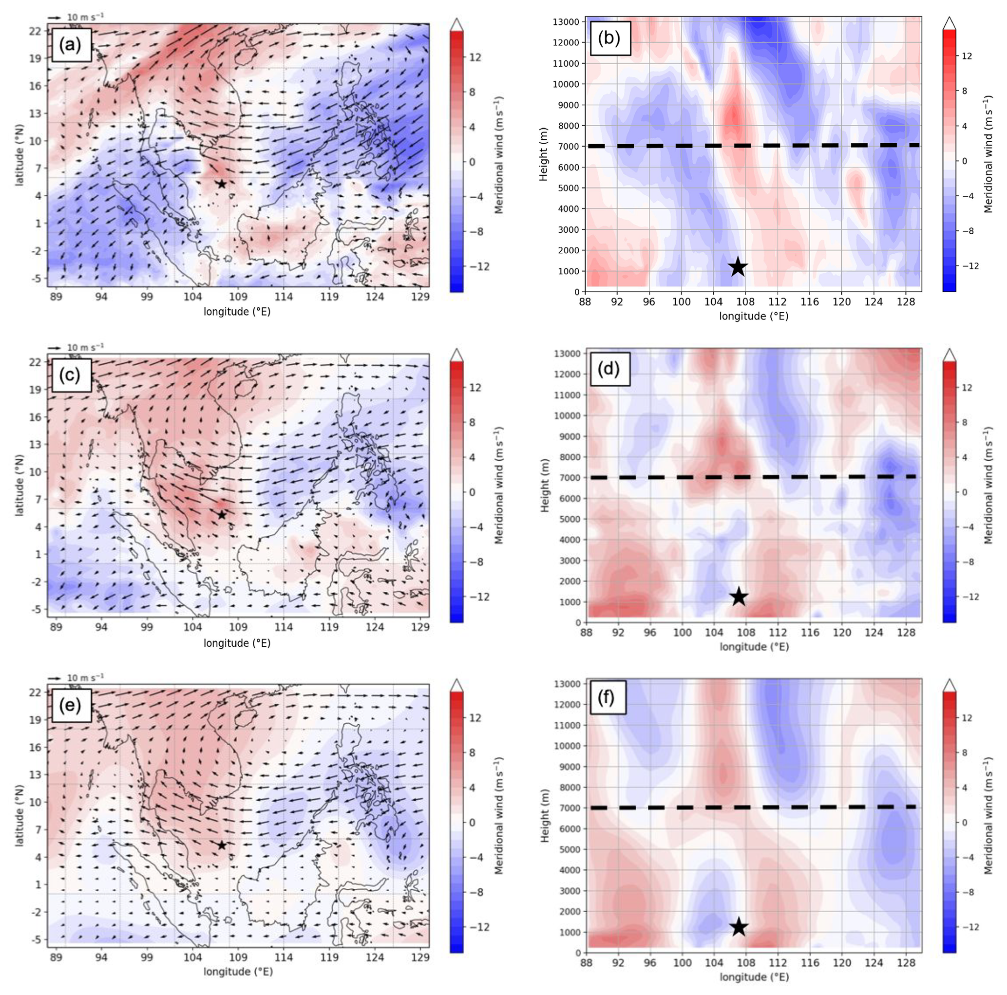
Figure 1(a) Meridional wind (shaded; m s−1) and horizontal wind (m s−1; reference vector = 10 m s−1) at 7 km, from the global MetUM simulation initialised at 12:00 UTC on 21 October 2018, valid at 12:00 UTC on 23 October 2018 (T+48); (b) longitude–height cross-section of meridional wind (shaded; m s−1) along 6∘ N. Overlain are the 850 hPa vorticity centre identified by the tracking algorithm (black star) and the height of the x–y section in (a) (dashed black line at 7 km); (c) and (d), as in (a) and (b) but for the full balanced meridional wind from the SGT tool, , with diabatic forcing; (e) and (f), as in (c) and (d) but for the geostrophic component of the meridional wind, vg, after smoothing and the application of the tropical filter.
Example output from the SGT tool and the driving global MetUM are compared across a much larger domain in Fig. 2 for another event in December 2018, characterised by twin tropical cyclones either side of the Equator over the Indian Ocean. The extratropical horizontal flow (poleward of 20∘ N) is dominated by the SGT balance flow (cf. Fig. 2a and c) including a Rossby wave packet extending eastwards from China and the Korean Peninsula. Figure 2 demonstrates the ability of the SGT tool to partition the 3-D balanced ageostrophic flow into that forced by diabatic heating and geostrophic forcing. Vertical velocity in this northern part of the domain is largely driven by geostrophic forcing (Fig. 2b and f). A notable exception is the ascent ahead of a mid-latitude trough on the west side of Japan which is amplified by heating (Fig. 2d). The unbalanced residual component, vr, which represents the difference between the wind from the MetUM simulation and that output by the SGT tool, highlights the flow features in the MetUM that are not captured by SGT balance flow (Fig. 2e). This term has relatively small amplitude poleward of 20∘ N, except the area near Japan next to the heating already mentioned. However, the meridional component of the unbalanced residual wind, vr, is larger in the tropics and changes sign at about 10∘ S (converging from the north and south at this latitude). Given the time of year, this pattern is likely a signature of the low-level convergence of the Hadley circulation. Note that there are also large zonal flows in the unbalanced residual converging on Sumatra at this time (Fig. 2e). Zonal variation in wind along the Equator cannot be described by SGT balance, including equatorial wave dynamics. The strong circulation around the twin tropical cyclones is only partially represented by the SGT balance, with a smaller unbalanced residual on their poleward flanks and a large residual in between (since the equatorial westerlies between them cannot be part of the SGT balance). Also, the balance is not good nearer the middle of the tropical cyclones because semi-geostrophic balance is inaccurate when trajectory curvature is much tighter than the Rossby radius of deformation. However, later Fig. 10 shows that semi-geostrophic balance can describe qualitatively the rotational flow around the Borneo vortex (except equatorward of about 2–3∘ N) and the vertical motion in balance with latent heating on the synoptic scale.
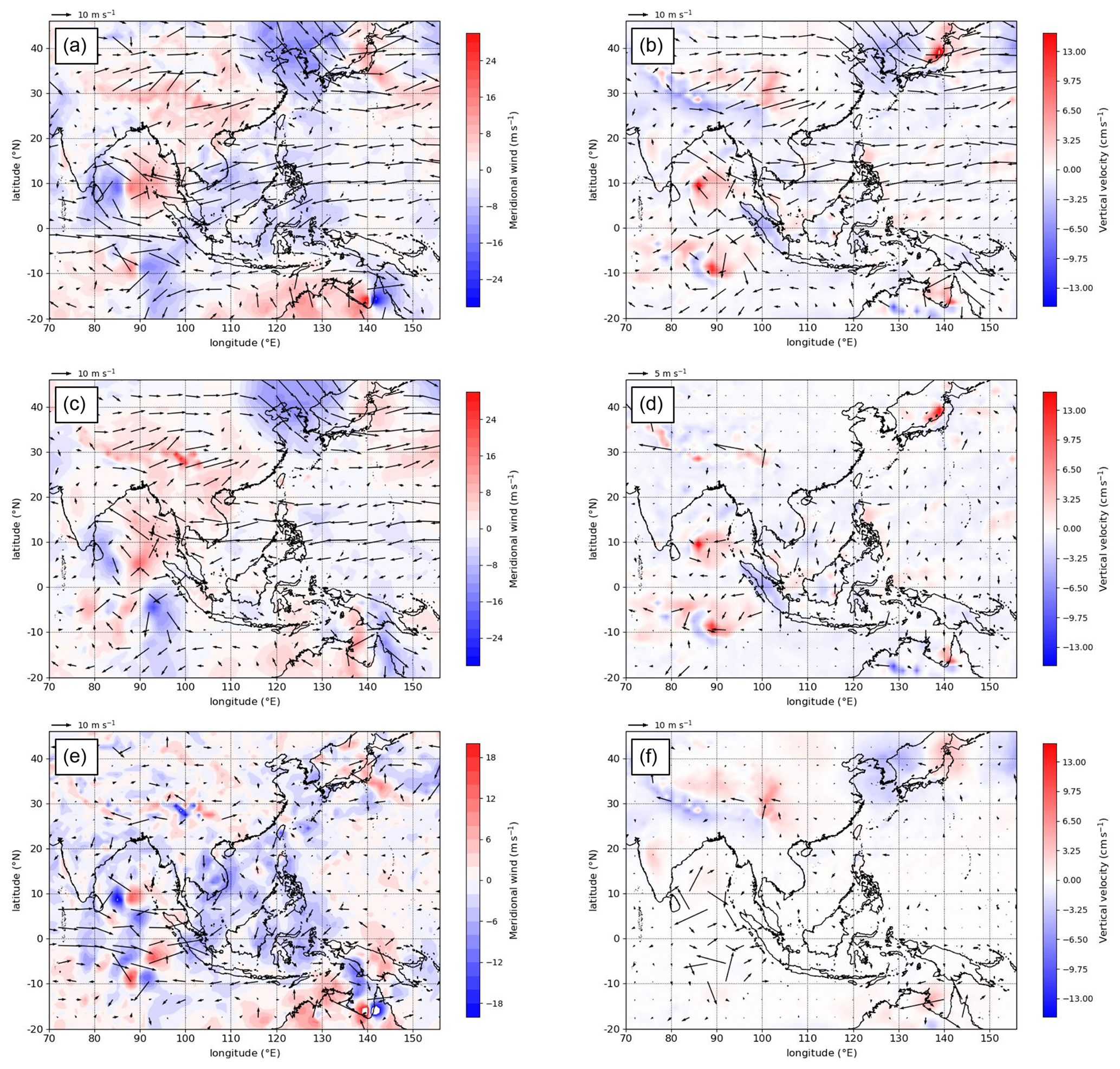
Figure 2(a) Meridional wind (shaded; m s−1) at 2 km from the N768 MetUM simulation initialised at 12:00 UTC on 11 December 2018, valid at 12:00 UTC on 13 December 2018 (T+48). (c) Meridional component of the full balanced wind, , and (e) unbalanced residual meridional wind, vr, at 2 km from the SGT tool at 12:00 UTC on 13 December 2018; (b), (d) and (f) Vertical velocity (shaded; cm s−1) at 2 km inverted from the SGT tool at 12:00 UTC on 13 December 2018 with (b) full forcing, (d) diabatic forcing only, and (f) geostrophic forcing only. The wind vectors represent the full horizontal wind in (a)–(c), the forced ageostrophic component in (d) and (f), and the unbalanced residual component in (e), with the reference vector in the upper left corner for all panels.
2.3 Verification data
To verify the representation of rainfall within the vortex by the MetUM, Integrated Multi-satellitE Retrievals for Global Precipitation Measurement (GPM-IMERG; Huffman et al., 2019) satellite data are analysed. The product used is Level 3 Final Run Precipitation, which combines precipitation estimates from GPM satellites (see https://gpm.nasa.gov/missions/GPM/constellation, last access: 12 October 2023) and Global Precipitation Climatology Centre precipitation rain gauges and has a horizontal grid spacing of 0.1∘ and an output interval of 30 min. The product combines infrared geostationary satellite data with passive microwave radiometer data to produce the best observational precipitation data available in each 30 min interval.
The ERA5 reanalysis dataset (Hersbach and Coauthors, 2020) is used to further verify the ability of the MetUM to represent the 3-D structure of the vortex. The ERA5 dataset has an output interval of 1 h, a spectral horizontal resolution of TL639 (approximately 31 km grid spacing at the Equator), and 137 hybrid sigma–pressure levels in the vertical between the surface and 1 Pa.
2.4 Vortex tracking
The vortex event chosen for analysis herein was identified by tracking 850 hPa relative vorticity at T63 resolution at 6 h intervals in ERA-Interim reanalysis data (Dee and Coauthors, 2011). The dataset was produced as part of the Newton Fund project under the auspices of the WCSSP Southeast Asia project by Dr. Kevin Hodges of the National Centre for Atmospheric Science and Department of Meteorology, University of Reading. The algorithm used to track vortices in this study has been used previously on a range of synoptic-scale and mesoscale vortices including midlatitude cyclones (e.g. Priestley et al., 2020), tropical cyclones (e.g. Manganello and Coauthors, 2016) and polar lows (e.g. Zappa et al., 2014), as well as the Borneo vortex (Liang et al., 2021). In the case of Borneo vortices in this study, disturbances with relative vorticity greater than s−1 that last for more than 1 d during the period October to March are retained.
The Borneo vortex analysed in this article developed to the north of Borneo on 21 October 2018 and tracked westward over the South China Sea, producing heavy rainfall across southern Vietnam and Thailand between 23 and 26 October 2018. The vortex is visible in satellite data as a region of enhanced total precipitable water to the north of Borneo at 06:00 UTC on 22 October 2018 (Fig. 3a). The vortex then moved westward through the South China Sea, located off the southern coast of Vietnam at 06:00 UTC on 23 October 2018 (Fig. 3b), before crossing southern Vietnam and moving into Thailand and northern Peninsular Malaysia on 24 October 2018 (not shown). The two snapshots shown here in Fig. 3a and b closely correspond to the intensifying and maximum intensity stages of the vortex presented later in Figs. 6 and 7, respectively. Although its impact on landfall was not unusually great, this vortex maintained a coherent structure for several days as it tracked westward across the South China Sea, providing a meaningful length of time to study its structure and evolution. To investigate the evolution of the vortex further, the regional and global MetUM simulations are analysed alongside output from the SGT tool, which was driven by the global MetUM simulation as discussed in Sect. 2. All remaining analysis in this paper is directly related to these MetUM simulations and to output from the SGT tool.
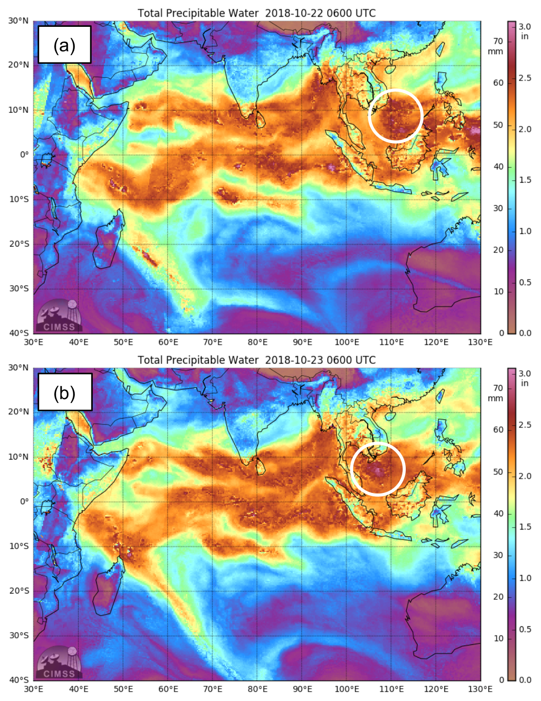
Figure 3Total precipitable water satellite data (shaded, mm) from the Morphed Integrated Microwave Imagery at CIMSS (MIMIC) product, valid at 06:00 UTC on (a) 22 October 2018 and (b) 23 October 2018. The region of enhanced total precipitable water associated with the Borneo vortex is circled in white.
The 12 h accumulated precipitation ending at 12:00 UTC on 23 October 2018 is presented in Fig. 4, for the two MetUM simulations relative to GPM-IMERG precipitation data, alongside Himawari-8 brightness temperature observations valid at 12:00 UTC on 23 October 2018. The vortex, in its mature phase, is centred in the South China Sea near 107∘ E, 5∘ N, and both the IMERG satellite observations and MetUM simulations illustrate that the heaviest and most persistent precipitation is located to the north of the cyclone centre, in agreement with previous observational and modelling studies (Chang et al., 1982; Juneng et al., 2007; Koseki et al., 2014; Liang et al., 2021). The organised, larger region of precipitation extending from the northwest to the northeast of the cyclone centre in the 4.4 km MetUM simulation is reminiscent of the comma-type structure described by Koseki et al. (2014) in their idealised simulation study of a westward-propagating vortex. The brightness temperature field also indicates that the deepest convective clouds are concentrated to the north of the cyclone centre (Fig. 4d). Appendix B discusses the vortex structure 24 h later at 12:00 UTC on 24 October 2018, as the vortex entered its weakening phase. For reference, the entire westward track of the vortex between 12:00 UTC on 21 October and 12:00 UTC on 26 October is overlaid on Figs. 4b and B1b, with the centre position marked every 12 h.
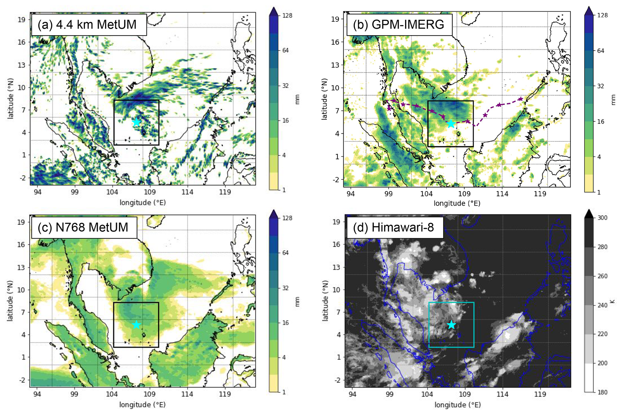
Figure 4The 12 h accumulated precipitation ending at 12:00 UTC on 23 October 2018 (shaded, mm) from (a) 4.4 km MetUM simulation initialised at 12:00 UTC on 21 October 2018, (b) GPM-IMERG satellite product, (c) N768 MetUM simulation initialised at 12:00 UTC on 21 October 2018. (d) Brightness temperature (shaded, K) from the Himawari-8 satellite, valid at 12:00 UTC on 23 October 2018. The cyan star marks the position of the Borneo vortex centre. The dashed purple line in (b) represents the vortex track between 12:00 UTC on 21 October and 12:00 UTC on 26 October 2018, with the smaller purple stars marking the vortex centre position every 12 h.
Circulation expressed as area-averaged relative vorticity and 12 h accumulated precipitation, in a box with radius 3∘ following and centred on the vortex, summarise the cyclone's life cycle and capture the intensifying, mature and weakening phases (Fig. 5). The vortex is present in ERA5 reanalysis data at 12:00 UTC on 21 October 2018, when the 4.4 km and global MetUM simulations are initialised, before intensifying as it moves westward over the next 48 h, as shown by the increase in area-averaged relative vorticity (Fig. 5a). Both simulations capture the increase and subsequent peak in vorticity during this time, although the simulated vortex reaches its mature phase, characterised by maximum strength, 12 h later than indicated in the reanalysis. All three datasets then capture the gradual weakening of the vortex from 24 October 2018 onward, as it moves further west to make landfall in Thailand. The 12 h accumulated precipitation demonstrates a pronounced diurnal cycle (Fig. 5b), with the heaviest precipitation accompanying the vortex occurring during local day time (in the 12 h ending at 19:00 LT). The 4.4 km simulation shows good quantitative agreement with IMERG observations for the first 48 h up to 12:00 UTC on 23 October 2018, before the datasets diverge somewhat. The global simulation is unable to capture this diurnal cycle, with the largest accumulated precipitation totals sometimes occurring during local night time, as on 23 October 2018. This discrepancy of the global model, relative to IMERG and the 4.4 km simulation, is likely due to the model's use of a convective parameterisation scheme, which is unable to accurately represent the physical processes linked to the observed diurnal cycle of convection (e.g. Love et al., 2011; Birch et al., 2016).
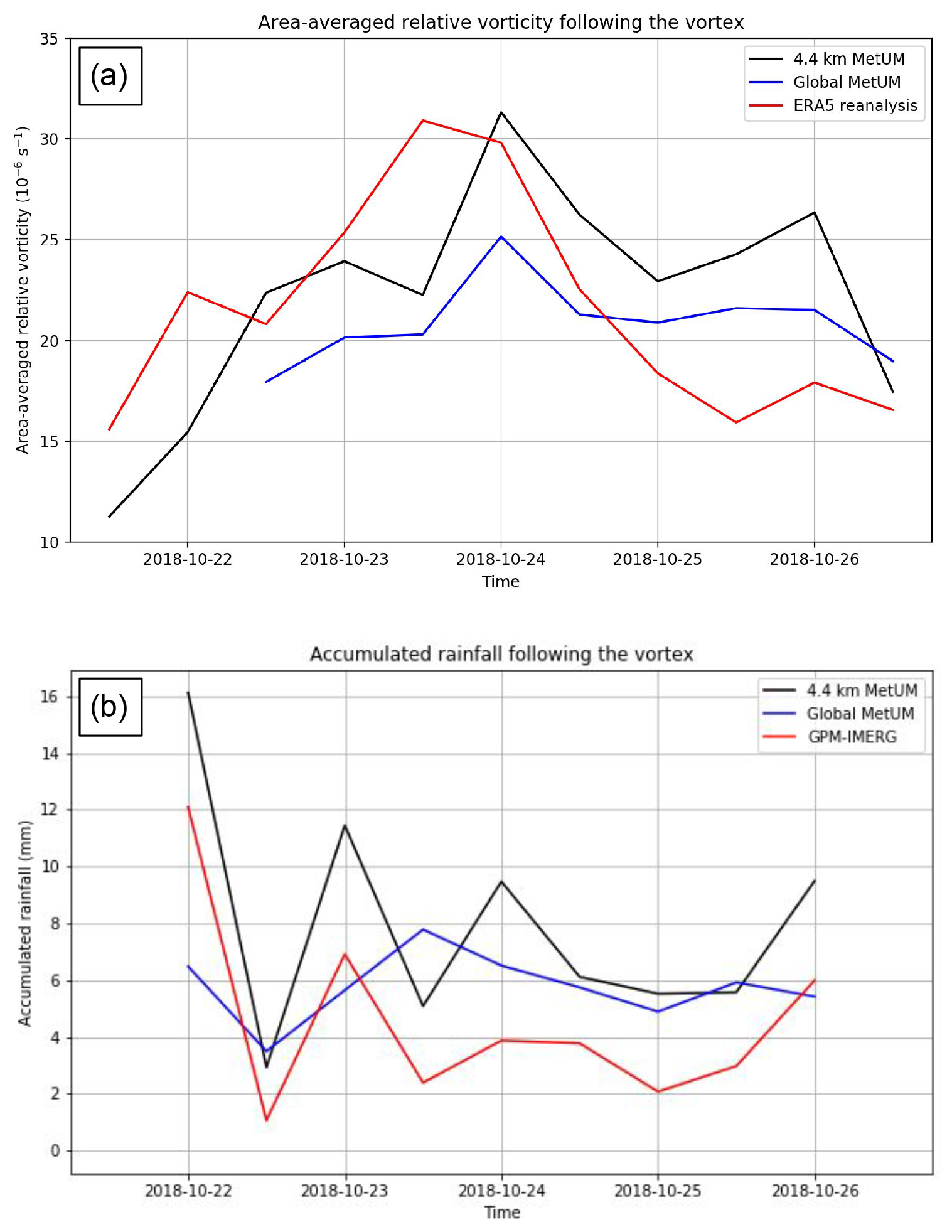
Figure 5(a) Area-averaged relative vorticity in a 3∘ box following and centred on the vortex from the 4.4 km MetUM simulation (black line), the N768 MetUM simulation (blue line) and the ERA5 reanalysis product (red line). Area-averaged relative vorticity is calculated at 850 hPa in the 4.4 km MetUM simulation and ERA5 reanalysis, and at the nearest model level at 1.4 km altitude for the N768 simulation due to the unavailability of appropriate pressure level data. (b) The 12 h accumulated precipitation in a 3∘ box following and centred on the vortex, from the 4.4 km MetUM simulation (black line), the N768 MetUM simulation (blue line) and the GPM-IMERG satellite product (red line).
The westward progression of the vortex across the South China Sea in the 4.4 km MetUM simulation is illustrated in Figs. 6 to 8. At 12:00 UTC on 22 October 2018, the vortex is in its intensification phase (see Fig. 5a) and is centred off the northwestern coast of Borneo, with a cyclonic circulation evident in the 850 hPa meridional wind field (v), although the southward component is much stronger than the northward component (Fig. 6a). The vertical cross-section indicates that the vortex tilts westward with height at this time and is not purely confined to the lower troposphere as suggested in some previous studies (Trilaksono et al., 2012; Liang et al., 2021), with a dipole in v extending to around 350 hPa (Fig. 6b). The Borneo vortex is embedded within a region of enhanced column water vapour that extends westwards across the central Philippines and through the South China Sea reaching into southeastern Vietnam at this time (Fig. 6c). In contrast, much drier air is located ahead of the moist air (103–107∘ E) and in the northeasterly flow crossing the northern Philippines and into central Vietnam, impinging on the northern flank of the moist region. The low-level vortex signature in relative humidity is weak, but the extensive region of relative humidity close to 100 % in the mid to upper troposphere is collocated with northward flow in v and is suggestive of the presence of mid-level to deep convection (Fig. 6d).
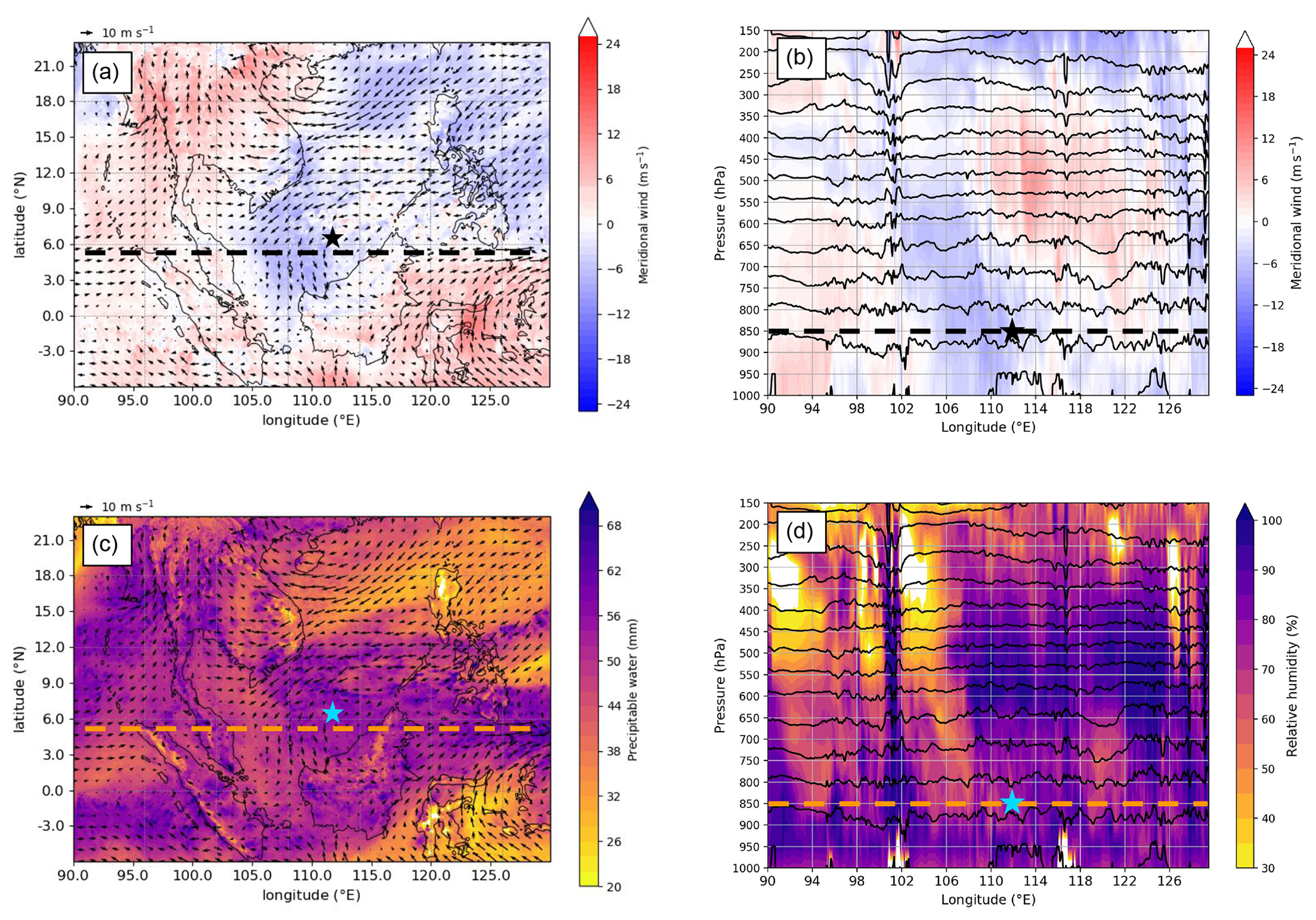
Figure 6(a) Borneo vortex at intensifying stage. Meridional wind (shaded; m s−1) and horizontal wind vectors (m s−1; reference vector = 10 m s−1) at 850 hPa from the 4.4 km MetUM simulation initialised at 12:00 UTC on 21 October 2018, valid at 12:00 UTC on 22 October 2018 (T+24); (b) longitude–height cross-section of meridional wind (shaded; m s−1) with potential temperature overlaid (black contours; every 2 K), from the same 4.4 km MetUM simulation. (c) as in (a), but for total precipitable water (shaded; mm); (d) as in (b), but for relative humidity (shaded; %). Overlaid is the 850 hPa vorticity centre identified by the tracking algorithm (black/blue star).
The vortex circulation and its associated region of moist, unstable air moves west through the South China Sea over the following 48 h, located several hundred kilometres south of Vietnam at 12:00 UTC on 23 October 2018 (Fig. 7) and between southern Vietnam and Peninsular Malaysia at 12:00 UTC on 24 October 2018 (Fig. 8). At the time of maximum intensity, there is some indication that the isentropic surfaces dome slightly in the lower-tropospheric vortex (on the scale of the vortex), as expected from thermal wind balance in the presence of a warm core structure (Fig. 7b and d). Generally, however, isentropic surfaces are almost flat and static stability reasonably uniform, as expected in the tropics (e.g. Vallis, 2017), aside from small-scale perturbations due to deep convection, which is explicit in the 4.4 km MetUM simulation. Small-scale perturbations in potential temperature (θ) likely associated with convective updraughts and collocated with relative humidity close to 100 % are seen near 107∘ E at the time of maximum vortex intensity (Fig. 7d) and at 106∘ E at the start of the weakening phase (Fig. 8d).
The low-level vortex circulation becomes stronger and more coherent between 12:00 UTC on 22 and 23 October 2018, coincident with the increase in circulation in the ERA5 reanalysis as the vortex moves from its intensifying phase into its mature phase (cf. Figs. 5a, 6a and 7a). Just 24 h later at 12:00 UTC on 24 October 2018, the vortex is approaching its weakening phase (see Fig. 5a). During this period, drier air to the northeast and southeast of the vortex at 850 hPa progressively encroaches from the east (Figs. 7c and 8c). The westward vertical tilt of the vortex, as approximated by the longitudinal spacing between the 850 hPa vortex identified by the tracking algorithm and the leading edge of the north–south dipole in v at 500 hPa, slowly increases during this time (Figs. 6b, 7b and 8b), suggesting that the vortex may comprise a low-level vortex and a mid-level wave moving at different speeds. A coherent, westward-moving region of cyclonic relative vorticity and relative humidity values near 100 % between 400 and 600 hPa suggests that this mid-level wave is associated with organised deep convection (Figs. 6d, 7d and 8d). This hypothesis will be tested in Sect. 5 by analysing output from the SGT balance approximation tool.
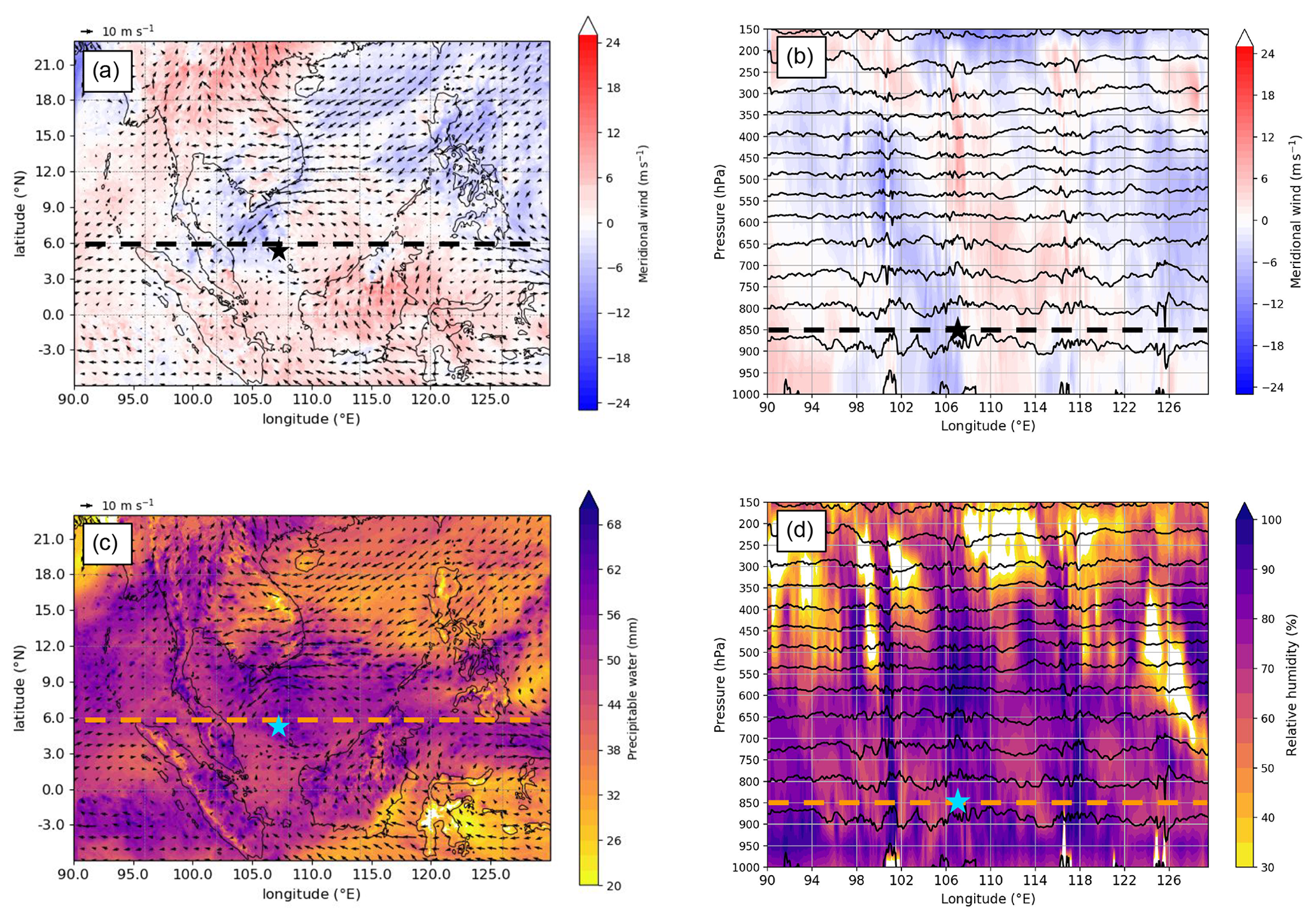
Figure 7Borneo vortex at maximum intensity (mature stage). As in Fig. 6 but valid at 12:00 UTC on 23 October 2018 (T+48).
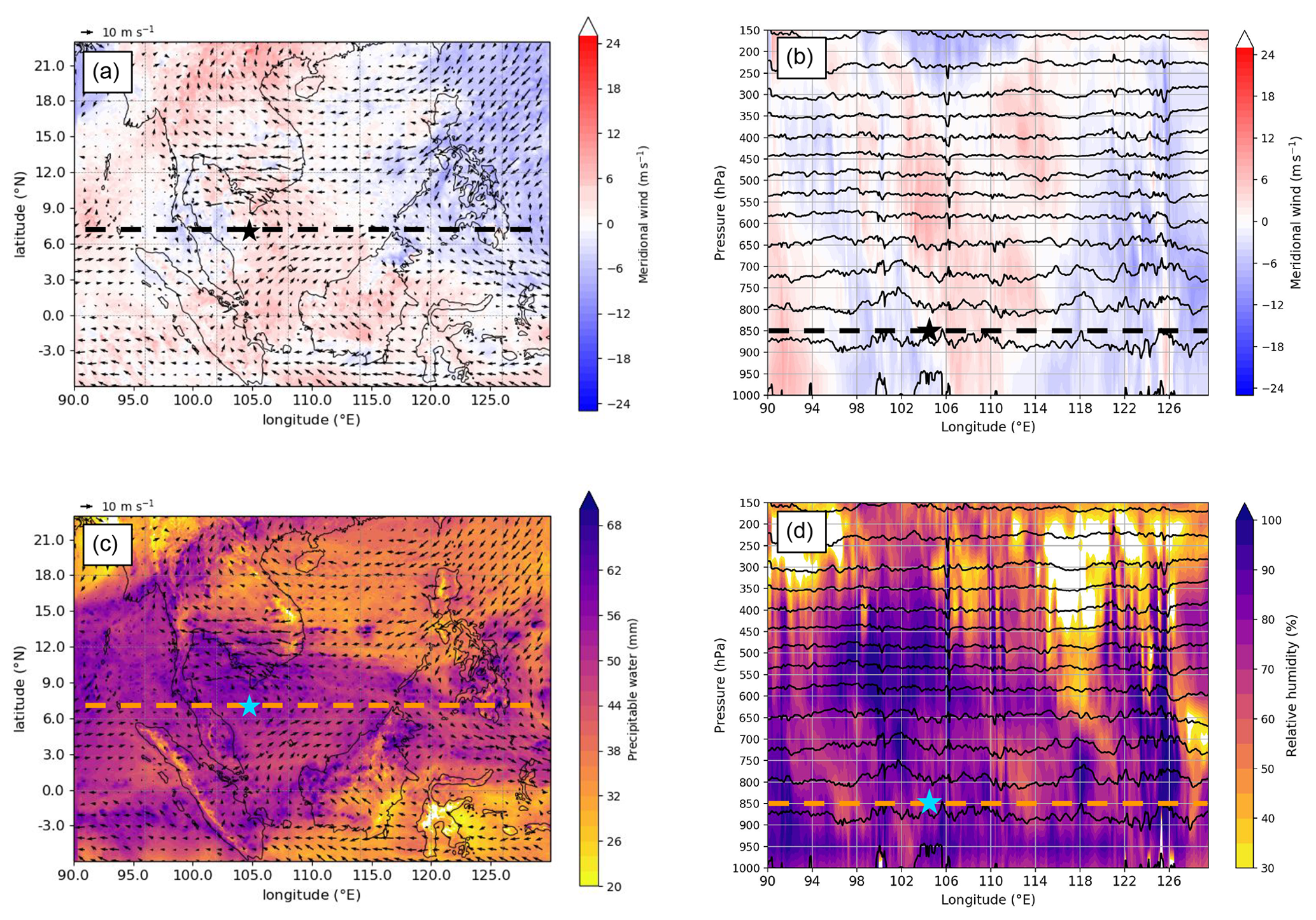
Figure 8Borneo vortex at start of weakening phase. As in Fig. 6 but valid at 12:00 UTC on 24 October 2018 (T+72).
5.1 Three-dimensional Borneo vortex structure
As discussed in Sect. 2.2, a key purpose of the SGT balance approximation tool is that it enables investigation of the degree to which the vortex can be understood in terms of balanced dynamics and the role of diabatic heating in the structure, intensification and maintenance of the vortex.
When considering 3-D vortex structure and movement, it is important to characterise the large-scale flow. The vertical and horizontal shear in the background zonal flow are crucial ingredients, affecting system tilt and possible growth mechanisms. The mean flow during the case study (12:00 UTC on 21 October to 12:00 UTC on 26 October 2018) is generally easterly, when averaged over a longitude band covering the region of interest (Fig. 9a). Easterlies strengthen with height up to around 7 km, with a weaker gradient above this height. At 7 km, there is a broad maximum in easterly flow across 8–11∘ N. There is a strong cyclonic shear on the southern flank of the easterlies across 5–7∘ N. This easterly flow pattern is typical of the northeast winter monsoon (e.g. Chang et al., 2005a).
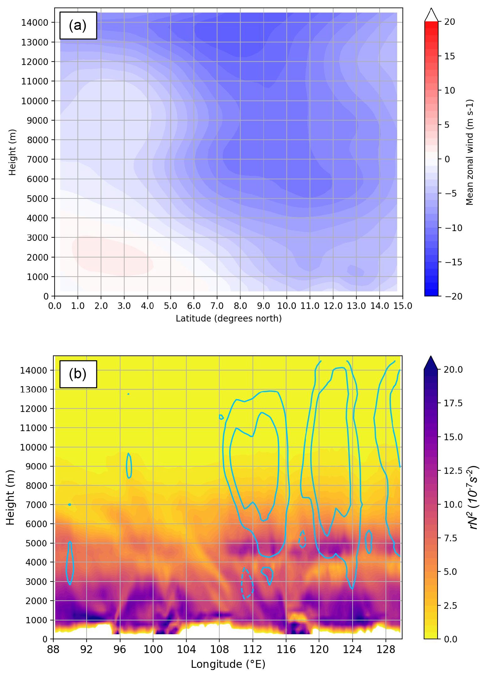
Figure 9(a) Mean zonal wind from the N768 MetUM simulation initialised at 12:00 UTC on 21 October 2018, averaged over time (12:00 UTC on 21 October to 12:00 UTC on 26 October 2018) and longitude (95 to 120∘ E). (b) The quantity rN2 (shaded; 10−7 s−2), averaged across 5.5–7∘ N, combines specific humidity and static stability to identify changes between moist air with high static stability (large rN2) and drier air (smaller rN2), valid at 00:00 UTC on 22 October 2018 (T+12). Blue contours indicate the diabatically forced component of the balanced vertical velocity from the SGT tool (−2, 2, 6, 10 cm s−1).
A second key ingredient of the basic state is stability. Colour shading in Fig. 9b shows rN2, the specific humidity multiplied by the static stability, . It the next section it will be shown that the vertical gradient in this quantity can define a moist stability interface along which “diabatic Rossby waves” (e.g. Parker and Thorpe, 1995; Moore and Montgomery, 2004; Boettcher and Wernli, 2013) can propagate. The pale-blue contours show the diabatically forced vertical motion, wdiab, consistent with balanced motion deduced using the SGT tool. There is an obvious wave at the level of the strong gradient in rN2 (4.5–5 km) and above. It is important that the moist stability interface occurs within the region of large-scale vertical shear, given that this vertical shear enables baroclinic interaction between the low-level vortex and mid-level wave.
In Fig. 10, the vertical velocity (w, shown at 7 km) and the horizontal wind vectors (shown at 2 km) are partitioned into the balanced flow response to diabatic heating () and geostrophic forcing using the SGT tool, valid at 12:00 UTC on 23 October (T+48 in the driving global MetUM simulation) when the vortex circulation peaks in ERA5 (Fig. 5b). The qualitative similarity between w from the SGT tool and the 1 h accumulated heating from the driving global MetUM (Fig. 10a) shows that the regions of ascent identified by the SGT tool are representative of the flow in the MetUM, given that on scales larger than several hundred kilometres the primary balance in the thermodynamic equation in the tropics is between diabatic heating and vertical motion multiplied by static stability (as expressed in Eq. 2). The coherent region of heating to the south of Vietnam on the northwestern flank of the cyclonic circulation at 2 km is collocated with the maximum in total precipitable water and the area of organised precipitation associated with the vortex at this time (cf. Figs. 4c and 10a). An organised region of ascent is located in a similar region relative to the 2 km cyclonic circulation in the balanced flow from the SGT tool (Fig. 10b). This qualitative similarity indicates that the vortex is described by the balanced flow. Examining the partition of 3-D ageostrophic motion into that forced by (Fig. 10c) and large-scale geostrophic forcing (Fig. 10d) reveals that upward motion within the vortex is primarily forced by . The 2 km ageostrophic wind vectors in Fig. 10c converge from the southwest and northeast underneath the heating in an asymmetric pattern, with the main inflow from the equatorward side. In contrast, the large-scale geostrophic forcing produces an anticyclonic circulation that opposes the geostrophic wind (Fig. 10d), although the difference in vector scaling should be noted. This result implies that the full flow is sub-geostrophic.
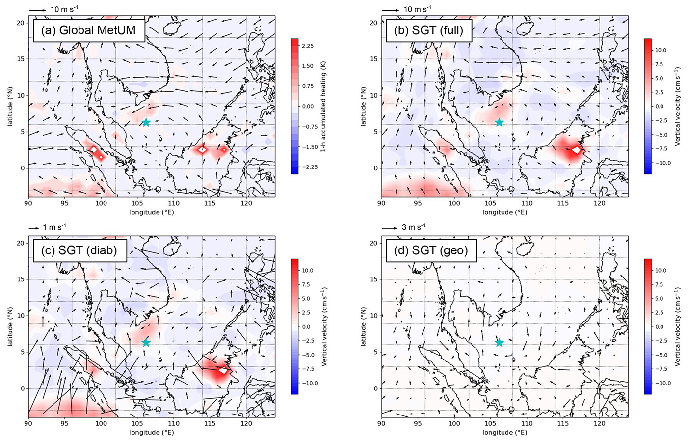
Figure 10(a) The 1 h accumulated heating at 7 km (shaded; K) and horizontal wind at 2 km (vectors; m s−1) from N768 MetUM simulation initialised at 12:00 UTC on 21 October 2018, valid at 12:00 UTC on 23 October 2018 (T+48). (b–d) Balanced vertical velocity at 7 km (shaded; cm s−1) and horizontal wind at 2 km (vectors; m s−1) inverted using the SGT tool at 12:00 UTC on 23 October 2018 with (b) full forcing, (c) diabatic forcing only, and (d) geostrophic forcing only. In (a) and (b), the wind vectors represent the full horizontal wind. In (c) and (d), the wind vectors represent the ageostrophic wind only. Note that the scale of the vectors is different in all panels, with the key in the upper left corner.
The time sequence of wave propagation is shown in Fig. 11 over a 2 d interval. The wave grows to significant amplitude and therefore develops into pronounced meridional undulation in the eastward flow. The southward–northward velocity dipole moves westward together with the 7 km PV and wdiab maxima, the locations of which are marked onto the figure panels using symbols. The easterlies at 7 km also extend westwards with the wave. The vertical cross-sections are calculated along 6∘ N. The asterisk just above the boundary layer (at 1.4 km) shows the diagnosed location of the vortex centre, and this centre is also marked on the 7 km maps. The PV maximum is close to the zero node of v, as expected for Rossby wave propagation, and at most times the maximum in wdiab is slightly shifted to the west. The upper-level wave propagates faster to the west than the lower-level vortex – this property will be explained in Sect. 5.3. Also, note how v is partitioned into two distinct layers, split approximately at 3–4 km. The vortex circulation is confined below this level and is approximately untilted up to 3 km a.s.l.
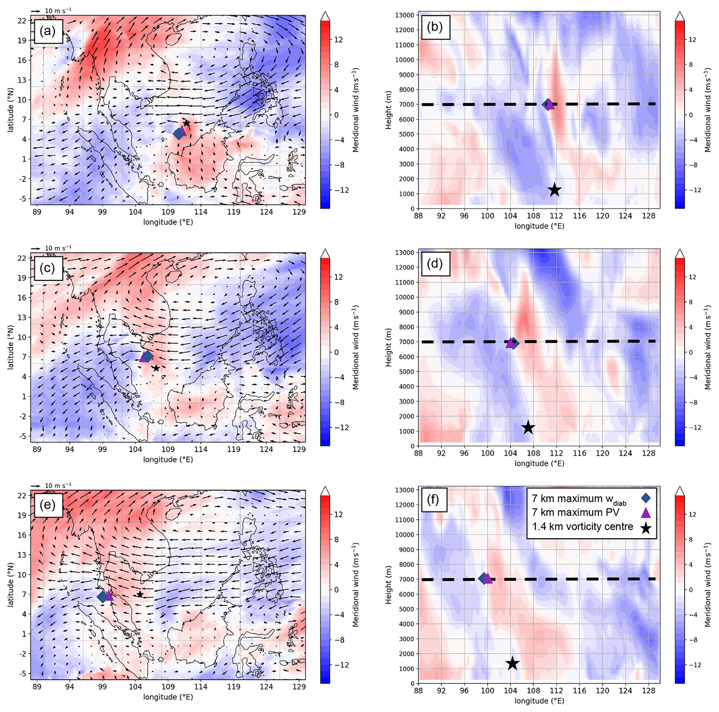
Figure 11(a) Meridional wind (shaded; m s−1) and horizontal wind (m s−1; reference vector = 10 m s−1) at 7 km, from the global MetUM simulation initialised at 12:00 UTC on 21 October 2018, valid at 12:00 UTC on 22 October 2018 (T+24); (b) longitude–height cross-section of meridional wind (shaded; m s−1) along 6∘ N. Overlain are the 850 hPa vorticity centre identified by the tracking algorithm (black star), maximum PV at 7 km from the MetUM simulation (purple triangle), maximum vertical velocity forced by diabatic heating from the SGT tool at 7 km (blue diamond), and the height of the x–y section in (a) (dashed black line at 7 km); (c) and (d), as in (a) and (b) but valid at 12:00 UTC on 23 October 2018 (T+48); (e) and (f), as in (a) and (b) but valid at 12:00 UTC on 24 October 2018 (T+72). For reference, panels (c) and (d) are equivalent to Fig. 1a and b.
Figure 12c and d show the horizontal flow at 7 km in the earliest stages of the low-level vortex development (cf. Fig. 5a); the asterisk marks the vorticity centre diagnosed using the tracking algorithm. Note how the centre is situated on the southern flank of the strong easterlies of a subtropical anticyclone and associated with an easterly cold surge event. Within the shear zone between 4–7∘ N, a well-defined wave has developed in both the v and balanced w components, as well as in Ertel PV. This structure is even more apparent in vertical cross-sections along 6∘ N in Fig. 12a and b. At this time, the signature in v is strongest in the layer 4–9 km, upwards from the moist stability interface at about 5 km, but with some signature extending downwards too. The signature in balanced wdiab is stronger at higher levels than in v, reflecting the extension of the latent heating in deep convection into the upper troposphere. As characteristic of a Rossby wave, relative vorticity has to be in quadrature with v and so are the PV anomalies at 7 km (this analysis level is chosen between the height of the moist stability interface, at 5 km, and maximum wdiab, at 9 km). The positive wdiab maxima are shifted westwards relative to the positive vorticity maxima into the southerly sectors of the wave. This structure means that typically the ascent leads the positive PV anomalies in the propagation of the wave westwards. As explained in the next section, this structure is a key signature of diabatic Rossby wave propagation in the mid-troposphere.
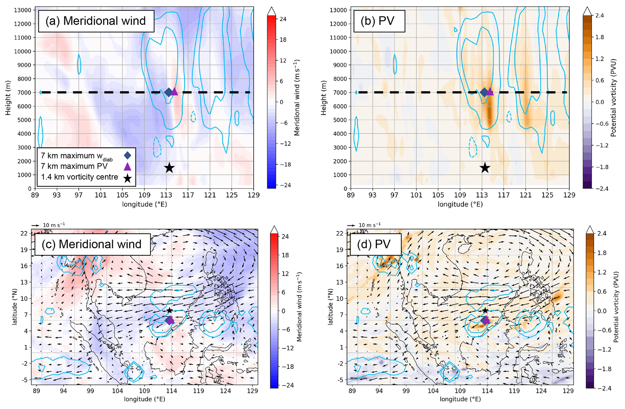
Figure 12(a) Longitude–height cross-sections of meridional wind (shaded; m s−1), and (b) Ertel PV (shaded; PVU) along 6∘ N, from the global MetUM simulation initialised at 12:00 UTC on 21 October 2018, valid at 00:00 UTC on 22 October 2018 (T+12). (c) Meridional wind (shaded; m s−1) and (d) Ertel PV (shaded; PVU) with horizontal wind vectors overlaid (m s−1; reference vector = 10 m s−1) at 7 km. In all panels, balanced vertical velocity forced by diabatic heating is overlain (blue contours; −2, 2, 6 and 10 cm s−1).
5.2 Theory for diabatic Rossby wave propagation
Diagnosis of the MetUM simulations above has shown that a westward-propagating wave-like disturbance exists with a coherent signature in v, as well as Ertel PV and w in the mid-troposphere, and θ near the lower boundary. Here, following Bretherton (1966) and Hoskins et al. (1985), we will describe any such wave in PV as a “Rossby wave”. This formulation includes waves that exist on a basic state (here sector zonal average) meridional PV gradient or θ gradient at the lower boundary. The common feature is that the propagation mechanism relies on meridional advection of PV (or lower boundary θ) and the meridional flows that the chain of PV (or θ) anomalies induces. Hoskins et al. (1985) argue that the propagation direction of a wave and the nature of its interaction with a second wave at different level (mutual growth or decay) can be anticipated without explicit calculation of the flows induced by each wave using a specific form of balance or PV inversion relation. All that is required from balance is that v induced by one wave is in quadrature with PV. Then, the sense of propagation and interaction depends only on the phase difference between variables and also between a pair of waves. Heifetz et al. (2004) derived evolution equations for the amplitude and phase of such counter-propagating Rossby waves (CRWs) that can provide a mechanistic explanation for baroclinic instability. De Vries et al. (2010) extended the framework to moist dynamics by parameterising in terms of w and then using the omega equation to relate induced w to PV in the waves. Following other authors (e.g. Moore and Montgomery, 2004; Boettcher and Wernli, 2013) the term “diabatic Rossby wave” was used to describe PV waves where the zonal propagation is dependent on the coupling with w and latent heat release. The argument for propagation is similar but depends on the phase of induced w rather than v (or a combination of both). Here we will use this CRW approach to analyse the output from the MetUM and understand whether the zonal phase speeds of the waves are consistent with the propagation mechanism and the role of latent heating in the waves.
Begin with the Ertel PV equation linearised about a basic state zonal flow, including the effects of :
where q is perturbation Ertel PV and ζ is the vertical component of basic state absolute vorticity. U(y,z), Q(y,z) and ρr(z) are the basic state zonal flow, PV and density, respectively. Note that the PV is materially conserved following the full flow in the absence of heating, including vertical advection, a major difference from quasi-geostrophic theory where only horizontal advection by the geostrophic flow is considered. Here we will take the approach that, although the balance approximation is not known precisely, Eq. (4) describes the evolution of the flow, where v and w are understood as the anomalous winds induced by the PV waves. The SGT tool has also been used to show that the signature of the balanced semi-geostrophic wind is indeed similar to that of the full wind in the MetUM and is the justification for the analysis. This result enables application of PV thinking and the CRW approach, where the propagation rates of the waves can be estimated and also attributed to the effects of and the conditions for growth or decay through wave interaction can be deduced simply from phase differences between waves.
De Vries et al. (2010) investigate two types of closure in the parameterisation of heating: “large-scale rain” and wave-CISK (Conditional Instability of the Second Kind), which differ in the assumed relationship between and w. Here, the large-scale rain approach is used, in which the heating rate is proportional to the product of basic state specific humidity, r, and w at each location (no meridional variation is assumed for simplicity):
This approximation is motivated by the ascent of saturated air masses where condensation results in latent heat release. Note that the typical balance of the thermodynamic equation in the tropics is between large-scale w and , in which case ϵr≈1. However, when there is also geostrophic forcing of w, this parameterisation is only valid for ϵr<1 at all levels. It is typical to take ϵ to be a constant. Linearisation of the dynamics requires that there is a symmetric cooling where there is descent; this requirement is partly justified by arguing that there is enhanced long-wave cooling from clear air regions. If it can be assumed that rN2 varies more quickly in the vertical than w does at a level that we will call a “moist stability interface” (see Fig. 9b), so that w can be taken outside the heating gradient , then Eq. (4) becomes
where encapsulates the basic state moist stability gradient that the diabatic PV wave propagates along as a result of the gradient in heating coupled with w. Together with the equation for the evolution of θ on the lower boundary, Eq. (4) completely specifies the balanced evolution because the PV can be inverted to obtain the balanced wind field at any instant. Appendix A shows how the CRW theory can be used to deduce expressions for the zonal phase speed of a PV wave at upper levels (labelled wave-2 with induced velocity amplitude v2, w2) and a wave in θ along the lower boundary (wave-1 with velocity v1, w1):
The zonal wavelength is , A2 represents the upper wave amplitude in terms of Ertel PV and A1 the lower wave amplitude in θ. The phase speed involves advection by the basic state zonal flow at the level where the wave activity is concentrated for each CRW. The upper CRW propagates relative to the zonal flow, U2, through a mechanism associated with the effect of w and associated heating in the presence of the moist stability gradient (seen in Fig. 9b between 4 and 5 km) as well as meridional advection of the basic state meridional PV gradient, Qy, and vertical advection of the vertical PV gradient, Qz. In the case examined, G is positive and therefore contributes to propagation of the wave to the west, adding to the advection which is also towards the west (U2<0). represents the modification of the phase speed of CRW-2 associated with interaction with v1 and w1 induced by CRW-1 at the level of CRW-2.
The lower CRW propagates against the zonal flow, U1, through meridional advection of the basic state meridional θ gradient, Θy, and the interaction with the upper CRW, represented by . The condition w=0 at the lower boundary is used here. Heifetz et al. (2004) have shown that in a growing normal-mode phase-locked configuration the definition of the CRW structures is such that , although in general initial value problems this relation will not hold. These interaction terms are expected to be smaller than the self-propagation rates.
The self-propagation rate of the diabatic Rossby wave along the moist stability interface (zone of sharp vertical gradient in rN2) can be calculated as
where r(z) and N(z) are the background specific humidity and static stability profiles, evaluated in an upper layer (U) and lower layer (L) separated by an interface zone with a characteristic depth, Δz, and θ separation, Δθ. This factor represents the strength of the basic state interface in terms of the contrast in moist stratification that the wave propagates along. The stronger the contrast, the faster the propagation. The basic state absolute vorticity is calculated from f−Uy. The final component is the amplitude of the wave in the non-dimensionalised diabatic heating rate, , which is assumed proportional to the vertical velocity, w2, in balance with the diabatic Rossby wave motion. This amplitude is estimated from the heating rate represented on scales resolved by the global MetUM; the SGT tool shows that the balanced response to heating dominates the balanced w in the tropics, as expected from scale analysis of the thermodynamic equation. Note that for the lower boundary thermal wave, the amplitude A1 is measured in terms of θ anomalies, and the model level at approximately 1.4 km is used to represent the anomalies and basic state meridional gradient (just above the boundary layer).
5.3 Estimate of zonal propagation rates and baroclinic interaction
Tracking the cyclonic vorticity centres at the upper and lower levels (Fig. 11), the propagation rate of the upper wave is 5–6∘ d−1 (6–8 m s−1) westward. The lower wave and Borneo vortex propagate more slowly: at about 4–5∘ d−1 (5–6 m s−1) from 22 to 23 October and 2∘ d−1 (2.6 m s−1) from 23 to 24 October. The theory shows that the movement of the waves is a combination of advection by the basic state zonal flow, self-propagation and a change in propagation rate through interaction between the waves (Eq. 7). The basic state is estimated by averaging over a domain along the strip of wave activity: 5.5–7.0∘ N and 104–115∘ E, and also averaging over the 5 d time window between 12:00 UTC on 21 and 26 October 2018. This calculation gives basic state zonal flows s−1 and s−1, estimated at 4.5–5.0 km (the level of the moist stability interface in Fig. 9) and 1.4 km respectively. Changing the latitude extent by 1∘ or the time average or length of longitude strip (e.g. 104–120∘ E) gives a variation in these estimates of about ±0.5 m s−1 for U2 and ±0.3 m s−1 for U1.
The self-propagation rate of the lower θ wave relative to the basic state shear can be estimated approximately using Eq. (7). The chief difficulty is estimating the meridional velocity v1 attributable to the lower wave. However, since the flow induced by the upper wave is expected to be much weaker than the flow induced by the lower wave near the lower boundary (Heifetz et al., 2004), the amplitude of the induced flow is estimated from the standard deviation of v over the strip (defined as above) at 1.4 km. Similarly, the wave amplitude A1 is estimated from the standard deviation of the θ perturbation at the same level. The zonal wavelength is approximately 900 km, and the basic state meridional θ gradient in this region is a positive, but weak, K km−1. This calculation yields a propagation rate of 1.5–1.6 m s−1 westwards, adding to advection by U1 to give a phase speed of 2.4–2.7 m s−1 westwards, consistent with the wave movement observed in the later period.
The self-propagation rate of the upper diabatic Rossby wave is harder to estimate. Equation (8) can be used to estimate the magnitude of the propagation rate associated with heating in a sheared environment on the moist stability interface. The basic state moist stability term in Eq. (8) is calculated using 2–4 km to define the lower layer and 6–10 km for the upper layer specific humidity and static stability. The quantities and are given by the average of upper and lower layer values. The moist stability interface depth is Δz=2 km and Δθ=27 K. The zonal wavelength is 900 km, as for the lower wave. The upper wave amplitude in Ertel PV, A2, is estimated from the standard deviation of PV in the strip domain at 7 km. The wave amplitude in heating rate is estimated from the standard deviation of the diabatic temperature tendency (both convection and large-scale rain parameterisation in the MetUM) also at 7 km. Bringing all these terms together the self-propagation rate is 1.3–1.7 m s−1 westwards. Averaged over the same strip at 7 km, the meridional PV gradient is negative (being in the region between the strong easterlies of the cold surge and the cyclonic vorticity strip on its southern edge) with estimated in SI units and v2≈3.4 m s−1, yielding an eastwards contribution to propagation of 0.9 m s−1. The vertical PV gradient term involving Qz is not very coherent and has not been estimated. In contrast, G and Θy are positive over the whole domain of interest, meaning that propagation rate associated with both of these terms is negative definite (westwards), while the Qy term is weak and eastwards. Taking all terms together yields a total phase speed of 7.2–8.4 m s−1 westwards, slightly faster than the observed movement. Note that the cyclonic vorticity strip and upper wave exist 1 d or so before the lower wave and Borneo vortex, so it is possible that the upper wave arises first through barotropic instability of this vorticity strip.
In summary, the self-propagation rates of both waves are considerably weaker than the shear in the background zonal flow, and the propagation through interaction () must be smaller still. So even if the configuration of the waves were favourable, they would not be able to stay phase-locked and must shear apart. However, over the early stages of development the observed difference in wave phase speeds is only 1–3 m s−1, and therefore the estimates of propagation rates from theory are comparable. These self-propagation speeds (1.3–1.7 m s−1) provide an upper bound on the strength of baroclinic interaction between the waves (Heifetz et al., 2004), and gives a growth timescale of 1–1.5 d. Therefore, although the strength of baroclinic interaction is relatively weak compared with the shear rate, baroclinic interaction is a plausible explanation for the emergence of the lower wave and Borneo vortex.
In this paper, the 3-D structure and intensification mechanisms of a Borneo vortex that impacted Vietnam and Thailand in late October 2018 were investigated using Met Office Unified Model (MetUM) simulations and an idealised balance approximation tool. Microwave satellite observations and a MetUM simulation with 4.4 km grid, initialised at 12:00 UTC on 21 October 2018, revealed that the westward-moving vortex was characterised by a coherent maximum in total column water and by a comma-shaped precipitation structure with the heaviest rainfall to the north and northwest of the cyclonic centre, similar to previously documented Borneo vortices.
More detailed analysis of 4.4 km and global MetUM simulations showed that the Borneo vortex tilted westward with height and comprised a low-level closed circulation and a faster-moving mid-level wave that propagated westwards along a vertical gradient in moist stability (specific humidity × static stability) at 4.5 to 5 km. The mid-level wave was characterised by a coherent signature in the meridional wind, PV and vertical velocity fields deduced from semi-geostrophic balance. The large-scale background flow during the case study was easterly (increasing with height to 7 km) when averaged over a longitude band covering the region of interest, typical of the northeast winter monsoon.
Partitioning the 3-D ageostrophic flow into that forced by diabatic heating and large-scale geostrophic forcing using the semi-geotriptic balance approximation tool revealed that upward motion within the mid-level wave was coupled with diabatic heating (rather than geostrophic forcing) with horizontal convergence underneath the region of strongest heating. As the wave moved westward, the region of strongest ascent consistently remained slightly downstream (westward) of the positive PV anomalies and the meridional wind was a quarter of a wavelength out of phase with the PV, suggestive of a “diabatic Rossby wave” disturbance. Calculations of the theoretical wave propagation speed using a moist dynamics framework supported this hypothesis and found that the mid-tropospheric and low-level disturbances comprised a pair of counter-propagating Rossby waves: a mid-level diabatic Rossby wave that propagated along the moist stability gradient and a lower boundary thermal wave. The westward-propagating Borneo vortex is associated with the cyclonic vorticity centre of the lower wave. This result sheds new light on the 3-D structure of near-equatorial vortices in relation to more commonly documented baroclinic disturbances that impact mid-latitude and sub-tropical regions.
If it can be assumed that rN2 varies more quickly in the vertical than vertical velocity at the level where the wave activity is focused (see Fig. 9b for the case examined), then we can re-write the Ertel PV equation linearised about the basic state zonal flow in the form
where represents the basic state gradient that the diabatic PV wave propagates along as a result of the gradient in heating coupled with the vertical motion. This equation, together with the equation for the evolution of potential temperature on the lower boundary, completely specifies the balanced flow evolution where the PV can in principal be inverted to obtain the balanced wind field at any instant (given an appropriate balance approximation). For example, in the quasi-geostrophic case, De Vries et al. (2010) perform the inversion analytically using a Green function formalism to obtain v from quasi-geostrophic PV by inverting the expression for quasi-geostrophic PV in terms of geostrophic streamfunction and also obtain w by inverting the omega equation. Then the entire evolution can be solved in terms of the single time-dependent variable, q. Except for special background states, a numerical solution must be used.
This PV framework is the basis of the theory of counter-propagating Rossby waves (CRWs; Heifetz et al., 2004). Disturbances are represented in terms of combinations of waves that are sinusoidal in the zonal direction, x, and are individually untilted in the x–y and x–z planes, although a combination of two or more CRWs can describe the evolution of tilted structures in zonal shear flows, U(y,z). Baroclinic growth can be described in terms of the PV signature of the pair of CRWs (labelled 1 and 2), propagating zonally at different levels:
where the upper CRW structure . A2 and ϵ2 represent the amplitude and phase of the CRW, and q1 represents a lower CRW. Similarly, the meridional wind and vertical velocity can be represented by and . Note that the phase shift is included in the definition because for an isolated untilted PV wave, inversion predicts generally that both v and w waves must be one-quarter of a wavelength out of phase. This factor ensures that when A2 is real and positive, then both v2 and w2 are real and positive. Evolution equations for CRW amplitude and phase and their interaction can be derived by substituting into the PV equation and equating real and imaginary parts separately (Heifetz et al., 2004). An equation for the phase speed of each CRW is obtained:
The phase speed involves advection by the basic state zonal flow at the “home base” of each CRW, i.e. the level where the wave activity is concentrated. The upper CRW propagates relative to the zonal flow, U2, through three mechanisms associated with meridional advection of the basic state meridional PV gradient, Qy, vertical advection of the vertical PV gradient, Qz, and the effect of vertical motion and associated heating in the presence of the moist stability gradient term G (e.g. see Fig. 9b between 4 and 5 km). represents the modification of the phase speed of CRW-2 associated with interaction with v1 and w1 induced by CRW-1 at the home base of CRW-2 (see definition in Heifetz et al., 2004). The lower CRW propagates against the zonal flow, U1, through meridional advection of the basic state meridional potential temperature gradient, Θy, and the interaction with the upper CRW, represented by . The condition w=0 at the lower boundary is used here.
By 12:00 UTC on 24 October 2018, the vortex is now at the start of its weakening phase and has moved westward to be located about 200 km south of the southern tip of Vietnam (Fig. B1). In the 4.4 km MetUM simulation, the vortex has maintained its structure, which is characterised by an organised band of rainfall wrapping around the cyclone to its north associated with more coherent deep convection than to the south of the centre, broadly supported by IMERG precipitation and Himawari-8 brightness temperature observations (cf. Fig. B1a, b and d). The coarser global MetUM simulation does not capture this mesoscale structure but does produce a qualitatively similar precipitation pattern, indicative of large-scale forcing for ascent in the same regions as in the 4.4 km simulation and IMERG.
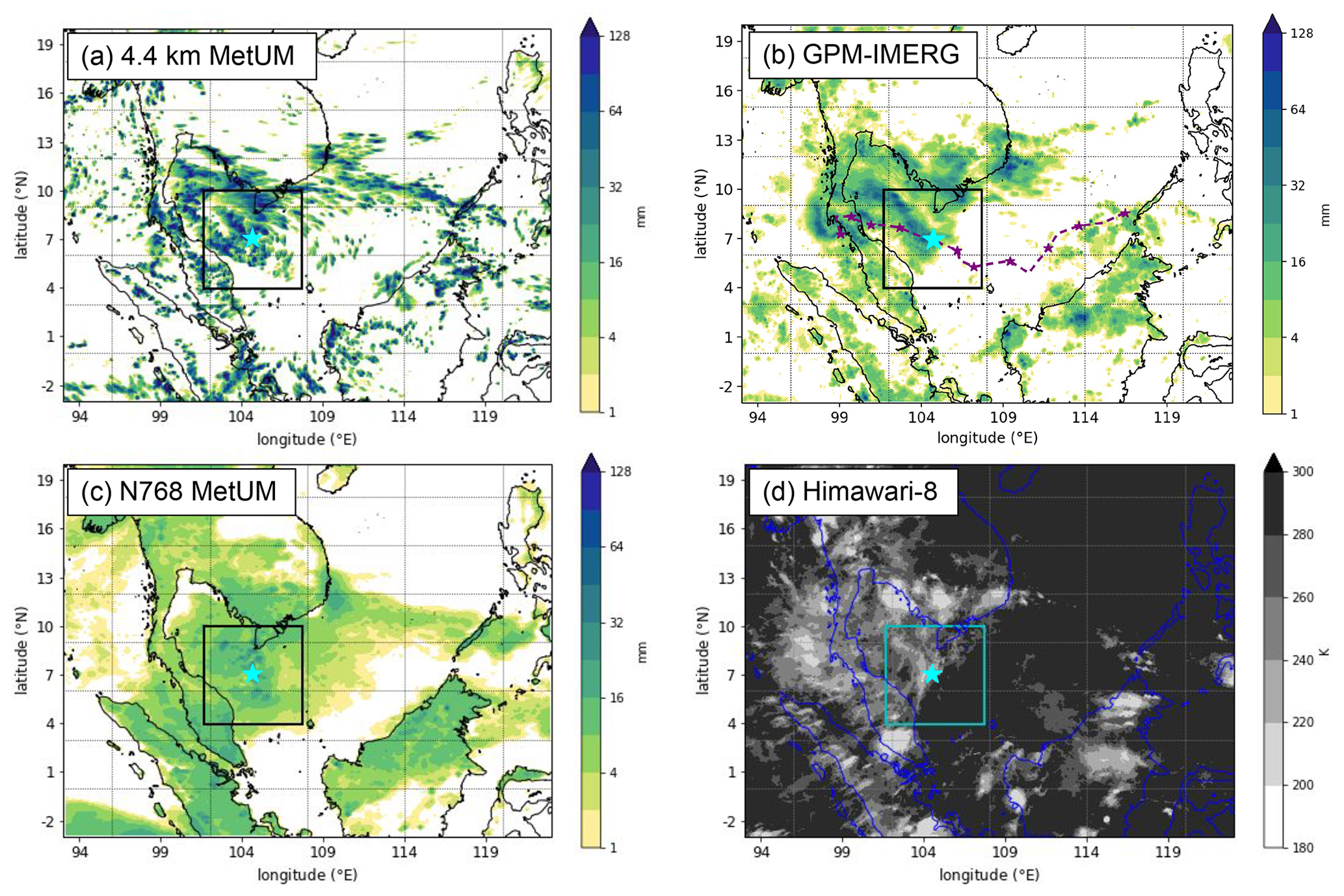
Figure B1The 12 h accumulated precipitation ending at 12:00 UTC on 24 October 2018 (shaded, mm) from (a) 4.4 km MetUM simulation initialised at 12:00 UTC on 21 October 2018, (b) GPM-IMERG satellite product, (c) N768 MetUM simulation initialised at 12:00 UTC on 21 October 2018. (d) Brightness temperature (shaded, K) from the Himawari-8 satellite, valid at 12:00 UTC on 24 October 2018. The cyan star marks the position of the Borneo vortex centre. The dashed purple line in (b) represents the vortex track between 12:00 UTC on 21 October and 12:00 UTC on 26 October 2018, with the smaller purple stars marking the vortex centre position every 12 h.
The source code for the numerical weather prediction (NWP) model used in this study, MetUM (coupled with JULES), is available to use. To apply for a licence to the MetUM, please contact enquiries@metoffice.gov.uk and for permission to use JULES go to https://jules.jchmr.org (Met Office, 2023). The simulations in this study were performed with adapted versions of the Nesting Suite at UM version 11.1 (suite ID u-av356). The SGT tool code sits within the Met Office Science Repository Service (Cullen, 2018). The MIMIC total precipitable water satellite data are made available online by CIMSS at http://tropic.ssec.wisc.edu/real-time/mimic-tpw/indo/main.html (CIMSS, 2023). The GPM-IMERG precipitation satellite data are available at https://disc.gsfc.nasa.gov/datasets/GPM_3IMERGHH_07/summary (Huffman et al., 2019). The ERA5 reanalysis dataset is publicly available to download from the Copernicus Climate Change Service (C3S) Climate Data Store (Hersbach and Coauthors, 2020). Himawari-8 brightness temperature satellite data are publicly available and can be downloaded from the ICARE Data and Services Centre at the University of Lille server after registration (https://www.icare.univ-lille.fr/, AERIS, 2023). The TRACK algorithm is available on the University of Reading's Git repository (GitLab) at https://gitlab.act.reading.ac.uk/track/track (Hodges, 2021). A GitHub repository containing Jupyter notebooks that allow users to reproduce some of the presented figures is available to download at https://doi.org/10.5281/zenodo.10017043 (Hardy et al., 2023).
MC developed the semi-geotriptic balance approximation tool. BH set up and ran the N768 Met Office Unified Model simulation used as input to the balance approximation tool. Project administration and funding acquisition were carried out by JS and JM. SH carried out formal analysis and data visualisation and prepared and wrote the manuscript alongside JM, with contributions from all co-authors. All co-authors helped guide the analysis and reviewed and edited the manuscript.
At least one of the (co-)authors is a member of the editorial board of Weather and Climate Dynamics. The peer-review process was guided by an independent editor, and the authors also have no other competing interests to declare.
Publisher's note: Copernicus Publications remains neutral with regard to jurisdictional claims made in the text, published maps, institutional affiliations, or any other geographical representation in this paper. While Copernicus Publications makes every effort to include appropriate place names, the final responsibility lies with the authors.
The authors would like to thank Stuart Webster (Met Office) for running the suite of nested limited-area Met Office Unified Model forecasts as part of the WCSSP Southeast Asia project. The authors also thank Peter Knippertz and two anonymous reviewers for their constructive comments throughout the review process, which notably improved the manuscript.
This work and three of its contributors (Sam Hardy, John Methven and Juliane Schwendike) were supported by the Met Office Weather and Climate Science for Service Partnership (WCSSP) Southeast Asia project as part of the Newton Fund. The research was also partially funded by the UK Natural Environment Research Council under contract R8/H12/83.
This paper was edited by Peter Knippertz and reviewed by two anonymous referees.
AERIS: ICARE, https://www.icare.univ-lille.fr/ (last access: 12 October 2023), 2023. a
Ahmadi-Givi, F., Craig, G. C., and Plant, R. S.: The dynamics of a midlatitude cyclone with very strong latent heat release, Q. J. Roy. Meteorol. Soc., 130, 295–323, 2004. a
Best, M. J., Pryor, M., Clark, D. B., Rooney, G. G., Essery, R. L. H., Ménard, C. B., Edwards, J. M., Hendry, M. A., Porson, A., Gedney, N., Mercado, L. M., Sitch, S., Blyth, E., Boucher, O., Cox, P. M., Grimmond, C. S. B., and Harding, R. J.: The Joint UK Land Environment Simulator (JULES), model description – Part 1: Energy and water fluxes, Geosci. Model Dev., 4, 677–699, https://doi.org/10.5194/gmd-4-677-2011, 2011. a
Birch, C. E., Webster, S., Peatman, S. C., Parker, D. J., Matthews, A. J., Li, Y., and Hassim, M. E. E.: Scale interactions between the MJO and the western Maritime Continent, J. Climate, 29, 2471–2492, 2016. a
Boettcher, M. and Wernli, H.: A 10-year climatology of diabatic Rossby waves in the Northern Hemisphere, Mon. Weather Rev., 141, 1139–1154, 2013. a, b
Bretherton, F. P.: Baroclinic instability and the short wavelength cut-off in terms of potential vorticity, Q. J. Roy. Meteorol. Soc., 92, 335–345, 1966. a
Bush, M., Allen, T., Bain, C., Boutle, I., Edwards, J., Finnenkoetter, A., Franklin, C., Hanley, K., Lean, H., Lock, A., Manners, J., Mittermaier, M., Morcrette, C., North, R., Petch, J., Short, C., Vosper, S., Walters, D., Webster, S., Weeks, M., Wilkinson, J., Wood, N., and Zerroukat, M.: The first Met Office Unified Model–JULES Regional Atmosphere and Land configuration, RAL1, Geosci. Model Dev., 13, 1999–2029, https://doi.org/10.5194/gmd-13-1999-2020, 2020. a, b
Businger, S.: The synoptic climatology of polar low outbreaks, Tellus A, 37, 419–432, 1985. a
Chambers, C. R. S. and Li, T.: Simulation of formation of a near-equatorial Typhoon Vamei (2001), Meteorol. Atmos. Phys., 98, 67–80, 2007. a
Chang, C.-P. and Wong, T. S.: Rare typhoon development near the Equator, Recent Progress in Atmospheric Sciences: Applications to the Asia-Pacific Region, World Scientific, Singapore, 172–181, https://doi.org/10.1142/9789812818911_0010, 2008. a, b
Chang, C.-P., Erickson, J. E., and Lau, K. M.: Northeasterly cold surges and near-equatorial disturbances over the winter MONEX area during December 1974. Part I: Synoptic aspects, Mon. Weather Rev., 107, 812–829, 1979. a, b
Chang, C.-P., Chen, G. T., Gerish, T. E., and Chou, L. U.: Structure of cyclonic circulations near Borneo during Winter MONEX, Report of the International Conference on the Scientific Results of the Monsoon Experiment, Denpasar, Bali, Indonesia, World Meteorological Organization, Geneva, Section 5, 21–24, 1982. a, b, c, d, e
Chang, C.-P., Liu, C.-H., and Kuo, H.-C.: Typhoon Vamei: an equatorial tropical cyclone formation, Geophys. Res. Lett., 30, 1150, https://doi.org/10.1029/2002GL016365, 2003. a, b
Chang, C.-P., Harr, P. A., and Chen, H.-J.: Synoptic disturbances over the equatorial South China Sea and western Maritime Continent during boreal winter, Mon. Weather Rev., 133, 489–503, 2005a. a, b, c, d, e, f, g
Chang, C.-P., Wang, Z., McBride, J. L., and Liu, C.-H.: Annual cycle of Southeast Asia – Maritime Continent rainfall and the asymmetric monsoon transition, J. Climate, 18, 287–301, 2005b. a
Cheang, B. K.: Synoptic features and structure of some equatorial vortices over the South China Sea in the Malaysian region during the winter monsoon, December 1973, Pure Appl. Geophys, 115, 1303–1333, 1977. a, b, c
Chen, T.-C., Yen, M.-C., Huang, W.-R., and Gallus Jr., W. A.: An East Asian cold surge: Case study, Mon. Weather Rev., 130, 2271–2290, 2002. a, b
Chen, T.-C., Tsay, J.-D., Yen, M.-C., and Matsumoto, J.: The winter rainfall of Malaysia, J. Climate, 26, 936–958, 2013. a, b, c
Chen, T.-C., Tsay, J.-D., Matsumoto, J., and Alpert, J.: Development and formation mechanism of the Southeast Asian winter heavy rainfall events around the South China Sea. Part I: Formation and propagation of cold surge vortex, J. Climate, 28, 1417–1443, 2015a. a, b, c
Chen, T.-C., Tsay, J.-D., Matsumoto, J., and Alpert, J.: Development and formation mechanism of the Southeast Asian winter heavy rainfall events around the South China Sea. Part II: Multiple interactions, J. Climate, 28, 1444–1464, 2015b. a
CIMSS – Cooperative Institute for Meteorological Satellite Services (CIMSS) at the University of Wisconsin-Madison: Morphed Integrated Microwave Imagery Total Precipitable Water (MIMIC-TPW) Satellite Product, http://tropic.ssec.wisc.edu/real-time/mimic-tpw/indo/main.html (last access: 25 September 2023), 2023. a
Clark, D. B., Mercado, L. M., Sitch, S., Jones, C. D., Gedney, N., Best, M. J., Pryor, M., Rooney, G. G., Essery, R. L. H., Blyth, E., Boucher, O., Harding, R. J., Huntingford, C., and Cox, P. M.: The Joint UK Land Environment Simulator (JULES), model description – Part 2: Carbon fluxes and vegetation dynamics, Geosci. Model Dev., 4, 701–722, https://doi.org/10.5194/gmd-4-701-2011, 2011. a
Cullen, M. J. P.: The unified forecast/climate model, Meteorol. Mag., 122, 81–94, 1993. a
Cullen, M. J. P.: The use of semigeostrophic theory to diagnose the behaviour of an atmospheric GCM, Fluids, 3, 72, https://doi.org/10.3390/fluids3040072, 2018. a, b, c, d, e, f
Davis, C. A.: A potential-vorticity diagnosis of the importance of initial structure and condensational heating in observed extratropical cyclogenesis, Mon. Weather Rev., 120, 2409–2428, 1992. a
Dee, D. P. and Coauthors: The ERA-Interim reanalysis – configuration and performance of the data assmilation system, Q. J. Roy. Meteorol. Soc., 137, 553–597, 2011. a
De Vries, H., Methven, J., Frame, T. H. A., and Hoskins, B. J.: Baroclinic waves with parametrized effects of moisture interpreted using Rossby wave components, J. Atmos. Sci., 67, 2766–2784, 2010. a, b, c
Hardy, S., Schultz, D. M., and Vaughan, G.: Early evolution of the 23–26 September 2012 UK floods: Tropical storm Nadine and diabatic heating due to cloud microphysics, Mon. Weather Rev., 145, 543–563, 2017. a
Hardy, S., Methven, J., Schwendike, J., Harvey, B. J., and Cullen, M.: Examining the dynamics of a Borneo vortex using a balance approximation tool, Zenodo [code], https://doi.org/10.5281/zenodo.10017043, 2023. a
Heifetz, E., Bishop, C. H., Hoskins, B. J., and Methven, J.: The counter-propagating Rossby-wave perspective on baroclinic instability. I: Mathematical basis, Q. J. Roy. Meteorol. Soc., 130, 211–231, 2004. a, b, c, d, e, f, g
Hersbach, H. and Coauthors: The ERA5 global reanalysis, Q. J. Roy. Meteorol. Soc., 146, 1999–2049, 2020. a, b
Hodges, K. I.: TRACK tracking and analysis system for weather, climate and ocean data, Gitlab [code], https://gitlab.act.reading.ac.uk/track/track (last access: 13 October 2023), 2021. a
Hoskins, B. J.: The geostrophic momentum approximation and the semi-geostrophic equations, J. Atmos. Sci., 32, 233–242, 1975. a
Hoskins, B. J. and Draghici, I.: The forcing of ageostrophic motion according to the semi-geostrophic equations and in an isentropic coordinate model, J. Atmos. Sci., 34, 1859–1867, 1977. a
Hoskins, B. J. and James, I. N.: Fluid dynamics of the mid-latitude atmosphere, John Wiley & Sons, https://doi.org/10.1002/9781118526002, 2014. a
Hoskins, B. J., McIntyre, M. E., and Robertson, A. W.: On the use and significance of isentropic potential vorticity maps, Q. J. Roy. Meteorol. Soc., 111, 877–946, 1985. a, b
Huffman, G. J., Bolvin, D. T., Braithwaite, D., Hsu, K., Joyce, R., Kidd, C., Nelkin, E. J., Sorooshian, S., Tan, J., and Xie, P.: GPM IMERG Final Precipitation L3 Half Hourly 0.1 degree × 0.1 degree V07 (GPM_3IMERGHH), NASA [data set], https://disc.gsfc.nasa.gov/datasets/GPM_3IMERGHH_07/summary (last access: 12 October 2023), 2019. a, b
Isnoor, K. F. N., Firdianto, P. U., and Rejeki, H. A.: The activity of Borneo vortex as a trigger for extreme rain in West Borneo (case study: 24th–25th January 2017), Earth Environ. Sci., 303, 012061, https://doi.org/10.1088/1755-1315/303/1/012061, 2019. a
Johnson, R. H.: Mesoscale processes, in: The Asian monsoon, Springer, 331–356, https://doi.org/10.1007/3-540-37722-0_8, 2006. a
Johnson, R. H. and Houze, R. A.: Precipitating cloud systems of the Asian monsoon, in: Monsoon meteorology, edited by: Chang, C. P. and Krishnamurti, T. N., Oxford University Press, 298–353, https://ci.nii.ac.jp/naid/10014597164/en/ (last access: 12 October 2023), 1987. a, b
Joos, H. and Wernli, H.: Influence of microphysical processes on the potential vorticity development in a warm conveyor belt: A case-study with the limited-area model COSMO, Q. J. Roy. Meteorol. Soc., 138, 407–418, 2012. a
Juneng, L. and Tangang, F. T.: Long-term trends of winter monsoon synoptic circulations over the maritime continent: 1962–2007, Atmos. Sci. Let., 11, 199–203, 2010. a, b
Juneng, L., Tangang, F. T., and Reason, C. J. C.: Numerical study of an extreme rainfall event during 9–11 December 2004 over the east coast of Peninsular Malaysia, Meteorol. Atmos. Phys., 98, 81–98, 2007. a, b, c, d, e, f
Koseki, S., Koh, T.-Y., and Teo, C.-K.: Borneo vortex and mesoscale convective rainfall, Atmos. Chem. Phys., 14, 4539–4562, https://doi.org/10.5194/acp-14-4539-2014, 2014. a, b, c, d, e, f
Liang, J., Catto, J. L., Hawcroft, M. K., Hodges, K. I., Tan, M. L., and Haywood, J. M.: Climatology of Borneo vortices in the HadGEM3-GC3.1 general circulation model, J. Climate, 34, 3401–3419, 2021. a, b, c, d, e, f, g, h
Liang, J., Catto, J. L., Hawcroft, M. K., Tan, M. L., Hodges, K. I., and Haywood, J. M.: Borneo vortices in a warmer climate, Npj Clim. Atmos. Sci., 6, 1–8, 2023. a
Love, B. S., Matthews, A. J., and Lister, G. M. S.: The diurnal cycle of precipitation over the Maritime Continent in a high-resolution atmospheric model, Q. J. Roy. Meteorol. Soc., 137, 934–947, 2011. a
Manganello, J. V. and Coauthors: Seasonal forecasts of tropical cyclone activity in a hig-atmospheric-resolution coupled prediction system, J. Climate, 29, 1179–1200, 2016. a
Martínez-Alvarado, O., Gray, S. L., and Methven, J.: Diabatic processes and the evolution of two contrasting summer extratropical cyclones, Mon. Weather Rev., 144, 3251–3276, https://doi.org/10.1175/MWR-D-15-0395.1, 2016. a
Met Office: Joint UK Land Environment Simulator (JULES), https://jules.jchmr.org (last access: 12 October 2023), 2023. a
Moore, R. W. and Montgomery, M. T.: Reexamining the dynamics of short-scale, diabatic Rossby waves and their role in midlatitude moist cyclogenesis, J. Atmos. Sci., 61, 754–768, 2004. a, b
Nguyen, D.-Q., Renwick, J., and McGregor, J.: On the presence of tropical vortices over the Southeast Asian Sea-Maritime Continent region, J. Climate, 29, 4793–4800, 2016. a, b
Ooi, S. H., Samah, A. A., and Braesicke, P.: A case study of the Borneo vortex genesis and its interactions with the global circulation, J. Geophys. Res., 116, D21116, https://doi.org/10.1029/2011JD015991, 2011. a, b, c
Ooyama, K.: Numerical simulation of the life cycle of tropical cyclones, J. Atmos. Sci., 26, 3–40, 1969. a
Parker, D. J. and Thorpe, A. J.: Conditional convective heating in a baroclinic atmosphere: A model of convective frontogenesis, J. Atmos. Sci., 52, 1699–1711, 1995. a, b
Paulus, A. W. and Shanas, S. P.: Atmospheric study of the impact of cold surges and Borneo vortex over western Indonesia Maritime Continent area, J. Clim. Weather Forecast., 5, 189, https://doi.org/10.4172/2332-2594.1000189, 2017. a
Priestley, M. D. K., Ackerley, D., Catto, J. L., Hodges, K. I., McDonald, R. E., and Lee, R. W.: An overview of the extratropical storm tracks in CMIP6 historical simulations, J. Climate, 33, 6315–6343, 2020. a
Ramage, C. S.: Monsoon Meteorology, Tech. rep., Elsevier, ISBN 978-0-12-576650-0, 1971. a
Sanchez, C., Methven, J., Gray, S. L., and Cullen, M. J. P.: Linking rapid forecast error growth to diabatic processes, Q. J. Roy. Meteorol. Soc., 146, 3548–3569, https://doi.org/10.1002/qj.3861, 2020. a, b, c
Saragih, R. M. R., Fajarianti, R., and Winarso, P. A.: Atmospheric study of the impact of Borneo vortex and Madden-Julian oscillation over western Indonesian maritime area, J. Phys.: Conf. Ser., 997, 012004, https://doi.org/10.1088/1742-6596/997/1/012004, 2018. a
Steenkamp, S. C., Kilroy, G., and Smith, R. K.: Tropical cyclogenesis at and near the Equator, Q. J. Roy. Meteorol. Soc., 145, 1846–1864, 2019. a
Stoelinga, M. T.: A potential vorticity-based study of the role of diabatic heating and friction in a numerically simulated baroclinic cyclone, Mon. Weather Rev., 124, 849–874, 1996. a
Tangang, F. T., Juneng, L., Salimun, E., Vinayachandran, P. N., Seng, Y.-K., Reason, C. J. C., Behera, S. K., and Yasunari, T.: On the roles of the northeast cold surge, the Borneo vortex, the Madden-Julian Oscillation, and the Indian Ocean Dipole during the extreme 2006/2007 flood in southern Peninsular Malaysia, Geophys. Res. Lett., 35, L14S07, https://doi.org/10.1029/2008GL033429, 2008. a
Trilaksono, N. J., Otsuka, S., and Yoden, S.: A time-lagged ensemble simulation on the modulation of precipitation over west Java in January–February 2007, Mon. Weather Rev., 140, 601–616, 2012. a, b, c, d
Vallis, G. K.: Atmospheric and oceanic fluid dynamics, Cambridge University Press, https://doi.org/10.1017/9781107588417, 2017. a
Walters, D., Boutle, I., Brooks, M., Melvin, T., Stratton, R., Vosper, S., Wells, H., Williams, K., Wood, N., Allen, T., Bushell, A., Copsey, D., Earnshaw, P., Edwards, J., Gross, M., Hardiman, S., Harris, C., Heming, J., Klingaman, N., Levine, R., Manners, J., Martin, G., Milton, S., Mittermaier, M., Morcrette, C., Riddick, T., Roberts, M., Sanchez, C., Selwood, P., Stirling, A., Smith, C., Suri, D., Tennant, W., Vidale, P. L., Wilkinson, J., Willett, M., Woolnough, S., and Xavier, P.: The Met Office Unified Model Global Atmosphere 6.0/6.1 and JULES Global Land 6.0/6.1 configurations, Geosci. Model Dev., 10, 1487–1520, https://doi.org/10.5194/gmd-10-1487-2017, 2017. a
Wangwongchai, A., Sixiong, Z., and Qingcun, Z.: A case study on a strong tropical disturbance and record heavy rainfall in Hat Yai, Thailand during the winter monsoon, Adv. Atmos. Sci., 22, 436–450, 2005. a
Wood, N., Staniforth, A., White, A., Allen, M. R., Diamantakis, M., Gross, M., Melvin, T., Smith, C., Vosper, S. B., Zerroukat, M., and Thuburn, J.: An inherently mass-conserving semi-implicit semi-Lagrangian discretization of the deep-atmosphere global non-hydrostatic equations, Q. J. Roy. Meteorol. Soc., 140, 1505–1520, 2014. a
Wu, M. C. and Chan, J. C. L.: Surface features of winter monsoon surges over South China, Mon. Weather Rev., 123, 662–680, 1995. a
Xavier, P., Lim, S. Y., Abdullah, M. F. A. B., Bala, M., Chenoli, S. N., Handayani, A. S., Marzin, C., Permana, D., Tangang, F. T., Williams, K., and Yik, D. J.: Seasonal dependence of cold surges and their interaction with the Madden-Julian oscillation over Southeast Asia, J. Climate, 33, 2467–2482, 2020. a
Yokoi, S. and Matsumoto, J.: Collaborative effects of cold surge and tropical depression-type disturbance on heavy rainfall in central Vietnam, Mon. Weather Rev., 136, 3275–3287, 2008. a, b
Zappa, G., Shaffrey, L. C., and Hodges, K. I.: Can polar lows be objectively identified and tracked in the ECMWF operational analysis and the ERA-Interim reanalysis?, Mon. Weather Rev., 142, 2596–2608, 2014. a
Aside from the variables discussed in this article, the SGT tool outputs boundary layer height and the time tendencies of θV and the meridional and zonal geostrophic wind components. In addition, two balanced heating tendencies can be output, which use moist (rather than dry) stability from the boundary layer scheme.
- Abstract
- Introduction
- Data and methods
- Case study: 21–26 October 2018
- Vortex structure in the convection-permitting simulation
- The role of balanced flow in Borneo vortex dynamics
- Conclusions
- Appendix A: Deriving the phase speed of diabatic Rossby waves
- Appendix B: Borneo vortex structure during weakening phase
- Code and data availability
- Author contributions
- Competing interests
- Disclaimer
- Acknowledgements
- Financial support
- Review statement
- References