2.1 Study area and campaigns

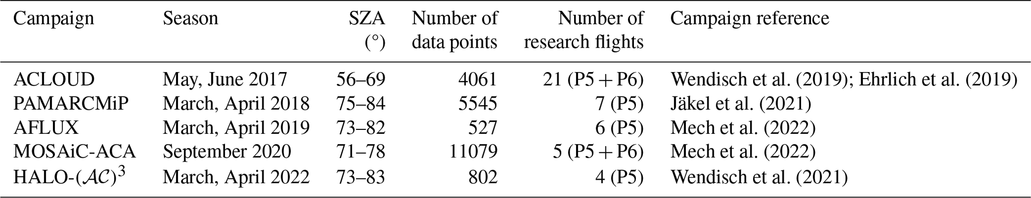
Five flight campaigns were conducted within the collaborative research project “Arctic Amplification: Climate Relevant Atmospheric and Surface Processes, and Feedback Mechanisms” (𝒜𝒞)³ between 2017 and 2022 (Wendisch et al., 2023). The airborne activities were carried out with the research aircraft Polar 5 (P5) and Polar 6 (P6) (Wesche et al., 2016) and focused on observations of Arctic clouds and of the Arctic atmospheric boundary layer as well as surface properties in the European Arctic in different seasons between 2017 and 2022. Table 1 gives an overview of the campaigns considered in this study. Apart from the “Polar Airborne Measurements and Arctic Regional Climate Model Simulation Project” (PAMARCMiP) campaign, which was based at the Danish Villum research station (Station Nord), Greenland (81°36^′ N, 16°40^′ W), all campaigns were based in Longyearbyen (78°13^′ N, 15°38^′ E), Svalbard. The “Arctic CLoud Observations Using airborne measurements during polar Day” (ACLOUD) took place in early summer 2017 and used both P5 and P6. Spring Arctic conditions were observed with P5 only during PAMARCMiP and during the “Airborne measurements of radiative and turbulent FLUXes of energy and momentum in the Arctic boundary layer” (AFLUX) campaign. Within the most recent spring observations in 2022, HALO-(𝒜𝒞)³, both aircraft, P5 and P6, were used with a similar instrumental setup to that during ACLOUD. The set of airborne observations during polar day was completed by the “MOSAiC Airborne observations in the Central Arctic” (MOSAiC-ACA) campaign, which took place in autumn 2020, as an airborne component of the MOSAiC expedition.

Table 1List of campaigns and time frame of observations. Number of used data points is given in total for Polar 5 (P5) and Polar 6 (P6) flights. SZA stands for solar zenith angle.

Download Print Version | Download XLSX

For this study, only low-level (flight altitude below 300 m) flight sections were considered, which were performed above sea ice and open water without clouds between the aircraft and surface. This selection was made to minimize atmospheric masking effects in the albedo observations (Wendisch et al., 2004). Further, the data were filtered with respect to aircraft pitch and roll angles within a range of ±4° to reduce the uncertainties of radiation measurements due to horizontal misalignment (Wendisch et al., 2001). Figure 1 shows the coverage of all selected flight sections for the five aircraft campaigns, together with the sea ice edge as defined from the satellite observation of the sea ice concentration (SIC) derived from the Advanced Microwave Scanning Radiometer 2 (AMSR2) instrument using the method from Spreen et al. (2008). Here, the ice edge is based on 80 % SIC. The strong variations in the sea ice edge position are linked to not only the period of observations but also interannual changes. While the northernmost retreat of sea ice was observed during MOSAiC-ACA in autumn, the southern sea ice edge in the measurement area during ACLOUD in early summer and during the two spring campaigns HALO-(𝒜𝒞)³ and AFLUX does not differ so much. A relatively far northern location of the ice edge for spring conditions was observed during PAMARCMiP in 2018. However, due to the more northern starting point of the aircraft at Station Nord, Greenland, mostly surfaces with more than 80 % of SIC could be overflown. For MOSAiC-ACA, a significant fraction of measurements were carried out in the marginal sea ice zone (MIZ), while for the other campaigns mainly flight sections with SIC larger than 80 % remained after application of the selection criteria. The total numbers of data points and flight days are listed in Table 1. Most flights over sea ice were performed during ACLOUD. However, the largest number of selected measurements was determined for MOSAiC-ACA, where the instrumental setup of the P6 differed from the configuration of the P5, resulting in different time resolutions of the data products.

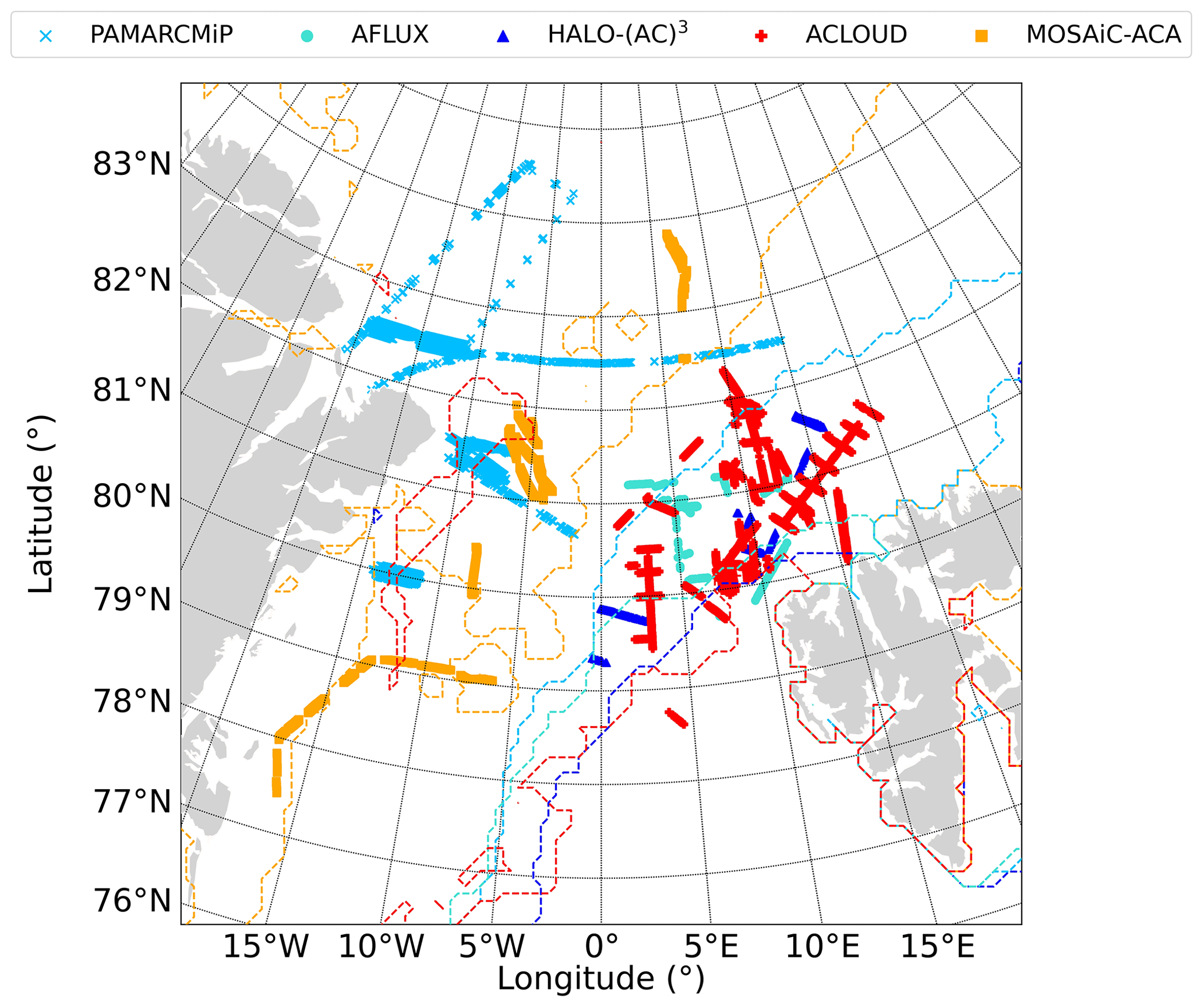
Figure 1Flight sections of surface albedo measurements for all campaigns listed in Table 1. The sea ice edge (based on 80 % SIC) representative of each campaign is plotted with the same color code as the flight track but with dashed lines.

2.2 Instrumentation and products

2.2.2 Camera observations

The classification of surface types is based on images taken by different camera systems. Images were partitioned by manually selected thresholds of the three spectral channels in red, green, and blue (RGB) (Perovich et al., 2002; Jäkel et al., 2019). Depending on the illumination conditions, these thresholds were set using color intensity histograms of training samples.

Digital cameras (Canon EOS 1D Mark III and Nikon D5) with fisheye lenses were used by default during most of the flight experiments on both aircraft. Due to the 180° FOV, such cameras that can be directly related to upward irradiance measurements cover the entire lower hemisphere (Jäkel et al., 2019). The angular resolution is less than 0.1°. Geometric, spectral, and radiometric calibration was applied to characterize the cameras (Ehrlich et al., 2012; Carlsen et al., 2017; Jäkel et al., 2019). For flight tracks which were not observed by a fisheye camera due to instrumental failures, images were extracted from video camera data (miniature camera AXIS P1214-E) with about 1 Hz resolution.

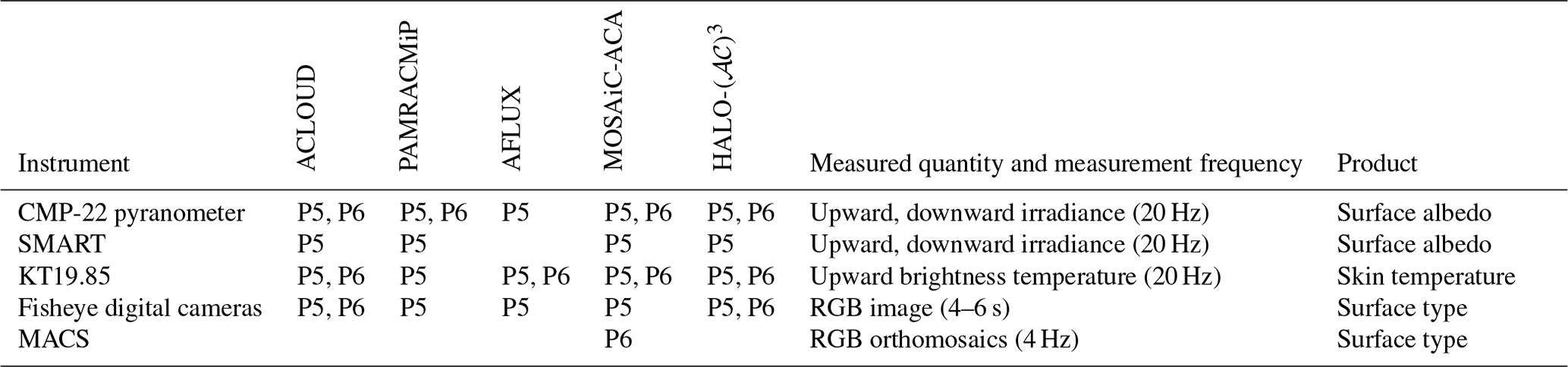
A special version of the scientific Modular Aerial Camera System (MACS) was installed on P6 during MOSAiC-ACA. MACS is equipped with various matrix array cameras that look in the nadir direction and provide images in the visible and near-infrared spectral range. The maximum continuous image acquisition rate is four frames per second, enabling an overlap of images to produce orthomosaics along the flight path. A summary of the relevant airborne instrumentation is given in Table 2.

Table 2Overview of the instrumentation and products of Polar 5 and Polar 6 as used in this study.

Download Print Version | Download XLSX

2.3 Surface albedo parametrization in HIRHAM–NAOSIM

The surface albedo scheme of the coupled regional climate model HIRHAM–NAOSIM was recently revised based on surface broadband albedo measurements performed during the ACLOUD campaign (Jäkel et al., 2019). The original parametrization of the snow albedo, as described in Dorn et al. (2009), was adapted with respect to illumination dependence and snow property changes in terms of threshold temperatures describing the transition between dry and melting snow.

In general, the surface broadband albedo in an inhomogeneous model grid cell is composed of the sum of the surface subtype albedo values weighted by the areal fractions (c) of the respective surface subtypes of open water (subscript ow) and sea ice (subscript i), where sea ice is further divided into snow-covered ice (subscript s), bare ice (subscript bi), and melt ponds (subscript mp):

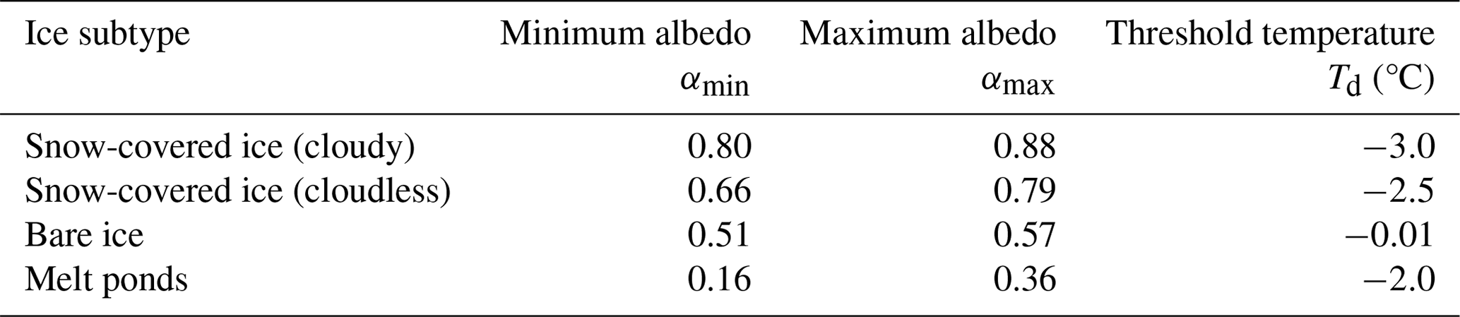
Note that the surface type “white ice”, which is a highly reflective scattering layer on top of melting bare ice (Macfarlane et al., 2023), is not explicitly considered in HIRHAM–NAOSIM. Due to its higher albedo compared to bare ice, white ice is added to the class of snow-covered ice in this work and classified accordingly based on camera observations during the measurement flights. The open-water fraction is not parameterized within this surface albedo scheme and is calculated with a separate prognostic equation. The surface albedo of open water is set to a fixed value of 0.1, while the individual subtype albedo of the ice types is assumed to be variable within a given range of the surface skin temperatures (T_surf) in units of degrees Celsius (Køltzow, 2007; Dorn et al., 2009; Jäkel et al., 2019). A temperature range with temperature thresholds T_d was defined within which the surface albedo varies linearly from maximum (dry ice or snow) to minimum values (melting ice or melting snow). The parameterized surface albedo of the snow-covered ice, for example, is then determined by

with f(T_surf) representing the surface-skin-temperature-dependent function:

The same holds for the two other surface types bare ice and melt ponds. Table 3 summarizes the surface albedo ranges of the individual subtypes and threshold temperatures.

Table 3Minimum and maximum values of the surface albedo for each ice type (snow-covered ice, bare ice, melt ponds) used in the albedo scheme of HIRHAM–NAOSIM.

Download Print Version | Download XLSX

The areal fractions of the sea ice subtypes used in Eq. (4) are estimated by the snow thickness (h_s). For snow-covered sea ice, the fraction is calculated as

where c_s,max is the maximum snow cover fraction of 1.00, and h_0.75=0.03 m giving, the snow thickness at which approximately 75 % of the sea ice is covered by snow (Dorn et al., 2009). The melt pond fraction is subject to the restriction that it is not allowed to exceed the fraction of the sea ice surface not covered with snow (1−c_s). It is parameterized by

with c_mp,max being the maximum melt pond fraction of 0.22 as derived from observational data during SHEBA (Køltzow, 2007; Perovich et al., 2002), which agrees with observations made during MOSAiC (Webster et al., 2022). Locally, however, higher melt pond percentages may occur, e.g., on level first-year ice (Istomina et al., 2015b). Finally, the bare-ice fraction is calculated as the residual ($c_{\mathrm{bi}}=\mathrm{1}-c_{\mathrm{s}}-c_{\mathrm{mp}}$). Note that if the actual ice thickness is lower than 0.25 m, then a linear transition between water and bare-ice albedo is applied to account for the transparent behavior of thin ice (Dorn et al., 2009).

The model output was given with spatial resolution of about 27 km distributed over 200 × 218 grid points on a circum-Arctic domain. For the prognostic variables of the atmospherical model component HIRHAM, a 1 % nudging to reanalysis data of the ERA5 data set (Hersbach et al., 2020) was applied. The HIRHAM–NAOSIM model was run for 2018, covering the time frame of the PAMARCMiP campaign (temporal resolution of 1 h) and for the entire MOSAiC period (temporal resolution of 3 h), including the time frame of the ground-based measurements from spring to autumn 2020 and the period of the aircraft observations during MOSAiC-ACA.

2.4 Methodology for comparison

The outline of the comparison of measured and modeled surface albedo is illustrated in Fig. 2. In the first step the albedo scheme was run offline (i.e., without HIRHAM–NAOSIM), decoupling the two parametrizations of the subtype surface albedo and subtype surface fraction. Because the subtype surface fraction is parameterized as a function of the snow depth, which was not a measured parameter, we used only the parametrization of the subtype surface albedo along with measured values of the prognostic variable T_surf and the measured surface type fractions. The offline evaluation was applied to perform a seasonal comparison between observed and parameterized surface albedo considering data of all aircraft campaigns. In the second step, for an online evaluation, the HIRHAM–NAOSIM output was compared to airborne and ground-based observations. The satellite-based surface albedo derived from Sentinel-3 OLCI was used to characterize the spatial variation on an intermediate grid size scale between local ground-based or aircraft observations and the model output. To match the satellite and model data, all data points of the satellite product that fall into one single grid point of the model were area-averaged accordingly. However, since the satellite product can only be derived for cloudless conditions, the comparison is limited to a few cases.

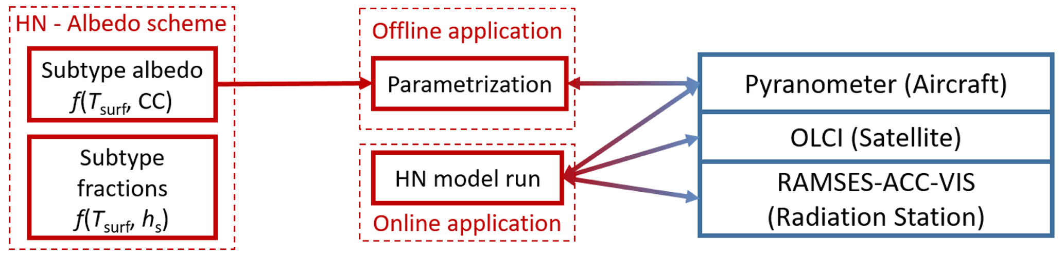
Figure 2Schematics showing the approach for the model-to-measurement comparison. HN stands for HIRHAM–NAOSIM; CC indicates the dependence of the subtype albedo on the cloud coverage.

Download

3.1 Spatiotemporal variability in surface types and surface albedo

An overview of the proportions of classified subtypes along the flight tracks of the five campaigns is shown in Fig. 3 as a stacked area plot. The temporal evolution of the surface broadband albedo and surface skin temperature is given in the corresponding lower panels. Flight sections in spring (Fig. 3a–f) were mostly carried out over snow or white ice (ice with a highly scattering layer on top) with surface skin temperatures below −15 °C. As expected, the variability in the surface albedo depends on the variability in the surface types within the FOV of the downward-looking pyranometer. However, flight sections over snow or white ice also revealed a spatial albedo variability in the range of up to ±0.1 as an effect of surface roughness and variations in snow grain size. In particular for high SZAs, surface roughness tends to reduce the surface albedo compared to a flat surface depending on the feature orientation with respect to the sun (Larue et al., 2020). Note that longer distances were overflown during PAMARCMiP compared to the other two spring campaigns, which explains the strong variation in T_surf (Fig. 3b). The occurrence of open water, caused by either sea ice dynamics or flight sections close to the sea ice edge, leads to a significant increase in surface albedo variability and a decrease in the surface albedo itself down to 0.2. A small percentage of melt ponds was found only in areas with a high fraction of open water (flight on 4 April 2019 during AFLUX) when T_surf is close to 0 °C. The onset of melt pond development on sea ice usually starts in summer, as observed at the end of the ACLOUD campaign (26 June) with melt pond fractions of up to 8 % (Fig. 3g). In general, the surface albedo decreases over time as a consequence of an increase in surface grain size and melt pond fraction, which are both related to the increase in skin temperature during ACLOUD (Fig. 3h). In September the overflown surface showed the most variable conditions (Fig. 3i, j). Surface sections during the first flight were dominated by open water, with surface skin temperatures being in a similar range to that for sea ice (most southern flight track in Fig. 1). Camera images showed that most of the melt ponds were already refrozen and therefore classified as bare ice.

Typically, an increase in sea ice fraction is correlated with an increase in the surface albedo. This relation is influenced by the spectral and directional distribution of the incident solar radiation. Compared to cloudless conditions, clouds may cause an increase in surface broadband albedo due to a spectral shift in the incident radiation. The shift is caused by absorption of solar radiation in the near-infrared spectral range. Figure 3k shows the relationship of the sea ice fraction (white ice plus bare ice) and the surface albedo for all campaigns separated into cloudless and cloudy cases. The surface albedo was averaged within each bin of sea ice fraction (bin size of 10 %). In general, we observed a higher albedo for the same amount of sea ice under cloudy conditions than under cloudless conditions. This effect was more pronounced when a high proportion of sea ice was present. For sea ice fractions around 100 % mean surface albedo, values of 0.76 ± 0.08 (cloudless cases) and 0.81 ± 0.08 (cloudy cases) were calculated. The variability in the surface albedo at 100 % sea ice cover was further examined with respect to a potential dependence on the SZA. For cloudless conditions the correlation coefficient of R=0.37 indicates a low correlation between both quantities. In a cloudy atmosphere the incoming radiation is dominated by the diffuse component, which is independent of the SZA as confirmed by a R value of −0.02. Since the majority of measurements were carried out for surface skin temperatures below −15 °C, melting processes can be ruled out as the cause of the surface albedo variability. Only during the summer campaign (ACLOUD) was a temperature effect on the magnitude of snow albedo observed (Jäkel et al., 2019).

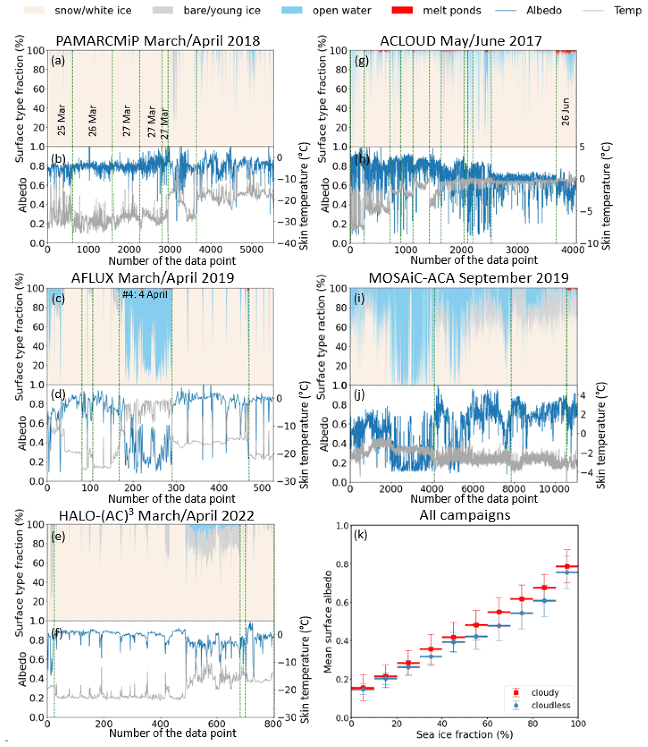
Figure 3(a–j) Temporal changes in surface types, surface albedo (blue lines, left y axis), and surface skin temperature (gray lines, right y axis) for all five flight campaigns. The proportions of surface types are presented as a stacked area plot to identify the predominant subtypes. Vertical green lines separate the individual flight days. Dates given in the panels are explicitly mentioned in the text. (k) Averaged surface albedo as a function of sea ice fraction (bin size of 10 %), separately for cloudless and cloudy conditions. The standard deviation of the averages is represented by thin vertical bars.

Download

3.2 Application of surface albedo scheme (offline evaluation)

The surface albedo scheme of the coupled HIRHAM–NAOSIM model was applied to the measurement data of the different aircraft campaigns to evaluate the performance of the surface albedo parametrization for spring, summer, and autumn conditions. Taking the measured subtype fractions into account, the surface albedo α was parameterized following Eq. (4) using surface-type-specific albedo values defined by Eq. (5). The results separated into cloudy and cloudless cases for spring, summer, and autumn are presented in Fig. 4. The plots show the distributions of the measured and parameterized surface albedo, together with the median value. The parametrization was initially optimized based on the ACLOUD summer campaign data set, leading to reasonable agreement between measurements and parametrization with a root mean square error (RMSE) of 0.05 (Jäkel et al., 2019).

For cloudless conditions, the median values of the measured surface albedo are well represented by the parametrization. A different picture is revealed for cases where clouds are present. While in summer the modeled median surface albedo deviates from the measured value by only 0.01, we observe an overestimation of the modeled median surface albedo of 0.06 in spring. The increase in the surface albedo caused by clouds in summer is much less pronounced in the spring measurements. As this cloud effect depends on the cloud absorption of the downward irradiance in the NIR spectral range, it is assumed that the generally optically thinner clouds in spring do not alter the spectral surface albedo to the same extent as the optically thicker clouds in summer. Therefore, we argue that the cloud parameter in the surface albedo scheme that was defined for summer conditions leads to the overestimation of modeled surface albedo in spring. The distributions shown for autumn (MOSAiC-ACA) are primarily affected by the surface sampled. While measurements under cloudless conditions mostly coincided with flight sections over areas with a high fraction of open water, most of the cloudy cases were sampled over compact ice (see Fig. 3i), which justifies the large difference between the two median values of the cloudless and cloudy distributions. The modes representing the measurements over sea ice indicate a higher parameterized surface albedo than that derived from the measurements. That is possibly caused by the presence of refrozen melt ponds, which were classified as bare ice. Compared to bare ice of considerable thickness that occurs after snowmelt, refrozen melt ponds have little ice thickness on top, resulting in a dark appearance and a lower surface albedo. The model parameters of bare ice may not properly represent such thin ice layers, leading to an overestimation of parameterized surface albedo. In general, however, the distributions were reproduced by the parametrizations for all seasons using the measured sea ice fractions.

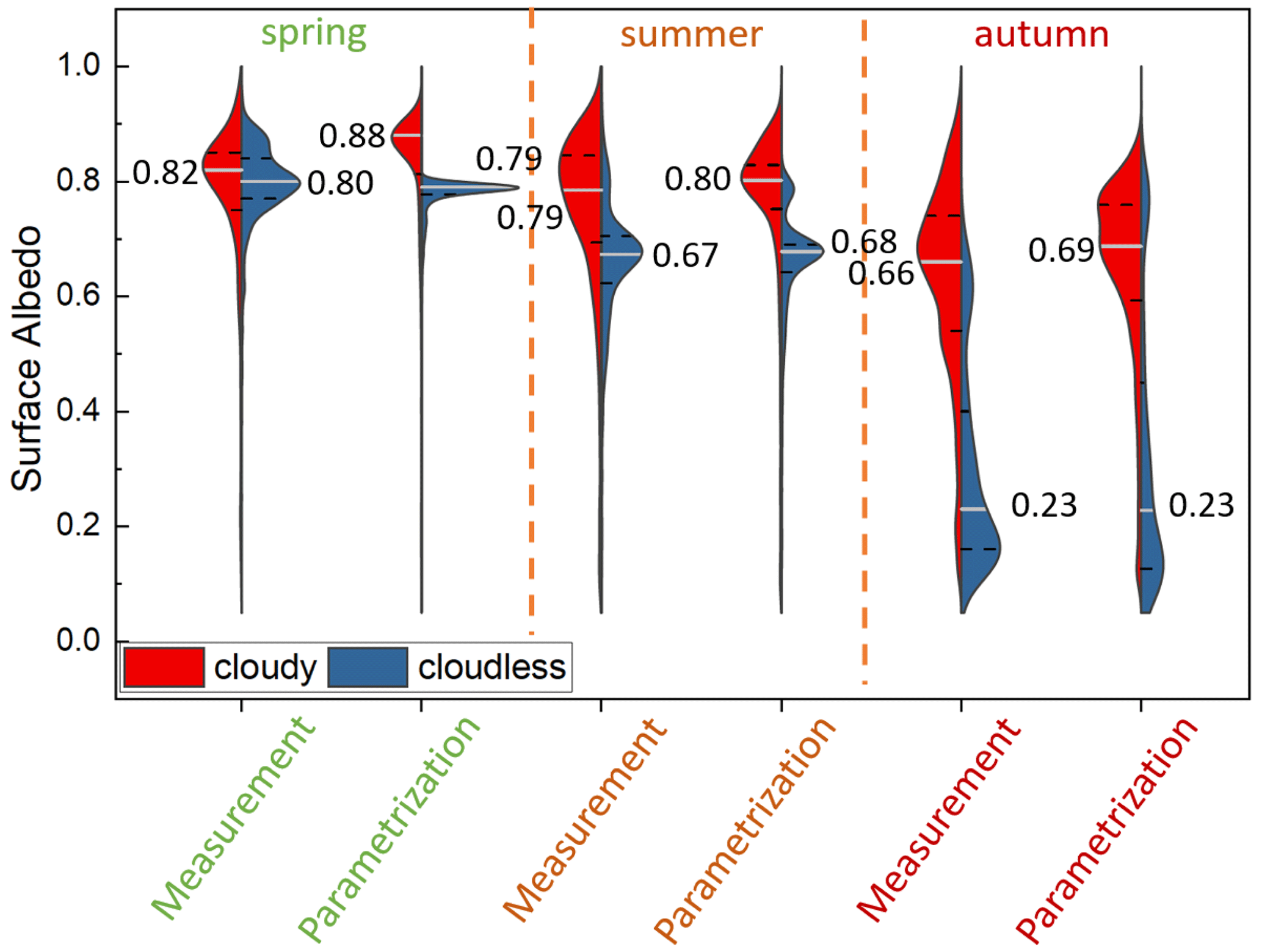
Figure 4Distributions of measured and modeled surface albedo separated into cloudy (red distribution) and cloudless (blue distribution) cases for the seasons spring, summer, and autumn. The median value (also indicated by the white line) is given together with the first and third quartiles (dashed black lines).

Download

3.3 Application of the HIRHAM–NAOSIM model (online evaluation)

3.3.1 Spring case – PAMARCMiP

For spring conditions, HIRHAM–NAOSIM was applied for the time frame of the PAMARCMiP campaign. As an example, the spatial distribution of the modeled surface albedo for the PAMARCMiP area is shown in Fig. 5a. The position of the ice edge can be clearly identified by the sharp gradient of the surface albedo in the lower right corner of this panel. Aircraft-based photos of the surface showed a few refrozen leads along the flight path, but most of the flight sections were carried out over dense drift ice, far away from the MIZ. Despite most of the ocean being completely covered by sea ice, greater variability is observed than in the model results, as shown by the color-coded dots depicting aircraft measurements for each flight day. Small-scale variations arising from surface structure of deformed sea ice, as observed by an airborne laser scanner (Jäkel et al., 2021), cannot be resolved by the model. In contrast, the satellite-based product accounts for variations due to surface roughness (Fig. 5b). A more homogeneous surface albedo was derived for the area north of 82° N latitude. Since surface observations by OLCI are restricted to cloudless scenes, the MPD satellite surface albedo product does not cover the entire area. Therefore, the comparison between satellite-based and modeled surface albedo is limited to the area of data points that is shown in Fig. 5b.

Figure 5c illustrates the distributions of the different surface albedo products. On the left side, the areal comparison of the MPD and HIRHAM–NAOSIM product is shown. As shown in Fig. 5b, we observe greater variability in the higher-resolution satellite data. However, the median values are similar (0.85, 0.86). The smaller second modeled mode (0.77) can be attributed to grid points with a low modeled cloud coverage; hence the snow-covered ice parameter representing cloudless conditions was applied. As the modeled surface albedo depends on cloud cover, the representation of the clouds in the model must be taken into account to evaluate the modeled surface albedo. While the aircraft and satellite observations showed mostly cloudless conditions, the model calculated a cloud cover of about 100 % in most areas. Based on these results, it can be assumed that the match between satellite- and model-derived surface albedo medians results from the compensation of two opposite model biases: the overestimation of modeled cloud coverage, which caused a positive bias in modeled surface albedo, was compensated by a negative bias in modeled cloudless surface albedo. The two distributions of the airborne and the spaceborne surface albedo are shown on the right side of the panel in Fig. 5c. For that, the aircraft measurements were area-averaged with respect to the grid size of the satellite product. The deviation of 0.1 in the median value indicates an overestimation of the satellite product. We applied the spectral-to-broadband conversion of the MPD algorithm (Eq. 3) to the spectral surface albedo measurements of the SMART instrument to rule out larger uncertainties in this conversion, as they might occur under these low-sun conditions during PAMARCMiP. Using the spectral surface albedo of SMART at the six wavelengths together with the spectral weighting coefficients we calculated only a small bias in the broadband measurements with a RMSE of 0.02 and similar mean values of 0.74. Therefore, the spectral-to-broadband conversion can be excluded as a reason for the positive bias of the satellite-based surface albedo.

The temporal variation in the modeled surface albedo is illustrated in Fig. 5d. Each individual line represents the time series of the area-averaged surface albedo for one of the seven overflown areas. In addition, the mean measured surface albedo (including standard deviation) on the corresponding day is shown. Apart from the most southern region overflown on 3 April 2018, no significant change in the surface albedo within the time frame of the campaign was simulated. Short-term variations can be attributed to changes in modeled cloud cover, while larger temporal variations are correlated to the modeled sea ice coverage. The albedo time series of the area overflown on 3 April 2018 shows a pronounced albedo minimum in late March. This is related to a modeled minimum sea ice cover of 86 % for the period shown, which is probably due to ice dynamics. In general, the measured surface albedo shows much greater spatial variability but smaller averaged values than the model. This positive bias of modeled surface albedo cannot be explained by a lower sea ice coverage modeled with HIRHAM–NAOSIM. In fact, the observed sea ice cover averages 99 %, while modeled sea ice cover ranges from 94 % to 99 %. Rather, the biases in the modeled cloud fraction may explain some of the discrepancy between modeled and measured surface albedo. In particular, the first three flights were conducted under cloudless conditions, which would lower the surface albedo from more than 0.85 to 0.76 assuming 95 % sea ice coverage and a snow albedo of 0.79 (Table 3). At least on the following measurement days, the modeled surface albedo is within the standard deviation of the measured surface albedo. However, the area-averaged surface albedo deviates by up to 0.1.

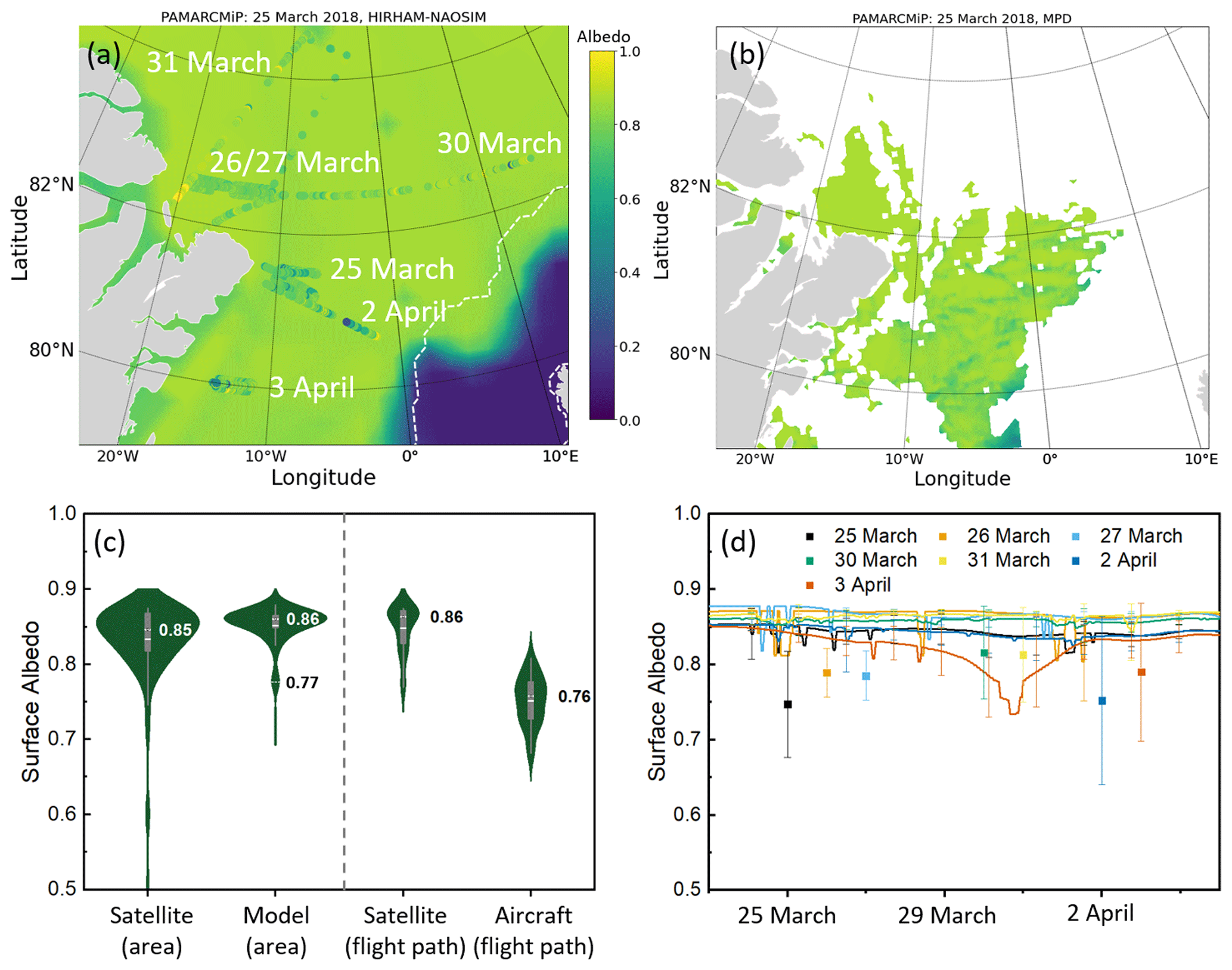
Figure 5(a) Map of the surface albedo as modeled by HIRHAM–NAOSIM for 25 March 2018 (PAMARCMiP). Aircraft observations are plotted as color-coded dots indicating the measured surface albedo for the individual flight days. The dashed white line indicates a SIC of 15 % derived from AMSR observations. (b) Surface albedo under cloudless conditions derived from the OLCI measurements by the MPD retrieval for 25 March 2018 (same color code as in a). (c) Distributions of satellite, model, and aircraft albedo data separately for two regions: the area covered by the satellite data, as shown in (b), and the region along the flight path only. (d) Time series of modeled mean surface albedo for the PAMARCMiP period for the areas covered by the individual flights. The aircraft-measured mean surface albedo (single squares) and standard deviation (vertical bars) are given together.

3.3.2 Autumn case – MOSAiC-ACA

HIRHAM–NAOSIM was further applied for the period of the MOSAiC campaign in 2020. The accompanying aircraft observations in autumn during MOSAiC-ACA revealed 4 d with measurements of the surface albedo, as depicted in Fig. 6a. Other than during PAMARCMiP, the flights were performed over a strongly heterogeneous surface in the MIZ. Again, the modeled sea ice edge can be estimated from the spatial distribution of surface albedo, as the transition to the blue colored areas coincides with the sea ice edge zone. However, AMSR observations of the SIC show a more eastward shift in the sea ice edge compared to the model, as illustrated by the 15 % isoline of SIC in Fig. 6a. This could partly explain the difference between the modeled and measured surface albedo. The modeled albedo map shows a negative bias compared to the measurements along the flight path (overlaying brighter points in Fig. 6a), especially for the flights on 8 and 13 September. The corresponding time series of the area-averaged modeled surface albedo for the four flight regions are shown in Fig. 6b. Compared to the spring data set, a greater spatiotemporal variation is observed which is mainly driven by the variation in surface type distribution. Since HIRHAM–NAOSIM mostly simulated a cloud coverage of 100 %, the variability in the surface albedo cannot be attributed to the use of different parametrizations for cloudy and cloudless conditions.

The measured area-averaged surface albedo shows the best agreement for the region overflown on 2 September, although the surface albedo along the northernmost section of this flight path was partly overestimated by the model. During the flight carried out on 7 September 2020, the area-averaged surface albedo is slightly underestimated by the model but is still within the range of standard deviation of the measurements. This differs from the results of the two last flights, which show a significant negative bias of the modeled surface albedo. Both measurements and the model revealed a similar cloud coverage. This suggests that especially the parametrization of the surface types affects the representation of the modeled surface albedo.

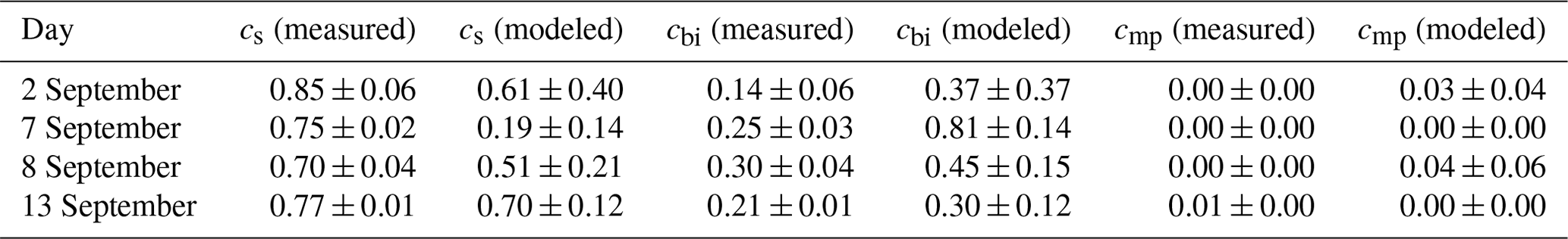
Since the model assumes a sea ice edge closer to the areas observed by the aircraft, the modeled fraction of open water is significantly higher than the measurements show. To exclude the open-water fractions, we only considered the three sea ice subtypes and scaled them such that they sum up to a fraction of one. This makes them more comparable to the modeled sea ice fractions c_mp, c_s, and c_bi (Eq. 6). We further reduced the data sets, where c_ow exceeds 0.8. Table 4 summarizes the area-averaged surface type fractions as derived from the model and the aircraft observations. Melt ponds affect neither the modeled nor measured fractions. The relationship between snow depth and c_s (Eq. 7) leads to an underrepresentation of snow-covered ice for all days because of either insufficient modeled snow depth or the relationship itself. Unfortunately, snow depth observations are not available to look into the cause of the differences. However, the spread of the modeled fractions is significantly larger than those derived from camera observations due to the more heterogeneous surface conditions at the modeled sea ice edge.

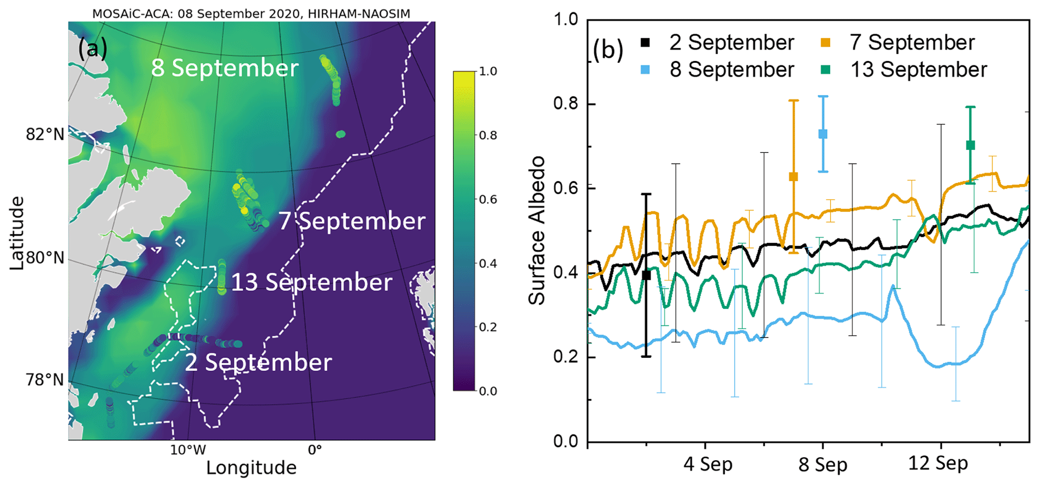
Figure 6(a) Map of the surface albedo as modeled by HIRHAM–NAOSIM for 8 September 2020 (MOSAiC-ACA). Aircraft observations are plotted as color-coded dots indicating the measured surface albedo for the individual flight days. The dashed white line indicates a SIC of 15 % derived from AMSR observations. (b) Time series of modeled mean daily surface albedo for the MOSAiC-ACA period for the areas covered by the individual flights. The standard deviation of the area average is represented by thin vertical bars. The measured mean surface albedo and standard deviation are shown, similar to in Fig. 5d.

Table 4Area-averaged surface type fractions of snow-covered ice (c_s), bare ice (c_bi), melt ponds (c_mp), and open water (c_ow) derived from the camera classification and modeled by HIRHAM–NAOSIM. The standard deviation demonstrates the spatial variation.

Download Print Version | Download XLSX

3.3.3 Polar-day time series – MOSAiC

During MOSAiC, the seasonal evolution of the surface albedo was measured by autonomous radiometers. In this study, data from one of the RAMSES stations (2020R12, following the notation of Tao et al., 2024) were used; 2020R12 was deployed on second-year ice at site L3 of the MOSAiC distributed network (Nicolaus et al., 2022). This data set provides almost-continuous time series of irradiance measurements between 24 April and 7 August 2020, which allow the transition from dry to wet snow to be observed. We applied the two corrections according to Eqs. (1) and (2) to the ground-based observation of the autonomous radiometers. The time series of original and corrected measured surface albedo (April to August) are shown in Fig. 7a. As the radiometer data were not filtered with respect to the atmospheric conditions, we assume that the two time series, representing either cloudless or cloudy conditions, indicate the range of the surface broadband albedo. The plot shows several characteristics of the melting season, as discussed in Tao et al. (2024). Prior to 26 May, the surface was covered with dry snow, resulting in the highest surface albedo. With the onset of melting, an initial melt pond formed directly under the radiation sensor so that a first minimum of surface albedo was observed on 29 May. The snowfall caused the surface albedo to increase thereafter, but not to the earlier level, as wet-snow conditions prevailed instead. A second major melt pond event was observed with a minimum surface albedo on 25 June. The later increase in surface albedo is related to melt pond drainage. After that, the surface was dominated by the surface scattering layer (SSL).

Satellite-based surface albedo data were available for 5 cloudless days during the period of ground-based observations. The data were averaged over the area corresponding to the extent of the HIRHAM–NAOSIM grid pixel covering the radiometer site. For 5 and 6 June, when the melt pond was covered by new snow, the satellite-based surface albedo exceeds the ground-based values (Fig. 7a). On 21 and 22 June, satellite- and ground-based measurements showed a similar mean surface albedo of 0.69. For the observed cloudless conditions, Eq. (1) can be applied to correct the radiometer measurements. The largest differences were found after the drainage of the observed melt pond on 30 June. Here, the radiometer measurement exceeds the satellite-based surface albedo product by more than 0.1. One can assume that the local observation was not representative of the larger area observed by the satellite, which captured a higher fraction of melt ponds with a lower surface albedo.

The time series of the modeled surface albedo by HIRHAM–NAOSIM has three major phases. The first ends with the onset of melting similar to the ground-based measurements, on 26 May. While the radiometer measurements showed a decrease in surface albedo due to a first melt pond event, the modeled albedo only decreased due to the transition to wet snow. Melt ponds were not modeled at this stage, as can be seen in Fig. 7b. In fact, snow-covered ice was the dominant surface type fraction. A significant change in surface type fractions was also modeled for 28 June 2020 3 d after the observed formation of the second melt pond. Within 2 d pond formation started simultaneously with the transformation of snow-covered ice to bare ice due to snowmelt. The timing of the second melt pond formation was well simulated by the model. After the formation of melt ponds, however, the modeled surface albedo was significantly underestimated compared to the observations by the satellite and the ground-based RAMSES station. The modeled surface albedo remains at a low level (α≈0.4) after 28 June, while the measured surface albedo (α>0.6) increases again due to surface drainage. The MPD OLCI satellite retrieval also determines the melt pond fraction, which was about 25 % on 30 June (Niehaus et al., 2023) and thus higher than the modeled melt pond fraction (20 %). We also assume that the predominantly modeled bare-ice fraction, with its low surface albedo, contributes to the albedo model bias. In the field, however, the surface albedo of the melting ice remained relatively high due to the presence of a brighter SSL, which is not taken into account in HIRHAM–NAOSIM.

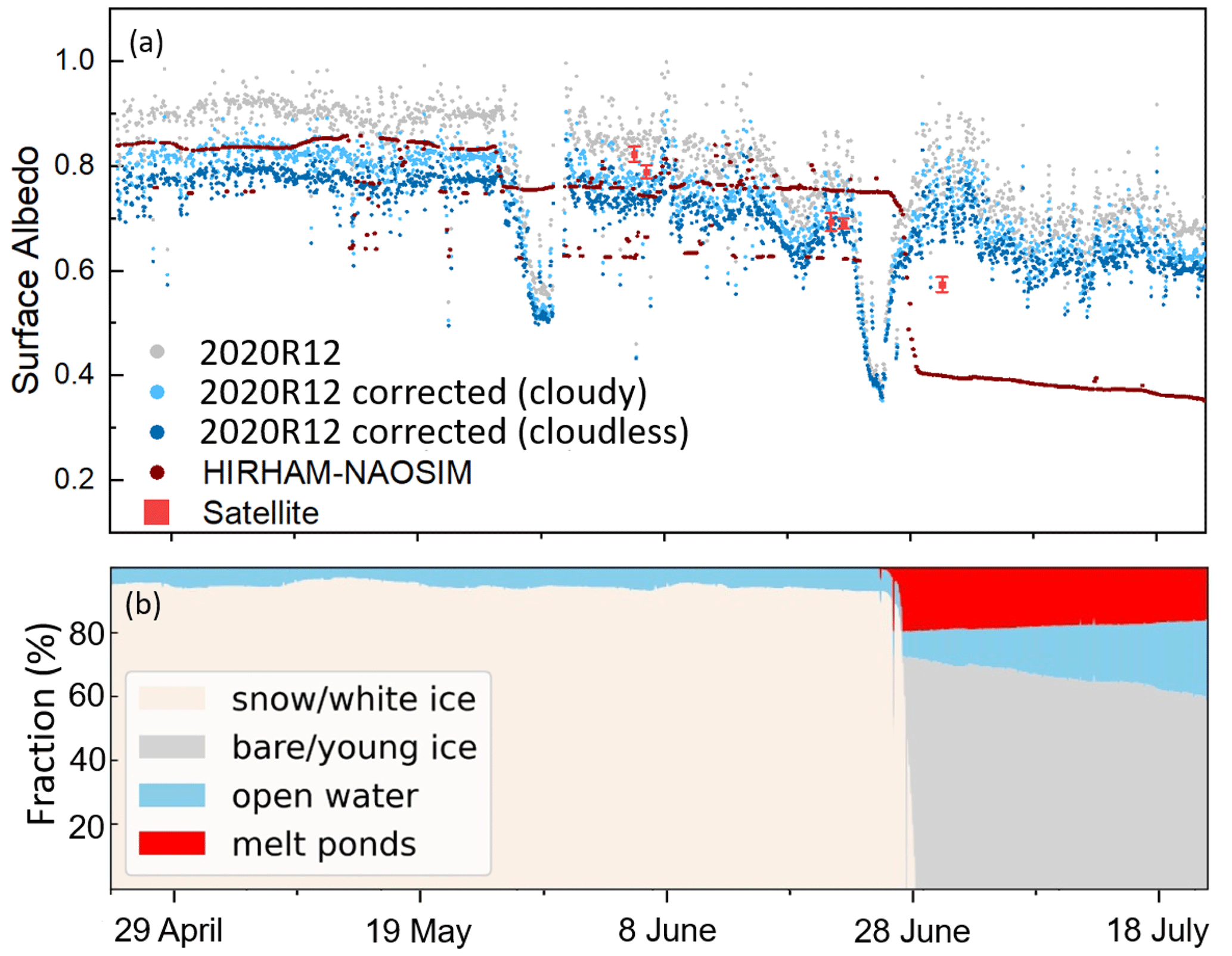
Figure 7(a) Time series of surface broadband albedo (original and corrected) derived from radiometer measurements and HIRHAM–NAOSIM modeling during MOSAiC 2020. Short-term variations in modeled surface albedo are attributed mainly to changes in cloud cover. Area-averaged satellite-based OLCI MPD retrieval results covering the area of the model grid cell are shown for 5 cloudless days (red symbols). (b) Temporal evolution of surface type fractions calculated by HIRHAM–NAOSIM.

Download

4.1 HIRHAM–NAOSIM model results

The net solar irradiance at the surface is defined as the difference between downward and upward irradiance:

The difference between the modeled and measured net irradiances is calculated to estimate the impact of the model bias for the solar radiative energy budget:

Based on the model results introduced in Sect. 3.3, we compared the measured and modeled net irradiance for all model grid points that covered the selected flight tracks during the PAMARCMiP and MOSAiC-ACA campaign. Figure 8 shows the scatterplot of both net irradiances. The corresponding standard deviation illustrates the variability in F_net with a maximum of about 60 W m⁻². The correlation R between the measured and modeled net irradiances is 0.80, and the RMSE of the model is 30.2 W m⁻², with deviations increasing accordingly for larger differences between measured and modeled surface albedo.

Not only do the F_net differences between measurements and the model depend on Δα, but we must also take into account the difference in the downward irradiance (ΔF^↓). A negative ΔF^↓ (smaller symbols in Fig. 8) may occur when the modeled extinction of F^↓ caused by modeled clouds is higher than an observation would show. This is especially the case when cloudless situations were observed but not modeled. It would lead to an underestimation of the modeled net irradiance, assuming the same surface albedo. In fact, a mean negative bias of the modeled F^↓ (mean $\mathrm{\Delta }{F}^{\downarrow }=-\mathrm{31}$ W m⁻²) was found, which can be related to an overestimation of the modeled cloud cover. However, the downward irradiance itself also depends on the surface albedo. In particular, F^↓ under cloudy conditions is enhanced for brighter surfaces due to multiple-scattering between the surface and cloud base. A positive surface albedo bias would lead to a positive bias in F^↓, assuming a similar cloud representation. On average Δ α was 0, indicating a small effect of surface albedo on the modeled F^↓.

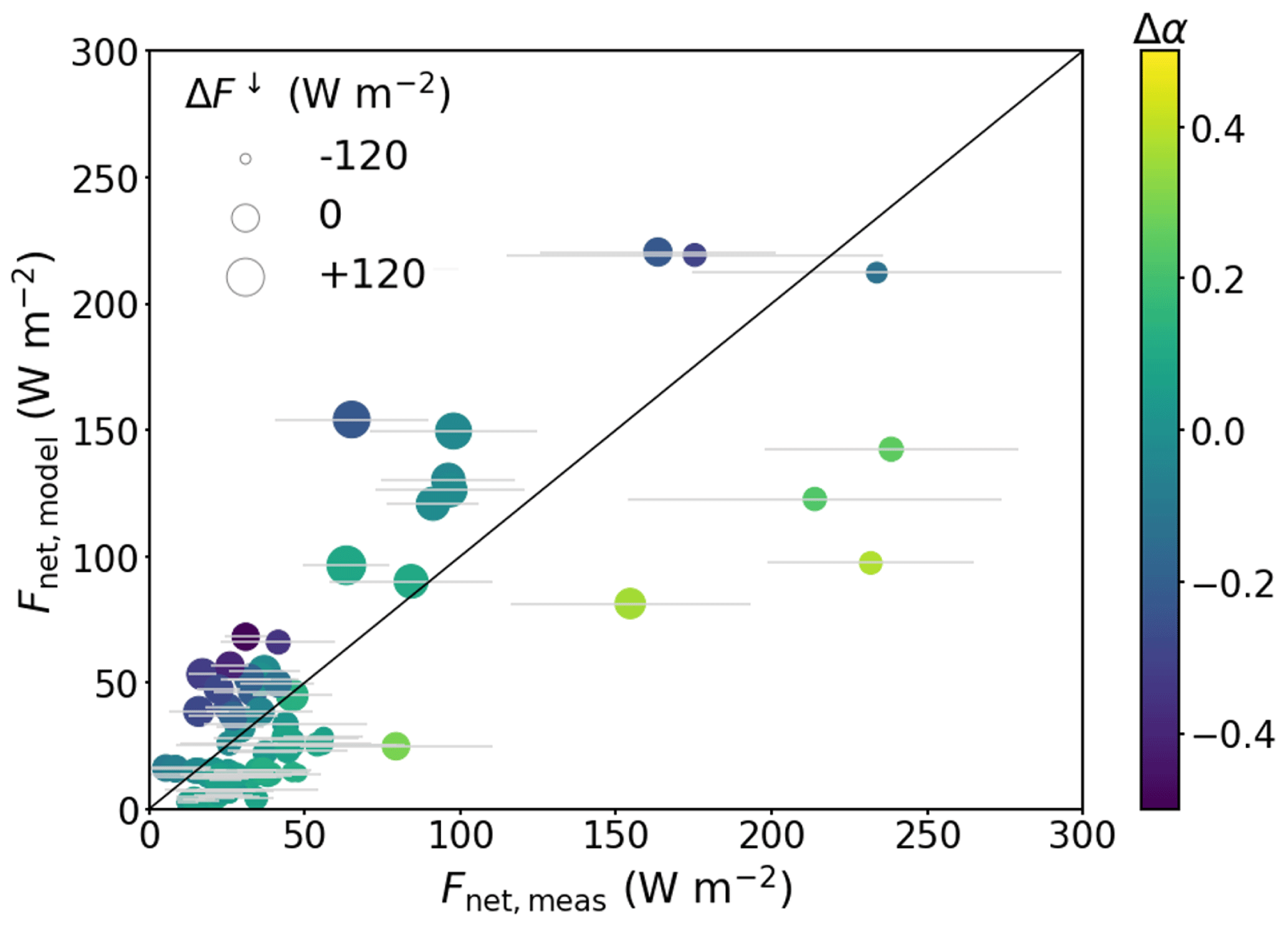
Figure 8Scatterplot of net irradiance based on measured and modeled surface albedo covering the flights performed during PAMARCMiP and MOSAiC-ACA. The horizontal bars indicate the standard deviation of the averaged measured F_net. Color code gives the surface albedo difference ($\mathrm{\Delta }\mathit{\alpha }={\mathit{\alpha }}_{\mathrm{model}}-{\mathit{\alpha }}_{\mathrm{meas}}$) and the symbol size the difference between the modeled and measured downward irradiance.

Download

Overall, both cloud properties and surface albedo must be well represented for modeling net irradiance correctly. To estimate whether the representation of clouds or the surface albedo potentially contributes more to the uncertainty in F_net, we calculated the standardized regression coefficients. Such standardization is useful as the parameters are expressed in different units. HIRHAM–NAOSIM provides the total cloud water path (CWP) as a measure of the cloud microphysics. To account for the available incident radiation we also consider the SZA as a third parameter. The standardized regression coefficients β_j with j being either α, CWP, or SZA are calculated directly from the unstandardized regression coefficient b_j between F_net and the variables and the standard deviations (σ) of the variables:

This means that a change of 1 standard deviation in one of the parameters is associated with a change of β standard deviations in F_net so that the more important variable will have the maximum absolute value of β_j. For the analyzed cases during MOSAiC-ACA and PAMARCMiP we found the strongest impact of the surface albedo (${\mathit{\beta }}_{\mathit{\alpha }}=-\mathrm{0.80}$) and less impact of the CWP (${\mathit{\beta }}_{\mathrm{CWP}}=-\mathrm{0.38}$) and SZA (${\mathit{\beta }}_{\mathrm{SZA}}=-\mathrm{0.23}$). This highlights the importance of a reliable surface albedo parametrization for modeling a realistic surface energy balance. However, we expect a seasonal dependence of the standardized regression coefficients. According to Eq. (11), a stronger variability in the individual parameters contributes to a higher magnitude of β_j. In summer, for example, clouds tend to have a higher cloud water path with greater variability, while the surface albedo reaches its minimum. Therefore, it is assumed that the contribution of the surface albedo bias to the F_net uncertainty is reduced, while the model representation of cloud properties becomes more important compared to the two periods shown in this study.

4.2 Offline evaluation results

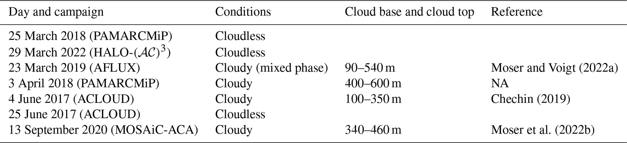
In contrast to the study of the HIRHAM–NAOSIM results, the application of the offline evaluation allows dependencies of the F_net bias to be considered for the comparison of the parametrization with the airborne measurements. The measured subtype fractions were used to identify only the influence of the bias of the parameterized surface albedo on F_net without having to consider the uncertainties in the subtype fraction parametrization. The net irradiance was determined along the flight path for 7 selected days during all five flight campaigns, covering cloudy and cloudless conditions. Radiative transfer simulations (Appendix A) were performed for these cases using the measured and parameterized surface albedo. In this way, the sensitivity of net irradiance to surface albedo was quantified under the same predefined atmospheric conditions. These conditions matched the measurements made during the selected flights (see Appendix A). For cloudless conditions broadband upward and downward irradiances were simulated so that the direct impact of surface albedo can be derived from the difference in the resulting net irradiance, according to Eq. (10). For cloudy conditions the setup of the radiative transfer model required information of the cloud microphysical properties. We estimated these profiles along the flight path as follows: where appropriate, we used profile in situ measurements of the liquid or ice water content and particle size to define a standard cloud profile. In a second step this standard profile was adjusted by scaling the water content of the profile so that the measured and the simulated downward irradiances matched at each measurement point along the flight track. This provides an estimate of the cloud optical depth (COD). Radiative transfer simulations were then performed using this scaled cloud profile and the parameterized surface albedo to derive F_net,model. A table summarizing the corresponding microphysical profiles can be found in Appendix A.

Figure 9a shows a scatterplot of the net irradiances that were derived from the measured and parameterized surface albedo. A significantly smaller spread between measured and parameterized F_net with R=0.97 and RMSE = 13.5 W m⁻² is obtained. We identify two clusters. The first one represents all spring and autumn cases and data derived for cloudy conditions in summer (F_net<100 W m⁻²). As an effect of a low downward irradiance and a high surface albedo, the lowest F_net values were derived for spring cases under cloudy conditions that are dominated by a high fraction of dry snow surfaces. The second cluster (F_net: 150–350 W m⁻²) indicates the cloudless cases in summer that are obtained at a lower SZA (56–66°) and low surface albedo due to wet snow. Figure 9b illustrates the dependence of ΔF_net on Δα and SZA. The linear relationship between ΔF_net and Δα for similar atmospheric conditions results directly from the correlation of surface albedo and upward irradiance. A positive bias of the parameterized surface albedo leads to a higher upward irradiance and consequently results in a lower F_net compared to the measurements. The maximum impact of the albedo bias on ΔF_net is derived for cloudless summer conditions ($\mathrm{\Delta }{F}_{\mathrm{net}}=\pm \mathrm{80}$ W m⁻²). For the same range of Δα in spring, ΔF_net is found to be less than half of its magnitude in summer ($\mathrm{\Delta }{F}_{\mathrm{net}}=\pm \mathrm{35}$ W m⁻²). This means that the bias of modeled surface albedo can have greater effects on the simulated net solar irradiance at the surface in summer compared to spring. In spring, however, we observed from the flight measurements an increased albedo bias with a wider distribution ($\mathrm{\Delta }\mathit{\alpha }=\mathrm{0.02}\pm \mathrm{0.07}$) than in summer ($\mathrm{\Delta }\mathit{\alpha }=\mathrm{0.00}\pm \mathrm{0.04}$). The deviation from the linear relationship between ΔF_net and Δα at a similar SZA can be attributed to different cloud conditions. We used the estimated cloud optical depth to illustrate the cloud impact on ΔF_net. Figure 9c shows the frequency distribution of ΔF_net of all analyzed cases separated into three cloud classes. Accordingly, the cloudless cases comprise the largest range of values with a low mean positive bias (median: 2.5 W m⁻²). The F_net bias for cases with optically thicker clouds (COD >5) is distributed around its median value of 0.1 W m⁻², showing the narrowest distribution (interquartile range: 10.4 W m⁻²). A clear negative F_net bias (median: −6.4 W m⁻²) is observed for optically thin clouds (COD <5), which results from the systematic overestimation of the cloud enhancement effect for α_model in the case of optically thin clouds. A better description of the surface albedo dependence on the cloud property is required to overcome this systematic effect.

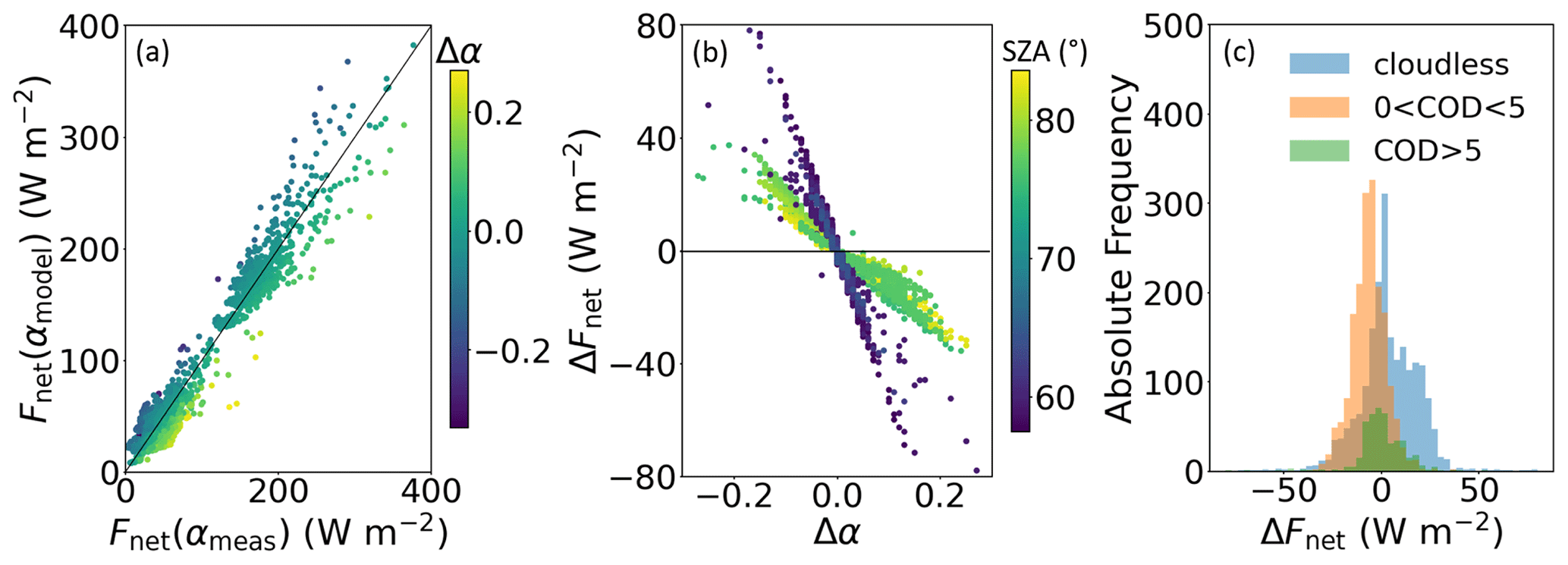
Figure 9(a) Scatterplot of net irradiance based on measured and parameterized surface albedo covering flights performed in spring, summer, and autumn. The color code gives the surface albedo difference ($\mathrm{\Delta }\mathit{\alpha }={\mathit{\alpha }}_{\mathrm{model}}-{\mathit{\alpha }}_{\mathrm{meas}}$). (b) Difference between net irradiance with parameterized surface albedo and net irradiance with measured surface albedo as a function of surface albedo difference. Colors indicate the solar zenith angle. (c) Frequency distribution of ΔF_net separated into three cloud classes: cloudless, thin clouds with cloud optical depth (COD) lower than 5, and clouds with COD larger than 5.

Download