the Creative Commons Attribution 4.0 License.
the Creative Commons Attribution 4.0 License.
 | 15 Dec 2023
A random forest approach to quality-checking automatic snow-depth sensor measurements
Giulia Blandini
Francesco Avanzi
Simone Gabellani
Denise Ponziani
Hervé Stevenin
Sara Ratto
Luca Ferraris
Alberto Viglione
State-of-the-art snow sensing technologies currently provide an unprecedented amount of data from both remote sensing and ground sensors, but their assimilation into dynamic models is bounded to data quality, which is often low – especially in mountain, high-elevation, and unattended regions where snow is the predominant land-cover feature. To maximize the value of snow-depth measurements, we developed a random forest classifier to automatize the quality assurance and quality control (QA/QC) procedure of near-surface snow-depth measurements collected through ultrasonic sensors, with particular reference to the differentiation of snow cover from grass or bare-ground data and to the detection of random errors (e.g., spikes). The model was trained and validated using a split-sample approach of an already manually classified dataset of 18 years of data from 43 sensors in Aosta Valley (northwestern Italian Alps) and then further validated using 3 years of data from 27 stations across the rest of Italy (with no further training or tuning). The F1 score was used as scoring metric, it being the most suited to describe the performances of a model in the case of a multiclass imbalanced classification problem. The model proved to be both robust and reliable in the classification of snow cover vs. grass/bare ground in Aosta Valley (F1 values above 90 %) yet less reliable in rare random-error detection, mostly due to the dataset imbalance (samples distribution: 46.46 % snow, 49.21 % grass/bare ground, 4.34 % error). No clear correlation with snow-season climatology was found in the training dataset, which further suggests the robustness of our approach. The application across the rest of Italy yielded F1 scores on the order of 90 % for snow and grass/bare ground, thus confirming results from the testing region and corroborating model robustness and reliability, with again a less skillful classification of random errors (values below 5 %). This machine learning algorithm of data quality assessment will provide more reliable snow data, enhancing their use in snow models.
- Article
(6276 KB) - Full-text XML
- BibTeX
- EndNote


Snow plays a key role in shaping the dynamics of the hydrological cycle, influencing streamflow as well as surface and groundwater storage availability in terms of quantity, quality, and timing (Dettinger, 2014). Snow-depth measurements and related snow water equivalent (SWE) data provide insightful knowledge, exploitable for water management, hydrological forecasting, and emergency preparedness (Hartman et al., 1995). Recent analyses prove that a significant reduction in streamflow is often a direct consequence of a reduction in precipitation as snow, exacerbated by temperature increase (Berghuijs et al., 2014). In this framework, snow droughts severely affect the hydrological cycle (Harpold et al., 2017), leading to hydrological droughts (Toreti et al., 2022). Additionally, the snow cover and ice cover are key climate change indicators, especially because the high albedo and low thermal conductivity of snow cover strongly affect the global radiant energy balance and the atmospheric circulation (Flanner et al., 2011). A decline in snowfall and snow cover on the ground not only affects water supplies, but also alters the equilibrium of wildlife and vegetation as well as transportation, cultural practices, travel, and recreation for millions of people (Bair et al., 2018).
Assessing the implication of snow-driven hydrological processes on streamflow and precipitation events helps with resource management. Indeed, a more in-depth understanding of snowmelt implications for the time and quantity of freshet supports forecasting for water management, dealing with water security and water-related vulnerability. Most importantly, better understanding of snow processes enables the development of a sustainable water resource carrying capacity, which is crucial to cope with the shift in water balance caused by climate change (Maurer et al., 2021). In this framework, physics models are often used to support engineers, scientists, and decision-makers in real world hydrological operations.
Contemporary environmental technologies have made it possible to easily gain new information, even in real time, with an increasing quantity of data made available from remote sensing and more sophisticated ground sensors. However, high-resolution data of snow come with a variety of noise sources that make quality assurance and quality control (QA/QC) indispensable to use such data in snowpack modeling (Avanzi et al., 2014; Bavay and Egger, 2014). A recurring case in this context is snow-depth data, with two frequent noise categories: (1) snow vs. grass ambiguity due to snow-depth ultrasonic sensors detecting not only snow cover but also plant and grass growth in spring and summer (Vitasse et al., 2017) and (2) random errors (e.g., spikes, anomalous data points that protrude above or below an interpolated surface).
Traditionally, in the field of snow cover and snow-depth monitoring, QA/QC procedures have been carried out by visual inspection, heavily depending on subjective expert knowledge (Robinson, 1989). While expert-knowledge QA/QC is arguably the most reliable approach to data processing, these practices are not easily reproducible or transferable and are highly time-consuming (Fiebrich et al., 2010). In this context, QA/QC with regard to grass detection is often based on static climatological or minimum-snow-depth thresholds, while random errors are generally detected based on maximum-snow-depth thresholds or criteria based on signal variance (Avanzi et al., 2014). An exception in this regard is the approach implemented by the Swiss MeteoIO algorithm for grass detection, which however requires information on surface snow temperature, ground surface temperature, and radiation (Bavay and Egger, 2014).
In view of this knowledge gap, Jones et al. (2018) highlight the burden of subjectivity that may affect overall data quality and comparability, stressing how even expert scientists are not immune to mistakes, especially if performing recurrent unguided quality-checking procedures. As explained by Schmidt et al. (2018), automatic environment data quality control literature is still fragmented, with heterogeneous applications. It is clear then the necessity for a quality-checking procedure that ought to be defined through common and iterable guidelines to guarantee repeatability and consistency (Jones et al., 2018).
Considering the ever-growing volume of data and the limitations arising from traditional QA/QC procedures, here we follow intuitions from Schmidt et al. (2018) and propose the use of machine learning to automatically quality check high-resolution snow-depth sensor data from ultrasonic sensors. The choice of machine learning was driven by its efficiency in dealing with big datasets and as a valid reinforcement of traditional analytic tools (Ferreira et al., 2019). Moreover, machine learning techniques may also be able to handle different data formats more easily that traditional statistical tools, while they deal better with a combination of features that are a priori unknown to the developer (Zhong et al., 2021).
We trained and validated our algorithm using as the training dataset an already classified pool of 18 years of hourly data from 43 snow-depth sensors in Aosta Valley. We then expanded the validation by applying the final algorithm over 3 years of independent data from 27 stations across the rest of Italy (no further tuning in this case) as a pilot case study to assess the applicability of this algorithm to larger and more heterogeneous domains. This research thus answered three questions. (i) What is the accuracy of a random forest classifier algorithm in automatically performing QA/QC of near-surface snow-depth observations? (ii) Is the approach transferable to untested regions and, if so, what is the potential drop in performance? (iii) How do meteorological conditions influence model performance and the random forest decision process?
This paper is organized as follows. Section 2 describes the dataset used to train and test the random forest algorithm. Section 3 describes the methodology followed to develop such an algorithm. Finally, Sect. 4 provides an analysis of the results, while Sect. 5 discusses the main findings and implications of our work.
To develop, test, and validate the algorithm, two different datasets were used: a dataset with 18 years of already classified snow-depth data at 43 locations from Aosta Valley, which was used as the intensive study domain to develop the algorithm, and 3 years of data from 27 snow-depth sensors across the rest of Italy, which were used to test the generalization and transferability of the algorithm in time and space.
2.1 Aosta Valley data
Aosta Valley is located in the northwestern Italian Alps (Fig. 1). The region includes some of the highest peaks in the Alps (Mont Blanc – 4808 m a.s.l.; Monte Rosa – 4634 m a.s.l.; Mount Cervino – 4478 m a.s.l.; and Gran Paradiso – 4061 m a.s.l.). While some of these peaks, such as Mont Blanc, are inner-Alpine, others, such as Monte Rosa and Gran Paradiso, overlook the Pianura Padana (Po Valley) and thus are more exposed to maritime conditions (Sturm and Liston, 2021). This generates marked precipitation-regime discrepancies, hence climatic differences and different snow regimes, across the region (Avanzi et al., 2021). Despite being a comparatively small mountainous region, the climate variability and the abundance of already classified snow measurements were the reasons that led us to the choice of this area as the training domain.
The Aosta Valley dataset consists of hourly snow-depth measurements from 43 ultrasonic sensors (precision on the order of a few centimeters; Fig. 1; Ryan et al., 2008), provided by the regional Functional Center of the National Civil Protection Service. The period of record goes from August 2003 to September 2021, thus covering a variety of snow seasons across 18 years of data (Avanzi et al., 2023). The elevation range of these sensors goes from 545 to 2842 m a.s.l., with an average elevation of 2007 m a.s.l. that is representative of average elevations across the Italian Alps where the bulk of sensors are located (Avanzi et al., 2021).
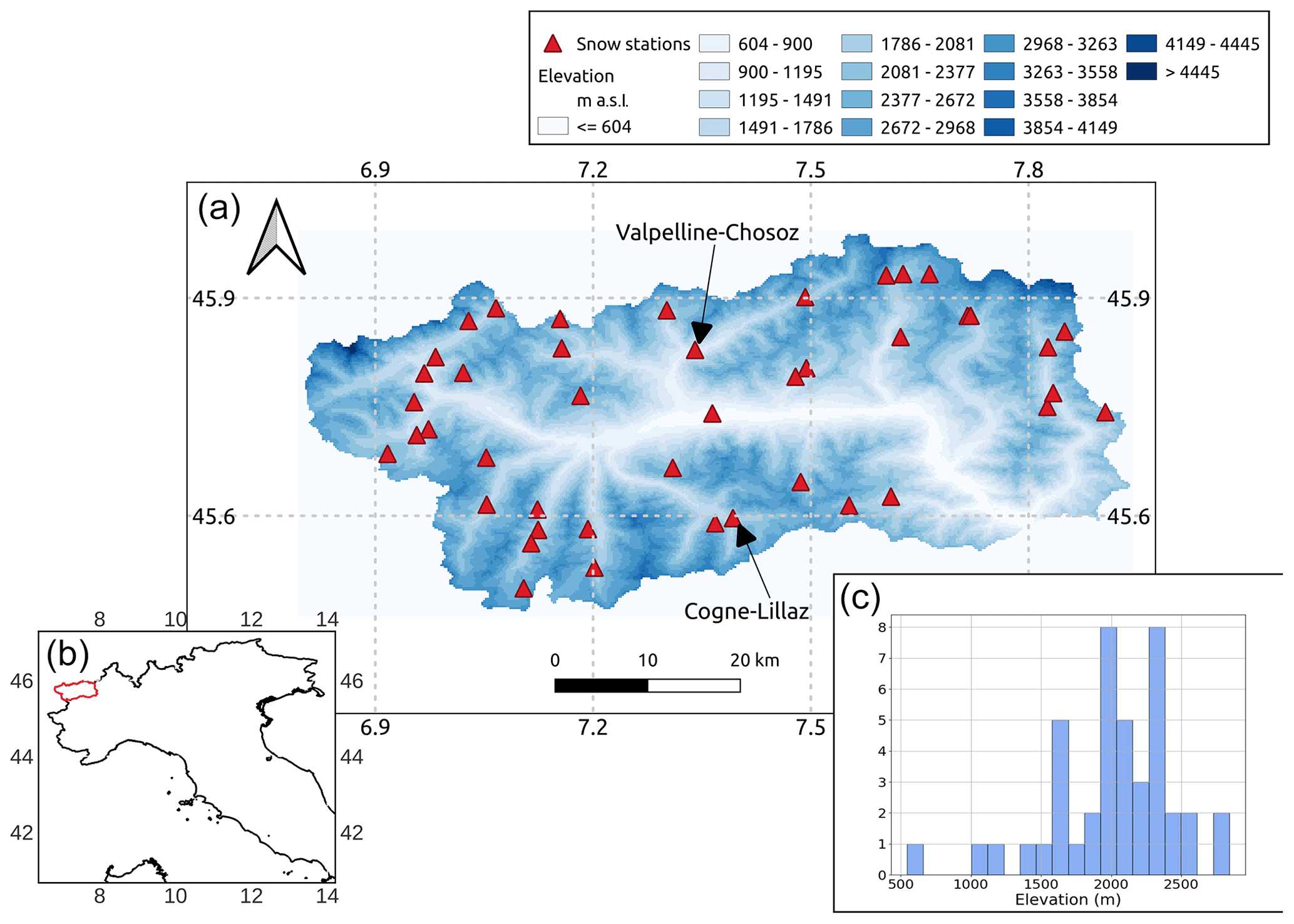
Figure 1Considered snow-depth sensor data across Aosta Valley (see the bottom-left corner for the location of this study region in Italy). The two snow-depth sensors of Chosoz (Valpelline) and Lillaz (Cogne) were used in Sect. 4.3. The histogram in the bottom-right corner of this figure reports the frequency distribution of the elevation of the Aosta Valley sensors.
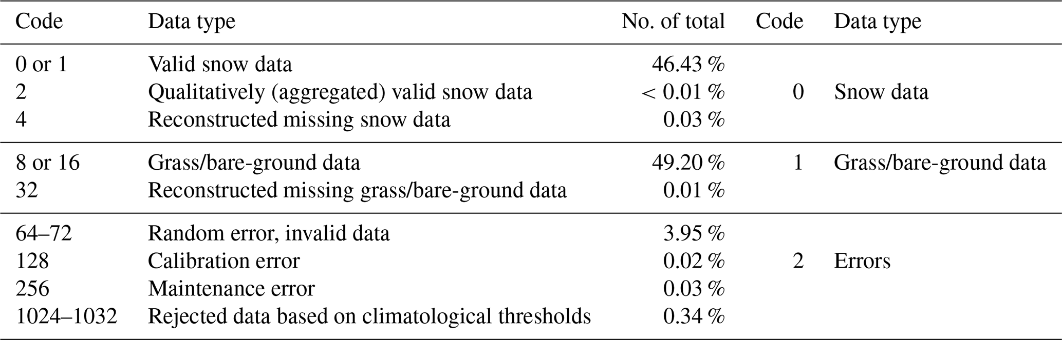
Each data record in this dataset was subject to visual screening by expert hydrologic forecasters during periodical QA/QC manual data processing, with the goal of discriminating random and systematic errors from actual snow-depth measurements. This manual processing follows well-established practices in the field, including crosschecking with concurrent weather (e.g., air temperature, precipitation, relative humidity) and nearby sensors (Avanzi et al., 2014, 2020). As a result, each data point came with a quality code (Table 1): data with code 0 or 1 are valid snow cover data, codes 2 or 4 are for missing data reconstructed from trends or aggregated from different time resolutions, codes 8 and 16 are grass or bare ground, code 32 denotes reconstructed grass data, and codes 64 to 256 denote a variety of flags for random and instrumental errors; codes 1024–1032 refer to data classified as invalid after a preliminary procedure based on fixed thresholds (introduced in 2018). While the dataset includes some reconstructed data, these are only 0.03 % of the whole dataset, which means they do not affect our analyses.
In this work, we reduced the number of classes to 3 by aggregation: correct snow depth, identified with code “0”; grass or bare ground, identified with code “1”; and random errors, identified with code “2”.
Table 1Snow-depth data classification system developed by the Functional Center of Aosta Valley.
2.2 Other Italian data
The validation dataset across the rest of Italy comprises hourly data from 27 ultrasonic depth sensors, randomly chosen among the ∼300 Italian automatic snow-depth sensors available outside Aosta Valley. These 27 snow-depth sensors were chosen based on a geographical-diversity criterion to guarantee heterogeneity, especially with regard to the Aosta Valley data (Fig. 2). This second dataset includes data from 3 years – 2018, 2020, and 2022 – which were chosen due to their significantly different accumulation patterns (deep snowpacks in 2018, somewhat average snowpacks in 2020, and extraordinarily low snowpacks in 2022; see Avanzi et al., 2023). No prior processing was available for these data; thus we proceeded with our own manual classification to assign codes as in Table 1. The procedure included visual screening, checks on seasonality to detect snow vs. grass, and a comparison with measurements from nearby sensors (Avanzi et al., 2014, 2020).
Italy (301×103 km2) is a topographically and climatically complex region. Its main mountain chains, the Alps and the Apennines, are among the highest peaks in Europe. Partially snow-dominated regions like the Po River basin or the central Apennines have high socioeconomic relevance (Group, 2021). The Italian climate presents a considerable variability from north to south. According to the Köppen–Geiger climate classification (Beck et al., 2018), in the Alps the climate is humid and continental. Central Italy, alongside the Apennine chain, is characterized by a warm, temperate, Mediterranean climate with dry, warm summers and cool, wet winters. In Southern Italy, where the climate is still a warm temperate, Mediterranean climate, winters are mild, with higher humidity and higher temperature during summer. Concerning snow-cover distribution, accumulation across the Alps is generally higher and more persistent than across the Apennines, where it is spatially more limited and more variable from one season to the others (Avanzi et al., 2023). Rivers draining from the snow-dominated Alps and a handful of basins draining from the central Apennines host the vast majority of snow water resources across the Italian territory. In particular, the Alpine water basins host nearly 87 % of Italian snow. The central Apennines accumulate about 5 % of the national mean winter SWE, leaving the remaining 8 %–9 % scattered across the remaining basins over the territory. Intraseasonal melt, expected in a Mediterranean region, is a common feature in sites where cold alpine and maritime snow types coexist like the Apennines (Avanzi et al., 2023).
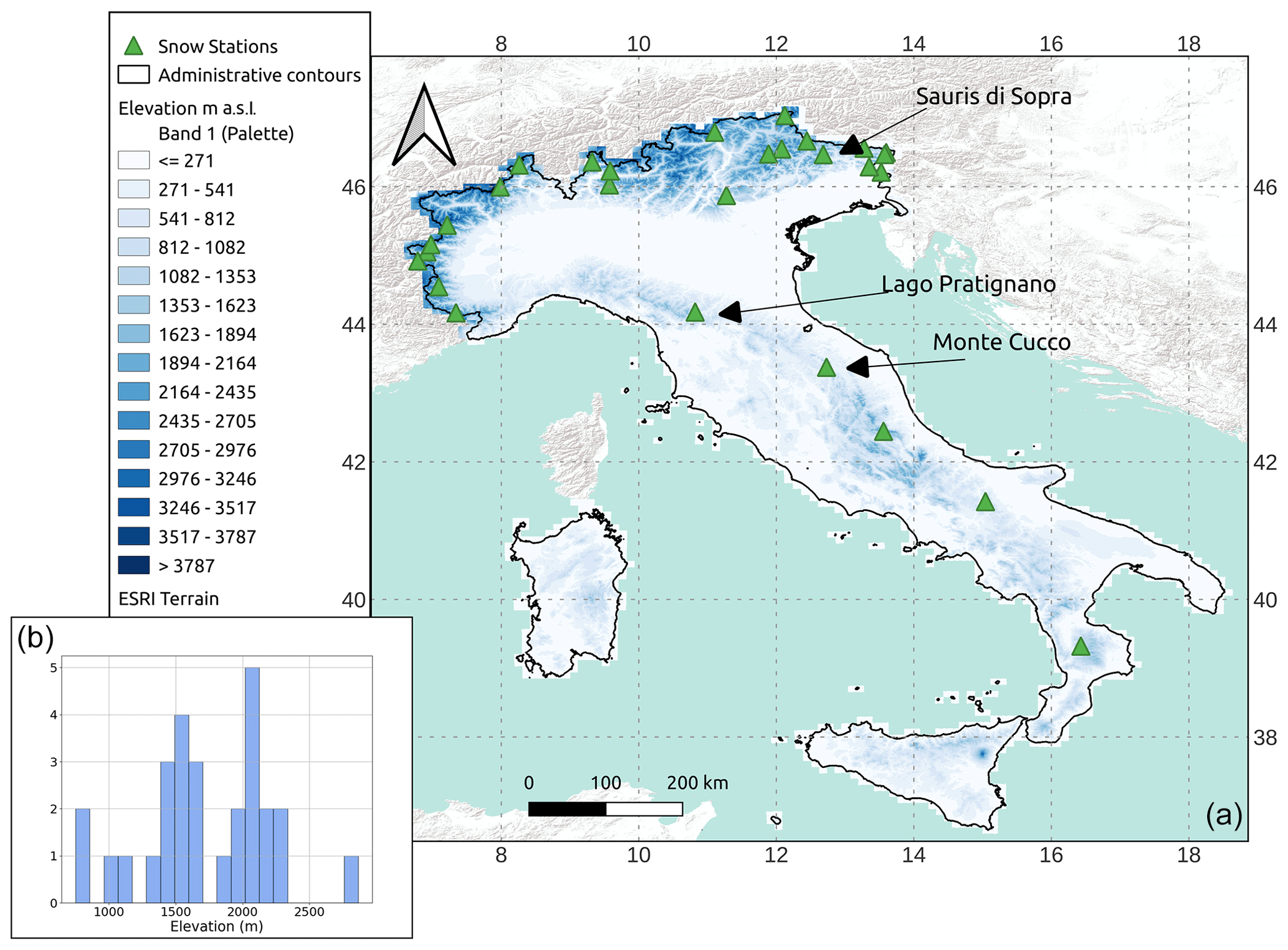
Figure 2(a) Considered snow-depth sensor data across the rest of Italy. (b) Frequency distribution of the elevation of these sensors. Three black arrows indicate the location of three snow-depth sensors used in Sect. 4.5.
3.1 Random forest: background
Among all machine learning approaches, we chose random forest due to its benchmarking nature as well as its simplicity of use (Tyralis et al., 2019), as proven by an increasing number of studies proving the effectiveness of random forest as a classifier or regressor algorithm. For instance, Desai and Ouarda (2021) developed a flood frequency analysis based on random forest, which proved to be equally reliable but more efficient than more complex models; Park et al. (2020) developed a random forest classifier for sea ice using Sentinel-1 data; random forest proved to be efficient in big data environments (Liu, 2014); recently, Ponziani et al. (2023) proved the efficiency of random forest over other machine learning algorithms, developing a predictive model for debris flows that could be experimentally implemented in the existing early warning system of the Aosta Valley. In the context of snow data, Meloche et al. (2022) proved the ability of a random forest algorithm to predict snow-depth distribution from topographic parameters with a root mean square error of 8 cm (23 %) in western Nunavut, Canada. In particular, the algorithm object of the present study is a random forest classifier, an ensemble classifier based on bootstrap aggregation, and random features selection.
A random forest is an ensemble of decorrelated decision trees that are allowed to grow and vote for the most popular class (Breiman, 2001). The growth of each tree in the ensemble is governed by randomness, proven to be a performance enhancer. Randomness is given by two randomization principles: bagging and random feature selection. According to the bagging principle, a large number of relatively uncorrelated trees, each built using a split sample of n dimensions retrieved from the entire training dataset of size m, operate as a committee; this ensemble is proven to outperform any of the individual constituent trees. Therefore, the class definition, made by averaging the scores of each tree, is mildly affected by the weight of misclassification done by less performant trees. Furthermore, instead of splitting a node searching for the most important feature (i.e., predictor), a random forest uses the best one among a random subset of features, performing random feature selection and thus increasing the performances. Randomness injection minimizes correlation across trees and reduces variance and overfitting, increasing stability (Breiman, 2001). Our algorithm was implemented using scikit-learn Version 0.20.1, a Python software programming platform, using the class RandomForestClassifier.
3.2 Random forest development
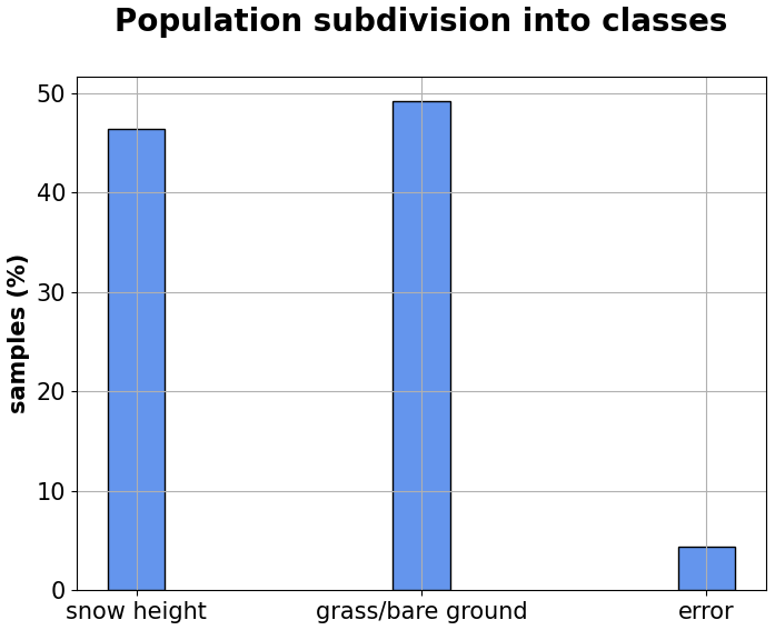
To train the random forest, we used the Aosta Valley classified dataset. Based on data frequency (Fig. 3), this is a typical imbalanced dataset where class distribution is skewed or biased towards one or a few classes in the training dataset (Kuhn and Johnson, 2013).
In this framework, data belong either to majority or minority classes. The majority classes are the classes with a larger number of observations, while the minority classes are those with comparatively few observations. In this case, the number of data classified as random errors (code 2) is significantly lower than the number of data from category 0 (snow height) or category 1 (grass/bare ground). Thus, classes 0 and 1 were defined as majority class, while class 2 was defined as minority class.
Class imbalance can severely affect the classification performance (Ganganwar, 2012; Ramyachitra and Manikandan, 2014) and therefore requires a preprocessing strategy. To this end, acknowledging the work of Ponziani et al. (2023) in which no clear evidence of outperformance of any such strategy was shown, we performed an oversampling of the minority class by selecting examples to be duplicated and then added to the training dataset; we used the class RandomOverSampler from the package imbalanced-learn version 0.8.1. To decrease the computational effort that may have stemmed from this oversampling procedure (Branco et al., 2016), a representative sample of 1.3×10⁶ measurements was taken from the entire dataset prior to the oversampling of the minority class for random forest training. This sample was proven to be representative of the entire dataset distribution (approximately 5.5×10⁶ data points) by performing a two-sample Kolmogorov–Smirnov test, with a significance level equal to 0.05.
After the oversampling procedure, a sample of 1.9×10⁶ oversampled measurements (including both the majority and the oversampled minority classes) was used to train the random forest. From the remaining not oversampled dataset, an independent test sample of 4.8×10⁵ measurements was randomly selected. As a result, a train and test split share of 80 % training and 20 % testing was used, in agreement with current standards in machine learning problems (Harvey and Sotardi, 2018).
When dealing with an imbalance classification, standard evaluation criteria focusing on the most frequent classes may lead to misleading conclusions because they are insensitive to skewed domains (Branco et al., 2016). For example, accuracy, which is defined as the number of correct predictions over the total number of predictions and is a frequently used metrics for classification problems, underestimates the importance of the least represented classes when compared with the majority classes, as it does not take into account data distribution. Adequate metrics need to be used not only for model validation but also for model selection, given that accuracy scores may ignore the difference between types of misclassification errors, as they seek to minimize the overall error. A good metric for imbalance classification must consider overall data distribution, giving at least the same importance to misclassification in both majority and minority classes.
In this paper, we thus used the F measure (Van Rijsbergen, 1979), i.e., the harmonic mean of precision (measure of exactness), defined as the number of true positives divided by the total number of positive predictions, and recall (measure of completeness), defined as the percentage of data samples that a machine learning model correctly identifies as belonging to a class of interest out of the total samples for that class.
The harmonic mean is the reciprocal of the arithmetic mean and tends to mitigate the impact of large outliers while aggravating the impact of small ones since it tends strongly toward the least represented elements.
Fβ (the so-called F measure) is defined as
We set β=1 to give equal importance to precision and recall.
The metrics of precision and recall were used to characterize the performance of the random forest for each class separately. Then macro-averages of both measures were computed to characterize the multi-class performance. A macro-average is the arithmetic mean computed giving equal weight to all classes and is used to evaluate the overall performance of the classifier.
The performances of the trained random forest algorithm were tested on the 20 % test dataset using the model in prediction and comparing the model's classification with that of the expert forecasters. Validation was also performed by applying the final algorithm on the 3 years of data from the rest of Italy (Sect. 2.2).
We chose as candidate predictors (features) of our random forest a collection of meteorological, topographic, and temporal variables that are known to influence snow accumulation and melt, thus mimicking the decision process made by experts when assigning a classification code. These features include snow-depth values themselves, elevation, aspect, concurrent air temperature, incoming shortwave radiation, total precipitation, wind speed, relative humidity, and the day of the year. Feature values were extracted for each data point in both the Aosta Valley and the rest-of-Italy samples using available geographic information and weather maps operationally developed by the CIMA Research Foundation (see Avanzi et al., 2021, for Aosta Valley and Avanzi et al., 2023, for other Italian data).
A feature importance analysis was also performed. Importance was calculated using the attribute “feature importance” of the class RandomForestClassifier in sklearn.ensemble (Pedregosa et al., 2011). The ranking is driven by each feature contribution to a decrease in impurity over trees.
A set of hyperparameters were optimized through a combination of automatic, random searching, and further manual tuning to reduce overfitting, while ensuring good F1 scores and reliable training times for the Aosta Valley dataset. The parameters that were tuned in this work were the number of estimator (namely, the number of trees in the forest), the maximum depth (namely, the maximum number of levels in each decision tree), the minimum sample leaf (namely, minimum number of data points placed in a node before the node is split), and the minimum sample split (namely, minimum number of data points needed to split an internal node). Others default hyperparameters were not modified.
In addition to the general training strategy above, a random forest algorithm was also trained using the Aosta Valley dataset separately for each year, with 80 % of the data used in training and then an out-of-bag validation with the remaining 20 % of the same year of data. The aim of this further test was to investigate the possible correlation between the performance of the classification by the random forest algorithm and annual weather characteristics. For each year, the F1 score for the test sample was analyzed against annual mean values of features used for the classification, computing correlation factors.
Finally, we mapped classification results as a function of feature values to shed light on the decision process taken by the random forest in classifying snow vs. grass/bare ground vs. random errors and how they relate to the original classification by operational forecasters.
4.1 Training and test performances: Aosta Valley
The macro-averaged F1 score of classification for the Aosta Valley dataset during the testing phase was 0.96, with a precision value of 0.97 and a recall of 0.95 (Fig. 4a). In detail, the random forest scored 0.99 in both precision and recall for the classification of snow data. In the classification of grass/bare ground, recall was maximum (1), with a precision of 0.99. Lower values were obtained in the classification of random errors, with a recall of 0.86 and a precision of 0.93, resulting in an F1 score of 0.89. Most of the snow-depth data and grass/bare-ground data were correctly classified (45.94 % and 46.45 %; 49 % and 49.19 %), while a comparatively large sample of error data that was misclassified as snow (0.50 % and 4.43 %; Fig. 4b). Overall, the model resulted in being equally precise and robust in snow and grass/bare-ground classification, while the precision and recall of the random-error class were lower compared to the other two classes (F1 score for snow and grass/bare-ground classes of 0.99 and F1 score for random-error classes of 0.89). As a whole, the model tested in Aosta Valley proved to be slightly more precise than robust (precision 0.97, recall 0.95).
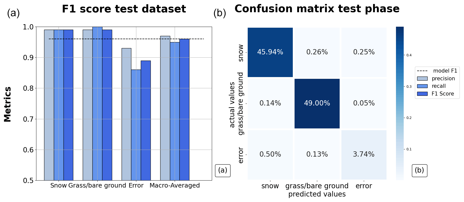
Figure 4(a) Model performances in prediction mode for the test dataset in Aosta Valley. Each set of columns reports the values of precision, recall, and F1 score for the three classes, while the last group on the right shows the macro-averaged values referring to the random forest performances as a whole. The dashed black line is a reference for the macro-averaged F1 score of the random forest. (b) Confusion matrix.
In order to identify recurring patterns in snow cover and grass cover classification during the hydrological year, we visually screened results of the random forest classifier for all data and hydrological years. Figure 5 reports examples for two snow-depth sensor locations (October 2016 to September 2017), which were randomly selected from the entire pool of 43 snow-depth sensors throughout 18 years of the Aosta Valley domain. Note that we removed samples used for the random forest training. We found an expected tendency of the random forest to misclassify snow as grass/bare ground during transitional periods at the beginning and at the end of the snow season (Fig. 5a2), especially when snow cover and grass height are comparable (Fig. 5b2 and b3). Moreover, the random forest sometimes misinterprets settling during the snow period.
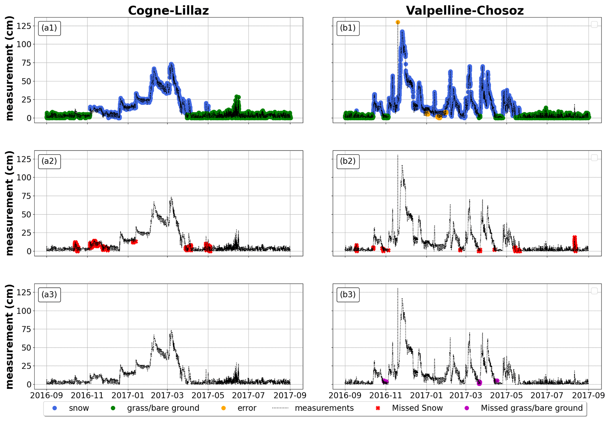
Figure 5Application of random forest on two Aosta Valley snow-depth sensors locations from October 2016 to September 2017. The first row displays the samples of snow height, grass/bare ground, and error correctly classified by the model. In blue are the correctly classified snow samples, in green the correctly classified grass samples, and in orange the correctly classified errors. The second row shows misclassified snow height in red, and the third row reports misclassified grass/bare-ground samples in purple. Data refer to a hydrological year.
4.2 Model configuration
The best set of parameters for the development of the random forest resulted in a number of estimators equal to 500, a maximum depth of 40, a minimum sample leaf equal to 1, and a minimum sample split equal to 2. The choice of the best set of features was initially driven by the F1 macro-average obtained on the test set (Table 2, featuring combination sets from T1 to T7); then, training time was also considered as a discriminant (+10 min for T6 compared to T7). Hence, the set of features selected as the best consisted of the snow-depth record measured by the snow-depth sensor, elevation, aspect, concurrent air temperature, incoming shortwave radiation, cumulative precipitation, relative humidity, and the day of the year to capture seasonality (Table 2, set T7). Regarding elevation and aspect, previous studies have shown that geographic location and elevation indeed contribute to improving machine learning model performance (Bair et al., 2018).
Table 2F1 scores for a variety of tests used to identify the best feature combination for the random forest algorithm. T7 was then selected as the best option in terms of features.
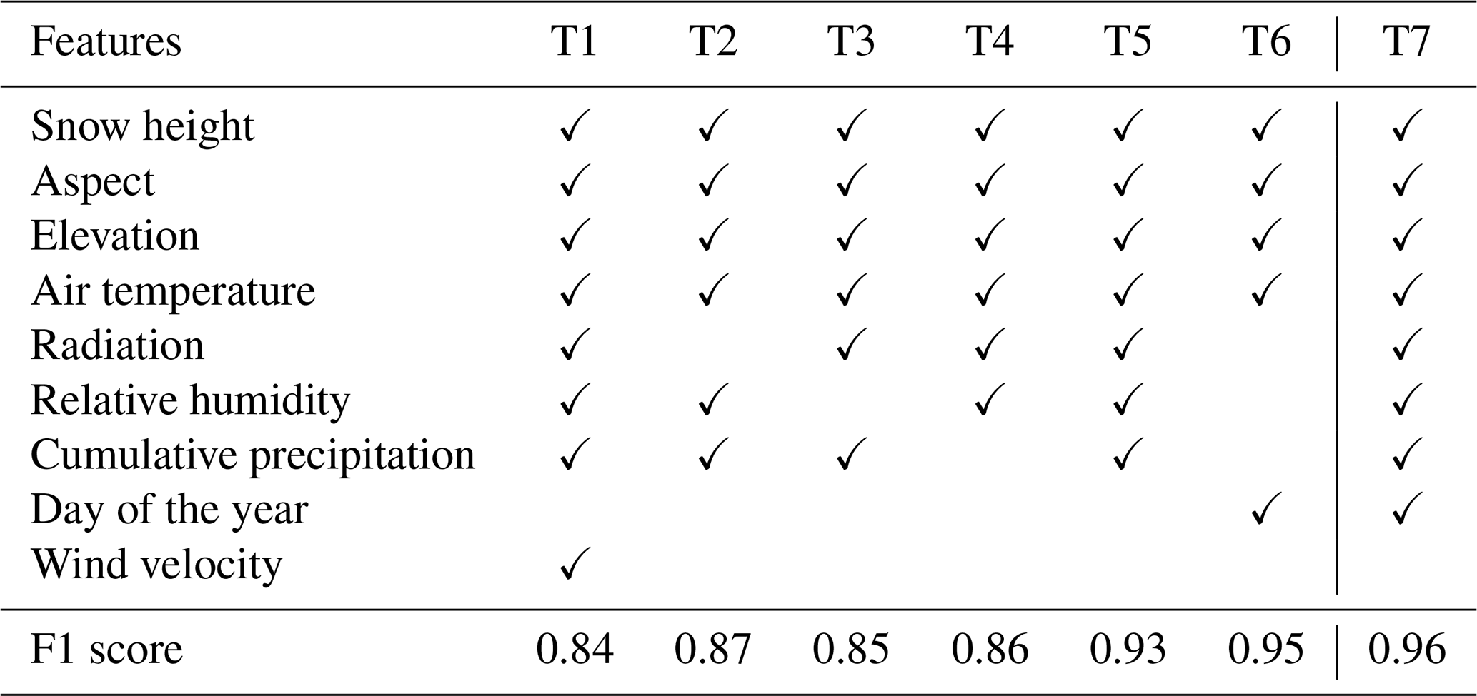
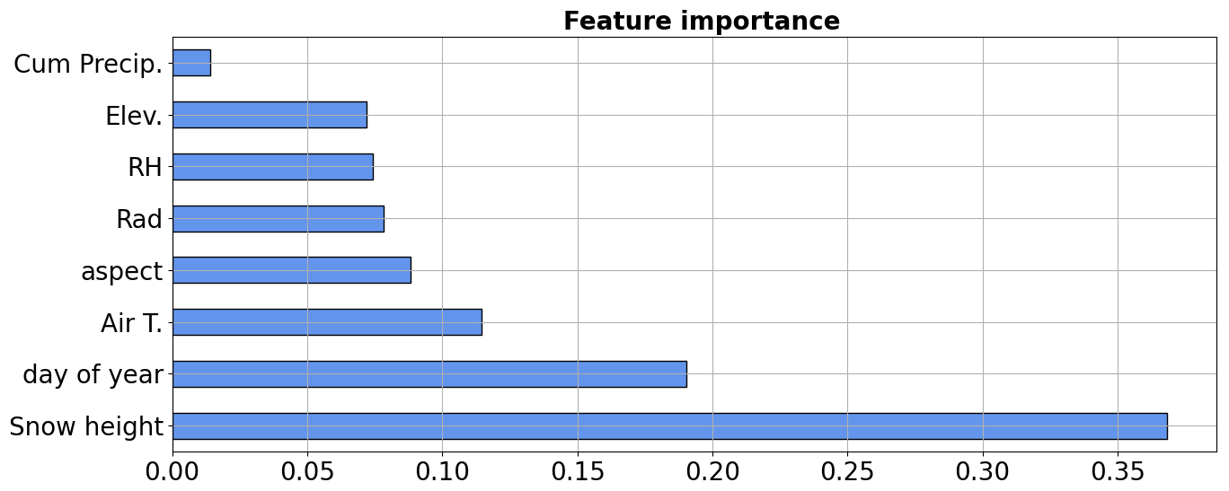
Figure 6Feature importance for the random forest classification procedure in Aosta Valley. The dimensionless values, along the x axis, sum up to 1; the higher the value, the more important the feature is in the definition of the class. Cum Precip.: cumulative precipitation; Elev: elevation; RH: relative humidity; Rad: radiation; air T: air temperature.
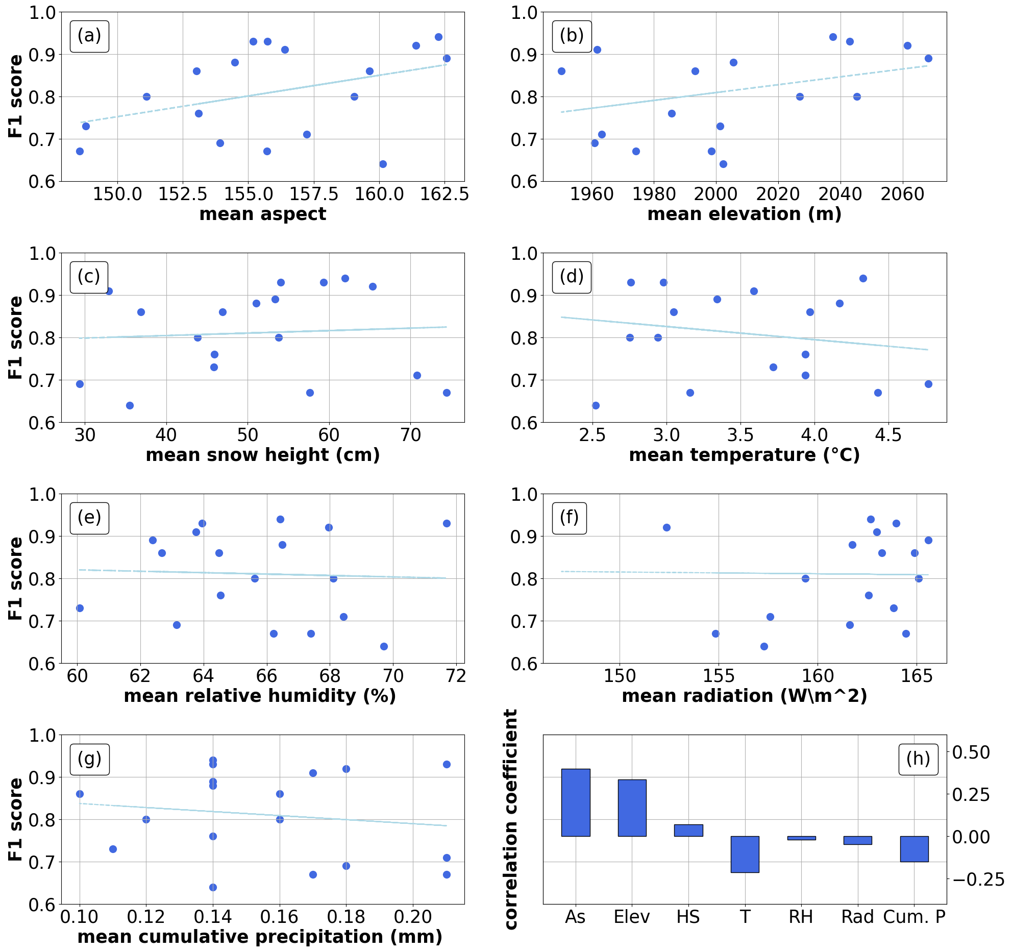
Figure 7Annual F1 score correlated with mean annual feature values. The y axis reports the F1 score macro-averaged for each year, while the x axis shows the values of annual mean for each feature. The straight blue line indicates a linear regression. The last plot indicates the correlation coefficient between single features and F1 score.
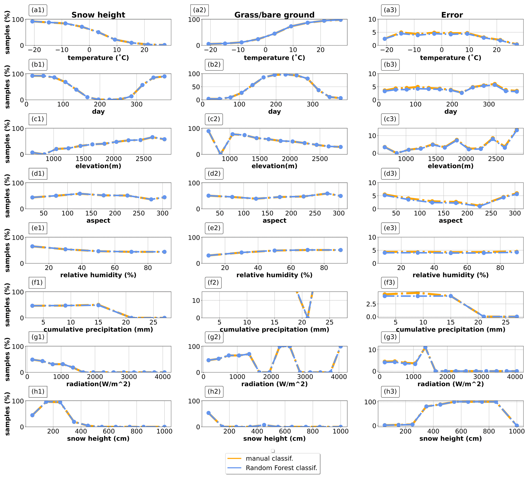
Figure 8Classification results as a function of feature values: the left is for snow classifications, the center is for grass/bare-ground classifications, and the right is for random-error classifications. Orange is the human-made classification, and blue is the classification performed by the random forest. The x axis reports feature values, while the y axis reports the percentage of classification on the total. The plots refer to the test sample in Aosta Valley, it being representative of the entire residual dataset. Data are normalized over the total sample size.
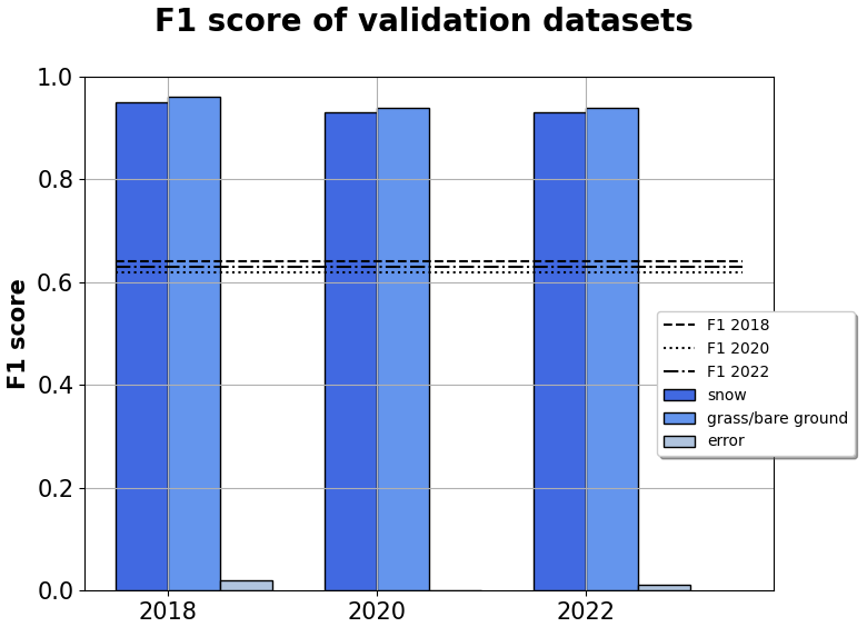
Figure 9Classification performance on the 27 stations across the rest of Italy. The columns grouped along the x axis are the F1 scores for snow, grass/bare ground, and random-error classes subdivided by year. The y axis reports the dimensionless values of each scoring metric. The straight lines are the F1 scores macro-averaged for each year.
Feature importance (Fig. 6) suggested that measured snow depth itself (regardless of whether is represents actual snow depth, grass, bare ground, or random errors) was the most important feature in our random forest, followed by the day of the year, air temperature, and aspect. Radiation, relative humidity, and elevation scored similarly, while total precipitation was the least important feature. Feature importance results followed a somewhat intuitive ranking, similar to human perception. For example, the model gave high importance to snow depth, likely replicating the concept of a “plausible range” of snow depth as opposed to grass, bare ground, or random errors. Seasonality (expressed as day of the year and air temperature) was the second most influencing factor, likely mimicking the concept of a “plausible” period for snow on the ground. Aspect and elevation were less influential, which is likely because of the comparatively small size of the Aosta Valley study region.
It is important to acknowledge that correlation among features and multi-collinearity are problematic for feature importance and interpretation in a random forest. Features importance may spuriously decrease for features that are correlated with those selected as the most important (Strobl et al., 2007). On the other hand, Hastie et al. (2009) point out that the predictive skill of the algorithm is relatively robust to correlations thanks to de-correlation factors involved in bootstrapping. Indeed, even features of low importance may drive the decision process of the algorithm (Avanzi et al., 2019). In our case, we chose to use all the features after verifying the lack of correlations across features below −0.5 or above +0.5.
4.3 F1 correlation with annual climate
Annual mean feature values showed low or negligible correlation coefficients with the annual F1 score (Fig. 7, with removal of training data points). All correlation coefficients were statistically tested, and no correlation was found (p value between −0.21 and 0.40 for all the features).
4.4 Mapping the decision process
Analysis of the random forest decision process highlighted consistency with the classification procedure by expert forecasters, as well as agreement with the expected decision process behind the human-made classification, despite a general underestimation of the number of random-error samples (Fig. 8).
The frequency of data classified as snow decreased with increasing temperature, as expected and in agreement with the original expert classification (Fig. 8a1). Simultaneously, the frequency of data classified as grass/bare ground increased with temperature (Fig. 8a2), again as expected due to the progressive melt and snow disappearance as temperature increases. Regarding random errors, the random forest underestimated their frequency up to 10 ∘C, while automatic and human-made classifications were more comparable in frequency above that temperature threshold (Fig. 8a3).
Considering the day of the year, most snow classifications occurred at the beginning and at the end of the calendar year (thus, in winter); this proved to be consistent between the random forest and the human classification (Fig. 8b1), with then a shift towards the grass/bare-ground class in summer (Fig. 8b2). Overall, we found an underestimation of random-error samples throughout the year, especially in the first 150 d of the year (Fig. 8b3).
The number of data classified as snow progressively increased with elevation (Fig. 8c1), while the number classified as grass/bare-ground decreased with elevation (Fig. 8c2) consistently between the random forest and the original dataset. The frequency of random-error classifications generally matched the human classification, except for an underestimation around 2500 m (1 % of misclassified samples) (Fig. 8c3).
When looking at aspect, both the automatic and human-made snow vs. ground-soil classification were related to local climate. For example, they both classified more snow than grass across southern slopes (between 50 and 251∘), where precipitation is generally more abundant due to seasonal circulation from the Gulf of Genoa (Fig. 8d1 vs. d2; see Rudari et al., 2005; Brunetti et al., 2009). On the other hand, grass classifications increased on north-facing slopes (from 250 to 351∘), likely because these areas are exposed to naturally more humid conditions. Overall, the model underestimated the frequency of random-error classification along all aspects.
As for the other, less important features, they generally showed a negligible influence on the decision process. The only clear exception was relative humidity, since we found a progressive decrease in snow classifications as relative humidity increased (Fig. 8e1), coupled with an increase in the grass/bare-ground classification (Fig. 8e2).
Finally, considering measured snow depth (by far the most important feature)), the model correctly classified all values above 400 cm as random errors, correctly matching the human classification (Fig. 8h3). This is due to an instrumental limit given by the height of the sensor from the ground in this study region. Given that snow depth is the most important feature in driving the classification problem, we found a perfect match between model and human classifications (Fig. 8h1 and h2).
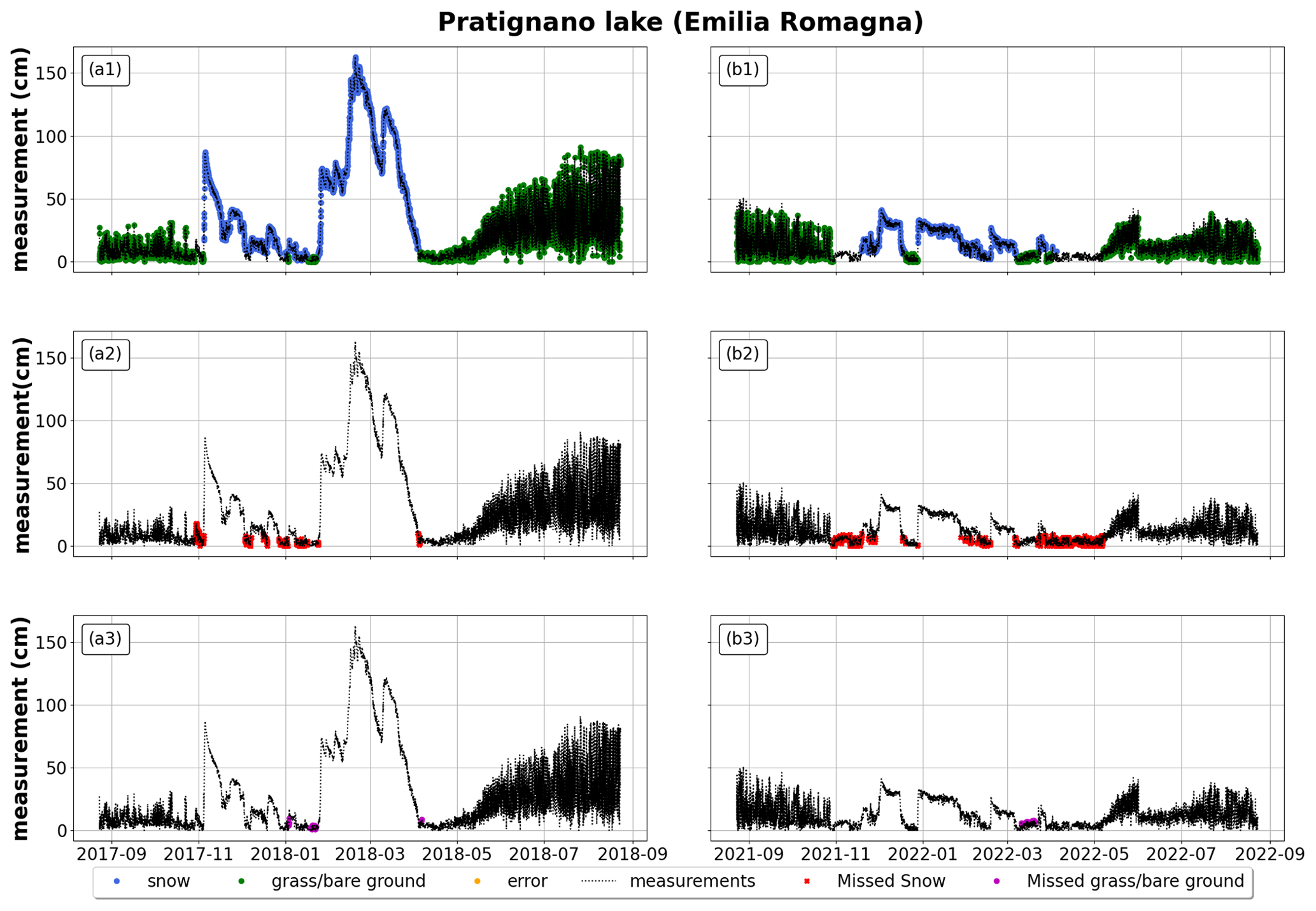
Figure 10Example of application of the random forest to an Italian station (Lago Pratignano, Emilia Romagna). (a1–a3) October 2017 to September 2018; (b1–b3) October 2021 to September 2022. The first row reports the correct classification of snow, grass/bare ground, and random errors (blue for snow depth, green for grass/bare ground, orange for random errors); the second row reports misclassified snow depth (in red); and the third row reports misclassified grass/bare ground (in purple). All plots also report measured snow depth in black (whether it represents actual snow depth, grass/bare ground, or random errors).
4.5 Validation on the rest-of-Italy sample
The application of the random forest on the 27 ultrasonic snow-depth sensors from the rest of Italy showed a surprising robustness in the classification of snow depth and grass/bare ground, with F1 score values between 0.93 and 0.96 across the 3 years. The performances of the random forest on the classification of both snow samples and grass/bare-ground samples proved to be comparable to the ones already noted in Aosta Valley; a severe reduction in performance was registered in the detection of random errors, for which the F1 score was below 0.05 in every year. We explain this as potentially due to the fact that we operated our own classification of this dataset, with an inevitably different subjectivity to that used by the expert forecasters in Aosta Valley; this is particularly impactful for random errors due to their smaller frequency in the sample (error sample frequency: 0.36 % in 2018, 0.92 % in 2020, 0.52 % in 2022).
Results of model application for 2 years at the exemplary station of Pratignano (Fig. 10a2 and b2) suggested a better performance for the model in cases of higher snow depth. In other words, the model better distinguished snow from grass or bare ground when their heights were less commensurable, hence the slightly better performance in a year with higher snow depth (F1 score in 2018: 0.95 for snow and 0.96 for grass/bare ground; F1 score in 2022: 0.93 for snow and 0.94 for grass/bare ground). This example also showed a recurring tendency to confound snow and grass at the beginning and at the end of the season, as already noted in Aosta Valley. Considering grass classification (Fig. 10a3 and b3), we also found a tendency to misclassify snow and grass during periods of intraseasonal melt. Two other examples of the application of the random forest to exemplary sites can be found in the Appendix. We chose to show a snow-depth sensor located in the Apennines (Fig. A1) and one located in northeastern Italy (Fig. A2) to better portrait snow regimes and random forest performances across Italy.
Due to the central role that snow plays in the global water cycle (Flanner et al., 2011; Beniston et al., 2018), snow measurements have proven to be essential in the development of trustworthy numerical prediction models and snowpack models (Horton and Haegeli, 2022). In this framework, high-resolution measurements not only include meaningful information, for example related to snowfall intensity and amount (Lehning et al., 2002b, a) or snowmelt patterns (Malek et al., 2017; Zhang et al., 2017), but also embed a variety of noise sources that hamper their use in operations unless intensive QA/QC is performed (Avanzi et al., 2014). The overarching hypothesis of this paper was that a random forest classifier could replace expert manual checking and automatically process snow-depth high-resolution measurements from ultrasonic snow-depth sensors and thus add new value to these data for hydrologic practice and research. The main findings of this paper in this regard are threefold.
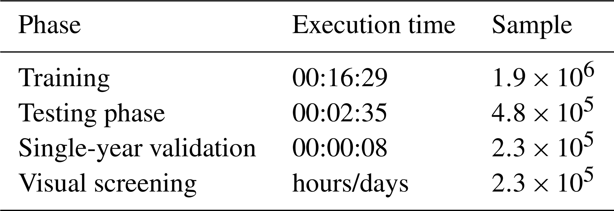
First, the proposed random forest classifier was able to correctly replicate expert-made snow vs. grass/bare-ground classifications, with F1 scores over 90 % for the training–testing case study of Aosta Valley. These results show that the human assessment based on expert knowledge is largely replicable (see Fig. 8), at least for what concerns the classification of snow and grass/bare-ground samples. While intuitively simple in nature, this differentiation is instead complex to automatize due to nonlinearities across climate, snow regimes, vegetation patterns, and topography. Meanwhile, differentiating grass/bare ground from snow bears significant implications with regard to snow-depth assimilation in snowpack models (Bartelt and Lehning, 2002), satellite-data validation using ground-based data (Parajka and Blöschl, 2006; Da Ronco et al., 2020), and a variety of ecological analyses related to snow (Sanders-DeMott et al., 2018). In this regard, our proposed random forest is a pathway towards minimizing this noise and thus accelerating the use of snow-depth data in science and technology by opening the way for a fast, objective, and replicable QA/QC of snow-depth data that could complement existing practices (Avanzi et al., 2014; Bavay and Egger, 2014). Regarding speed, Table 3 shows that applying our random forest of one season's worth of data takes about 8 s as opposed to an estimate of hours for visual screening based on our own experience.
Second, the algorithm proved to be equally robust and reliable in an independent application across the rest of Italy, at least for what concerns the snow vs. grass/bare-ground classification (F1 scores above 90 % for this larger domain). We explain this outcome as being due to our random forest including all features of the Sturm and Liston (2021) snow classification, such as air temperature and precipitation or proxies thereof (elevation for wind speed). At the same time, the vast majority of Italian sites falls between the maritime and the montane-forest snow-climatology classes, with only a small portion of tundra snow at very high, inner-Alpine elevations (Sturm and Liston, 2021). In other words, our testing sample might be quite homogeneous with regard to snow climatology, and testing over other regions would still be helpful.
Third, we found little to no sensitivity to snow-season climatology (Fig. 7), including temperature or mean snow depth. This result may point to our random forest being robust to different climatic regimes, including recent dry and warm snow droughts (Hatchett and McEvoy, 2018; Toreti et al., 2022; Koehler et al., 2022) and future climate change (Beniston et al., 2018). However, long-term climatic shifts will also bring about modifications to vegetation patterns (Cannone et al., 2008) and so changes in the expected seasonality of grass vs. snow, as well as changes to the “expected” snow depth during winter (Marty et al., 2017). Both aspects will need further testing in areas with different climates.
It is worth mentioning that, although the choice of these validation datasets allowed us to test the spatial extrapolation abilities of the random forest, a full evaluation of the spatiotemporal extrapolation skills was not achieved. The algorithm was trained on all the available years, with a standard out-of-bag validation. This was performed in an effort to maximize the number of training points and climate variability in our training sample. Thus no year was withdraw to reduce the impact of impoverishment of the sample on the least represented class of random errors.
One critical aspect of our results is the frequently reported underestimation of random errors, like spikes, particularly across the rest-of-Italy data. This may be seen as the natural consequence of our samples being inherently imbalanced towards snow or grass/bare-ground measurements (see Fig. 3). Moreover, random errors are by definition hard to predict, with the only documented pattern of snowflake interference within the field of view of ultrasonic snow-depth sensors (Avanzi et al., 2020). A potential solution in this regard is for future applications to specifically target the classification of random errors by either including more samples of this class or simply extending the analysis to more data. The use of more data is likely the most straightforward option to detect rare random errors. However, other options may prove to be effective. In light of this, the proposed algorithm may be coupled with classical QA/QC procedures imposing a priori thresholds, like those already proposed by Bavay and Egger (2014). Such procedures could, e.g., help with the detection of spikes in data using climatological snow-depth thresholds for maximum values.
In recent years, deep learning has proven successful in dealing with many complex tasks (Camps-Valls et al., 2021). Future research questions may investigate the ability of other algorithms in this classification problem, such as neural networks, which are able to deal with time series and incorporate memory features. One concrete example in this regard is a recurrent neural networks or LSTM (long short-term memory). In particular, it would be important to explore the performances of such algorithms in dealing with the recognition of the error class. In any case, the small proportion of random errors over the much more influential systematic issue of grass interference makes our random forest a promising component of future QA/QC procedures.
Noise sources in high-resolution snow-depth data severely limit their automatic use in snow models, whether in assimilation or in evaluation mode, thus affecting water management, hydrological forecasting, and emergency preparedness. In particular, snow-depth measurements from ultrasonic sensors are prone to snow vs. grass ambiguity and random noise. Meanwhile, the increasing volume of available data highlights that non-replicable, time-consuming, and error-prone visual screening procedures are increasingly less feasible. Here, we hypothesized that current practices in snow-depth data processing could be improved by training a random forest to replicate expert-knowledge data processing of snow-depth data and so develop an automatic, time-saving quality-checking procedure. The algorithm used is a random forest classifier, a competitive and straightforward approach compared to other machine learning algorithms. Our results show that the proposed random forest is reliable and can generalize on large domains the important detection of snow vs. grass/bare ground (F1 score values above 90 % even in areas outside the original training sample). The algorithm shows little to no sensitivity to snow-season climatology, while it is still exposed to an underestimation of rare random errors that will be the subject of future studies. Our random forest can be readily employed as a component of supervised or unsupervised processing procedures for snow depth.
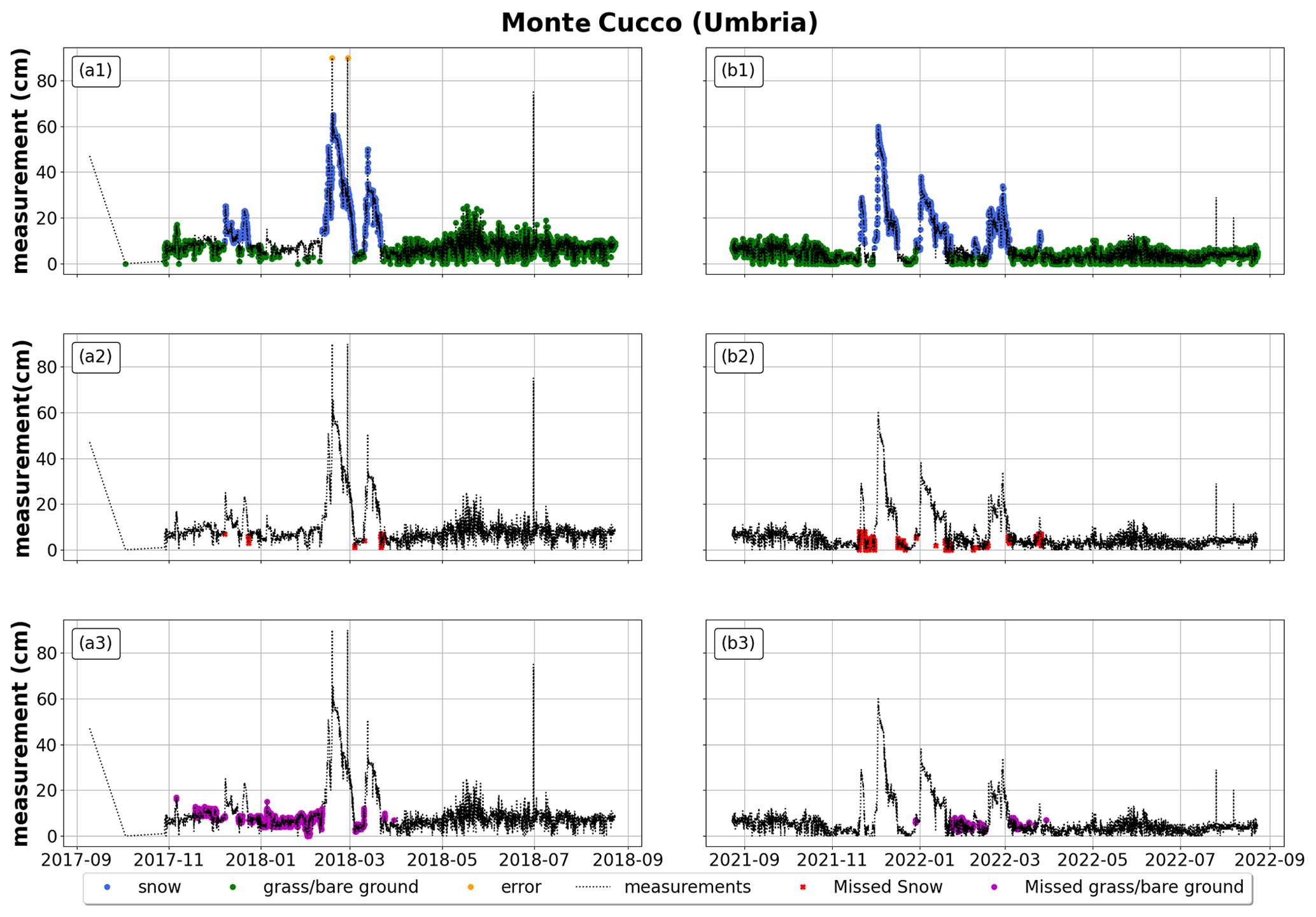
Figure A1For Monte Cucco (Umbria), application of random forest to an Italian station from October 2017 to September 2018 on the left and from October 2021 to September 2022 on the right. The first row reports the correct classification of snow, grass/bare ground, and random errors (blue for snow depth, green for grass/bare ground, orange for random errors); the second row reports misclassified snow depth (in red); and the third row reports misclassified grass/bare ground (in purple). All plots also report measured snow depth in black (whether it represents actual snow depth, grass/bare ground, or random errors).
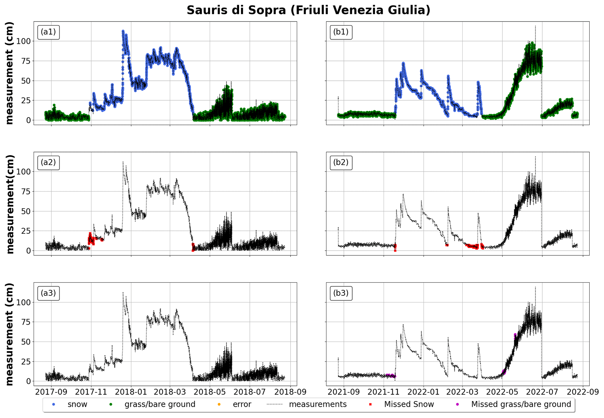
Figure A2For Sauris di Sopra (Friuli Venezia Giulia), application of random forest to an Italian station from October 2017 to September 2018 on the left and from October 2021 to September 2022 on the right. The first row reports the correct classification of snow, grass/bare ground, and random errors (blue for snow depth, green for grass/bare ground, orange for random errors); the second row reports misclassified snow depth (in red); and the third row reports misclassified grass/bare ground (in purple). All plots also report measured snow depth in black (whether it represents actual snow depth, grass/bare ground, or random errors).
Sources of data used are reported in the paper and include the database of the Italian Regional Administrations and Autonomous Provinces.
GB and FA designed and implemented the automatic procedure. DP, HS, and SR developed the human-made classification procedure and provided the labeled data. All authors were involved in discussing the results, reviewing the manuscript, and drafting the final version.
The contact author has declared that none of the authors has any competing interests.
Publisher's note: Copernicus Publications remains neutral with regard to jurisdictional claims made in the text, published maps, institutional affiliations, or any other geographical representation in this paper. While Copernicus Publications makes every effort to include appropriate place names, the final responsibility lies with the authors.
We would like to thank Mirko D'Andrea for his seminal advice during the early stages of this work.
This paper was edited by Guillaume Chambon and reviewed by two anonymous referees.
Avanzi, F., De Michele, C., Ghezzi, A., Jommi, C., and Pepe, M.: A processing–modeling routine to use SNOTEL hourly data in snowpack dynamic models, Adv. Water Resour., 73, 16–29, 2014. a, b, c, d, e, f
Avanzi, F., Johnson, R. C., Oroza, C. A., Hirashima, H., Maurer, T., and Yamaguchi, S.: Insights into preferential flow snowpack runoff using random forest, Water Resour. Res., 55, 10727–10746, 2019. a
Avanzi, F., Zheng, Z., Coogan, A., Rice, R., Akella, R., and Conklin, M. H.: Gap-filling snow-depth time-series with Kalman filtering-smoothing and expectation maximization: Proof of concept using spatially dense wireless-sensor-network data, Cold Reg. Sci. Technol., 175, 103066, https://doi.org/10.1016/j.coldregions.2020.103066, 2020. a, b, c
Avanzi, F., Ercolani, G., Gabellani, S., Cremonese, E., Pogliotti, P., Filippa, G., Morra di Cella, U., Ratto, S., Stevenin, H., Cauduro, M., and Juglair, S.: Learning about precipitation lapse rates from snow course data improves water balance modeling, Hydrol. Earth Syst. Sci., 25, 2109–2131, https://doi.org/10.5194/hess-25-2109-2021, 2021. a, b, c
Avanzi, F., Gabellani, S., Delogu, F., Silvestro, F., Pignone, F., Bruno, G., Pulvirenti, L., Squicciarino, G., Fiori, E., Rossi, L., Puca, S., Toniazzo, A., Giordano, P., Falzacappa, M., Ratto, S., Stevenin, H., Cardillo, A., Fioletti, M., Cazzuli, O., Cremonese, E., Morra di Cella, U., and Ferraris, L.: IT-SNOW: a snow reanalysis for Italy blending modeling, in situ data, and satellite observations (2010–2021), Earth Syst. Sci. Data, 15, 639–660, https://doi.org/10.5194/essd-15-639-2023, 2023. a, b, c, d, e
Bair, E. H., Davis, R. E., and Dozier, J.: Hourly mass and snow energy balance measurements from Mammoth Mountain, CA USA, 2011–2017, Earth Syst. Sci. Data, 10, 549–563, https://doi.org/10.5194/essd-10-549-2018, 2018. a, b
Bartelt, P. and Lehning, M.: A physical SNOWPACK model for the Swiss avalanche warning Part I: numerical model, Cold Reg. Sci. Technol., 35, 123–145, https://doi.org/10.1016/S0165-232X(02)00074-5, 2002. a
Bavay, M. and Egger, T.: MeteoIO 2.4.2: a preprocessing library for meteorological data, Geosci. Model Dev., 7, 3135–3151, https://doi.org/10.5194/gmd-7-3135-2014, 2014. a, b, c, d
Beck, H. E., Zimmermann, N. E., McVicar, T. R., Vergopolan, N., Berg, A., and Wood, E. F.: Present and future Köppen-Geiger climate classification maps at 1-km resolution, Sci. Data, 5, 1–12, 2018. a
Beniston, M., Farinotti, D., Stoffel, M., Andreassen, L. M., Coppola, E., Eckert, N., Fantini, A., Giacona, F., Hauck, C., Huss, M., Huwald, H., Lehning, M., López-Moreno, J.-I., Magnusson, J., Marty, C., Morán-Tejéda, E., Morin, S., Naaim, M., Provenzale, A., Rabatel, A., Six, D., Stötter, J., Strasser, U., Terzago, S., and Vincent, C.: The European mountain cryosphere: a review of its current state, trends, and future challenges, The Cryosphere, 12, 759–794, https://doi.org/10.5194/tc-12-759-2018, 2018. a, b
Berghuijs, W., Woods, R., and Hrachowitz, M.: A precipitation shift from snow towards rain leads to a decrease in streamflow, Nat. Clim Change, 4, 583–586, 2014. a
Branco, P., Torgo, L., and Ribeiro, R. P.: A survey of predictive modeling on imbalanced domains, ACM Computing Surveys (CSUR), 49, 1–50, 2016. a, b
Breiman, L.: Random forests, Machine learning, 45, 5–32, 2001. a, b
Brunetti, M., Lentini, G., Maugeri, M., Nanni, T., Simolo, C., and Spinoni, J.: 1961–1990 high-resolution Northern and Central Italy monthly precipitation climatologies, Adv. Sci. Res., 3, 73–78, https://doi.org/10.5194/asr-3-73-2009, 2009. a
Camps-Valls, G., Tuia, D., Zhu, X. X., and Reichstein, M. (Eds.): Deep learning for the Earth Sciences: A comprehensive approach to remote sensing, climate science and geosciences, John Wiley & Sons, https://doi.org/10.1002/9781119646181, 2021. a
Cannone, N., Diolaiuti, G., Guglielmin, M., and Smiraglia, C.: Accelerating climate change impacts on alpine glacier forefield ecosystems in the European Alps, Ecol. Appl., 18, 637–648, https://doi.org/10.1890/07-1188.1, 2008. a
Da Ronco, P., Avanzi, F., De Michele, C., Notarnicola, C., and Schaefli, B.: Comparing MODIS snow products Collection 5 with Collection 6 over Italian Central Apennines, Int. J. Remote Sens., 41, 4174–4205, https://doi.org/10.1080/01431161.2020.1714778, 2020. a
Desai, S. and Ouarda, T. B.: Regional hydrological frequency analysis at ungauged sites with random forest regression, J. Hydrol., 594, 125861, https://doi.org/10.1016/j.jhydrol.2020.125861, 2021. a
Dettinger, M.: Impacts in the third dimension, Nat. Geosci., 7, 166–167, 2014. a
Ferreira, L. E. B., Gomes, H. M., Bifet, A., and Oliveira, L. S.: Adaptive random forests with resampling for imbalanced data streams, 2019 International Joint Conference on Neural Networks (IJCNN), 14–19 July 2019, Budapest, Hungary, 1–6, 2019. a
Fiebrich, C. A., Morgan, C. R., McCombs, A. G., Hall, P. K., and McPherson, R. A.: Quality assurance procedures for mesoscale meteorological data, J. Atmos. Ocean. Tech., 27, 1565–1582, 2010. a
Flanner, M. G., Shell, K. M., Barlage, M., Perovich, D. K., and Tschudi, M. A.: Radiative forcing and albedo feedback from the Northern Hemisphere cryosphere between 1979 and 2008, Nat. Geosci., 4, 151–155, https://doi.org/10.1038/ngeo1062, 2011. a, b
Ganganwar, V.: An overview of classification algorithms for imbalanced datasets, International Journal of Emerging Technology and Advanced Engineering, 2, 42–47, 2012. a
Group, T. W. B.: Italy-Climatology, https://climateknowledgeportal.worldbank.org/country/italy/climate-data-historical/, last access: 15 September 2023, 2021. a
Harpold, A., Dettinger, M., and Rajagopal, S.: Defining snow drought and why it matters, Eos, 98, 2017. a
Hartman, R. K., Rost, A. A., and Anderson, D. M.: Operational processing of multi-source snow data, Proceedings of the Western Snow Conference, 147, 151, 1995. a
Harvey, H. B. and Sotardi, S. T.: The pareto principle, J. Am. Coll. Radiol., 15, 931, https://doi.org/10.1016/j.jacr.2018.02.026, 2018. a
Hastie, T., Tibshirani, R., Friedman, J. H., and Friedman, J. H.: The elements of statistical learning: data mining, inference, and prediction, vol. 2, Springer, Dept. of Statistics, Stanford University, Stanford, CA, 94305, USA, https://doi.org/10.1007/b94608_1, 2009. a
Hatchett, B. J. and McEvoy, D. J.: Exploring the Origins of Snow Drought in the Northern Sierra Nevada, California, Earth Interactions, 22, 1–13, https://doi.org/10.1175/EI-D-17-0027.1, 2018. a
Horton, S. and Haegeli, P.: Using snow depth observations to provide insight into the quality of snowpack simulations for regional-scale avalanche forecasting, The Cryosphere, 16, 3393–3411, https://doi.org/10.5194/tc-16-3393-2022, 2022. a
Jones, A. S., Horsburgh, J. S., and Eiriksson, D. P.: Assessing subjectivity in environmental sensor data post processing via a controlled experiment, Ecol. Inform., 46, 86–96, 2018. a, b
Koehler, J., Dietz, A. J., Zellner, P., Baumhoer, C. A., Dirscherl, M., Cattani, L., Vlahović, C., Alasawedah, M. H., Mayer, K., Haslinger, K., Bertoldi, G., Jacob, A., and Kuenzer, C.: Drought in Northern Italy: Long Earth Observation Time Series Reveal Snow Line Elevation to Be Several Hundred Meters Above Long-Term Average in 2022, Remote Sens., 14, 6091, https://doi.org/10.3390/rs14236091, 2022. a
Kuhn, M. and Johnson, K.: Applied predictive modeling, vol. 26, Springer, New York, 2013. a
Lehning, M., Bartelt, P., Brown, B., and Fierz, C.: A physical SNOWPACK model for the Swiss avalanche warning Part III: meteorological forcing, thin layer formation and evaluation, Cold Reg. Sci. Technol., 35, 169–184, 2002a. a
Lehning, M., Bartelt, P., Brown, B., Fierz, C., and Satyawali, P.: A physical SNOWPACK model for the Swiss avalanche warning Part II. Snow microstructure, Cold Reg. Sci. Technol., 35, 147–167, 2002b. a
Liu, Y.: Random forest algorithm in big data environment, Comput. Model. New Technol., 18, 147–151, 2014. a
Malek, S. A., Avanzi, F., Brun-Laguna, K., Maurer, T., Oroza, C. A., Hartsough, P. C., Watteyne, T., and Glaser, S. D.: Real-Time Alpine Measurement System Using Wireless Sensor Networks, Sensors, 17, 2583, https://doi.org/10.3390/s17112583, 2017. a
Marty, C., Tilg, A.-M., and Jonas, T.: Recent Evidence of Large-Scale Receding Snow Water Equivalents in the European Alps, J. Hydrometeorol., 18, 1021–1031, https://doi.org/10.1175/JHM-D-16-0188.1, 2017. a
Maurer, T., Avanzi, F., Oroza, C. A., Glaser, S. D., Conklin, M., and Bales, R. C.: Optimizing spatial distribution of watershed-scale hydrologic models using Gaussian Mixture Models, Environ. Model. Softw., 142, 105076, https://doi.org/10.1016/j.envsoft.2021.105076, 2021. a
Meloche, J., Langlois, A., Rutter, N., McLennan, D., Royer, A., Billecocq, P., and Ponomarenko, S.: High-resolution snow depth prediction using Random Forest algorithm with topographic parameters: A case study in the Greiner watershed, Nunavut, Hydrol. Process., 36, e14546, https://doi.org/10.1002/hyp.14546, 2022. a
Parajka, J. and Blöschl, G.: Validation of MODIS snow cover images over Austria, Hydrol. Earth Syst. Sci., 10, 679–689, https://doi.org/10.5194/hess-10-679-2006, 2006. a
Park, J.-W., Korosov, A. A., Babiker, M., Won, J.-S., Hansen, M. W., and Kim, H.-C.: Classification of sea ice types in Sentinel-1 synthetic aperture radar images, The Cryosphere, 14, 2629–2645, https://doi.org/10.5194/tc-14-2629-2020, 2020. a
Pedregosa, F., Varoquaux, G., Gramfort, A., Michel, V., Thirion, B., Grisel, O., Blondel, M., Prettenhofer, P., Weiss, R., Dubourg, V., Vanderplas, J., Passos, A., Cournapeau, D., Brucher, M., Perrot, M., and Duchesnay, E.: Scikit-learn: Machine Learning in Python, J. Mach. Learn. Res., 12, 2825–2830, 2011. a
Ponziani, M., Ponziani, D., Giorgi, A., Stevenin, H., and Ratto, S.: The use of machine learning techniques for a predictive model of debris flows triggered by short intense rainfall, Nat. Hazards, 117, 1–20, 2023. a, b
Ramyachitra, D. and Manikandan, P.: Imbalanced dataset classification and solutions: a review, Int. J. Comput. Business Res., 5, 1–29, 2014. a
Robinson, D. A.: Evaluation of the collection, archiving and publication of daily snow data in the United States, Phys. Geogr., 10, 120–130, 1989. a
Rudari, R., Entekhabi, D., and Roth, G.: Large-scale atmospheric patterns associated with mesoscale features leading to extreme precipitation events in Northwestern Italy, Adv. Water Resour., 28, 601–614, https://doi.org/10.1016/j.advwatres.2004.10.017, 2005. a
Ryan, W. A., Doesken, N. J., and Fassnacht, S. R.: Preliminary results of ultrasonic snow depth sensor testing for National Weather Service (NWS) snow measurements in the US, Hydrol. Process., 22, 2748–2757, 2008. a
Sanders-DeMott, R., McNellis, R., Jabouri, M., and Templer, P. H.: Snow depth, soil temperature and plant–herbivore interactions mediate plant response to climate change, J. Ecol., 106, 1508–1519, https://doi.org/10.1111/1365-2745.12912, 2018. a
Schmidt, L., Schaefer, D., Geller, J., Lünenschloss, P., Palm, B., Rinke, K., and Bumberger, J.: System for automated Quality Control (SaQC) to enable traceable and reproducible data streams in environmental science, Environ. Model. Softw., 169, https://doi.org/10.1016/j.envsoft.2023.105809, 2018. a, b
Strobl, C., Boulesteix, A.-L., Zeileis, A., and Hothorn, T.: Bias in random forest variable importance measures: Illustrations, sources and a solution, BMC bioinformatics, 8, 1–21, 2007. a
Sturm, M. and Liston, G. E.: Revisiting the Global Seasonal Snow Classification: An Updated Dataset for Earth System Applications, J. Hydrometeorol., 22, 2917–2938, https://doi.org/10.1175/JHM-D-21-0070.1, 2021. a, b, c
Toreti, A., Bavera, D., Avanzi, F., Cammalleri, C., De Felice, M., De Jager, A., Di Ciollo, C., Gabellani, S., Maetens, W., Magni, D., Manfron, G., Masante, D., Mazzeschi, M., Mccormick, N., Naumann, G., Niemeyer, S., Rossi, L., Seguini, L., Spinoni, J., and Van Den Berg, M.: Drought in northern Italy – March 2022, GDO analytical report, https://doi.org/10.2760/781876, 2022. a, b
Tyralis, H., Papacharalampous, G., and Langousis, A.: A brief review of random forests for water scientists and practitioners and their recent history in water resources, Water, 11, 910, https://doi.org/10.3390/w11050910, 2019. a
Van Rijsbergen, C.: Information retrieval: theory and practice, in: Proceedings of the Joint IBM/University of Newcastle upon Tyne Seminar on Data Base Systems, vol. 79, 1979. a
Vitasse, Y., Rebetez, M., Filippa, G., Cremonese, E., Klein, G., and Rixen, C.: “Hearing” alpine plants growing after snowmelt: ultrasonic snow sensors provide long-term series of alpine plant phenology, Int. J. Biometeorol., 61, 349–361, 2017. a
Zhang, Z., Glaser, S., Bales, R., Conklin, M., Rice, R., and Marks, D.: Insights into mountain precipitation and snowpack from a basin‐scale wireless‐sensor network, Water Resour. Res., 53, 6626–6641, https://doi.org/10.1002/2016WR018825, 2017. a
Zhong, S., Zhang, K., Bagheri, M., Burken, J. G., Gu, A., Li, B., Ma, X., Marrone, B. L., Ren, Z. J., Schrier, J., Shi, W., Tan, H., Wang, T., Wang, X., Wong, B. M., Xiao, X., Yu, X., Zhu, J. J., and Zhang, H.: Machine learning: new ideas and tools in environmental science and engineering, Environ. Sci. Technol., 55, 12741–12754, 2021. a