the Creative Commons Attribution 4.0 License.
the Creative Commons Attribution 4.0 License.
 | 03 Nov 2023
The impacts of anomalies in atmospheric circulations on Arctic sea ice outflow and sea ice conditions in the Barents and Greenland seas: case study in 2020
Fanyi Zhang
Mengxi Zhai
Xiaoping Pang
Na Li
Arctic sea ice outflow to the Atlantic Ocean is essential to the Arctic sea ice mass budget and the marine environments in the Barents and Greenland seas (BGS). With the extremely positive Arctic Oscillation (AO) in winter (JFM) 2020, the feedback mechanisms of anomalies in Arctic sea ice outflow and their impacts on winter–spring sea ice and other marine environmental conditions in the subsequent months until early summer in the BGS were investigated. The results reveal that the total sea ice area flux (SIAF) through the Fram Strait, the Svalbard–Franz Josef Land passageway, and the Franz Josef Land–Novaya Zemlya passageway in winter and June 2020 was higher than the 1988–2020 climatology. The relatively large total SIAF, which was dominated by that through the Fram Strait (77.6 %), can be significantly related to atmospheric circulation anomalies, especially with the positive phases of the winter AO and the winter–spring relatively high air pressure gradient across the western and eastern Arctic Ocean. Such abnormal winter atmospheric circulation patterns have induced wind speeds anomalies that accelerate sea ice motion (SIM) in the Atlantic sector of Transpolar Drift, subsequently contributing to the variability in the SIAF (, P<0.001). The abnormally large Arctic sea ice outflow led to increased sea ice area (SIA) and thickness in the BGS, which has been observed since March 2020, especially in May–June. The increased SIA impeded the warming of the sea surface temperature (SST), with a significant negative correlation between April SIA and synchronous SST as well as the lagging SST of 1–3 months based on the historic data from 1982–2020. Therefore, this study suggests that winter–spring Arctic sea ice outflow can be considered a predictor of changes in sea ice and other marine environmental conditions in the BGS in the subsequent months, at least until early summer. The results promote our understanding of the physical connection between the central Arctic Ocean and the BGS.
- Article
(8756 KB) - Full-text XML
- BibTeX
- EndNote


Arctic sea ice has been experiencing a dramatic loss over the past 4 decades, and the overall decline in sea ice extent is statistically significant in all seasons (Parkinson and DiGirolamo, 2021). In winter, due to the absence of land constraints, reductions in the Arctic sea ice extent has occurred mainly in the peripheral seas, particularly in the Barents and Greenland seas (BGS). From 1979 to 2016, sea ice changes in the Barents and Greenland seas accounted for 27 % and 23 %, respectively, of the total Arctic sea ice extent loss in March (Onarheim et al., 2018). Changes in Arctic sea ice may have potentially far-reaching effects not only on Arctic local climate and ecological environments but also on extreme weather or climatic events at lower latitudes (Schlichtholz, 2019). Previous studies have revealed the relations of Eurasian winter cold anomalies to sea ice reduction in the Barents Sea (e.g., Mori et al., 2014).
Through the regulations of thermodynamic and dynamic processes, large-scale atmospheric circulation patterns have significant implications for Arctic sea ice growth and decay, as well as its advection and spatial redistribution (Frey et al., 2015; Dorr et al., 2021; Dethloff et al., 2022). Dynamically, enhanced wind forcing, associated with anomalous atmospheric circulations, could enhance sea ice motility and deformation, especially for Arctic sea ice outflow through the Fram Strait (e.g., Cai et al., 2020). Associated with the conveyor belt of the Transpolar Drift (TPD), Arctic sea ice can be exported to the BGS and finally enter the North Atlantic (Kwok, 2009), which is an important mechanism for decreases in the total Arctic sea ice volume (Smedsrud et al., 2017), especially for the loss of multi-year ice (Kwok et al., 2009). Moreover, Arctic sea ice advection along the TPD is also capable of transporting ice-rafted materials or extending ice-associated biomes from the Eurasian shelf to the Arctic basin and eventually out of the Arctic Ocean (Mørk et al., 2011; Peeken et al., 2018; Krumpen et al., 2020). The Arctic sea ice outflow, associated with equivalent freshwater outflow being comparable to that carried by the East Greenland Current (Spreen et al., 2009; de Steur et al., 2014), significantly affects deep water formation in the north of the Atlantic Ocean (Dickson et al., 1988; Rahmstorf et al., 2015). In turn, the increase in the oceanic heat inflow from the north Atlantic Ocean leads to Atlantification and promotes the retreat of sea ice in the Barents Sea (Shu et al., 2021).
As the peripheral seas of the Arctic Ocean, the BGS are not completely covered by sea ice even in winter, so the ocean dynamic processes and atmosphere–ocean interactions are relatively strong in this region compared to the central Arctic Ocean (Smedsrud et al., 2013). Sea ice outflow from the Arctic Ocean plays a crucial role in proving the preconditions of the icescape in this region. And most notably, more phytoplankton production occurs in the BGS than in other regions for the waters north of the Arctic Circle due to the supply of nutrients from the south and the availability of more photosynthetic light because of the relatively low sea ice coverage (Mayot et al., 2020; Pabi et al., 2008). Naturally, the bloom of primary productivity in this region is greatly affected by the distribution and seasonality of sea ice (Wassmann et al., 2010). Thus, further revealing the feedback mechanisms of abnormal Arctic sea ice outflow and its influence on the marine environmental conditions in the downstream of the TPD over the BGS on a seasonal scale could improve our understanding of the physical connections between the central Arctic Ocean and the BGS. Such a connection is still not particularly clear, especially when some extreme atmospheric circulation events occur.
Variations in Arctic sea ice outflow to the BGS are associated with a variety of large-scale atmospheric circulation patterns and local synoptic events (Bi et al., 2016; Sumata et al., 2022), among which the atmospheric circulation patterns of the Arctic Oscillation (AO) (Kwok, 2009), the central Arctic west–east air pressure gradient index (Central Arctic Index, CAI; Vihma et al., 2012), and the North Atlantic Oscillation (NAO; Zhang et al., 2020) can play significant roles. The AO index is the dominant pattern of surface mean air pressure anomalies, with a positive AO index indicating below-normal air pressure in the Arctic and above-normal air pressure over external regions (Dethloff et al., 2022). When the AO is in an extremely positive phase, the westward shift of the TPD allows thicker multi-year ice to be advected from the central Arctic Ocean towards the Fram Strait (Rigor et al., 2002). In January–March 2020, the AO experienced an unprecedented positive phase, which led to the relatively rapid southward drift of the ice camp of the Multidisciplinary drifting Observatory for the Study of Arctic Climate (MOSAiC) during the winter and early spring of 2020 (Krumpen et al., 2021). The CAI, on the other hand, represents the east–west gradient of the sea level pressure (SLP) across the central Arctic Ocean, approximately perpendicular to the TPD (Vihma et al., 2012). The CAI characterizes the meridional wind forcing parallel to the TPD and so can indicate the strength of the TPD to a high degree (Lei et al., 2016). As a regional atmospheric circulation pattern, when the NAO is in a positive phase, the north–south gradient of the SLP over the North Atlantic is enhanced, driving the sea ice southward advection through the Fram Strait (Kwok et al., 2013).
Thereby, the main objectives of this study are to clarify the effects of atmospheric circulation anomalies on Arctic sea ice outflow during winter (JFM)–spring (AMJ) 2020 and their effects on sea ice distributions and other marine conditions over the BGS in the subsequent months until early summer, in order to reveal seasonal impacts and feedback mechanisms. It should be emphasized that our study mainly focuses on the influence of atmospheric anomalies on the local sea ice mass balance in the BGS. Ocean impacts, especially the heat from the North Atlantic, are important for the seasonal changes in sea ice in the BGS. However, they are not the focus of this study. The sections of this paper are organized as follows. The datasets used to measure anomalies in atmospheric, sea ice, and oceanic conditions are briefly described in Sect. 2. Section 3 presents the anomalies in atmospheric circulation and Arctic sea ice outflow in the study year, as well as their influences on sea ice and oceanic conditions in the BGS. Impacts of extreme atmospheric circulation on sea ice processes before reaching the Fram Strait, other factors affecting sea ice anomalies in the BGS, and the robustness of the connections between sea ice anomalies and other marine environments identified in 2020 are discussed by comparing them with the climatological data in Sect. 4. Conclusions are given in the last section.
2.1 Study area
Our study focused on the downstream region of the TPD, i.e., the Barents Sea and the Greenland Sea, to assess the impacts of sea ice outflow from the Arctic Ocean on the sea ice and other marine conditions in this region on a seasonal scale. The north–south boundaries of this region are from 72∘ N to the three passageways of sea ice outflow, and the east–west boundaries are defined as the coastline of the surrounding islands. To quantify the sea ice outflow from the Arctic Ocean, we calculated the sea ice area flux (SIAF) through the passageways, i.e., the Fram Strait, the Svalbard–Franz Josef Land (S-FJL) passageway, and the Franz Josef Land–Novaya Zemlya (FJL-NZ) passageway (Fig. 1), with widths of about 448, 284, and 326 km, respectively.
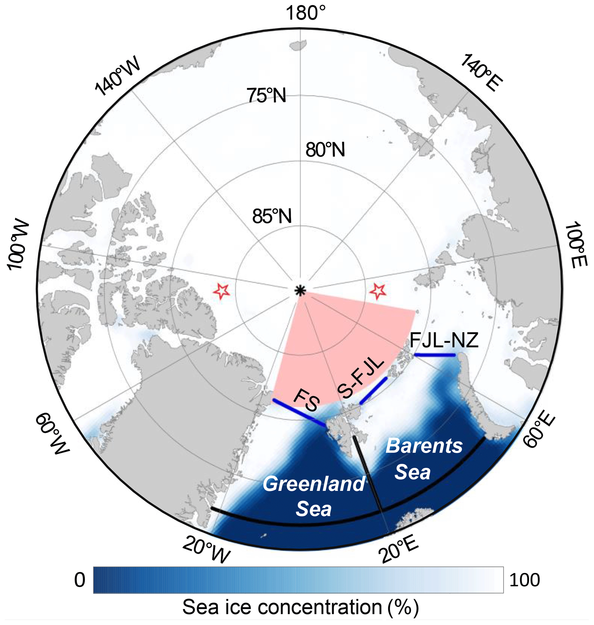
Figure 1Geographical locations of the Barents and Greenland seas. The three passageways defined for the calculations of sea ice area flux are indicated by blue lines. The Barents and Greenland seas are delimited by blue lines, black lines, and the coastline. The red stars indicate the locations (84∘ N, 90∘ W, and 84∘ N, 90∘ E) defined to calculate the central Arctic west–east air pressure gradient index (CAI). The Atlantic sector of the TPD from 15∘ W to 80∘ E is shaded in red. The background is the average sea ice concentration in January–March 2020.
2.2 Data
We used the National Snow and Ice Data Center (NSIDC) Polar Pathfinder version 4 sea ice motion (SIM) vectors and National Oceanic and Atmospheric Administration (NOAA)/NSIDC Climate Data Record passive microwave sea ice concentration (SIC) version 4 (Tschudi et al., 2019; Meier et al., 2021) to calculate the SIAF from the Arctic Ocean to the BGS in the study year and the climatological average in 1979–2020. The choice of this SIM product was motivated by its spatial completeness and temporal continuance. The SIM product is the most optimal merged interpolation result using satellite remote sensing data, buoy observations, and reanalyzed wind data (Tschudi et al., 2020). This product provides daily ice drift components georeferenced to the Equal-Area Scalable Earth Grid (EASE-Grid) with a spatial resolution of 25 km. The SIC product was a rule-based combination of SIC estimates from the National Aeronautics and Space Administration (NASA) Team (NT) algorithm (Cavalieri et al., 1984) and NASA Bootstrap (BT) algorithm (Comiso, 1986), derived from the Scanning Multichannel Microwave Radiometer (SMMR), Special Sensor Microwave Imager (SSM/I), and Special Sensor Microwave Imager/Sounder (SSMIS) radiometers. Daily SIC fields were gridded on a 25 km resolution polar stereographic grid. Both datasets are available from October 1978 to the present. However, there is a gap in the SIC dataset from 3 December 1987 through 12 January 1988. The sea ice area (SIA) was defined as the cumulative area of the waters covered by sea ice with the SIC above 15 %. For the study region, we used the SIC data since 1979 to estimate the SIA anomaly from January to June in the study year of 2020. In addition, we used buoy observation data from MOSAiC and the International Arctic Buoy Programme (IABP) to prove the effectiveness of the reconstructed results of the sea ice backward trajectories in the study year of 2020 and years with extreme atmospheric circulation patterns.
The sea ice thickness (SIT) data used to characterize the sea ice conditions in the region of the BGS were mainly derived from satellite remote sensing observations and were supplemented by the modeling product in early summer. The remotely sensed SIT data were created from the merged CryoSat-2 and Soil Moisture and Ocean Salinity (SMOS) observations, hereinafter referred to as CryoSat-2/SMOS (Ricker et al., 2017). The CryoSat-2/SMOS dataset makes full use of the detectability of SMOS for thin sea ice (<1.0 m) and the measurement capability of CryoSat-2 for thicker sea ice, which ensures obtaining a more comprehensive product of SIT. Weekly CryoSat-2/SMOS SIT data were available on a 25 km EASE-Grid during the freezing season of October to mid-April from 2010 to the present. During the ice melt season from May–June, we used the monthly SIT modeling product obtained from the Pan-Arctic Ice Ocean Modeling and Assimilation System (PIOMAS; Zhang and Rothrock, 2003). PIOMAS is a coupled ice–ocean model assimilation system that has been extensively validated and compared with satellite, submarine, airborne, and in situ observations and has proved it has good performance in sea ice thickness inversion (Zhang and Rothrock, 2003; Schweiger et al., 2011; Stroeve et al., 2014; Wang et al., 2016). The monthly PIOMAS SIT is gridded on a generalized orthogonal curvilinear coordinate system with an average resolution of 22 km. We regridded the monthly SIT data on the 25 km EASE-Grid and calculated the monthly average CryoSat-2/SMOS SIT data to maintain the spatial and temporal consistency of the two SIT datasets. To assess the data consistency of these two SIT datasets, we calculated the SIT anomalies from December to April using the PIOMAS SIT to compare it with the CryoSat-2/SMOS SIT. We found that the spatially averaged difference between the PIOMAS and CryoSat-2/SMOS SIT anomalies from December to April is about 0.09–0.20 m, which is about 6.0 %–13.3 % of the monthly magnitude. The statistical correlation between the spatially averaged SIT anomalies in December–April calculated using the two datasets in 2011–2020 is 0.95 (P<0.05). Thus, we considered the difference between the two datasets to be acceptable for calculating SIT anomalies, and PIOMAS can be used to supplement the SIT data for CryoSat-2/SMOS during the melt season (i.e., May–June), although their absolute values still have deviations that cannot be ignored. Therefore, we used the CryoSat-2/SMOS SIT from December to April and the PIOMAS SIT from May to June in 2011–2020 to estimate the anomaly in SIT during the study year of 2020.
We used sea surface temperature (SST) from 2011–2020 to characterize the anomalies in oceanic conditions over the BGS during the study year, as SST can be used as a proxy for the physical state over a basin scale (Siswanto, 2020). The SST data were obtained from the NOAA Daily Optimum Interpolation SST High Resolution dataset version 2, which assimilated buoy, ship-based, and satellite SST data (Huang et al., 2021). In the ice-covered regions, the proxy SST from SIC is intermixed with in situ and satellite SSTs. The proxy SST is obtained by a simple linear regression with SIC (Reynolds et al., 2007), and when the SIC is above 35 %, the proxy SST is defined as the freezing points of seawater, which in turn is defined using the climatological sea surface salinity (Banzon et al., 2020). This dataset is available on a regular grid of 0.25∘ × 0.25∘.
The fifth-generation reanalysis ERA5 datasets from European Centre for Medium-range Weather Forecasts (ECMWF) provide sea level pressure (SLP), 2 m air temperature, and 10 m surface wind, as well as atmospheric surface net heat fluxes of longwave radiation, shortwave radiation, sensible heat, and latent heat (Hersbach et al., 2020). These variables, with about 30 km horizontal and 1 h temporal resolutions, were used to identify anomalies in surface atmospheric conditions or forcing over the study region. ERA5 uses an advanced 4D-Var assimilation scheme, with improved performance over the Arctic compared to ERA-Interim (Graham et al., 2019). The hourly SLP data from ERA5 were used to calculate the monthly CAI, defined as the difference between SLPs at 84∘ N, 90∘ W, and 84∘ N, 90∘ E. We used the monthly AO and NAO indices provided by the NOAA Climate Prediction Center (CPC). The AO index was constructed by projecting a daily 1000 hPa height anomaly at the 20∘ N poles onto the AO loading pattern (Thompson and Wallace, 1998). The NAO index is defined as the SLP difference between the Azores High and the Icelandic Low (Hastenrath and Greischar, 2001).
2.3 Methods
The SIAF was defined as the magnitude of the SIA conveyed through a defined gate during a given period. In accordance with Kwok (2009), we estimated the monthly SIAF by accumulating the daily integral of the products between the gate-perpendicular component of the SIM and SIC along the defined passageways. Note that there is no SIM vector when the SIC is below 15 % (Tschudi et al., 2019). In this case, the SIAF is ignored. Positive values correspond to the SIAF towards the BGS, while negative values are the opposite. Prior to the estimation of SIAF, we interpolated the SIC into the SIM projection and retrieved the gate-perpendicular SIM components. According to the trapezoidal rule, the SIAF was estimated as follows:
where n is the number of points along the passageway, ui is the gate-perpendicular SIM component, Ci is the SIC at the ith grid cell, and Δx is the width of a grid cell (25 km).
The corresponding error in SIAF depends on the uncertainties in SIM and SIC products, the sampling number along the passageways, and the calculation period. For daily SIM vectors, the error was estimated to be about 4.1 km d−1 (Tschudi et al., 2019). Several assessments indicated an accuracy of about 5 % in the SIC (Peng et al., 2013). Assuming that these two sources of error are independent, the uncertainty (σf) in estimating SIAF across a 1 km wide gate was estimated at about 2.92, 3.80, and 2.68 km2 d−1 for the Fram Strait, S-FJL, and FJL-NZ, respectively. If we assume that the errors in the samples are additive, unbiased, uncorrelated, and normally distributed, the uncertainty in daily SIAF is (Kwok, 2009), where L is the length of the gate, and Ns is the number of independent samples across the gate. From January to June, the monthly average uncertainties in SIAF through three passageways were estimated to be approximately 1.81 × 10³ to 1.96 × 10³ km2, which were about 3.7 %–13.9 % of the monthly magnitude and therefore considered negligible. We described the SIAF anomalies relative to the 1988–2020 climatology because differences in satellite data sources could lead to relatively low SIM speeds derived from the SMMR 37 GHz data during 1979–1987 compared to those derived from daily SSM/I 85 GHz data, SSMIS 91 GHz data, and/or Advanced Microwave Scanning Radiometer for EOS (AMSR-E) 89 GHz observations in the later years (Kwok, 2009). To quantify the relative contributions of changes in SIM and SIC to the variability in SIAF on a seasonal scale, we also calculated the correlation between the sum of the monthly SIAF and the mean SIM speeds/SIC through the three passageways for winter (JFM) and spring (AMJ) in 1988–2020.
To identify the source area of sea ice and describe the relationship between the SIAF and the sea ice transport before reaching the defined passageway, we also reconstructed the sea ice backward drift trajectories from the defined passageways (Fram Strait, S-FJL, and FJL-NZ) over the three defined periods with the ice drifting from the north from 1 January and into the passageways by 30 April, 31 May, and 30 June, respectively. The adoption of three periods to restructure the ice backward drift trajectories is conducive to further distinguishing the difference between the anomalies over the winter or the period of winter through spring. In addition, the reconstructed backward trajectory of sea ice from the defined passageway can help to identify the source area of the ice reaching the passageways, thus revealing the relationship between the sea ice outflow and the sea ice conditions in the source area. The sea ice backward drift trajectories were reconstructed according to Lei et al. (2019), and the zonal (X) and meridional (Y) coordinates of the backward ice trajectories were calculated as follows:
where U(t) and V(t) are the ice motion components at the time t along the ice trajectories and δt is the calculation time step of 1 d. Thereby, the course of time corresponding to the sea ice backward drift trajectory is reversed from the defined date to 1 January.
In order to reveal the contribution of the surface heat budget to sea ice melting, we calculated the potential change in SIT (Δh) over the time of t caused by anomalies in atmospheric surface net heat fluxes over the BGS, according to Parkinson and Washington (1979):
where ρ is the density of sea ice (917 kg m−3); L is the latent heat of fusion for sea ice (333.4 kJ kg−1); δFLw↓, δFSw↓, δH↓, and δLE↓ represent the anomalies in atmospheric surface net fluxes of longwave radiation, shortwave radiation, sensible heat, and latent heat, respectively, with positive values denoting the downward heat flux. We note that Eq. (4) focuses on the atmosphere-to-ice heat fluxes but ignores the effects of ocean heat flux. Thus, it can only be used to assess the impact of the atmospheric anomaly on the local sea ice mass balance.
3.1 Anomalies in atmospheric circulation patterns
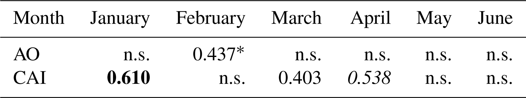
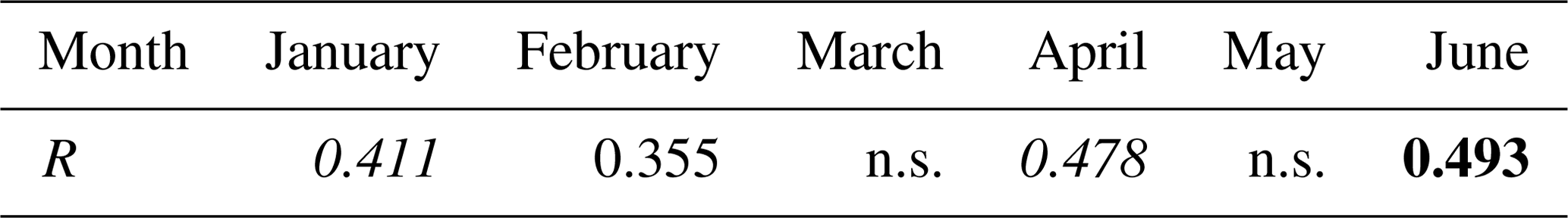
As shown in Table 1, the monthly AO was in an extremely positive phase from January to March 2020, with the values ranging in the top three among the years of 1979–2020. And then, the AO decreased to a smaller value in April and turned to a weakly negative phase in May–June 2020 (Fig. A1). The monthly CAI in January–June 2020 experienced a continuous positive phase with an average CAI of 8.5 hPa, which was the largest in 1979–2020. During winter–spring 2020, there were two peaks of the monthly CAI occurring in March and June, ranging in the first and fourth for 1979–2020, respectively.
In January–March 2020, accompanied by an unusual positive phase of the AO, the entire Arctic Ocean was almost dominated by abnormally low SLP compared to the 1979–2020 climatology (the first column of Fig. 2). In January 2020, a large-scale anomalously low SLP appeared near the Kara Sea, and the high-pressure center was observed in northern North America. This SLP pattern induced a positive CAI and northerly winds from the high Arctic towards the Barents Sea, accelerating the southward advection of Arctic sea ice into the Barents Sea and causing regional negative air temperature anomalies there (the second column of Fig. 2). In February 2020, the abnormally low SLP dominated near the Barents and Kara seas, inducing strong northerly winds in the Atlantic sector of the Arctic Ocean. This SLP and wind pattern continued to promote Arctic sea ice advecting into the BGS and keeping the negative air temperature anomalies in this region. In March 2020, the low SLP anomalies moved deeper into the central Arctic Ocean and induced westerly wind anomalies in the BGS.
In April 2020, the low SLP in the Arctic, centered in the northern Beaufort Sea, caused the sea ice to continue to advect towards the Barents Sea, and there were still small-scale negative air temperature anomalies over the Barents Sea (the third and fourth columns of Fig. 2). Subsequently, the SLP structure over the Arctic Ocean changed greatly in May 2020, with high-pressure anomalies observed in the Beaufort Sea. The air temperature turned into small positive anomalies over the Barents Sea in May–June 2020. The SLP structure in May 2020 was further conducive to Arctic sea ice advection towards northeastern Greenland. This large change in SLP structure led to the prominently enhanced positive CAI, which reached a second peak in June over 1979–2020; even the AO index decreased remarkably during this period (Table 1). Therefore, the AO mainly manifests the SLP structure of the pan-Arctic, regulating the sea ice outflow from the Arctic Ocean to the BGS by changing the axis alignment of the TPD, while the CAI mainly affects the wind forcing and ice speed in the TPD region, especially for the Atlantic sector.
Table 1The monthly AO index and CAI in winter–spring 2020 and their ranking in 1979–2020.
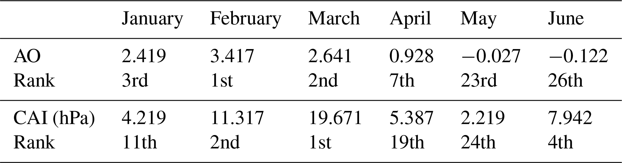
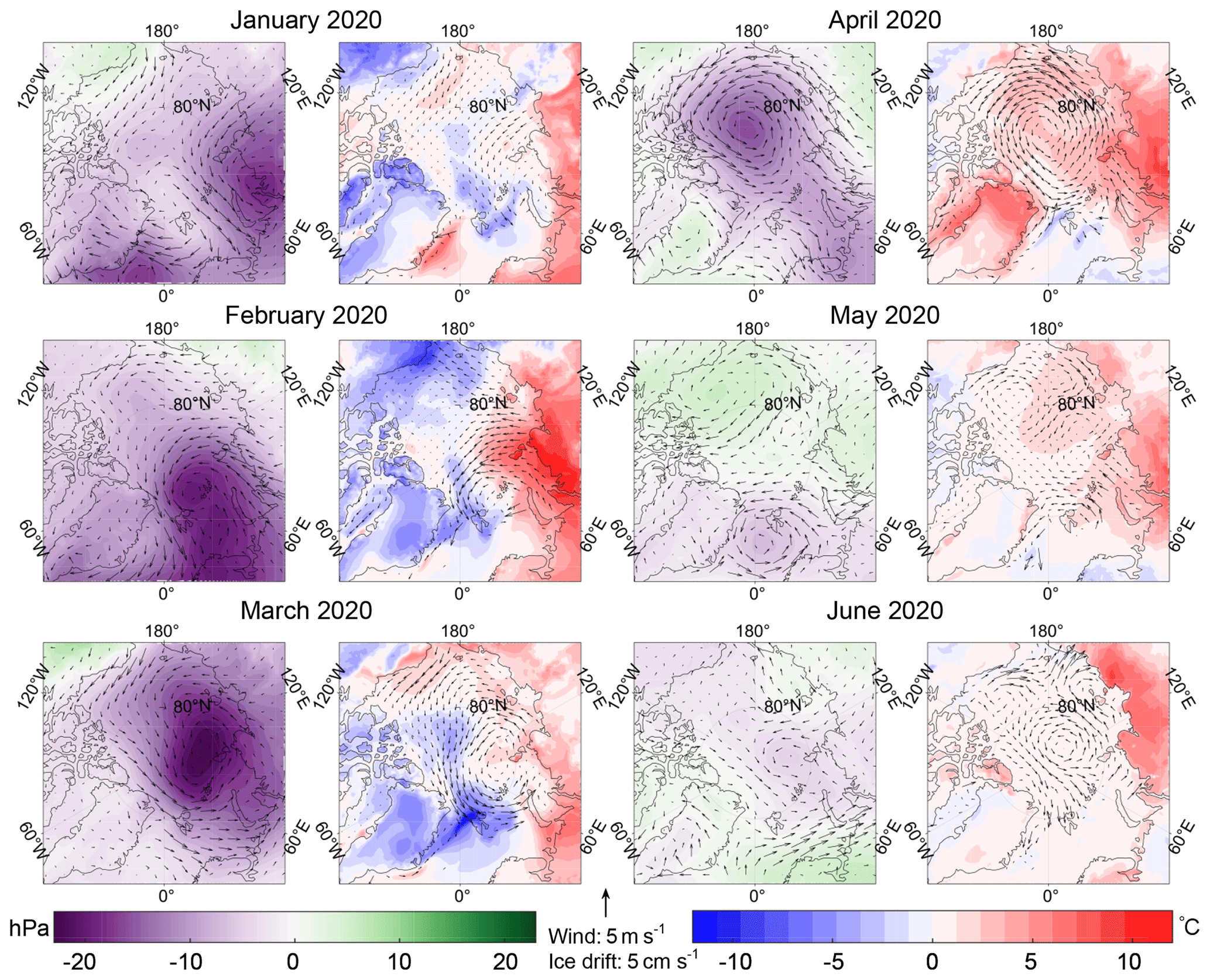
Figure 2Monthly mean SLP (shading) and 10 m surface wind (arrows) anomalies (the first and third columns) and 2 m air temperature (shading) and sea ice drift speed (arrows) anomalies (the second and fourth columns), during January–June 2020 relative to the 1979–2020 climatology.
3.2 Anomalies in Arctic sea ice outflow and its link to atmospheric circulation patterns
The extremely positive AO in winter (JFM) 2020 induced relatively high wind speeds over the Atlantic sector of the Arctic Ocean (the first column of Fig. 2), which led to the high SIM speeds along the TPD. Significant positive correlations between the monthly SIM speeds and the wind speeds in the Atlantic sector of the TPD have been identified in January–February, April, and June, as shown in Table A1. The 1988–2020 data revealed that the SIM speeds perpendicular to the passageways are significantly correlated with the accumulated SIAF through three passageways in both winter and spring ( and +0.85, respectively; P<0.001), while the corresponding correlation between SIC and the SIAF is only significant in winter (, P<0.05). In January–June 2020, SIC anomalies contributed 3.9 % to SIAF anomalies and SIM speed anomalies contributed 71.7 %. The anomalies of Arctic sea ice outflow through our defined passageways were mainly dominated by SIM anomalies in winter–spring 2020. Compared to the 1988–2020 climatology, the accumulated SIAF values across three passageways were all at the above-average level in January–March and June, with the largest positive anomalies occurring in March 2020.
In winter 2020, the cumulative SIAF through the Fram Strait was 1.19 × 10⁵ km2, which was larger than the 1988–2020 average by about 20 % and was the second largest in 2010–2020. Especially in March 2020, the monthly SIAF through the Fram Strait (5.77 × 10⁴ km2) was the second largest in 1988–2020. The winter cumulative SIAF through S-FJL in 2020 (1.51 × 10⁴ km2) was also the second largest in 2010–2020. However, the winter cumulative SIAF through the FJL-NZ in 2020 (2.76 × 10⁴ km2) was only about 81.0 % of the 1988–2020 average. That is, the extremely positive AO in winter 2020 only significantly facilitated more sea ice outflow through the Fram Strait and S-FJL, while sea ice outflow through the FJL-NZ did not respond significantly to the extremely positive AO. Under the influence of a positive CAI in spring (AMJ) 2020, the cumulative SIAF through the Fram Strait was still at an above-average level, while the spring cumulative SIAF through the S-FJL and FJL-NZ in 2020 was only 67.5 % and 14.1 % of the 1988–2020 average, respectively. Such low SIAF through the FJL-NZ passageway may be related to the enhanced inflow from the Barents Sea into the Arctic Ocean through this passageway (Polyakov et al., 2023). This implies that the SIAF through these two passageways, especially for the FJL-NZ passageway in the east, was not facilitated by a positive CAI in spring 2020.
Overall, the total SIAF anomalies in January–June 2020 were most pronounced in the Fram Strait, followed by those observed in the S-FJL passageway, with positive anomalies of 2.35 × 10⁴ and 1.40 × 10⁴ km2 (Fig. 3), respectively. However, negative anomalies were observed in the FJL-NZ passageway. This indicates that only the SIAF through the Fram Strait and S-FJL responds to both the extremely positive phase of the winter AO and the continuous positive phase of the winter–spring CAI. Furthermore, the values of the total SIAF anomalies in January–June 2020 through these three passageways were not prominent in 1988–2020 (last row of each panel in Fig. 3). This implies such discontinuous extreme AO and CAI values only had a moderate impact on the Arctic sea ice outflow through these three passageways, especially the FJL-NZ in the east.
We further quantified the relationship between SIAF and two atmospheric circulation indices (AO and CAI) from 1988 to 2020 to test the robustness of the influencing mechanism identified in 2020. Here, we chose the Fram Strait as the investigated passageway because, in winter–spring 2020, the Fram Strait contributed the most (77.6 %) to the total SIAF through the three passageways. We calculated the correlation coefficient (R) between the detrended monthly SIAF and the detrended AO and CAI from January to June for the period 1988–2020 (Table 2). During January–June, there was a significant positive correlation between SIAF and the AO identified in February but not in other months. This is consistent with a weak linkage between the AO and SIAF through the Fram Strait in 1979–2014 (Polyakov et al., 2023). There was also a significant positive correlation between the monthly SIAF and CAI in January, March, and April (R=0.61, 0.40, and 0.54, respectively; P<0.05), which suggests that the relatively high CAI could induce a southward advection of Arctic sea ice to the BGS, especially during the period (March–April) with a relatively high ice motion speed in the regions north of the BGS compared to other months (e.g., Lei et al., 2016).
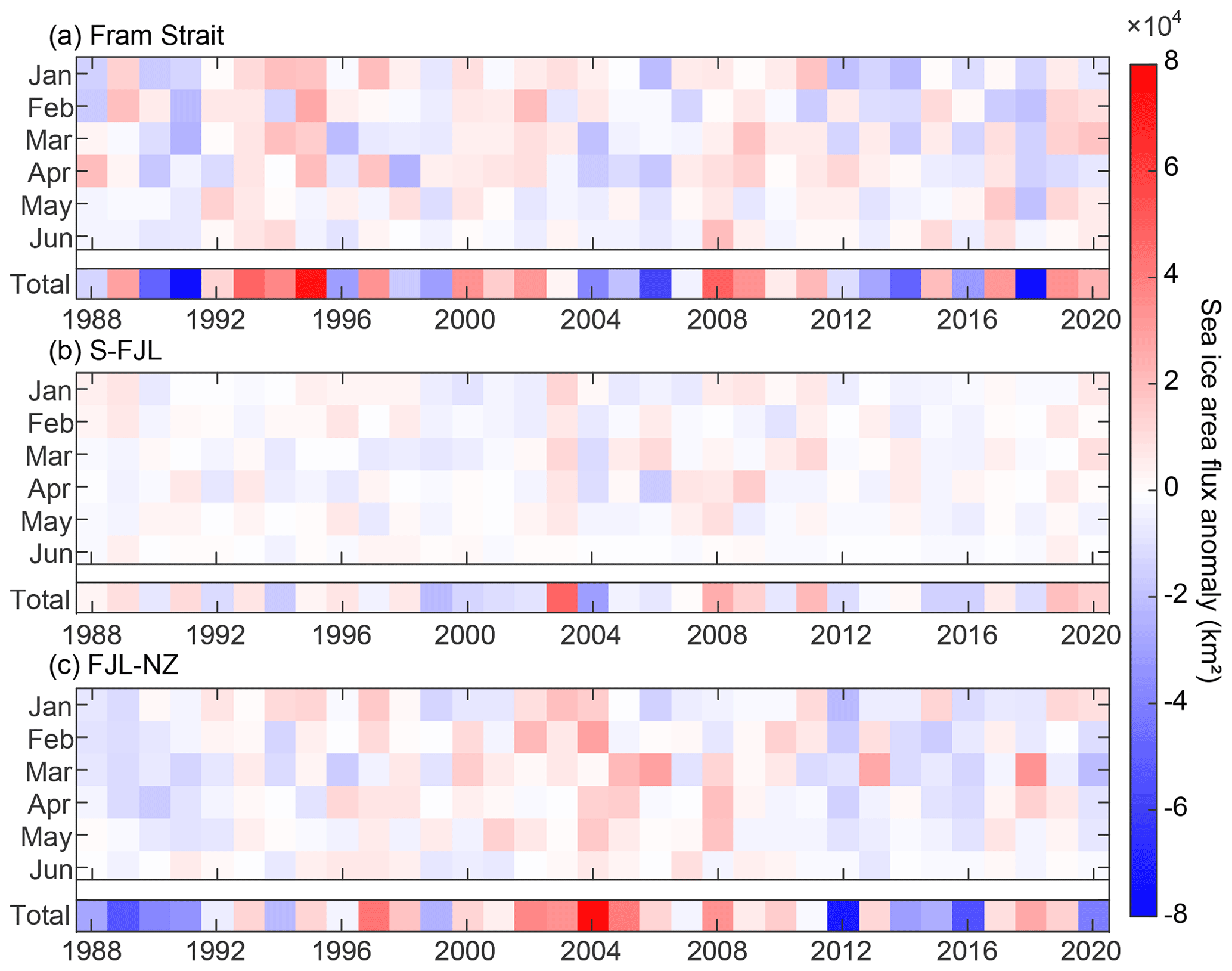
Figure 3Monthly anomalies of sea ice area flux (SIAF) through the Fram Strait, S-FJL, and FJL-NZ from 1988 to 2020. The last row of each panel represents the anomalies of cumulative SIAF from January to June.
Table 2Correlation coefficient (R) between monthly sea ice area flux (SIAF) through the Fram Strait and atmospheric circulation indices in 1988–2020.
* Significance levels are P<0.001 (bold), P<0.01 (italic), and P<0.05 (plain); n.s. denotes insignificant at the 0.05 level.
3.3 Anomalies in sea ice backward trajectories from the passageways
The sea ice backward trajectories can be traced back to the source region of sea ice that advected to the passageways. The broader distribution of the original sea ice area implies that more ice would enter the passageways, leading to an increased sea ice outflow. The reconstructed sea ice backward trajectory in January–June 2020 was similar to that of the MOSAiC ice station (Nicolaus et al., 2021) in the same period, with almost parallel orientation and a very close drift distance between them (Fig. 4c). The slight dislocation was mainly attributed to the inconsistent termination location between the reconstructed backward trajectory and the MOSAiC trajectory on 30 June 2020. Using the endpoints of the two buoys obtained from MOSAiC as the start points of the reconstructed backward trajectories, the Euclidean distance between the termination locations of the reconstructed backward trajectory and the starting locations of the buoy trajectories is averaged out at 63 km, and their trajectories almost overlapped, with the cosine similarity between them reaching 0.85. We also compared the consistency between the reconstructed backward trajectories and the buoys' trajectories, with the data obtained from the International Arctic Buoy Programme, when the extreme positive or negative (±1 standard deviation) phase of the AO and CAI occurred (hereinafter referred to as AO+, AO−, CAI+, and CAI−). As shown in Table A2, in the AO+ and CAI+ cases, the average Euclidean distances between the reconstructed backward trajectories and buoy trajectories were smaller than in the AO− and CAI− cases. This indicates that the sea ice drift distances obtained from the reconstructed backward trajectories are closer to the buoy observations in the AO+ and CAI+ cases than in the AO− and CAI− cases because the tortuous sea ice trajectories were relatively large under the AO− and CAI− compared to under the AO+ and CAI+. However, the cosine similarities were above 0.9 in all AO and CAI cases. This suggests that the orientation of the reconstructed backward trajectories is reliable regardless of the phases of the AO and CAI. It increases our confidence in using this method to reconstruct the ice backward trajectories to identify the source region of sea ice.
Compared to the sea ice backward trajectories reconstructed using the average SIM vector of 1988–2020 (Fig. 4d–f), the sea ice backward trajectories from the Fram Strait in 2020 tended westwards (Fig. 4a–c). This implies that the orientation of the TPD was more favorable for exporting thicker ice from the western Arctic Ocean and northern Greenland to the Fram Strait during winter–spring 2020. For the Fram Strait, the terminations of the sea ice backward trajectories in 2020 were concentrated at 87–90∘ N, which indicates that most of the sea ice advected into this passageway was from the region close to the North Pole. In all three investigation periods, the net distances from the start points at the defined passageways to the terminations of the reconstructed ice backward trajectories in 2020 were the second longest in 1988–2020. In S-FJL, sea ice was mainly advected from the confluence of the Kara Sea and the central Arctic Ocean (Fig. 4), and its backward trajectories were more curved than those from the Fram Strait. Furthermore, no reasonable backward trajectories of sea ice could be acquired for the S-FJL passageway according to the starting points of 31 May and 30 June. This was because the relatively low SIC in this region by late spring had restricted the acquisition of valid SIM data. The sea ice advected through the FJL-NZ passageway was mainly from the Kara Sea. Thus, the identification of the source areas of sea ice that reached the passageways can explain why the changes in SIAF through the S-FJL and FJL-NZ passageways are not as sensitive to changes in the CAI pattern as those through the Fram Strait.
Overall, compared to the 1988–2020 averages, the sea ice backward trajectories through the Fram Strait in winter–spring 2020 were characterized as longer and farther west. Particularly, the net distances between the terminal points on 1 January and the starting points from the Fram Strait on or after 30 April, 31 May, and 30 June of each year in 1988–2020 were significantly positively correlated with the corresponding SIAF (, +0.72, +0.75, respectively; P<0.001). Thus, the enhanced sea ice motion along the TPD during January–June 2020 promoted more Arctic sea ice export towards the BGS, which in turn accelerated the reduction in sea ice over the pan-Arctic Ocean.
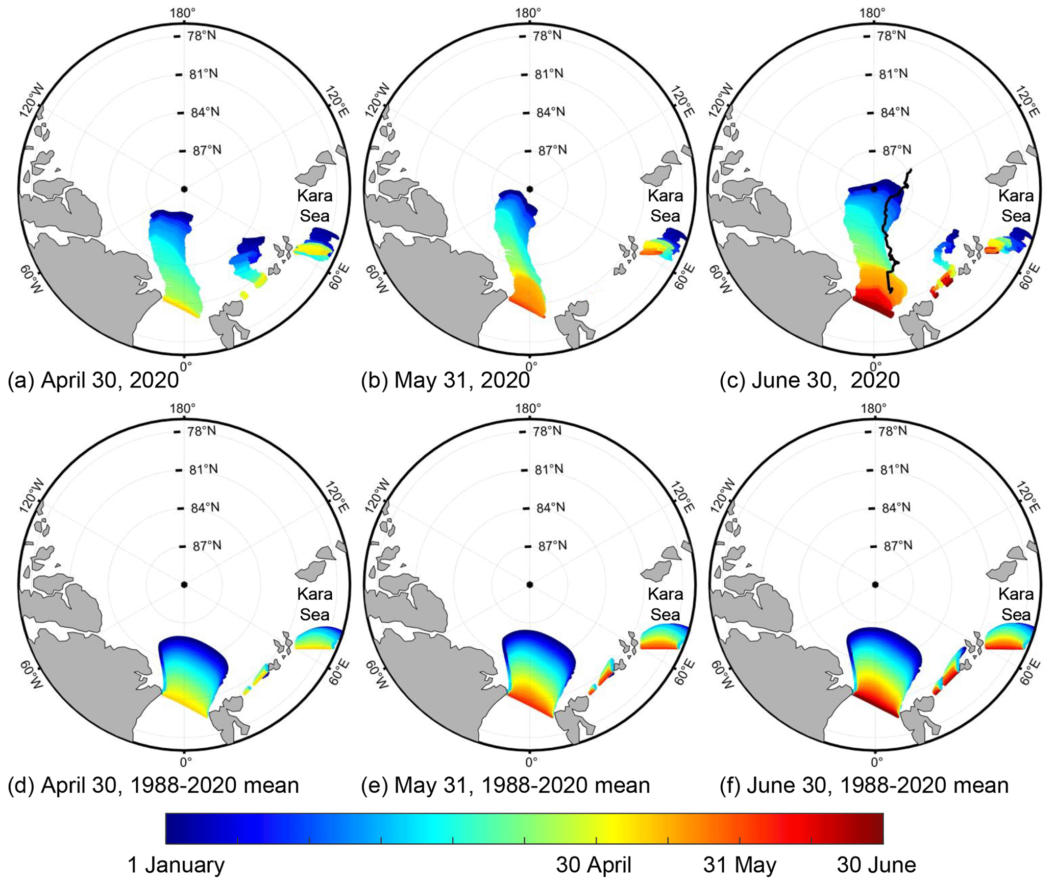
Figure 4Backward trajectories of sea ice advected to the Fram Strait, S-FJL, and FJL-NZ passageways. Panels (a)–(c) show the backward trajectories of sea ice arriving at the passageways by 30 April, 31 May, and 30 June 2020, respectively. Panels (d)–(f) are the same as (a)–(c) but estimated using the average sea ice motion vector from 1988 to 2020. All termination data of the reconstructed backward trajectories were set to 1 January. The black line in panel (c) represents the MOSAiC trajectories from 1 January to 30 June 2020.
3.4 Anomalies in sea ice and sea surface temperature in the Barents and Greenland seas
SIA in the BGS generally reaches its annual maximum in April each year and then begins to decline as the air and ocean temperatures rise. In April–June 2020, the SIA in the BGS reached the first, second, and fourth largest in 2010–2020. It was much higher compared to the value obtained from the linear decreasing trend from 1979 to 2020, indicating that the SIA in the study year was higher than the expectation. In the Barents Sea, the monthly SIA values for January–April 2020 all ranged in the top three for 2010–2020 (Fig. 5a). The SIA in the Greenland Sea was similar to that in the Barents Sea, with monthly SIA values in April–June 2020 ranking the first or second largest in 2010–2020. Such a large SIA in the BGS during spring 2020 was linked to a more massive sea ice export from the central Arctic Ocean because we found a significant correlation (, P<0.05) between the total SIAF anomalies through the three defined passageways and the SIA in the BGS based on the 1988–2020 data.
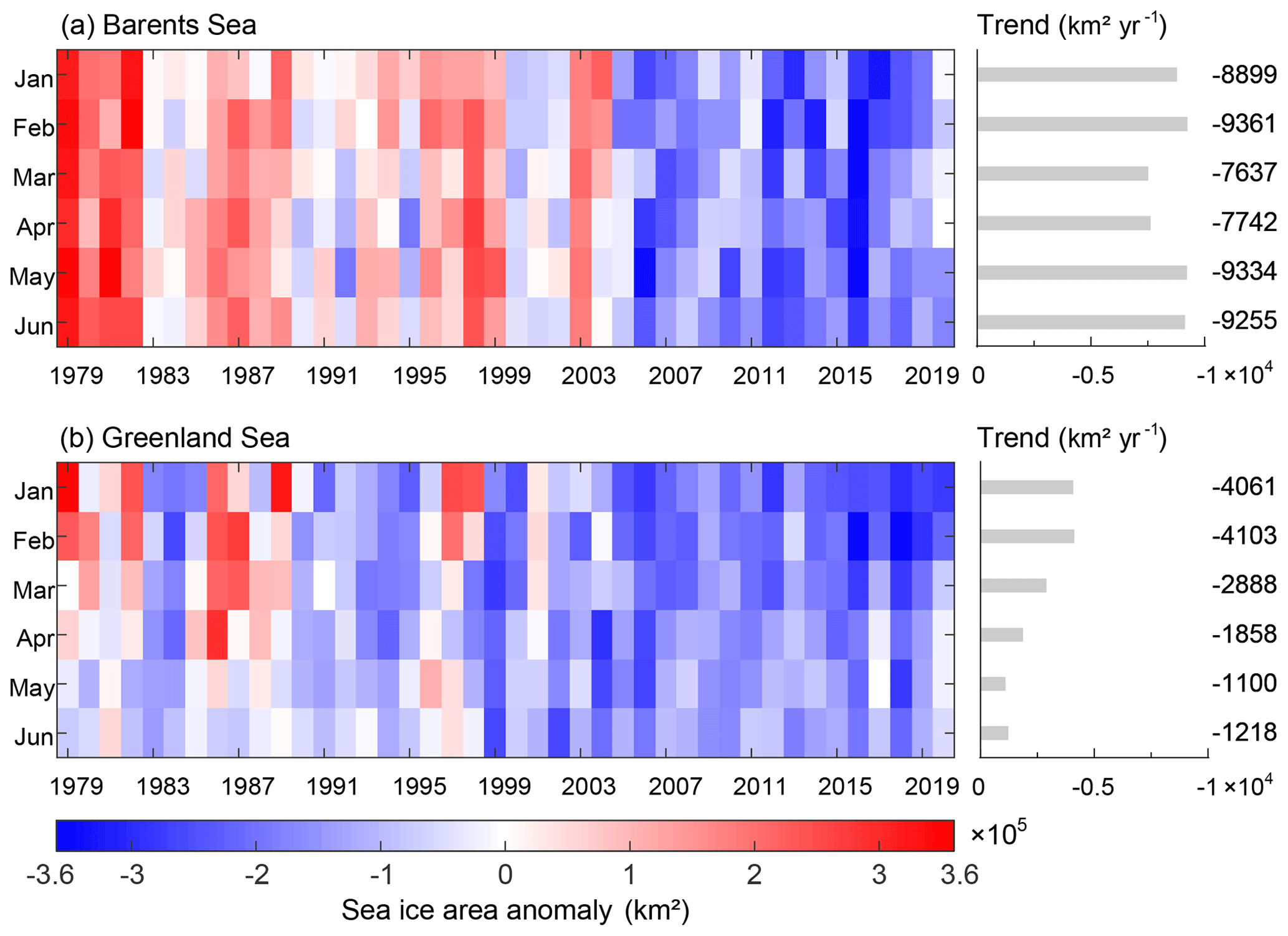
Figure 5Monthly sea ice area (SIA) anomalies in the Barents and Greenland seas from 1979 to 2020. Also shown on the right are the corresponding long-term linear trends, which are all statistically significant at the 0.05 level.
As shown in Fig. 6, negative SIT anomalies, i.e., ice thinner than the average, were observed mainly in the Greenland Sea during December 2019. The SIT anomalies were relatively small in the Barents Sea. Since January 2020, more pronounced positive SIT anomalies, i.e., ice thicker than the average, were observed in the Barents Sea and persisted to June. In the Greenland Sea, the positive SIT anomalies gradually increased, particularly on the eastern side from March 2020 and were especially widespread in May–June, while the negative SIT anomalies were mainly observed on the western side. This east–west pattern of SIT anomalies could be attributed to the increased outflow of thicker sea ice from the central Arctic through the Fram Strait.
Furthermore, widespread negative anomalies of SST (−1 to −3 ∘C, Fig. 7) were observed in the BGS in April–June 2020, with monthly SSTs being the lowest for 2011–2020. In addition, the negative SST anomalies over the Greenland Sea persisted until July 2020. The detrended correlations between the monthly SIA and contemporaneous SST in the BGS from April to June over 1982–2020 (Table A3) were significantly negative. Thus, the abnormally large Arctic sea ice outflow in winter–spring 2020 led to an increased SIA and the associated relatively high albedo in the BGS, thereby preventing the absorption of solar radiation by the ocean and suppressing the rise in SST. In turn, relatively cold seawater was not conducive to sea ice melting there. The corresponding correlation coefficients in the Greenland Sea were weaker compared to those in the Barents Sea, which may be due to the relatively complex influencing factors in the SST variations in the Greenland Sea. That is to say, the northwestern Greenland Sea is protected from cooling effects due to sea ice and surface current outflow from the north, while the southeastern part is subject to warming effects from warm Atlantic waters (Wang et al., 2019). Regionally, we found that the negative correlation coefficients between SIA and SST are more significant in the southern BGS (72–76∘ N) than in the northern part (76–80∘ N). This is likely because the SST is more closely correlated with the SIC in areas with less sea ice (Wang et al., 2019). In addition, we examined the statistical relationship between the detrended April SIA and the detrended monthly SST with a lag of 1–3 months in the BGS (Table A4). In the Barents Sea, the April SIA still had a significant negative effect on the increase in SST until July, i.e., with a lag of 3 months, whereas in the Greenland Sea, the significant influence of April SIA on the SST only lasted until June. This difference suggests that the sea ice anomalies in the Barents Sea have a longer memory for the impact on the SST than those in the Greenland Sea.
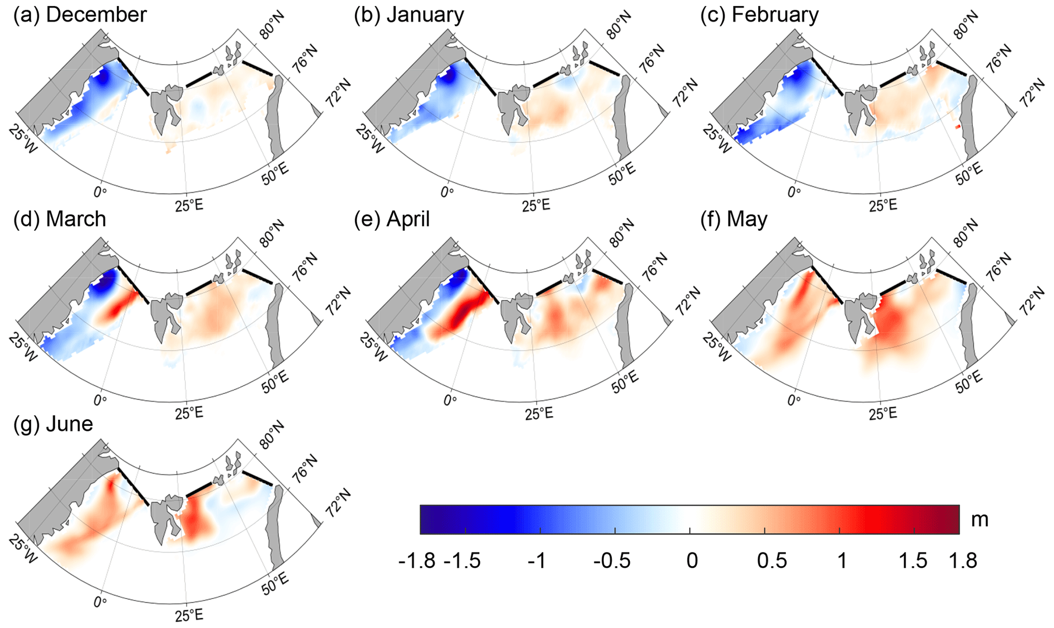
Figure 6Sea ice thickness (SIT) anomalies in the Barents and Greenland seas from December 2019 to June 2020 compared to the 2011–2020 average obtained from the CryoSat-2/SMOS product (December–April) and PIOMAS modeled data (May–June).
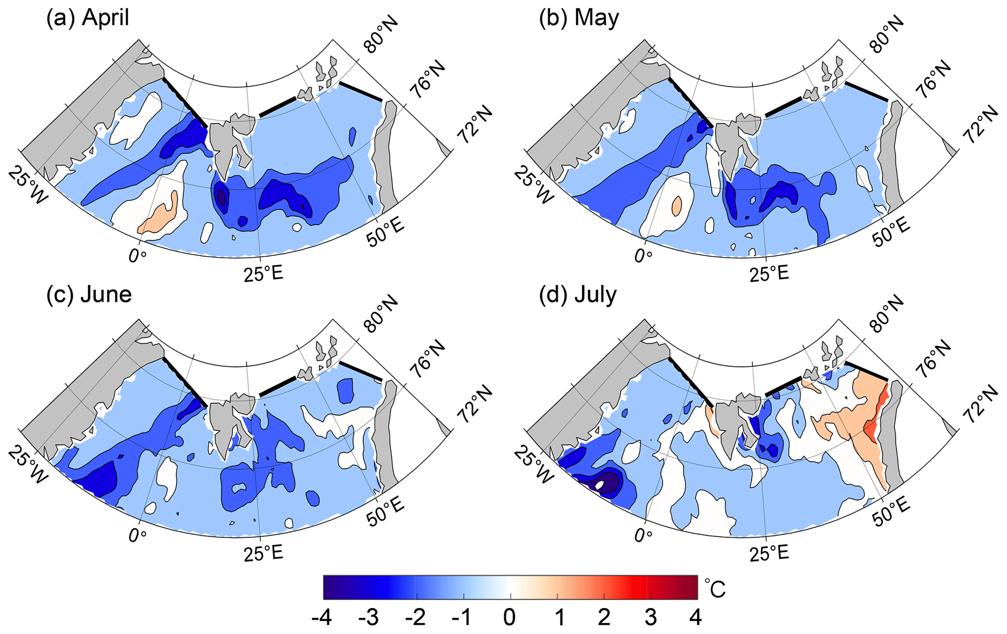
Figure 7Monthly sea surface temperature (SST) anomalies in the Barents and Greenland seas from April to July 2020 compared to the 2011–2020 average.
4.1 Impact of extreme atmospheric circulation patterns on sea ice processes before they reach the Fram Strait
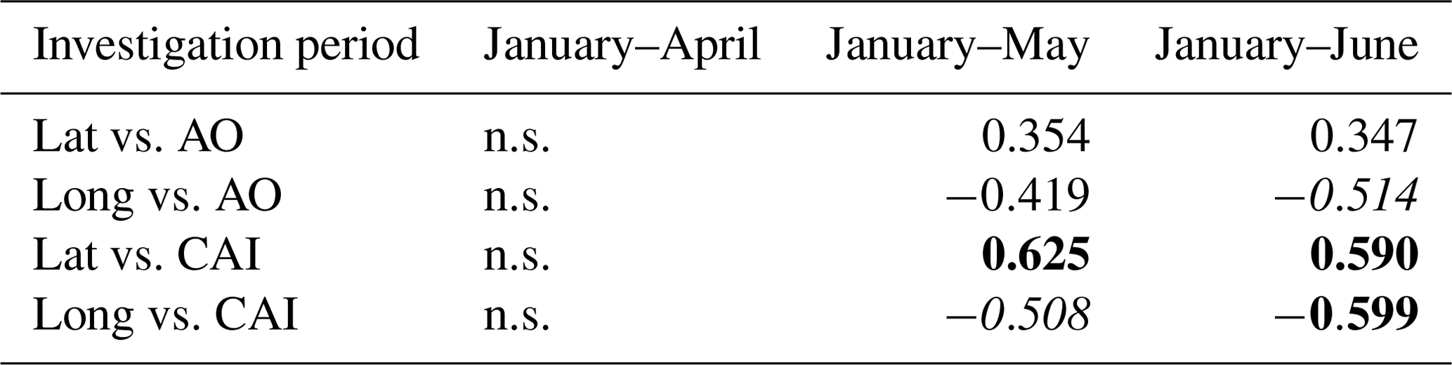
To explore the changes in sea ice backward trajectories in response to extreme atmospheric circulation patterns, we examined the years in which the AO+, AO−, CAI+, and CAI− occurred in winter, based on which we obtained the mean SIM field and reconstructed the January–June sea ice backward drift trajectories arriving in the Fram Strait in June of the corresponding years (Fig. A2). In the AO+ case, the end of sea ice backward trajectories (blue trajectory in Fig. A2a) extended westwards, which indicated that the TPD originated further west. This suggests that the winter AO+ is more conducive to sea ice outflow from the central Arctic Ocean to the BGS (e.g., Rigor et al., 2002). Thus, we believe the relationship between the positive phase anomalies of the AO and the westward alignment of the TPD identified in 2020, as shown in Fig. 4, is robust, whereas in the AO− case, the sea ice backward trajectories were closer to the prime meridian and relatively eastwards compared to the AO+ case. Under the influence of the AO−, the expanding Beaufort Gyre can weaken the strength of the TPD and reduces Arctic sea ice export (e.g., Zhang et al., 2022). Associated with either the CAI+ or the CAI−, the sea ice backward trajectories were similar to those under the corresponding phase of the AO. However, in the two investigated periods of January–May and January–June, there is a higher positive (negative) correlation between the latitude (longitude) of sea ice backward trajectory endpoints and the CAI compared to the AO (Table A5). This relationship was due to the fact that the CAI+ might directly enhance the TPD by strengthening the straightforward wind forcing, hence favoring sea ice outflow from the central Arctic Ocean into the Fram Strait. However, an insignificant correlation between them was obtained in the investigated period of January–April. This is likely related to the fact that the sea ice backward trajectories reconstructed in this period were relatively short and the variations in the backward trajectory endpoints between the years were relatively small.
The January–June average sea ice backward trajectories in the AO+, AO−, CAI+, and CAI− cases were then used to further check whether extreme atmospheric circulation patterns have influences on the atmospheric forcing of sea ice thermodynamic processes. We obtained the freezing degree days (FDD), which are the temporal integral of air temperature below the freezing point over the freezing season. The results showed that, only the FDD in the AO+ case (2616 K d−1) were lower than the 1988–2020 mean (2695 K d−1). This implies that the endpoint of the backward trajectory corresponding to the AO+ would be further south and east (Fig. A2); the near-surface air temperature over there would be significantly higher than that in the northwest, which is unfavorable for sea ice growth. We also compared the lengths of time that the sea ice backward trajectory was within the region south of 82∘ N before the floe reached the Fram Strait, as sea ice there was affected by strong heat supply from the ocean (Sumata et al., 2022). In the AO+ (CAI−) case, the residence time in the region south of 82∘ N before ice reached the Fram Strait was 54 (57) d, which is longer than in the AO− (CAI+) case (43 (38) d). This suggests that sea ice in the AO+ or CAI− cases was exposed to strong heat from the ocean for a longer period and therefore facilitated larger sea ice melt than in the AO− or CAI+ cases.
4.2 Other factors affecting sea ice anomalies in the Barents and Greenland seas
The impact of Arctic sea ice outflow on the SIA in the BGS would be weakened by both local atmospheric and oceanic forcing (Frey et al., 2015; Lind et al., 2018). Here, we focus on the effect of atmospheric anomalies on sea ice conditions. The persistence of negative air temperature anomalies in the BGS from February to April 2020 (the second and fourth columns of Fig. 2), roughly 2 to 6 ∘C lower than the 1979–2020 climatology, would restrict the sea ice melting there. Especially in March 2020, negative air temperature anomalies covered almost the entire BGS, and the region with the −6 ∘C anomalies occurred in the coincident region with positive monthly SIT anomalies (Figs. 2 and 6). Moreover, compared to the 1979–2020 climatology, the monthly atmospheric surface heat fluxes showed positive (upward) anomalies over the climatological ice-covered BGS (regions with the SIC above 85 % for the 1979–2020 climatology) in January–March 2020 (Fig. 8), which were mainly dominated by turbulent heat flux (35.7–38.6 W m−2), accounting for 84.2 %–98.9 % of the atmospheric surface heat flux anomalies. Especially in February and March 2020, the upward anomalies in sensible heat flux were 1.7–2.4 times the latent heat flux. This was likely due to the relatively large air–sea temperature difference and relatively high wind speeds in the BGS during this period, which would have resulted in an unstable atmospheric boundary layer and the increased atmospheric heat flux from the ocean to the air (Minnett and Key, 2007). In addition to turbulent heat flux, the net longwave radiation revealed relatively small upward anomalies (0.4–8.9 W m−2) persisting from January to April 2020, which were also favorable for preventing ocean warming and ice melting. From April to June 2020, the direction of monthly anomalies in atmospheric surface heat fluxes shifted from upwards to downwards, but the values are smaller relative to the values in January–March. It is worth noting that upward anomalies in net shortwave radiation were observed in June 2020 over the study region, which coincided with the relatively large SIA and the associated relatively high regional albedo. Over the climatological ice-covered BGS, anomalies in the cumulative monthly atmospheric surface heat flux from January to April 2020 were associated with a reduced decrease of 0.12–0.51 m in SIT, estimated using Eq. (4). This was conducive to the survival of sea ice during spring and early summer 2020.
The NAO did not exhibit an extreme positive phase in 2020. However, we still investigated the relationship between the NAO index and the sea ice conditions in the BGS, considering the regional influence of the NAO on the BGS. In 2020, the NAO index remained positive from January to March, similarly to the positive AO index. It favored Arctic sea ice outflow to the BGS to some extent, as a significant positive correlation (R=0.36, P<0.05) between the NAO index and the SIA in the southern BGS was identified in January. The positive phases of NAO in January–March also induced a stronger northerly wind over the North Atlantic, carrying cold air southwards and thus decreasing the air temperature in the BGS (e.g., Hurrell, 2015), as shown in the second column of Fig. 2, which was not conducive to sea ice melting. Thus, the NAO mainly regulates the wind forcing of the BGS, rather than the atmospheric forcing, before sea ice reaches our defined passageways, as the AO and CAI do.
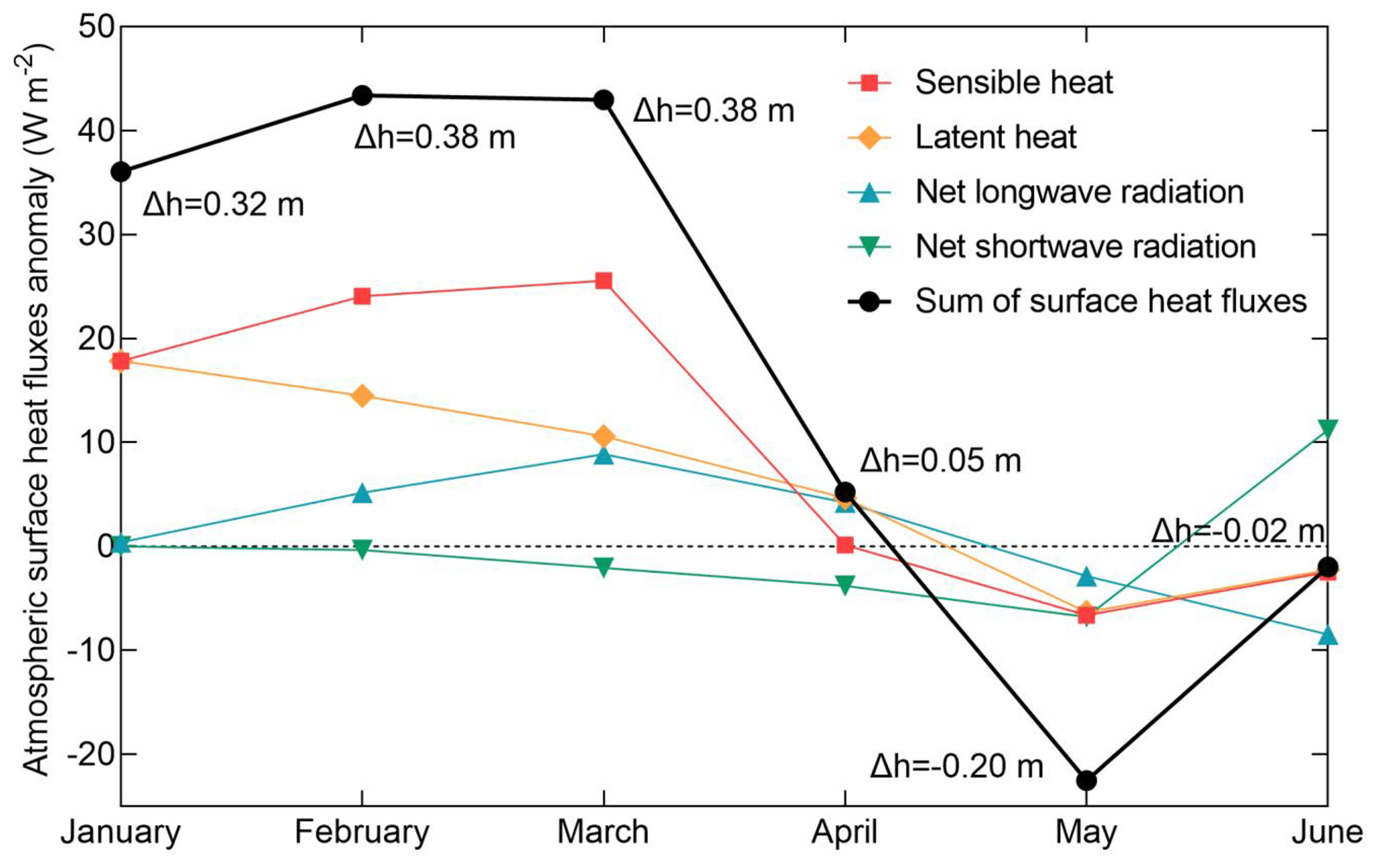
Figure 8Monthly anomalies in atmospheric surface heat fluxes of sensible heat, latent heat, net longwave radiation, and net shortwave radiation averaged over the climatological ice-covered region of the BGS from January to June 2020 compared to the 1979–2020 average, with positive values denoting the upward fluxes. Δh refers to the changes in SIT estimated from Eq. (4) based on the sum of atmospheric surface heat flux anomalies of the corresponding month.
4.3 Are the anomalies and their connections identified in winter–spring 2020 typical in climatology?
In the past decade, positive anomalies in the winter–spring SIAF through our defined passageways relative to the 1988–2020 climatology were also identified in 2011, 2017, and 2019, close to the value in 2020 (Fig. 3). Therefore, we also quantified the anomalies of sea ice and ocean conditions in the BGS for these years to assess the robustness of the seasonal feedback mechanisms identified in winter–spring 2020. During these 3 years, the sea ice backward trajectories reconstructed starting 30 April, 31 May, and 30 June were also characterized as longer and farther west compared to the 1988–2020 climatology. This suggests that the ice speeds along the TPD were relatively large and could partially contribute to the positive SIAF anomalies in these years. In the BGS, although small negative SIA anomalies were observed in March–June 2011, 2017, and 2019 compared to the 1979–2020 climatology, their values were still much higher than those estimated from the long-term linear decreasing trends since 1979 by 0.16 × 104–2.95 × 10⁴, 0.33 × 10⁵–1.41 × 10⁵, and 0.71 × 10⁵–1.09 × 10⁵ km2, respectively. During these 3 years, similar upward anomalies in accumulated net atmospheric surface heat fluxes were also identified in January–March, suggesting the potential coupling mechanism between sea ice coverage and the surface heat budget in the BGS. However, compared to the 1979–2020 climatology, there were positive air temperature anomalies in January–March 2011, 2017, and 2019, in contrast to the negative air temperature anomalies in 2020. This may subsequently contribute to the relatively small negative SIA anomalies in these years compared to in 2020. The SIT anomalies were calculated only for 2017 and 2019 since satellite SIT data were not available prior to 2011, and we found that the BGS also showed small positive anomalies from March to June for both years compared to the average since 2011. Furthermore, the sea ice anomalies in these years also had impacts on the oceanic conditions of the BGS in the subsequent April–June. The monthly SSTs in May–June of 2011, 2017, and 2019 all ranked the second to fourth lowest for 2010–2020.
For comparison purposes, the extremely negative SIAF anomalies through the defined passageways in winter–spring should also be taken into consideration; we thus chose the year of 2018 as the case of low Arctic sea ice outflow (Fig. 3). In 2018, the sea ice backward trajectories were all shorter than for the 1988–2020 climatology over all the periods of January–April, January–May, and January–June. This suggested that the southward SIM speeds along the Fram Strait were relatively low from January to June in 2018 (Sumata et al., 2022). In the BGS, the SIA in May–June 2018 was lower by 4.44 × 10⁴ and 3.63 × 10⁴ km2 compared to the SIA estimated from the long-term linear decreasing trends since 1979. In January–June 2018, there were widely negative SIT anomalies in the BGS compared to the 2011–2018 climatological mean, which is consistent with the abnormal SIT reduction in the Fram Strait region confirmed by Sumata et al. (2022). The oceanic conditions in the BGS were also affected. In May, the mean SST in 2018 was higher than that in the high-outflow cases (2011, 2017, and 2019) by 20 %–40 %, consistent with the negative correlation between SIA and SST (Table A3).
We also assessed the impact of the positive AO in summer (JAS) on the BGS, since sea ice motion generally responds more strongly to the atmosphere in summer. Using the year of 2016 in which the AO+ occurred in summer, we found that the SIAF through the Fram Strait in this summer was much larger than the 1988–2020 climatology, ranking the third and fourth for 1988–2020. This suggests that the AO+ also contributes to the enhanced Arctic sea ice outflow to some extent in summer. However, due to local processes, the SIA of the BGS in this summer was even smaller than that estimated from the linear regression of 1979–2020.
Note that we also expect that the influences of abnormally high Arctic sea ice outflow on the sea ice and other marine conditions in the BGS will gradually weaken if the Arctic sea ice continues to thin and the northward Atlantic Ocean heat flow continues to increase because the thinner ice under the increased oceanic heat would not be conducive to the survival of sea ice in the BGS.
In this study, we investigated the impacts of atmospheric circulation anomalies on Arctic sea ice outflow in the winter and spring of 2020, assessed anomalies in sea ice and oceanic conditions in the TPD downstream region of the BGS and the linkages between them, and then discussed the factors contributing to the sea ice anomalies in the BGS.
Compared to the 1979–2020 climatology, the AO experienced an unusually large positive phase in January–March 2020. In the context of this, the SLP structure, associated with the positive CAI, induced strong northerly winds along the Atlantic section of the TPD, leading to enhanced SIM speeds, which then facilitated Arctic sea ice outflow to the BGS. The variabilities in seasonal accumulated SIAF in 1988–2020 through these passageways were mainly dominated by the change in SIM speed ( for January–June; P<0.001), which was more significant than that related to the changes in SIC ( for January–March; P<0.05). In the following 3 months, the AO decayed to be negative, while the CAI remained positive, which ensured a continuous enhanced Arctic sea ice outflow to the BGS. Therefore, in January–March and June 2020, the total SIAF through three passageways north of the BGS was relatively large compared to the 1988–2020 climatology, mainly through the Fram Strait. The SIAF through the Fram Strait was significantly positively correlated with the AO in February and with the CAI in March and April (P<0.05) in 1988–2020. The total SIAF anomalies in January–June 2020 through the Fram Strait and S-FJL passageways were relatively pronounced, but their values ranged from 6th to 12th over the 1988–2020 period, which does not seem to be prominent. This implies that the SIAF is also regulated by other factors, such as the persistence of atmospheric circulation patterns and the coordination mechanism between the AO and CAI.
The abnormal atmospheric circulation patterns had an impact on both the dynamics and the thermodynamic processes of sea ice before it reached the passageways. Dynamically, under the positive phases of the AO and CAI in winter and/or spring 2020, the sea ice backward trajectories reaching the Fram Strait were relatively long and sloped westwards compared to the 1988–2020 climatology, which reflects the larger ice speed along the TPD and the orientation of the TPD favoring Arctic sea ice outflow to the BGS. This regime also demonstrates that the AO affects Arctic sea ice outflow by modifying the axis alignment of the TPD, while the CAI directly affects the wind forcing in the TPD region. Thermodynamically, in the AO+ case, the FDD obtained along the backward trajectory were lower than those obtained without the influence of the abnormal AO and CAI, which is unfavorable for sea ice growth. In the AO+ and CAI− cases, ice floes remained in the region south of 82∘ N before reaching the Fram Strait for a longer period of time, with the sea ice suffering from an enhanced oceanic heat in this relatively southern region (Sumata et al., 2022), compared to in the AO− and CAI+ cases.
The relatively large sea ice outflow through the Fram Strait and S-FJL in winter–spring 2020 subsequently affected the SIA and SIT in the BGS in the spring and early summer of 2020. In addition, the regional low air temperature anomalies during February–April in the BGS favored the survival of sea ice there. Relatively large upward anomalies in atmospheric surface heat fluxes dominated by turbulent heat flux in winter 2020, continuous upward anomalies in net longwave radiation in winter and early spring 2020, and upward anomalies in net shortwave radiation in later spring 2020 can also reduce ice melting in the BGS. In consequence, the monthly SIA in the BGS in April–June 2020 amounted to the first, second, and fourth largest values for 2010–2020, and the relatively large SIT over the BGS was observed from March 2020, especially in May–June. Sea ice anomalies in the BGS subsequently influenced the oceanic conditions in the spring and early summer of 2020. In this region, the SIA in April was significantly negatively correlated with the synchronous SST, as well as that with a lag of 1–3 months. And the SST in April–June 2020 was the lowest for 2011–2020. The sea ice anomalies in the Barents Sea have a longer memory for the impact on the SST than those in the Greenland Sea. Overall, the winter–spring Arctic sea ice outflow could be considered a predictor that partially explains the changes in the conditions of sea ice and other marine environments in the BGS in the subsequent months, at least until early summer.
The comparison with the years under similar (large) and contrary (small) scenarios of Arctic sea ice outflow confirmed that the relationships between sea ice outflow anomalies and the oceanic conditions in the BGS identified in winter–spring 2020 are robust. In addition to the winter and spring seasons, the positive summer AO also enhances the summer Arctic sea ice outflow to some extent but demonstrates different regulatory mechanisms for the SIA in the BGS as there are obvious seasonal variations in the atmospheric–ocean heat exchanges.
In this study, we mainly focused on the impact of atmospheric anomalies on the local sea ice mass balance in the BGS, using only SST assimilated from observations and satellites to characterize the oceanic conditions in the BGS, which is still insufficient to gain insights into the dynamical and thermodynamic coupling mechanisms between sea ice and ocean. Therefore, further collection of mooring and reanalysis records of ocean currents, ocean temperature, and salinity, as well as in situ observations of SST in the BGS, is recommended to characterize the influential mechanisms of the increased Arctic sea ice outflow acting on the seasonal evolution of water transport, ocean stratification, and ocean heat fluxes in the study region, which could help us to understand the interactions of the atmosphere–ice–ocean system in the BGS.
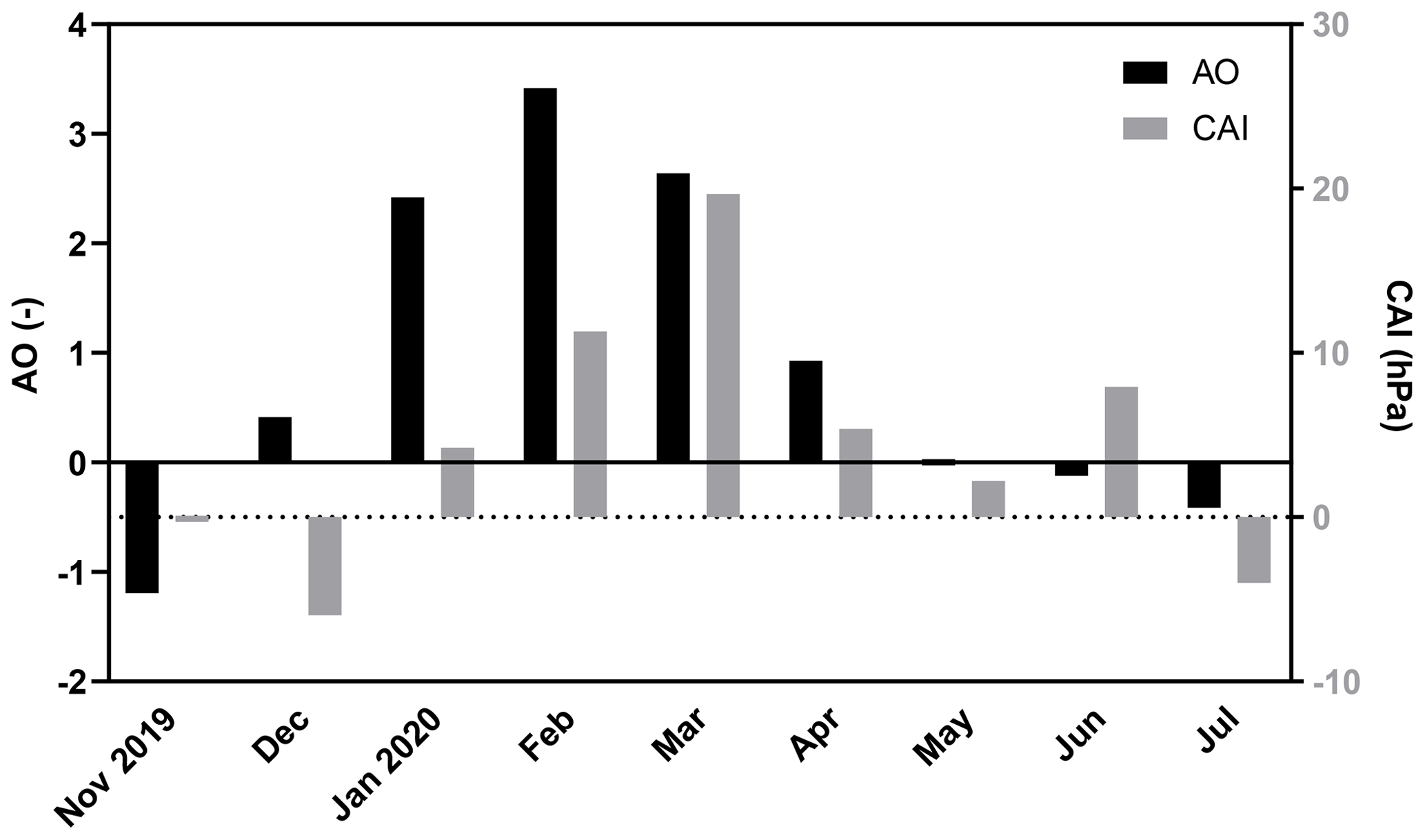
Figure A1Time series of the monthly AO index (black bar) and CAI (gray bar) from November 2019 to July 2020.
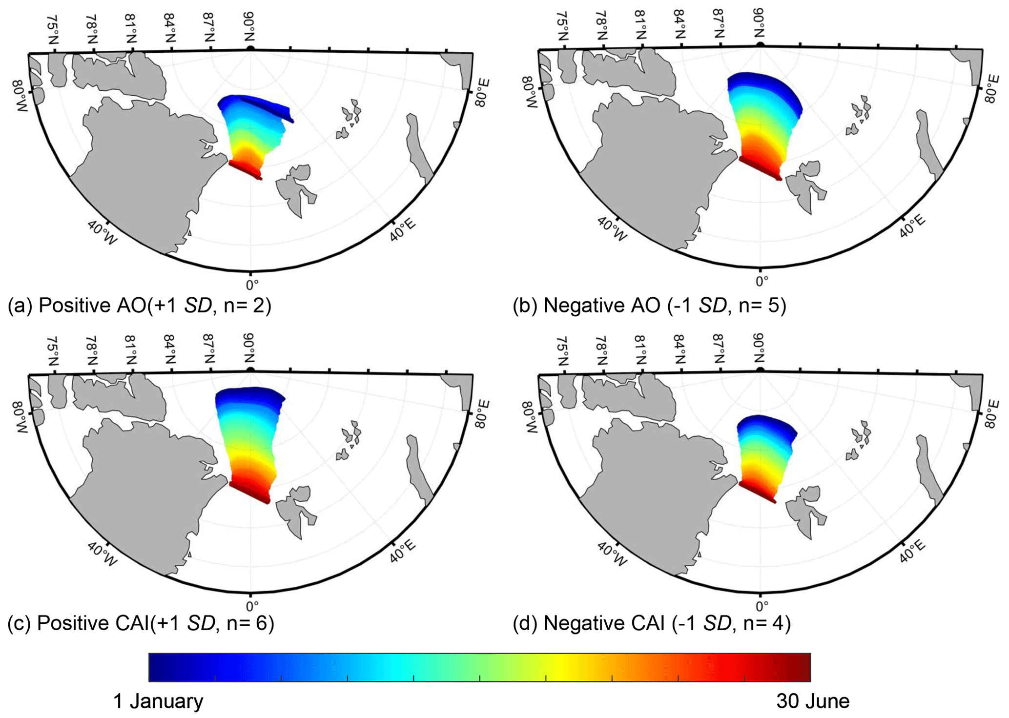
Figure A2Sea ice backward trajectories from the Fram Strait under the extremely positive and negative phases of the AO and CAI in 1988–2020. An extremely positive (negative) phase is defined as the value of the index higher (lower) than climatological values by 1 SD. Numbers represent the number of years with an extremely positive or negative phase of the atmospheric circulation indices. Color coding of the sea ice backward trajectories denotes the time from 1 January to 30 June.
Table A1Correlation coefficient (R) between monthly sea ice motion speed and wind speed in the Atlantic sector of the TPD for 1979–2020.
Note: significance levels are P<0.001 (bold), P<0.01 (italic), and P<0.05 (plain); n.s. denotes insignificant at the 0.05 level.
Table A2Consistency of reconstructed sea ice backward trajectories with buoy trajectories.
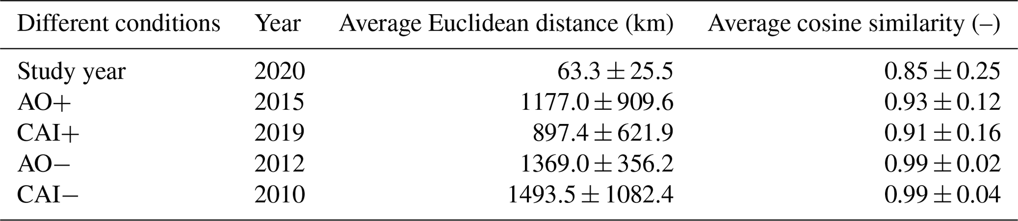
Table A3Synchronous correlation coefficient (R) between monthly sea ice area (SIA) and sea surface temperature (SST) in April, May, or June for 1982–2020.
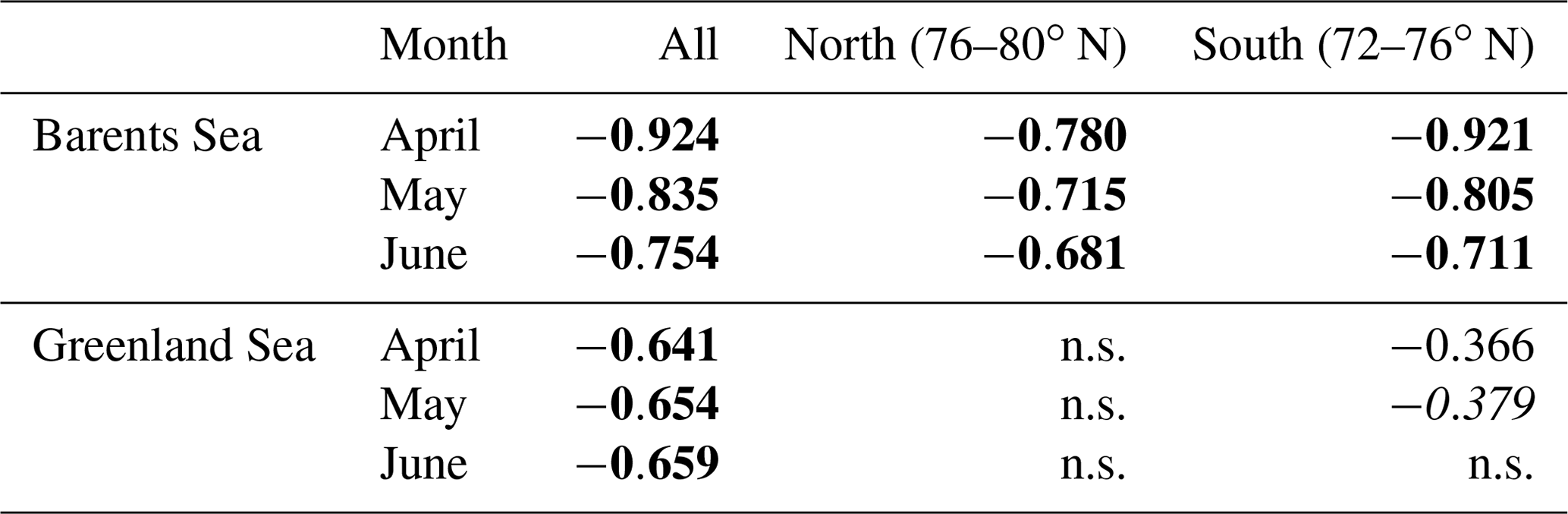
Note: significance levels are P<0.001 (bold), P<0.01 (italic), and P<0.05 (plain); n.s. denotes insignificant at the 0.05 level.
Table A4Lagging correlation coefficient (R) between monthly sea ice area (SIA) in April and sea surface temperature (SST) in May, June, or July for 1982–2020.
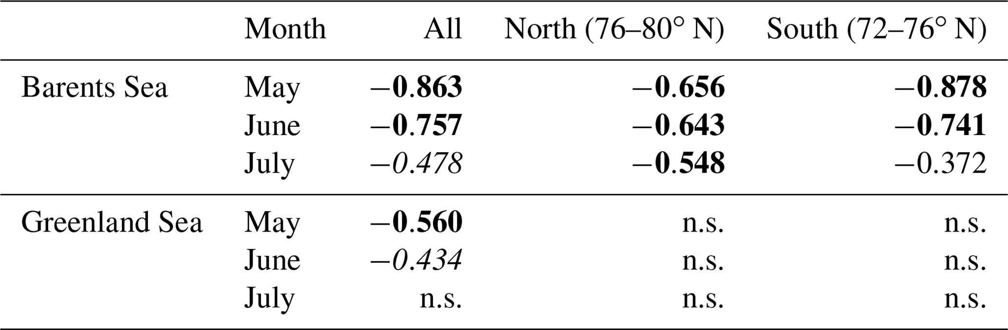
Note: significance levels are P<0.001 (bold), P<0.01 (italic), and P<0.05 (plain); n.s. denotes insignificant at the 0.05 level.
Table A5Correlation coefficient (R) between the latitude or longitude of endpoint of the sea ice backward trajectory from the Fram Strait and atmospheric circulation indices in 1988–2020.
Note: significance levels are P<0.001 (bold), P<0.01 (italic), and P<0.05 (plain); n.s. denotes insignificant at the 0.05 level.
Sea ice motion data from the NSIDC are available at https://doi.org/10.5067/INAWUWO7QH7B (Tschudi et al., 2019). NSIDC sea ice concentration data are obtained from https://doi.org/10.7265/efmz-2t65 (Meier et al., 2021). The MOSAiC buoy data are available at https://data.meereisportal.de/data/buoys/ (Grosfeld et al., 2023). The IABP buoy data were downloaded from https://iabp.apl.uw.edu/Data_Products/BUOY_DATA/ (Department of Fisheries and Oceans, Canada, 2021). Sea ice thickness was downloaded from merged CryoSat-2 and SMOS (https://data.seaiceportal.de/data/cs2smos_awi/v204/, Ricker et al., 2017) and PIOMAS (https://pscfiles.apl.uw.edu/zhang/PIOMAS/, Zhang and Rothrock, 2003). Sea surface temperature data are available at https://climatedataguide.ucar.edu/climate-data/sst-data-noaa-high-resolution-025x025-blended-analysis-daily-sst-and-ice-oisstv2 (Banzon et al., 2023). The ERA5 atmospheric reanalysis data were downloaded from https://doi.org/10.24381/cds.adbb2d47 (Hersbach et al., 2023). The AO index is available at https://www.cpc.ncep.noaa.gov/products/precip/CWlink/daily_ao_index/ao.shtml (National Weather Service Climate Prediction Center, 2023a). The NAO index was downloaded from https://www.cpc.ncep.noaa.gov/products/precip/CWlink/pna/nao.shtml (National Weather Service Climate Prediction Center, 2023b).
FZ carried out the analysis, processed the data, and prepared the manuscript. RL provided the concept, discussed the results, and revised the manuscript during the writing process. All authors commented on the manuscript and finalized this paper.
The contact author has declared that none of the authors has any competing interests.
Publisher's note: Copernicus Publications remains neutral with regard to jurisdictional claims made in the text, published maps, institutional affiliations, or any other geographical representation in this paper. While Copernicus Publications makes every effort to include appropriate place names, the final responsibility lies with the authors.
This research has been supported by the National Natural Science Foundation of China (grant nos. 41976219 and 42106231), the National Key Research and Development Program (grant nos. 2021YFC2803304 and 2018YFA0605903), and the Program of Shanghai Academic/Technology Research Leader (22XD1403600).
This paper was edited by Homa Kheyrollah Pour and reviewed by four anonymous referees.
Banzon, V., Smith., T. M., Steele, M., Huang, B., and Zhang, H.-M.: Improved estimation of proxy sea surface temperature in the Arctic, J. Atmos. Ocean. Technol., 37, 341–349, https://doi.org/10.1175/JTECH-D-19-0177.1, 2020.
Banzon, V., Reynolds, R., and National Center for Atmospheric Research Staff (Eds.): Last modified 2022-09-09, The Climate Data Guide: SST data: NOAA High-resolution (0.25x0.25) Blended Analysis of Daily SST and Ice, OISSTv2, https://climatedataguide.ucar.edu/climate-data/sst-data-noaa-high-resolution-025x025-blended-analysis-daily-sst-and-ice-oisstv2, last access: 29 October 2023.
Bi, H., Sun, K., Zhou, X., Huang, H., and Xu, X.: Arctic Sea ice area export through the Fram Strait estimated from satellite-based data: 1988–2012, IEEE J. Stars, 9, 3144–3157, https://doi.org/10.1109/jstars.2016.2584539, 2016.
Cai, L., Alexeev, V.A., and Walsh, J.E.: Arctic sea ice growth in response to synoptic- and large-scale atmospheric forcing from CMIP5 models, J. Climate, 33, 6083–6099, https://doi.org/10.1175/jcli-d-19-0326.1, 2020.
Cavalieri, D.J., Gloersen, P., and Campbell, W.J.: Determination of sea ice parameters with the Nimbus 7 SMMR, J. Geophys. Res.-Atmos., 89, 5355–5369, https://doi.org/10.1016/0198-0254(84)93205-9, 1984.
Comiso, J.C.: Characteristics of Arctic winter sea ice from satellite multispectral microwave observations, J. Geophys. Res.-Oceans, 91, 975–994, https://doi.org/10.1029/jc091ic01p00975, 1986.
Department of Fisheries and Oceans, Canada: https://iabp.apl.uw.edu/Data_Products/BUOY_DATA/, last access: 15 June 2021.
de Steur, L., Hansen, E., Mauritzen, C., Beszczynska-Moeller, A., and Fahrbach, E.: Impact of recirculation on the East Greenland Current in Fram Strait: Results from moored current meter measurements between 1997 and 2009, Deep-Sea Res. Pt. I, 92, 26–40, https://doi.org/10.1016/j.dsr.2014.05.018, 2014.
Dethloff, K., Maslowski, W., Hendricks, S., Lee, Y. J., Goessling, H. F., Krumpen, T., Haas, C., Handorf, D., Ricker, R., Bessonov, V., Cassano, J. J., Kinney, J. C., Osinski, R., Rex, M., Rinke, A., Sokolova, J., and Sommerfeld, A.: Arctic sea ice anomalies during the MOSAiC winter 2019/20, The Cryosphere, 16, 981–1005, https://doi.org/10.5194/tc-16-981-2022, 2022.
Dickson, R. R., Meincke, J., Malmberg, S. A., and Lee, A. J.: The “Great Salinity Anomaly” in the Northern North-Atlantic 1968–1982, Prog. Oceanogr., 20, 103–151, https://doi.org/10.1016/0079-6611(88)90049-3, 1988.
Dorr, J., Arthun, M., Eldevik, T., and Madonna, E.: Mechanisms of regional winter sea-ice variability in a warming Arctic, J. Climate, 34, 8635–8653, https://doi.org/10.1175/jcli-d-21-0149.1, 2021.
Grosfeld, K., Treffeisen, R., Asseng, J., Bartsch, A., Bräuer, B., Fritzsch, B., Gerdes, R., Hendricks, S., Hiller, W., Heygster, G., Krumpen, T., Lemke, P., Melsheimer, C., Nicolaus, M., Ricker, R., and Weigelt, M.: Online sea-ice knowledge and data platform <https://www.meereisportal.de>, Polarforschung, Bremerhaven, Alfred Wegener Institute for Polar and Marine Research & German Society of Polar Research, 85, 143–155, https://doi.org/10.2312/polfor.2016.011 (data available at: https://data.meereisportal.de/data/buoys/, last access: 30 October 2023), 2016.
Frey, K. E., Moore, G. W. K., Cooper, L. W., and Grebmeier, J. M.: Divergent patterns of recent sea ice cover across the Bering, Chukchi, and Beaufort seas of the Pacific Arctic Region, Prog. Oceanogr., 136, 32–49, https://doi.org/10.1016/j.pocean.2015.05.009, 2015.
Graham, R. M., Hudson, S. R., and Maturilli, M.: Improved performance of ERA5 in Arctic gateway relative to four global atmospheric reanalyses, Geophys. Res. Lett., 46, 6138–6147, https://doi.org/10.1029/2019gl082781, 2019.
Hastenrath, S. and Greischar, L.: The North Atlantic oscillation in the NCEP-NCAR reanalysis, J. Climate, 14, 2404–2413, https://doi.org/10.1175/1520-0442(2001)014<2404:TNAOIT>2.0.CO;2, 2001.
Hersbach, H., Bell, B., Berrisford, P., Hirahara, S., Horanyi, A., Munoz-Sabater, J., Nicolas, J., Peubey, C., Radu, R., Schepers, D., Simmons, A., Soci, C., Abdalla, S., Abellan, X., Balsamo, G., Bechtold, P., Biavati, G., Bidlot, J., Bonavita, M., De Chiara, G., Dahlgren, P., Dee, D., Diamantakis, M., Dragani, R., Flemming, J., Forbes, R., Fuentes, M., Geer, A., Haimberger, L., Healy, S., Hogan, R.J., Holm, E., Janiskova, M., Keeley, S., Laloyaux, P., Lopez, P., Lupu, C., Radnoti, G., de Rosnay, P., Rozum, I., Vamborg, F., Villaume, S., and Thepaut, J.-N.: The ERA5 global reanalysis, Q. J. Roy. Meteor. Soc., 146, 1999–2049, https://doi.org/10.1002/qj.3803, 2020.
Hersbach, H., Bell, B., Berrisford, P., Biavati, G., Horányi, A., Muñoz Sabater, J., Nicolas, J., Peubey, C., Radu, R., Rozum, I., Schepers, D., Simmons, A., Soci, C., Dee, D., Thépaut, J.-N.: ERA5 hourly data on single levels from 1940 to present, Copernicus Climate Change Service (C3S) Climate Data Store (CDS) [data set], https://doi.org/10.24381/cds.adbb2d47, 2023.
Huang, B., Liu, C., Banzon, V., Freeman, E., Graham, G., Hankins, B., Smith, T., and Zhang, H.M.: Improvements of the Daily Optimum Interpolation Sea Surface Temperature (DOISST) Version 2.1, J. Climate, 34, 2923–2939, https://doi.org/10.1175/JCLI-D-20-0166.1, 2021.
Hurrell, J. W.: Climate and climate change | Climate variability: North Atlantic and Arctic oscillation, in: Encyclopedia of Atmospheric Sciences, 2nd edn., edited by: North, G.R., Pyle, J., and Zhang, F., Academic Press, Oxford, 47–60, https://doi.org/10.1016/B978-0-12-382225-3.00109-2, 2015.
Krumpen, T., Birrien, F., Kauker, F., Rackow, T., von Albedyll, L., Angelopoulos, M., Belter, H. J., Bessonov, V., Damm, E., Dethloff, K., Haapala, J., Haas, C., Harris, C., Hendricks, S., Hoelemann, J., Hoppmann, M., Kaleschke, L., Karcher, M., Kolabutin, N., Lei, R., Lenz, J., Morgenstern, A., Nicolaus, M., Nixdorf, U., Petrovsky, T., Rabe, B., Rabenstein, L., Rex, M., Ricker, R., Rohde, J., Shimanchuk, E., Singha, S., Smolyanitsky, V., Sokolov, V., Stanton, T., Timofeeva, A., Tsamados, M., and Watkins, D.: The MOSAiC ice floe: sediment-laden survivor from the Siberian shelf, The Cryosphere, 14, 2173–2187, https://doi.org/10.5194/tc-14-2173-2020, 2020.
Krumpen, T., von Albedyll, L., Goessling, H. F., Hendricks, S., Juhls, B., Spreen, G., Willmes, S., Belter, H. J., Dethloff, K., Haas, C., Kaleschke, L., Katlein, C., Tian-Kunze, X., Ricker, R., Rostosky, P., Rückert, J., Singha, S., and Sokolova, J.: MOSAiC drift expedition from October 2019 to July 2020: sea ice conditions from space and comparison with previous years, The Cryosphere, 15, 3897–3920, https://doi.org/10.5194/tc-15-3897-2021, 2021.
Kwok, R.: Outflow of Arctic ocean sea ice into the Greenland and Barents Seas: 1979–2007, J. Climate, 22, 2438–2457, https://doi.org/10.1175/2008jcli2819.1, 2009.
Kwok, R., Cunningham, G., Wensnahan, M., Rigor, I., Zwally, H., and Yi, D.: Thinning and volume loss of the Arctic Ocean sea ice cover: 2003–2008, J. Geophys. Res.-Oceans, 114, https://doi.org/10.1029/2009jc005312, 2009.
Kwok, R., Spreen, G., and Pang, S.: Arctic sea ice circulation and drift speed: decadal trends and ocean currents, J. Geophys. Res.-Oceans, 118, 2408–2425, https://doi.org/10.1002/jgrc.20191, 2013.
Lei, R., Heil, P., Wang, J., Zhang, Z., Li, Q., and Li, N.: Characterization of sea-ice kinematic in the Arctic outflow region using buoy data, Polar. Res., 35, 22658, https://doi.org/10.3402/polar.v35.22658, 2016.
Lei, R., Gui, D., Hutchings, J.K., Wang, J., and Pang, X.: Backward and forward drift trajectories of sea ice in the northwestern Arctic Ocean in response to changing atmospheric circulation, Int. J. Climatol., 39, 4372–4391, https://doi.org/10.1002/joc.6080, 2019.
Lind, S., Ingvaldsen, R. B., and Furevik, T.: Arctic warming hotspot in the northern Barents Sea linked to declining sea-ice import, Nat. Clim. Change, 8, 634–639, https://doi.org/10.1038/s41558-018-0205-y, 2018.
Mayot, N., Matrai, P. A., Arjona, A., Belanger, S., Marchese, C., Jaegler, T., Ardyna, M., and Steele, M.: Springtime export of Arctic sea ice influences phytoplankton production in the Greenland Sea, J. Geophys. Res.-Oceans, 125, https://doi.org/10.1029/2019jc015799, 2020.
Meier, W. N., Fetterer, F., Windnagel, A. K., and Stewart, J. S.: NOAA/NSIDC Climate Data Record of Passive Microwave Sea Ice Concentration, Version 4, Boulder, NSIDC: National Snow and Ice Data Center, Colorado USA [data set], https://doi.org/10.7265/efmz-2t65, 2021.
Minnett, P. J. and Key, E. L.: Meteorology and atmosphere–surface coupling in and around polynyas, Elsev. Oceanogr. Serie., 74, 127–161, https://doi.org/10.1016/S0422-9894(06)74004-1, 2007.
Mori, M., Watanabe, M., Shiogama, H., Inoue, J., and Kimoto, M.: Robust Arctic sea-ice influence on the frequent Eurasian cold winters in past decades, Nat. Geosci., 7, 869–873, https://doi.org/10.1038/ngeo2277, 2014.
Mørk, T., Bohlin, J., Fuglei, E., Asbakk, K., and Tryland, M.: Rabies in the arctic fox population, Svalbard, Norway, J. Wildlife. Dis., 47, 945–957, https://doi.org/10.7589/0090-3558-47.4.945, 2011.
National Weather Service Climate Prediction Center of the National Oceanic and Atmospheric Administration: https://www.cpc.ncep.noaa.gov/products/precip/CWlink/daily_ao_index/ao.shtml, last access: September 2023a.
National Weather Service Climate Prediction Center of the National Oceanic and Atmospheric Administration: https://www.cpc.ncep.noaa.gov/products/precip/CWlink/pna/nao.shtml, last access: September 2023b.
Nicolaus, M., Riemann-Campe, K., Bliss, A., Hutchings, J. K., Granskog, M. A., Haas, C., Hoppmann, M., Kanzow, T., Krishfield, R. A., Lei, R., Rex, M., Li, T., and Rabe, B.: Drift trajectories of the main sites of the Distributed Network of MOSAiC 2019/2020, Alfred Wegener Institute, Helmholtz Centre for Polar and Marine Research, Bremerhaven, PANGAEA, https://doi.org/10.1594/PANGAEA.937204, 2021.
Onarheim, I. H., Eldevik, T., Smedsrud, L. H., and Stroeve, J. C.: Seasonal and regional manifestation of Arctic sea ice loss, J. Climate, 31, 4917–4932, https://doi.org/10.1175/jcli-d-17-0427.1, 2018.
Pabi, S., van Dijken, G. L., and Arrigo, K. R.: Primary production in the Arctic Ocean, 1998–2006, J. Geophys. Res.-Oceans, 113, C08005, https://doi.org/10.1029/2007JC004578, 2008.
Parkinson, C. L. and DiGirolamo, N. E.: Sea ice extents continue to set new records: Arctic, Antarctic, and global results, Remote Sens. Environ., 267, 112753, https://doi.org/10.1016/j.rse.2021.112753, 2021.
Parkinson, C. L. and Washington, W. M.: A large-scale numerical model of sea ice, J. Geophys. Res.-Oceans, 84, 311–337, https://doi.org/10.1029/JC084iC01p00311, 1979.
Peeken, I., Primpke, S., Beyer, B., Gutermann, J., Katlein, C., Krumpen, T., Bergmann, M., Hehemann, L., and Gerdts, G.: Arctic sea ice is an important temporal sink and means of transport for microplastic, Nat. Commun., 9, 1505, https://doi.org/10.1038/s41467-018-03825-5, 2018.
Peng, G., Meier, W. N., Scott, D. J., and Savoie, M. H.: A long-term and reproducible passive microwave sea ice concentration data record for climate studies and monitoring, Earth Syst. Sci. Data, 5, 311–318, https://doi.org/10.5194/essd-5-311-2013, 2013.
Polyakov, I. V., Ingvaldsen, R. B., Pnyushkov, A. V., Bhatt, U. S., Francis, J. A., Janout, M., Kwok, R., and Skagseth, Ø.: Fluctuating Atlantic inflows modulate Arctic atlantification, Science, 381, 972–979, https://doi.org/10.1126/science.adh5158, 2023.
Rahmstorf, S., Box, J. E., Feulner, G., Mann, M. E., Robinson, A., Rutherford, S., and Schaffernicht, E. J.: Exceptional twentieth-century slowdown in Atlantic Ocean overturning circulation, Nat. Clim. Change, 5, 475–480, https://doi.org/10.1038/NCLIMATE2554, 2015.
Reynolds, R. W., Smith, T. M., Liu, C., Chelton, D. B., Casey, K. S., and Schlax, M. G.: Daily high-resolution-blended analyses for sea surface temperature, J. Climate, 20, 5473–5496, https://doi.org/10.1175/2007jcli1824.1, 2007.
Ricker, R., Hendricks, S., Kaleschke, L., Tian-Kunze, X., King, J., and Haas, C.: A weekly Arctic sea-ice thickness data record from merged CryoSat-2 and SMOS satellite data, The Cryosphere, 11, 1607–1623, https://doi.org/10.5194/tc-11-1607-2017, 2017 (data available at: https://data.seaiceportal.de/data/cs2smos_awi/v204/, last access: 10 April 2022).
Rigor, I. G., Wallace, J. M., and Colony, R. L.: Response of sea ice to the Arctic Oscillation, J. Climate, 15, 2648–2663, https://doi.org/10.1029/1999gl002389, 2002.
Schlichtholz, P.: Subsurface ocean flywheel of coupled climate variability in the Barents Sea hotspot of global warming, Sci. Rep., 9, 1–16, https://doi.org/10.1038/s41598-019-49965-6, 2019.
Schweiger, A., Lindsay, R., Zhang, J. L., Steele, M., Stern, H., and Kwok, R.: Uncertainty in modeled Arctic sea ice volume, J. Geophys. Res.-Oceans, 116, C00D06, https://doi.org/10.1029/2011jc007084, 2011.
Shu, Q., Wang, Q., Song, Z., and Qiao, F.: The poleward enhanced Arctic Ocean cooling machine in a warming climate, Nat. Commun., 12, 2966, https://doi.org/10.1038/s41467-021-23321-7, 2021.
Siswanto, E.: Temporal variability of satellite-retrieved chlorophyll-a data in Arctic and subarctic ocean regions within the past two decades, Int. J. Remote. Sens., 41, 7427–7445, https://doi.org/10.1080/01431161.2020.1759842, 2020.
Smedsrud, L. H., Esau, I., Ingvaldsen, R. B., Eldevik, T., Haugan, P. M., Li, C., Lien, V. S., Olsen, A., Omar, A. M., and Otterå, O. H.: The role of the Barents Sea in the Arctic climate system, Rev. Geophy., 51, 415–449, https://doi.org/10.1017/cbo9780511535888.008, 2013.
Smedsrud, L. H., Halvorsen, M. H., Stroeve, J. C., Zhang, R., and Kloster, K.: Fram Strait sea ice export variability and September Arctic sea ice extent over the last 80 years, The Cryosphere, 11, 65–79, https://doi.org/10.5194/tc-11-65-2017, 2017.
Spreen, G., Kern, S., Stammer, D., and Hansen, E.: Fram Strait sea ice volume export estimated between 2003 and 2008 from satellite data, Geophys. Res. Lett., 36, L19502, https://doi.org/10.1029/2009GL039591, 2009.
Stroeve, J., Barrett, A., Serreze, M., and Schweiger, A.: Using records from submarine, aircraft and satellites to evaluate climate model simulations of Arctic sea ice thickness, The Cryosphere, 8, 1839–1854, https://doi.org/10.5194/tc-8-1839-2014, 2014.
Sumata, H., de Steur, L., Gerland, S., Divine, D. V., and Pavlova, O.: Unprecedented decline of Arctic sea ice outflow in 2018, Nat. Commun., 13, 1747, https://doi.org/10.1038/s41467-022-29470-7, 2022.
Thompson, D. W. J. and Wallace, J. M.: The Arctic Oscillation signature in the wintertime geopotential height and temperature fields, Geophys. Res. Lett., 25, 1297–1300, https://doi.org/10.1029/98gl00950, 1998.
Tschudi, M. A,, Meier, W. N., Stewart, J. S., Fowler, C., and Maslanik, J.: Polar Pathfinder Daily 25 km EASE-Grid Sea Ice Motion Vectors, Version 4, Boulder, NASA National Snow and Ice Data Center Distributed Active Archive Center, Colorado USA, [data set], https://doi.org/10.5067/INAWUWO7QH7B, 2019.
Tschudi, M. A., Meier, W. N., and Stewart, J. S.: An enhancement to sea ice motion and age products at the National Snow and Ice Data Center (NSIDC), The Cryosphere, 14, 1519–1536, https://doi.org/10.5194/tc-14-1519-2020, 2020.
Vihma, T., Tisler, P., and Uotila, P.: Atmospheric forcing on the drift of Arctic sea ice in 1989–2009, Geophys. Res. Lett., 39, L02501, https://doi.org/10.1029/2011gl050118, 2012.
Wang, X., Key, J., Kwok, R., and Zhang, J.: Comparison of Arctic sea ice thickness from satellites, aircraft, and PIOMAS data, Remote Sens., 8, 713, https://doi.org/10.3390/rs8090713, 2016.
Wang, Y., Bi, H., Huang, H., Liu, Y., Liu, Y., Liang, X., Fu, M., and Zhang, Z.: Satellite-observed trends in the Arctic sea ice concentration for the period 1979–2016, J. Oceanol. Limnol., 37, 18–37, https://doi.org/10.1007/s00343-019-7284-0, 2019.
Wassmann, P., Slagstad, D., and Ellingsen, I.: Primary production and climatic variability in the European sector of the Arctic Ocean prior to 2007: preliminary results, Polar. Biol., 33, 1641–1650, https://doi.org/10.1007/s00300-010-0839-3, 2010.
Zhang, F., Pang, X., Lei, R., Zhai, M., Zhao, X., and Cai, Q.: Arctic sea ice motion change and response to atmospheric forcing between 1979 and 2019, Int. J. Climatol., 42, 1854–1876, https://doi.org/10.1002/joc.7340, 2022.
Zhang, J. and Rothrock, D. A.: Modeling global sea ice with a thickness and enthalpy distribution model in generalized curvilinear coordinates, Mon. Weather. Rev., 131, 845–861, https://doi.org/10.1175/1520-0493(2003)131<0845:mgsiwa>2.0.co;2, 2003 (data available at: https://pscfiles.apl.uw.edu/zhang/PIOMAS/, last access: 31 December 2020).
Zhang, S., Gan, T., and Bush, A. B. G.: Variability of Arctic Sea Ice Based on Quantile Regression and the Teleconnection with Large-Scale Climate Patterns, J. Climate, 33, 4009–4025, https://doi.org/10.1175/JCLI-D-19-0375.1, 2020.