the Creative Commons Attribution 4.0 License.
the Creative Commons Attribution 4.0 License.
 | 20 Oct 2023
Monitoring glacier calving using underwater sound
Jarosław Tęgowski
Michał Ciepły
Małgorzata Błaszczyk
Jacek Jania
Mateusz Moskalik
Philippe Blondel
Grant B. Deane
Climate shifts are particularly conspicuous in glaciated areas. Satellite and terrestrial observations show significant increases in the melting and breakup of tidewater glaciers and their influence on sea level rise and ocean mixing. Increasing melt rates are creating an urgency to better understand the link between atmospheric and oceanic conditions and glacier frontal ablation through iceberg calving and melting. Elucidating this link requires a combination of short- and long-timescale measurements of terminus activity. Recent work has demonstrated the potential of using underwater sound to quantify the time and scale of calving events to yield integrated estimates of ice mass loss (Glowacki and Deane, 2020). Here, we present estimates of subaerial calving flux using underwater sound recorded at Hansbreen, Svalbard, in September 2013 combined with an algorithm for the automatic detection of calving events. The method is compared with ice calving volumes estimated from geodetic measurements of the movement of the glacier terminus and an analysis of satellite images. The total volume of above-water calving during the 26 d of acoustical observation is estimated to be m3, whereas the subaerial calving flux estimated by traditional methods is m3. The results suggest that passive cryoacoustics is a viable technique for long-term monitoring of mass loss from marine-terminating glaciers.
- Article
(7521 KB) - Full-text XML
- BibTeX
- EndNote


The loss in the mass of the Greenland ice sheet, which increased from 41±17 Gt yr−1 in 1990–2000 to 286±20 Gt yr−1 in 2010–2018 (Mouginot et al., 2019), is of great concern. Greenland's contribution to sea level rise by the end of the 21st century relative to 1995–2014 is estimated to be 0.06 (0.01 to 0.10) m and 0.08 (0.04 to 0.13) m under SSP1–2.6 and SSP2–4.5 shared socioeconomic pathways, respectively (IPCC, 2023); these estimates exclude peripheral glaciers and ice caps. Moreover, recent studies have shown that the accelerated break-up and melting of Antarctica – the largest reservoir of fresh water on Earth – will be responsible for a sea level rise of at least 0.5 cm yr−1 by 2100 (Paolo et al., 2015; DeConto et al., 2021). Despite these concerning numbers, the loss of land-based ice in the coming decades could be under-predicted. For example, Greenland and Antarctic ice sheets likely have tipping points at around 1.5–2.0 ∘C of a mean global temperature increase compared to the pre-industrial era (Pattyn et al., 2018; Pattyn and Morlighem, 2020; Noël et al., 2021). Glaciers and ice caps in Patagonia, Svalbard, Antarctic Peninsula, and other glaciated regions are also losing mass at an accelerated pace (IPCC, 2023). The severe consequences of sea level rise and regional freshening of the ocean combined with current uncertainties in models of glacial retreat suggest that long-term monitoring of glacial stability is both important and urgent (Straneo et al., 2019).
There are many challenges to the long-term monitoring of glaciers and ice shelves. Polar regions are remote and subject to darkness for up to 6 months a year. Moreover, capturing the episodic character of ice breakup usually requires sub-second temporal resolution over year-long timescales. Despite a suite of current techniques, including satellite technology (Smith et al., 2020; Podgórski and Pętlicki, 2020), camera observations (Medrzycka et al., 2016; How et al., 2019), terrestrial laser scanning (Pętlicki and Kinnard, 2016; Podgórski et al., 2018), ground-based radar imaging (Xie et al., 2018; Walter et al., 2020), sonar scans (Sugiyama et al., 2019; Sutherland et al., 2019), and seismic records (Köhler et al., 2016; Podolskiy and Walter, 2016), continuous and long-term observations of the scale and rapidity of ice loss in logistically challenging polar regions are still urgently required (Straneo et al., 2013).
There are three major processes driving mass loss from marine-terminating glaciers: surface melting, submarine melting, and calving, which is the mechanical loss of ice from the edges of glaciers or ice shelves (Benn et al., 2007b). Calving and submarine melting – the two mechanisms of frontal ablation – are very difficult to quantify separately (Truffer and Motyka, 2016). Calving is responsible not only for ice loss itself but also for profound changes in ocean mixing, which affect sea ice formation and marine productivity. Meredith et al. (2022) have recently demonstrated that internal tsunamis triggered by calving events are important drivers of regional shelf mixing. Calving is a complex process that depends on a broad range of factors, including but not limited to (i) changes in glacier surface velocity along the flow line (longitudinal stretching), (ii) submarine melting of the terminus (undercutting), and (iii) geometry of the glacier–bay system (van der Veen, 2002; Benn et al., 2007b). This complexity makes the formulation of a general model of how calving changes in response to warming conditions a challenging task that requires long-term, temporally resolved datasets (e.g., van der Veen, 2002; Benn et al., 2007a).
Passive cryoacoustics, the use of ambient sounds to study ice–ocean interactions in polar regions, has the potential to provide the long-term, temporally resolved time series required for calving model development and monitoring the long-term stability of glaciers and ice sheets (see discussion in Glowacki and Deane, 2020), provided that the geophysical signals of relevance can be recovered from the properties of the sound. The field of ambient noise oceanography is well-established and has been used to recover signals such as wind speed and precipitation, for example (e.g., Nystuen, 1986; Vagle et al., 1990). The use of passive acoustics in polar regions is a relatively new field, still under development (Glowacki et al., 2015; Pettit et al., 2015; Deane et al., 2019; Yun et al., 2021; Podolskiy et al., 2022).
A recent milestone has been the demonstration that the mass of a calving iceberg can be estimated from its underwater impact noise with the sea surface (Glowacki and Deane, 2020). The method exploits the observed power-law relationship between the kinetic energy of a falling ice block immediately prior to impact and the resulting sound energy produced. The kinetic energy of an impacting block can be estimated from the sound energy radiated provided that propagation losses between the block and the recording location can be estimated. Because the drop height of icebergs is limited by the vertical extent of the terminus, the estimate of impact energy can then be converted into a block mass using what Glowacki and Deane (2020) call a “mass-weighted average drop height”, .
Here we demonstrate the use of passive cryoacoustics to monitor the subaerial calving flux from a tidewater glacier in southwestern Spitsbergen over 26 d of continuous measurements using algorithms for the automatic detection of calving events and the removal of contaminating signals, such as iceberg disintegration. Acoustic estimates of the ice volume loss are compared with concurrent camera and satellite observations.
The site for this study is Hansbreen, a retreating, grounded, polythermal tidewater glacier terminating in Hornsund fjord, Svalbard. Its calving mode, believed to be driven by melt undercutting and many relatively small calving events from above the water surface (Pętlicki et al., 2015), provides a challenging test case for camera and satellite estimates of mass flux.
A map of the study site and an example photograph of the terminus of Hansbreen are shown in Fig. 1. Hansbreen covers an area of around 54 km2, is more than 15 km long (Błaszczyk et al., 2013), and has a 1.5 km wide active calving front with an average height of around 40 m (Błaszczyk et al., 2009, 2021), which is approximately 30 %–40 % of the total ice thickness. The glacier surface flow is dominated by basal motion in the ablation area (Vieli et al., 2004), and the mean annual flow velocity near the terminus and its calving flux is estimated to be 177 m yr−1 and 35×106 m3 yr−1, respectively (Błaszczyk et al., 2019).
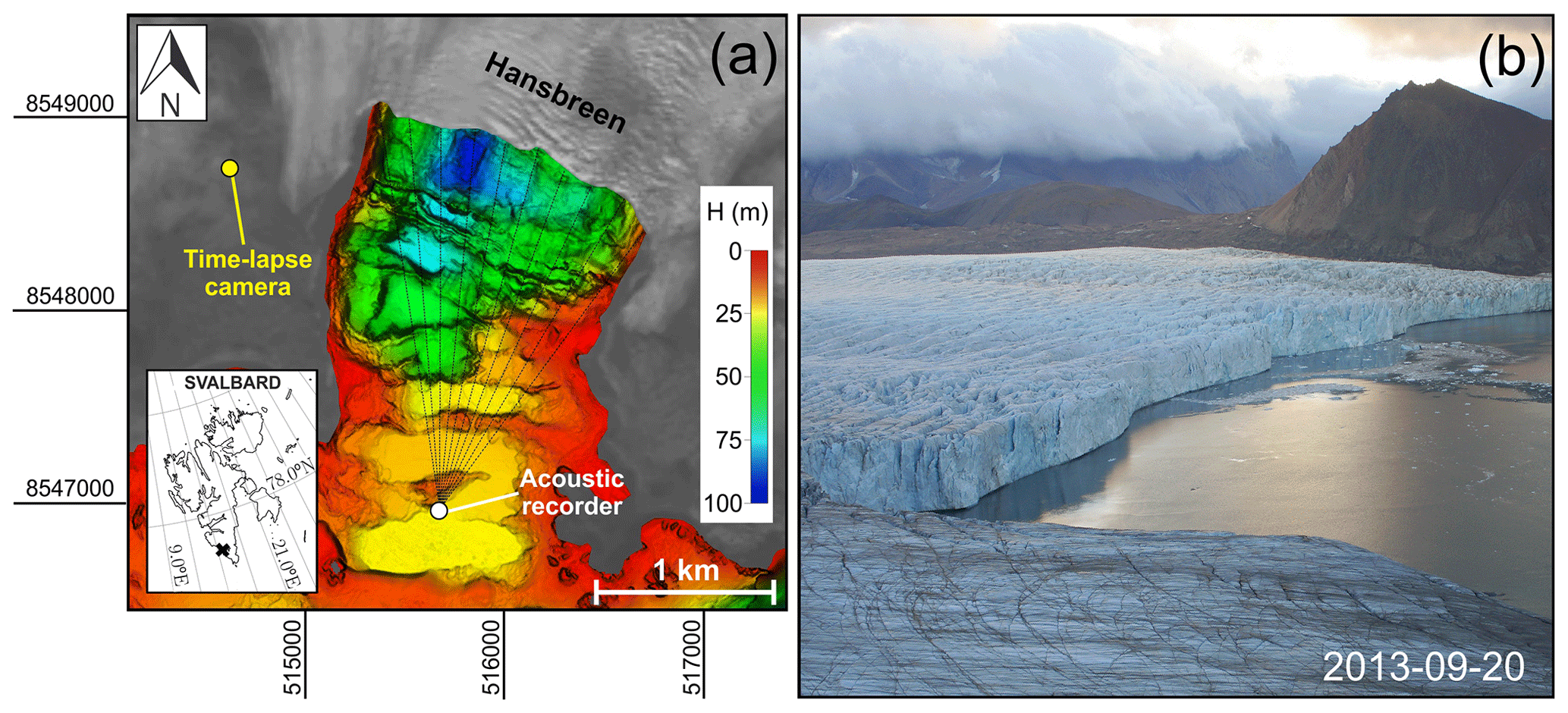
Figure 1(a) Map of the study site and (b) example image of the Hansbreen terminus. Locations of the time-lapse camera and the acoustic buoy are marked with yellow and white font, respectively. The map is in UTM projection system (zone 33N). The dashed black lines show different propagation transects that were used for estimating the noise transmission loss. Landsat 8 satellite data collected on 11 September 2013, courtesy of the US Geological Survey, Department of the Interior. Bathymetric data provided by (1) the Norwegian Hydrographic Service under the permit no. 13/G722, issued to the Institute of Geophysics Polish Academy of Sciences, and (2) the Faculty of Natural Sciences, Institute of Earth Sciences, University of Silesia in Katowice, Sosnowiec, Poland (Błaszczyk et al., 2021).
Both glacial behavior (Pętlicki et al., 2015; Błaszczyk et al., 2021) and the propagation of calving sounds (Glowacki et al., 2016) are sensitive to the space and time-varying thermohaline structure of water masses in the bay, which were characterized with CTD casts. The water temperature and salinity (practical salinity units) in the center of the bay ranged from −1.8 to more than 2.0 ∘C and from 30 to almost 35 during 2015 and 2016 (Moskalik et al., 2018). Sound propagation also depends on water depth, which drops to almost 100 m along a transect parallel to the glacier terminus (see Fig. 1a). The morphology of the bay varies greatly, with numerous moraines and flat areas created during the retreat of Hansbreen (Moskalik et al., 2018).
Glowacki and Deane (2020) have shown that the mass of individual icebergs can be estimated from the sound they produce when they impact the sea surface. In that study, 169 subaerial calving events from Hansbreen were manually identified in time-lapse photography and simultaneous recordings of the ambient sound, both made roughly 1 km from the glacier terminus. Despite significant variability in the total sound energy produced by an impact event for icebergs of comparable size, Monte Carlo simulations of ensemble time series show that accurate estimates of subaerial calving flux can be made if sufficient events are averaged (40 events for 20 % standard error for Hansbreen).
The manual identification of calving events using time-lapse photography and underwater sound is accurate but too labor intensive to be seriously considered for long-term datasets. This issue is addressed here by developing algorithms for the automatic detection of ice impact noise in the ambient sound recordings and rejection of interfering events, such as the disintegration of icebergs in the bay to obtain accurate estimates of ice loss from the terminus of Hansbreen due to calving.
The automatic detection of calving events is based on the observation that the ambient sound field in a glacial bay is composed of two distinct categories of sound sources: (1) sources that radiate noise with statistical properties that are stationary on the timescale of a calving event (such as melting glacier ice, for example) and (2) transient sources, like calving, superposed on this stationary background. During periods when noise in the bay is dominated by ice melting and calving, the signal during a 10 min data segment has the form of a wandering baseline punctuated at random intervals by hill-shaped increases as calving events occur. The level and noisiness of the baseline varies over time due to changes in the rate of ice melting on the glacier terminus, proximity to the hydrophone of icebergs drifting in the bay, and variable acoustic propagation through the bay. These varying conditions are unpredictable and require the selection of a baseline level and event detection threshold that is adaptable.
The signal processing scheme for event detection works as follows. A 10 min segment of ambient sound is transformed into a spectrogram. The sound power, Pb, between a lower and upper frequency band, f0=30 Hz to f1=100 Hz, is then computed using
where Pxx is the power spectral density estimate for the noise segment and the operators M(Θ) and B(Ω) are the filters described below. The selection of frequency limits is motivated by previous analyses of the calving noise presented in Glowacki and Deane (2020) and Glowacki (2020) (see Appendix A: Materials and methods for more details). The integral in Eq. (1) is calculated using the trapezoidal rule. The filter M(Θ) is a median filter of the order of Θ=7 and is useful for eliminating loud, impulsive noise sources that are too short to be calving noise. A boxcar filter B(Ω) of length Ω=32 points is applied to further reduce the effects of impulsive noise sources and random variations in noise power.
A baseline power for the noise in the absence of calving, Pbase, is taken to be the median of the probability density distribution of Pb. A threshold of detection, Pthres, is then selected to be 1.5 times the largest value of Pb with relative likelihood
where β=5. This constant plays a central role in detector performance and is referred to as the “detection factor”. It should be borne in mind, however, that different study sites and experiment geometries may require different constants and thresholds for effective calving detection (see Appendix A: Materials and methods).
Calving events are identified as continuous periods of time when Pb exceeds Pthres. The detection algorithm is based on the idea that calving events are relatively rare within 10 min intervals, and periods of time containing many successive events will drive the algorithm to select only the most energetic of them (see Appendix A: Materials and methods).
An example of the detector output is shown in Fig. 2. Figure 2a shows 1 min of ambient sound energy containing a calving event, presented in dB re 1 µPa2 Hz−1 as a function of frequency and time. Figure 2b shows the output from the band-pass and median filters, the baseline level, the threshold level, and detection of the calving event. The detector was run on the 26 d of recordings, resulting in the detection of 4258 events (see Appendix A: Materials and methods for a discussion of how sensitive the algorithm is to the choice of detection factor). The primary outputs of the event detector are the event start and end times, t0 and t1.
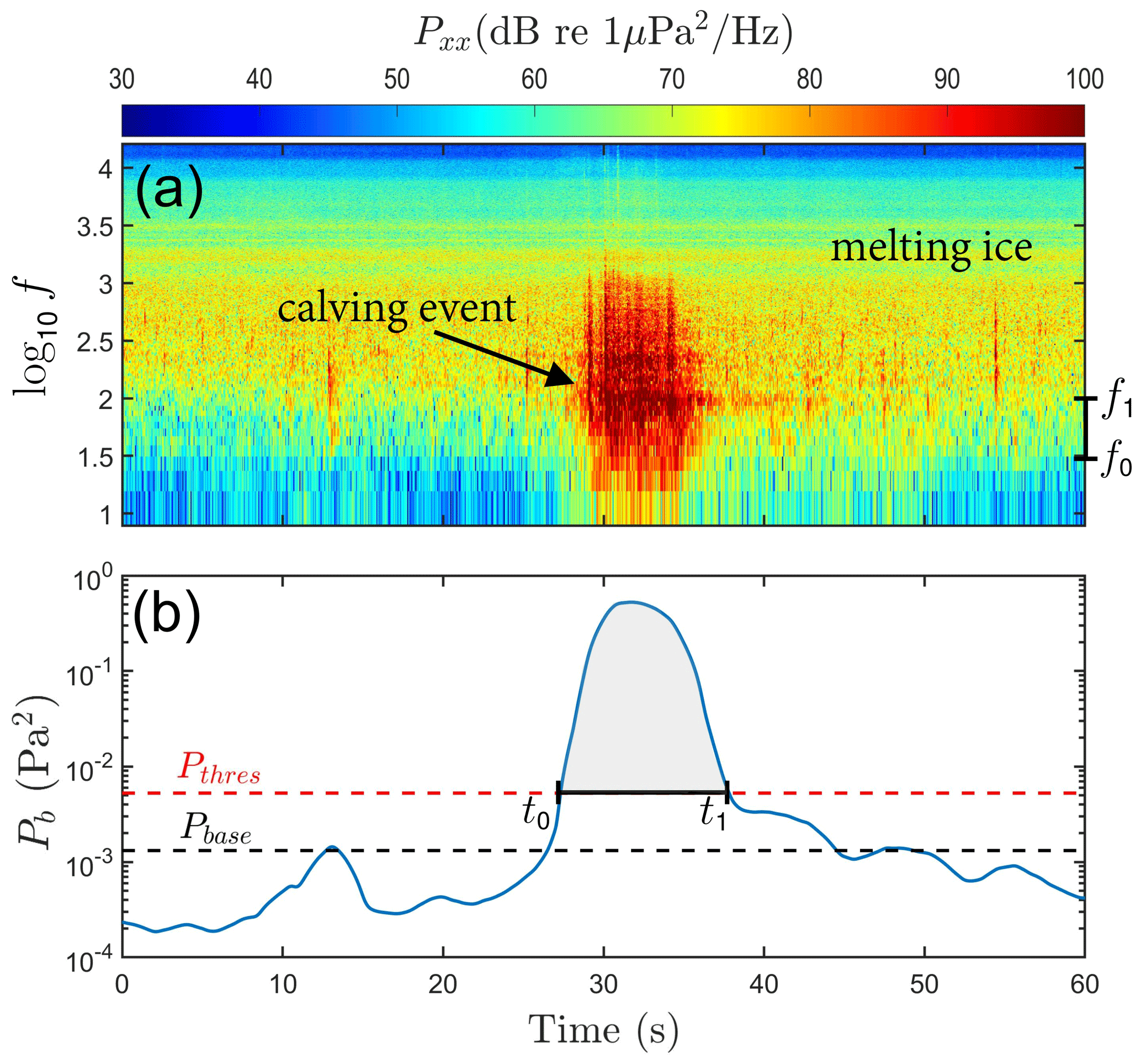
Figure 2Calving detector explained. (a) A spectrogram of the sound produced by a calving event within the background noise radiated by the melting terminus of Hansbreen. The frequencies f0 and f1 on the right-hand side of the plot denote the lower and upper limits of the detection frequencies (see text for details). (b) Noise power from the spectrogram above, integrated from f0 to f1 and filtered. The calving event is detected when the noise power exceeds the power threshold, Pthres, as annotated by t0 and t1. The threshold power is based on the baseline power, Pbase, which is determined from a statistical analysis of the sound (see text for details).
The problem remains of identifying events that were detected as calving but which are not. Visual inspection of noise spectrograms combined with listening to the corresponding sound recordings revealed two major sources of interfering sounds: (1) the disintegration of icebergs close to the acoustic buoy, which sounds like a calving event because the iceberg sheds blocks of ice into the water as it disintegrates, and (2) water movement around the hydrophone (flow noise). Other interfering events include calving from the terminus with highly energetic contacts between the falling iceberg and the terminus, icebergs colliding with other ice pieces that occupy the sea surface along the terminus, and calving events involving ice block rotation in the air, resulting in large contact area between the iceberg and sea surface leading to atypical sound production. Although all these events represent a challenge for the technique, the most concerning are the flow noise and disintegrating icebergs, which can be confused with very large calving events. The interfering events must be removed from the calving inventory before the ice mass loss is estimated. To deal with the misclassification problem, we take two steps.
First, we take advantage of the fact that submarine melting of glacier ice also generates underwater noise due to the impulsive release of pressurized air bubbles into the water (Urick, 1971; Deane et al., 2014; Pettit et al., 2015). Glowacki et al. (2018) have demonstrated that the melt noise has an α-stable distribution. This should not come as a surprise as stable distributions allow skewness and heavy tails (Nolan, 2021). Importantly, the characteristic exponent of the α-stable distribution – a parameter that determines the heaviness of the tails – indicates proximity to a melting source. When the melting iceberg is close to the receiver, the underwater noise at frequencies 1–10 kHz is more impulsive and the exponent α deviates from 2. Here, we assume the following: if α<1.95 for the noise segment immediately preceding the calving noise, there is a high likelihood that the corresponding event detected by the automated algorithm is in fact an iceberg disintegrating close to the hydrophone. Such events are discarded. In this case, 875 events were removed from the inventory. It should be borne in mind, however, that the disintegration of icebergs located at a similar distance from the hydrophone as the glacier terminus can still be confused with calving events. This issue cannot be addressed in the present study because of the limited view and low temporal resolution of the time-lapse camera and inability to estimate the noise directionality (single-channel recordings). In future studies, two or more hydrophones could be used to identify and discard noise signals not related to the calving activity.
Second, the noise segments are occasionally contaminated with flow noise, which originates from water turbulence advected past the hydrophone and is most pronounced at frequencies below ∼50 Hz. An overlap in frequency between the calving detector band (30–100 Hz) and the flow noise (2–50 Hz) can result in false classifications of the episodes of intense water flow around the hydrophone as calving events. To deal with this issue, we discard all events for which the ratio between the average power spectral density at 2–30 and 50–1000 Hz is higher than or equal to 1. This procedure is based on the observation that calving noise extends into the 50–1000 Hz band, whereas flow noise is most pronounced at frequencies below 30 Hz. Using these criteria, 328 misclassifications were identified and manually validated by listening to the selected noise segments and visual inspections of spectrograms. In total, 1128 events were discarded due to the fact that 75 events were identified as both flow noise and iceberg disintegration.
One issue remains, which is the fact that some fraction of the event signals found come from submarine calving events. Submarine calving events are a problem because the parameters in the power-law relationship between the energy of noise production and kinetic energy of block impact are for subaerial events and will not apply to submarine events (Glowacki and Deane, 2020). Thus any submarine events included in the calving inventory will not have their volume calculated correctly. Moreover, even if their volume were calculated correctly, they are not detected by the camera observations for this study. The analysis of calving flux from submarine events would first require new calibration data (see Sect. A4 in Appendix A for more details).
The total number of submarine calving events in the present inventory is not expected to be large. Reported statistics of submarine calving from other study sites show that such events are typically much less common than subaerial calving (Minowa et al., 2018; Köhler et al., 2019; How et al., 2019). Glowacki (2022) estimated that submarine calving events at Hansbreen are 8–10 times less frequent than subaerial events. It must be noted, however, that the low rate of occurrence of submarine calving is offset by the fact that submarine events often produce the biggest icebergs (Warren et al., 1995; Motyka, 1997; O'Neel et al., 2007; Glowacki, 2022). Consequently, attributing this component of the total calving flux to subaerial events may introduce an error disproportionately large relative to their number. In response to this problem, a new semi-automatic method for distinguishing submarine and subaerial calving events was recently proposed (Glowacki, 2022). However, there is no way at the present time to classify calving styles from sound recordings using fully automated methods. The time and frequency structure of the underwater noise from submarine and subaerial calving differs significantly (Glowacki, 2022); for example, the underwater noise from submarine calving typically has longer duration, with individual sound-source mechanisms separated by the quiescent periods. As a result, a universal calving detector should (i) take into account the differences in time and frequency structure of the calving noise and (ii) be validated with high-frequency time-lapse images synchronized with long-term acoustic recordings; this task is beyond the scope of the present study. Keeping this limitation in mind, the section that follows will explain how the subaerial calving flux can be estimated acoustically, with an assumption that all detected events are subaerial.
Following event detection, the next step is to compute the total noise energy radiated by the calving event at a standard reference distance of 1 m, Eac,imp. This step requires the calculation of the time- and frequency-integrated energy of the calving noise. The energy of the impact sound radiated by a falling ice block can be expressed in terms of the observed sound energy by accounting for propagation effects and the addition of background noise using the following:
where ρw is the water density, cw is the sound speed, f0=30 Hz and f1=100 Hz are lower and upper frequency limits, t0 is the start time of the calving event determined from the event detector, is the calving signal duration, where t1 is the end time of the calving signal, and TL is the frequency-dependent transmission loss between the hydrophone and the point of ice block impact (in dB). The acoustic signal is integrated over the surface area of a unit sphere (4π) to obtain total noise energy in joules. The two integrals over time, and , are the frequency spectral densities of the calving noise plus background noise and background noise alone, respectively. The transmission loss is calculated using the standard numerical code RAM (Collins, 1993) (see Appendix A: Materials and methods for further details).
In the next step, the kinetic energy of the falling block of ice, Eimp, is calculated from the total impact sound energy radiated into the bay, Eac,imp, using the power-law relationship:
where , κ=0.18 and are constants determined using the calibration dataset collected in 2016 (Glowacki and Deane, 2020; see Appendix A: Materials and methods for details). Finally, the iceberg volume is calculated as
where M is the iceberg mass, ρi=917 kg m−3 is assumed ice density, g=9.81 m s−2 is the acceleration due to gravity, and m is the mass-weighted average drop height estimated for the terminus of Hansbreen (Glowacki and Deane, 2020).
Figure 3 shows a comparison of two time series: (i) subaerial calving flux derived from iceberg impact noise and (ii) terminus area loss estimated from camera observations over the 26 d of analysis (see Appendix A: Materials and methods). The ice volume loss was calculated every 3 h, which is the sampling time of the camera system. Both data streams show variability between samples and between each other. This is to be expected; Glowacki and Deane (2020) demonstrated that the acoustic method is accurate if sufficient calving events are averaged but significant variability is observed in the signal between blocks of comparable volume. Moreover, camera observations are sensitive not only to weather conditions but also to the location of calving events due to the irregular shape of the terminus and oblique angle of view (see Fig. 1b). However, there is a clear relationship between the acoustic measurements of subaerial calving fluxes and the time-lapse observation of the terminus area loss, despite the limitations of both methods. The Pearson's correlation coefficient between the two data streams smoothed with a 1 d running average is 0.6. Comparing 2D terminus area loss from images with 3D ice volume loss from acoustic recordings may introduce some artifacts. Nevertheless, the purpose of our approach was to demonstrate the general strong correspondence of calving activity at Hansbreen determined from time-lapse images and underwater noise recordings and thus the overall complementary suitability of this methodology. Computing glacier volume loss due to calving from time-lapse images taken in the study period is problematic for two major reasons: highly oblique camera view and relatively long time intervals between consecutive images (3 h). The latter can easily lead to the classification of several low-magnitude calving events originating in the same sector of the calving front as a single big event. In such a case, the volume loss calculated from the area loss would be largely overestimated; therefore, to better represent the real calving activity, we have decided to stop the image analysis at the calculation of the terminus area loss.
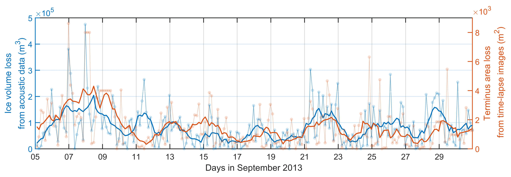
Figure 3A comparison of ice volume loss derived from iceberg impact noise and terminus area loss from camera observations. The ice volume loss was calculated every 3 h, which is the sampling time of the camera system. The thick lines show the two data streams smoothed with 1 d running average.
The question now is the following: how do the acoustic measurements of the total subaerial calving flux compare to results obtained with more traditional methods? The cumulative subaerial ice volume loss over the 26 d of observation is m3 from the acoustic measurements and m3 from satellite data combined with stake measurements of the glacier velocity. The discrepancy may be due to several reasons. First, any submarine calving events are treated as subaerial in the acoustic analysis. Consequently, the ice volume loss from acoustics is almost certainly overestimated. This issue has been addressed recently by Glowacki (2022) and can be incorporated into a long-term analysis once a method is developed for the automatic detection of submarine calving. Second, the power-law relationship in Eq. (4) is based on the calibration dataset that does not cover the full range of impact noise energies observed in 2013 data (see Fig. A2 and discussion in Appendix A: Materials and methods). Third, the location of the hydrophone – far from the terminus and in shallow water – was unfavorable because the propagation conditions of the calving noise are very different for different segments of the terminus (see the variable bathymetry along the dashed black lines in Fig. 1a), which has a large effect on the transmission losses of low-frequency sounds in a glacial bay (Glowacki and Deane, 2020). Finally, stake measurements of the ice velocity that were used to calculate subaerial calving flux from satellite images are from August 2013, which is a month before the acoustic data were collected. It is likely that Hansbreen accelerated in September due to heavy rainfall events; such “autumn acceleration” has been reported for other tidewater glaciers in Svalbard (e.g., Luckman et al., 2015; Schellenberger et al., 2015). Moreover, stake measurements do not capture ice velocity variations along the glacier terminus. The results of the experiment presented here are encouraging, given the limitations listed above and completely independent nature of the methods used to make the measurements.
The study of Glowacki and Deane (2020) demonstrated the potential for underwater ambient sound in glacial terminal bays to provide estimates of subaerial calving flux. Guided by this new opportunity, an impact-to-noise conversion model has been applied here to a roughly 1-month long continuous recording of ambient sound in the bay of Hansbreen in Svalbard to estimate subaerial calving flux. Good agreement is found between acoustic measurements of ice volume loss and the camera observations of the terminus area loss. The cumulative subaerial calving flux estimated using the acoustic approach is higher than the ice loss derived using a pair of satellite images combined with stake measurements of the glacier velocity. Clearly, the acoustic method requires further improvements, but the results are encouraging, especially as acoustic recorders are increasingly deployed in the Arctic for other studies, such as studies of biodiversity or human impacts like shipping, and they can be harnessed to also provide measurements of any neighboring glaciers. This study reinforces the idea that passive underwater acoustics offers a new and viable method for monitoring mass loss from marine-terminating glaciers and ice shelves.
The development of algorithms for the automated detection of calving events and the removal of interfering events, such as disintegrating icebergs and flow noise, creates the possibility of monitoring the stability of tidewater glacier termini and ice shelves over long timescales. We envision a scenario where a number of relatively inexpensive autonomous underwater recording systems are deployed over year-long intervals around the termini of selected glaciers on a recurrent schedule. There are many possible selection criteria, but we are interested in (i) glaciers that contribute the most to the sea level rise and stability of major ice sheets and (ii) glaciers that are scientifically important for other reasons (surging, collapsing rapidly, located close to major infrastructure, etc.). The analysis of the resulting signals would eventually allow glacial stability to be monitored over decadal and longer timescales. Concurrent measurements of relevant environmental drivers, such as water temperature, insolation, and precipitation for example, could provide important insights into the processes controlling terminus ablation. Moreover, long-term acoustic monitoring programs could also help to better understand the impact of calving events on ocean stratification, structure and functioning of marine ecosystems, and glacier dynamics itself.
Personal experience making long-term recordings in the Arctic has taught us that not all deployed recording systems are recovered. It is therefore essential to keep the unit cost of recording systems low to allow for as much redundancy as possible within a fixed budget. Power consumption and data storage are two important drivers of cost. Requirements for both of these factors can be reduced by recording ambient sound on a fixed schedule or recording whenever the sound level exceeds a preset threshold. These two possibilities will now be discussed.
Figure 4 shows the effect of recording coverage on the estimated total number of calving events (A) and cumulative ice volume loss (B) over the study period. A continuous acoustic record corresponds to Δ=0 %. Periods of active recording change from 1 h d−1 (≈4 %) to full coverage. Final estimates are derived proportionally; i.e., values obtained for 10 % and 20 % coverage are multiplied by 10 and 5, respectively. The specific hours of recordings during a day are selected repeatedly using all possible combinations, creating a distribution of outputs for the chosen value of coverage. The event count is much less sensitive to the recording schedule than the subaerial calving flux. Nevertheless, 1 standard deviation of the estimated ice volume loss at 30 % coverage is within 10 % of the reference value. This result demonstrates the possibility of significant reduction in recording time (by 70 %) with relatively low increase in the resulting error.
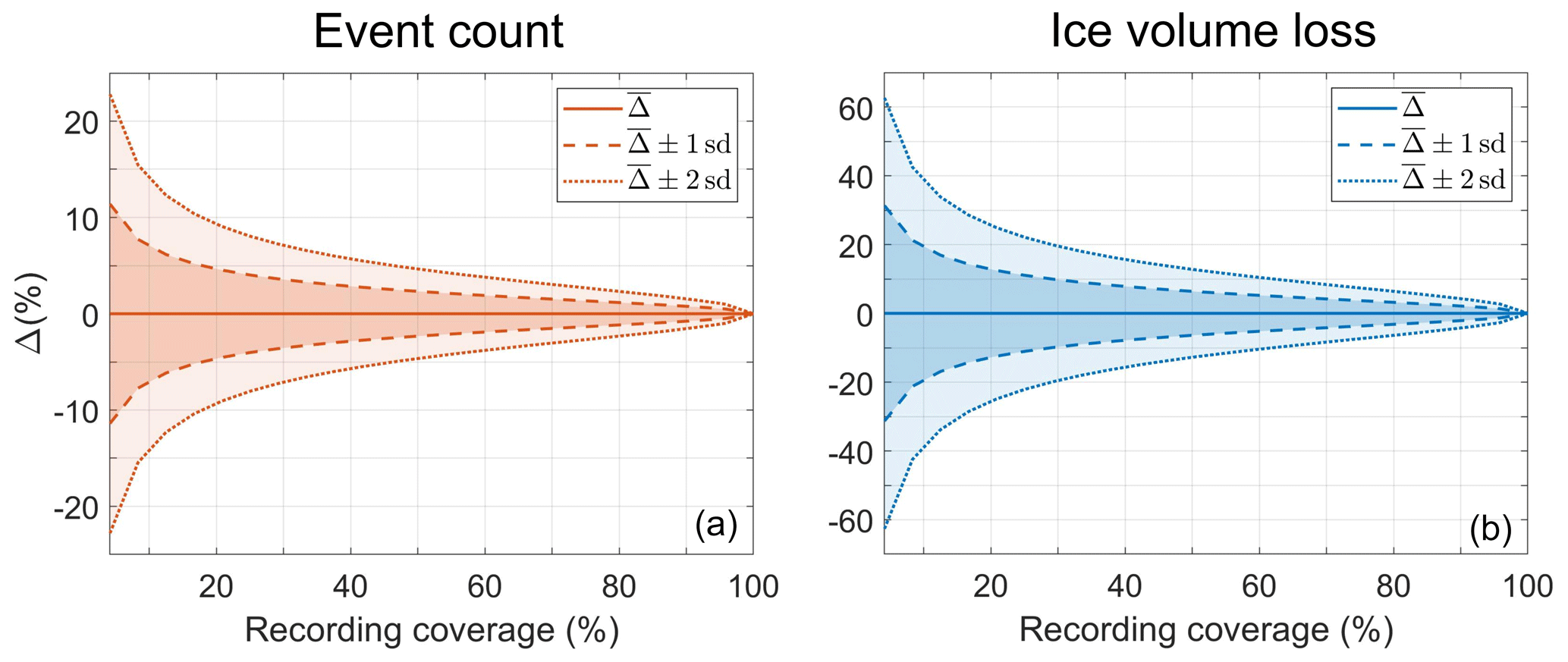
Figure 4The effect of sampling coverage on acoustic estimates of (a) event count and (b) ice volume loss. Recording periods range from 1 h d−1 to continuous. The reference value of Δ=0 % is for full coverage.
Figure 5 shows the percentage of time occupied by calving noise during the experiment and the acoustic estimate of daily calving rate. On average, calving events were active for only about 1 % of the time; this corresponds to around 120 events per day. However, we expect that the calving detector may split single calving events into several detections. This is especially likely in the case of free falls of highly disintegrated icebergs. Therefore, we assume that the real daily calving rate is likely lower than the acoustic estimate. Although calving activity changes significantly with seasons and geographical location, it is still expected to be a small fraction of the total record. Exploiting this fact through the use of event-driven recording systems could result in significant power savings for autonomous recorders.
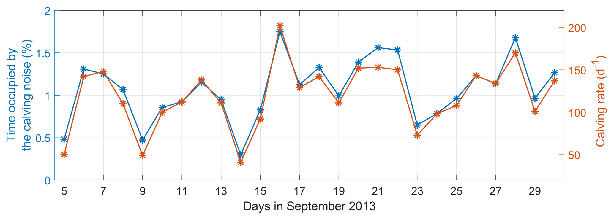
Figure 5(blue) Percentage of time occupied by calving noise over the study period and (orange) the acoustic estimate of daily calving rate.
This first automated analysis of underwater sound recorded near the terminus of a tidewater glacier, compared with camera and satellite observations, demonstrates the feasibility of using cryoacoustics to monitor subaerial calving fluxes over extended periods. Challenges remain. The method has been verified for Hansbreen, a glacier of a scale common to Spitsbergen, but the glaciers in Greenland can be factors of 10 or more larger in both horizontal and vertical scales. Moreover, calving mode and propagation conditions will vary between glaciers, and there will be variability in levels of ice coverage in the terminus bay, which depend on calving rate, circulatory flow (long, narrow fjords are more prone to melange buildup), and sea ice coverage. For example, the detachment of an already floating section of ice from an ice tongue would not necessarily have the same impact on the ocean as a subaerial calving event from a grounded terminus. Some or all of these factors may need to be accounted for when applying cryoacoustics to quantify subaerial calving flux between tidewater glaciers.
Cryoacoustics meets some of the important requirements for long-term monitoring of subaerial calving fluxes. The high rate of signal acquisition ensures that every calving event can be detected, provided its signal is above the detection threshold and below the rejection threshold. Although the uncertainty in the volume estimate for a single event is high, the total volume estimate becomes precise if a sufficient number of events are accumulated (Glowacki and Deane, 2020). With current technological limitations, it is not possible to take time-lapse photographs with high enough frame rates to ensure that all events are captured. Moreover, cryoacoustics is insensitive to lighting conditions and relatively insensitive to weather conditions. For example, the dominant spectral component of noise generated by rain lies well above the “calving band” (Pumphrey and Crum, 1988).
Both cryoacoustics and cryoseismology provide temporally resolved, continuous records of calving activity that are expected to be relatively insensitive to changing environmental conditions (Podolskiy and Walter, 2016; Deane et al., 2019). Cryoacoustics has the additional benefit that the physics of sound production, which stems from the entrainment of bubbles around falling blocks of ice and collective oscillations of bubble plumes (Glowacki, 2020), is expected to apply broadly across calving glaciers in polar regions. If true, this will enable subaerial calving flux to be extracted from cryoacoustic signals without the burden of a glacier-by-glacier calibration. Moreover, it may be possible to extract other geophysical signals of interest, such as terminus melt rate, from cryoacoustic records (Pettit et al., 2015; Deane et al., 2019).
Cryoacoustics, combined with other remote sensing methods, such as photogrammetry, cryoseismology, and satellite observations, can form the core of a long-term monitoring system for subaerial calving fluxes from glaciers and ice shelves.
A1 Acoustic and camera observations
Acoustic and camera data were collected around Hansbreen from 5–30 September 2013. Noise recordings were made with a High Tech. Inc. HTI-96-MIN omnidirectional hydrophone mounted on the seafloor at a depth of 22 m and approximately 1.95 km from the glacier terminus. Data were sampled at a frequency of 32 kHz with 16 bit of dynamic range. Photographs of the terminus were taken every 3 h using a Canon D1000 time-lapse camera located 160 m a.s.l. and 0.8 to 2 km from the glacier terminus (see Fig. 1).
The images were analyzed to estimate the area of ice lost from the cliff face through calving when lighting and weather conditions permitted. Changes at the calving front associated with calving events were found by comparing two consecutive time-lapse images in terms of shape and color of the terminus area. The terminus area loss was then estimated using known ice cliff heights at given locations. This methodology is sensitive to the variability of the terminus shape along its edge due to the oblique angle of the camera view. Moreover, we are aware that the glacier can calve more than once at the same location during a 3 h time frame. Nevertheless, the image analysis provides useful information about the overall calving activity at Hansbreen during the study period.
A2 Satellite observations
The volume of ice lost from Hansbreen through subaerial calving was estimated from satellite imagery and GPS observations of the glacier surface movement. Subaerial calving flux is estimated using , where Q is the volumetric flux of icebergs, is the mean ice flow velocity, Ufront is the front retreat/advance velocity, and L and H respectively are the cliff length and height above sea level. The length of Hansbreen’s active cliff and the average front retreat per day have been extracted from two multispectral Landsat 8 satellite images (24 August 2013 and 25 September 2013). Cliff height above sea level was determined in 2015 using a Riegl VZ-6000 high-resolution 3D laser scanner. Błaszczyk et al. (2021) showed that the average front height has not changed significantly between 1991 and 2015. The glacier surface velocity was estimated using a mass balance stake mounted near the calving front (designated GPS in Fig. A1). Changes in stake positions were measured with dGPS on 6 and 28 August 2013. The initial and final stake coordinates in UTM coordinate system (zone 33N) were 8549150.69 m N, 515877.56 m E and 8549136.03 m N, 515872.57 m E. The average ice velocity was 257 m yr−1. We are aware that these measurements were conducted outside the hydro-acoustic monitoring period. Moreover, a measurement with a single stake is a very rough estimate that does not take into account the variability of glacier velocity along its calving front. However, this is the best approximation available that helps to compare the total ice volume loss estimated from satellite and acoustic data. The subaerial calving flux estimated over the 26 d of acoustic measurements is m3, i.e., ca. 0.27×10⁶ m3 d−1. This is the result used for comparison with the acoustic data. As a crosscheck, the glacier surface velocity field was estimated using offset tracking from TerraSAR satellite radar images (15 December 2012 and 26 December 2012). Subaerial calving flux was then estimated within 40 m sections of the glacier front to allow for variations in velocity and cliff height (see the grey profile in Fig. A1). The total volume of icebergs calved during the observation period is estimated to be m3. It should be borne in mind, however, that satellite images were collected in December 2012 and not during the study period. There is a lack of cloudless multispectral data from 2013 for the area of the Hornsund fiord. Nevertheless, the results show good agreement with subaerial calving flux estimated using stake measurements.
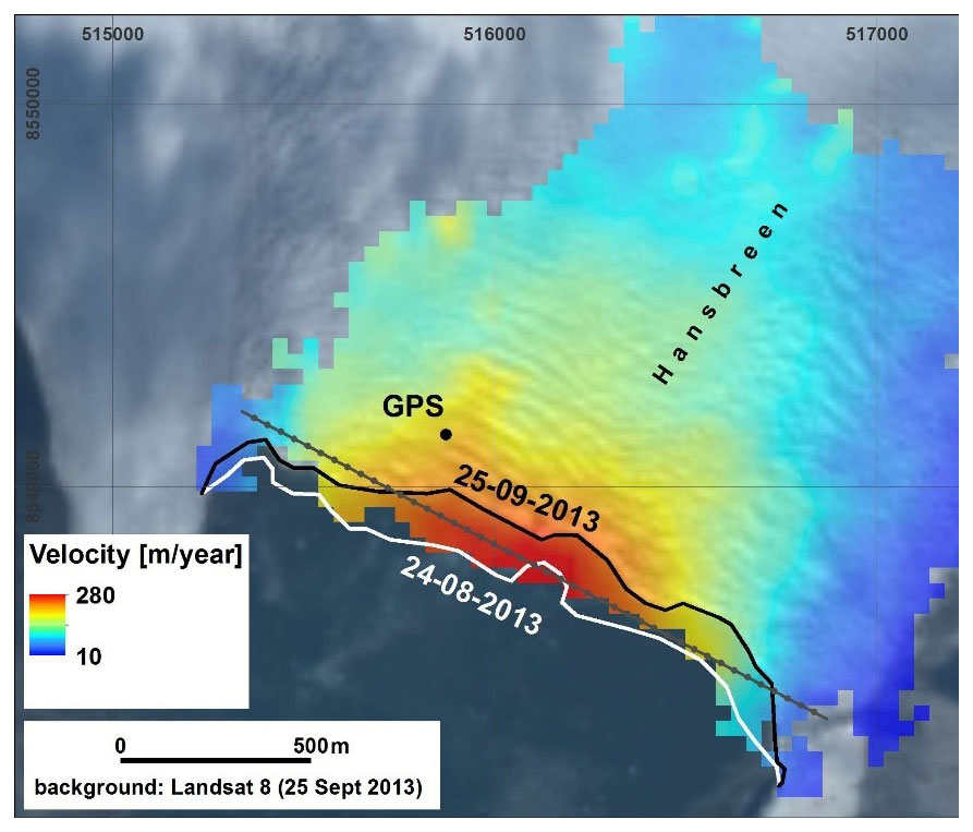
Figure A1Data used in the subaerial calving flux calculations. Horizontal velocity map from offset tracking on repeat TerraSAR satellite radar images (15 December 2012 and 26 December 2012), retreat of Hansbreen cliff between 24 August 2013 and 25 September 2013 and localization of stake position with dGPS measurements. The grey profile with dots shows division of the ice cliff into 40 m lengths, along which precise calculations of subaerial calving flux were made. The map is in UTM projection system (zone 33N).
A3 Calving impact energy estimation
The calving impact energy was estimated from the noise energy using a power-law relationship model shown in Eq. (4). The parameters of the model are based on the calibration dataset presented in Glowacki and Deane (2020) that includes time-lapse images and underwater noise recordings of 169 calving events observed in 2016 at Hansbreen. However, the power-law model proposed by Glowacki and Deane (2020) was improved through the re-analysis of the calibration dataset. The following changes/modifications were applied:
-
Subsequent to publication, it was discovered that the acoustic recordings contained a small DC offset, which created a minor bias in the event energy estimates. This issue has been corrected here by running the acoustic recordings through a (30–100) Hz band-pass filter, the lower frequency of which is roughly equal to the low-frequency cut-off of the waveguide comprised of the sea surface and seafloor of the terminus bay.
-
The Bellhop ray-tracing model was used in Glowacki and Deane (2020) to calculate the loss of acoustic energy between the iceberg/water impact locations and the hydrophone. Here, the transmission loss of the calving noise was calculated using the parabolic equation model RAM (Collins, 1993) that is more recommended for low-frequency problems (Jensen et al., 2011). The grain size of the sediments and source depth were set to ϕ=5 (diameter D=31 µm) and Zs=5 m, respectively. The attenuation, sound speed, and density of the sediments were calculated from the grain size using formulas proposed by Hamilton (1972) and Hamilton and Bachman (1982). Moreover, in the present study, transmission losses were evaluated for a whole range of frequencies between 30 and 100 Hz, while a single nominal source frequency of 50 Hz was used in Glowacki and Deane (2020).
-
In Glowacki and Deane (2020), the parameters of the power-law relationship between the impact energy and noise energy were estimated by performing a linear least-mean-squares analysis of log-transformed variables; the impact noise energy was used as a dependent variable to estimate the impact-to-noise conversion coefficients. Here, the block impact energy was used as a dependent variable to minimize the error in the subaerial calving flux. Moreover, the coefficients of the power-law relationship were estimated using a non-linear regression model and non-transformed variables (function fitnlm in MATLAB).
Problems remain. Most importantly, the calibration dataset is limited to 169 calving events and certainly do not represent the full range of possible values of the impact noise energy at Hansbreen. As a consequence, the power-law model – which is based on the calibration data – certainly requires further improvement. This is confirmed by Fig. A2, which compares histograms and empirical cumulative distribution functions (ECDFs) of Eac,imp computed for acoustic data collected in 2013 (present study) and 2016 (calibration dataset). There are two major conclusions from Fig. A2.
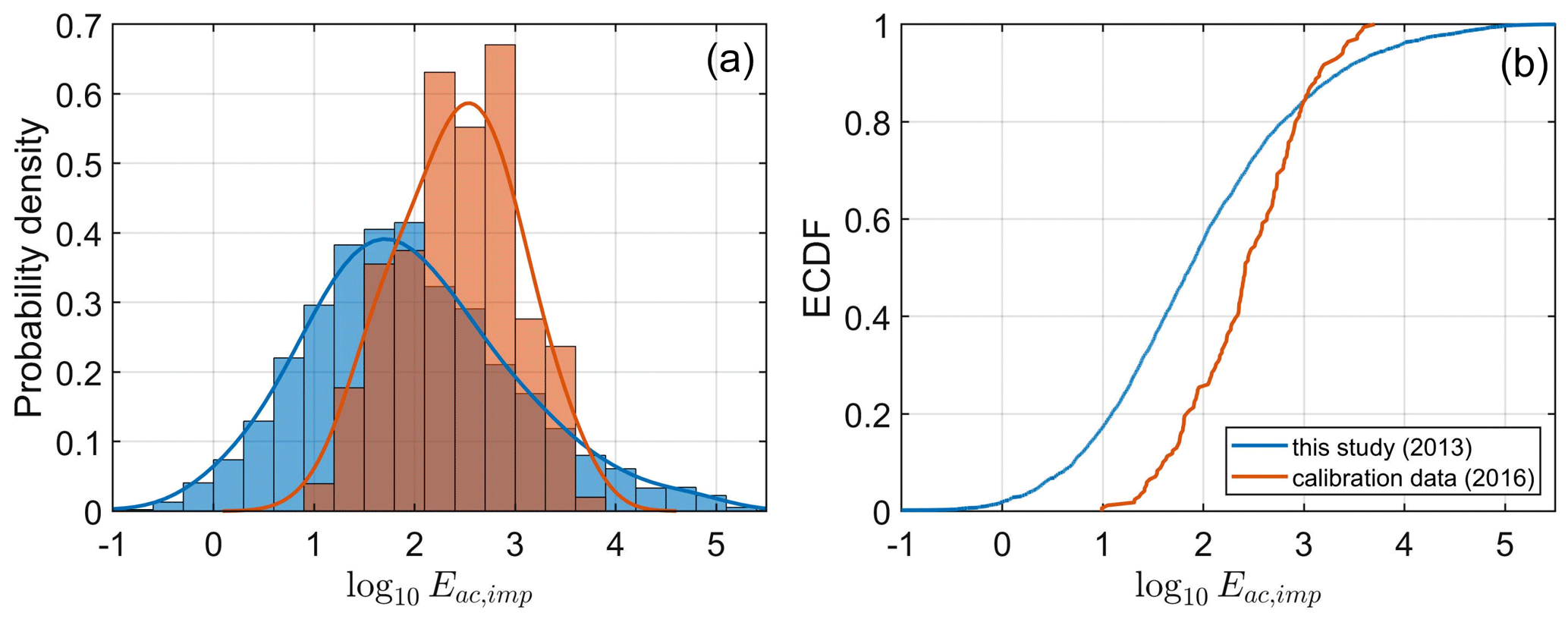
Figure A2(a) Histograms and (b) empirical cumulative distribution functions (ECDFs) of log-transformed impact noise energies calculated for calibration data (2016; orange) and acoustic measurements used in this study (2013; blue).
First, the 2016 data do not include impact noise energies smaller than 10 J. This is to be expected because the calibration dataset requires that all calving events are also captured by the time-lapse camera. Small-scale changes at the glacier terminus were hardly visible on camera images and could not be included in the calibration dataset. Individually, low-magnitude calving events contribute little to the total subaerial calving flux; however, it cannot be ruled out that sometimes they constitute a large fraction of the calving inventory and are meaningful as a whole.
Second, the 2016 data do not include calving events with J either. The lack of the largest events in the calibration dataset may be due to several reasons: (i) Hansbreen may have been in different melting regimes in 2013 and 2016, which caused differences in calving styles (e.g., differences in the water depth at the terminus, glacier surface velocity, water content); (ii) co-occurrence of large-scale calving events and bad weather/lighting conditions that prevented estimation of impact energy from time-lapse images in the calibration dataset; (iii) underestimated transmission loss for the acoustic data collected in 2013 because of the different location of the hydrophone compared to 2016 leading to a different propagation path (note the shallow sill close to the recorder in Fig. 1a). Leaving aside the causes, the lack of the highest-impact noise energies in the calibration dataset results in extrapolation of the power-law model in the analysis of data collected in 2013; unfortunately, the extrapolation applies to calving events that contribute the most to the subaerial calving flux. This is one possible explanation of the discrepancy between calving fluxes derived from traditional methods and the acoustic technique.
The improvement of the power-law model in Eq. (4) requires long-term acoustic measurements close to different glaciers combined with measurements of ice block volumes with optical techniques (e.g., time-lapse photography, terrestrial laser scanning). Collecting calibration data that would include a whole range of styles and magnitudes of calving events is critical for the usefulness of the acoustic technique in the monitoring of subaerial calving fluxes.
A4 Calving event detection algorithm
The calving event detection algorithm depends on the selection of an event detection factor, β, and a frequency band over which the ambient sound is filtered before integration over time.
Figure A3 shows a summary of how the number of detected calving events varies with the detection factor β; interfering events were not removed in this analysis. As might be expected, the total number of events decreases rapidly with increasing detection factor because increasing β results in the exclusion of the lowest-energy events. The results presented in Fig. 3 were generated using β=5, which was found to be an optimal selection in terms of limiting detection of non-calving events and minimizing the loss of true calving events. The selection of β consisted of the visual analysis of noise spectrograms and audible inspection of sound recordings performed for a number of detections.
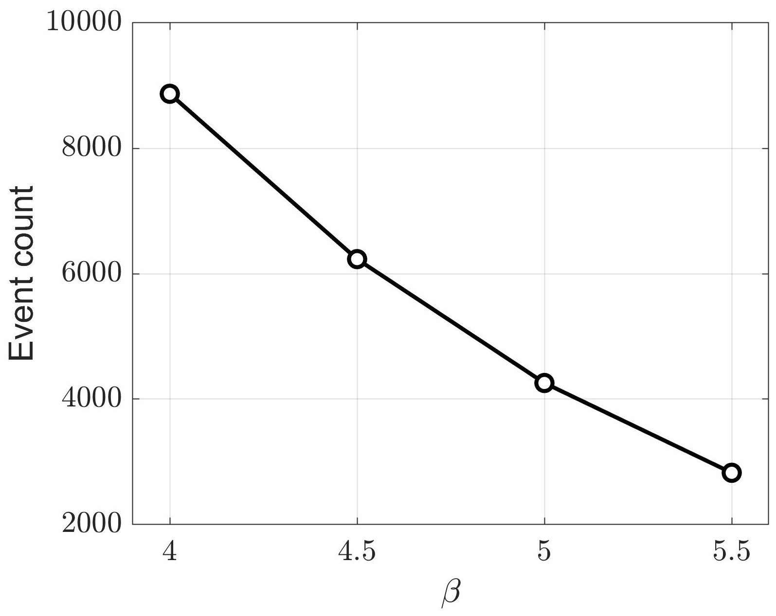
Figure A3Relationship between detection factor β and the number of detected calving events. Interfering events are not removed in this analysis.
The detection factor selected here for the terminal bay of Hansbreen is likely not the optimal detection factor for other environments or geometries for the terminus and recording station. This is because the detector performance is sensitive to the signal-to-noise ratio at the hydrophone location and activity of other sources, such as nearby icebergs, which will vary from site to site.
It is noted in the main text that the event detection algorithm is based on the assumption that a good estimate for the background noise is the median noise level in the detector frequency band. This assumption holds well when calving events are relatively infrequent within an observational interval selected for analysis (10 min here) but may bias the detector toward the exclusion of low-energy events if too many events occur within the interval. The validity of the assumption was tested by computing the background noise level iteratively: detected events are removed from the record and a baseline noise level recomputed in successive passes through the data segment. The results of this analysis for change in number of events detected, total acoustic energy at the receiver, and summed event durations are shown in Fig. A4. The total percentage change in acoustic energy of all detected events is less than 3 %, which is not a significant source of error given other, larger uncertainties in the analysis, such as hydrophone calibration and propagation loss. The percentage change in number of events is similarly minor. There is a larger impact on the duration of events because of two effects: (1) increasing the baseline noise level increases the detection threshold and decreases event duration, and (2) the division of a single event into two or more events is sensitive to the baseline noise level.
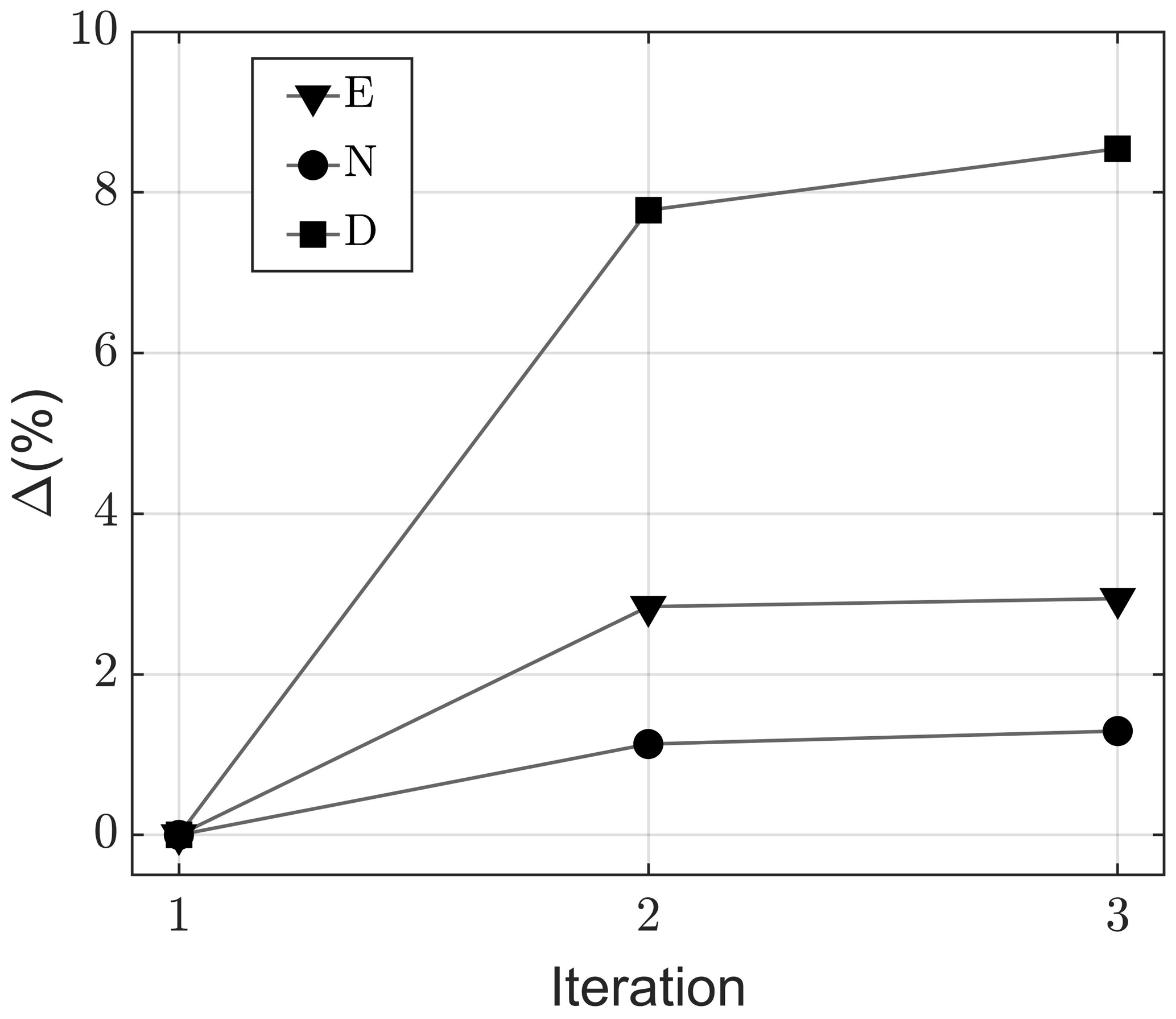
Figure A4Change in number of events detected (N), total acoustic energy at the receiver (E), and summed event durations (D) versus iteration number for the background noise estimate.
Here we use a simple but robust algorithm for the detection of subaerial calving events. The calving detector in the present form has two major weaknesses: (1) subaerial and submarine calving events cannot be distinguished and treated separately, and (2) certainly there are still some unexplored interfering events that either cause false detections or periodically lower the signal-to-noise ratio, which makes calving detection more difficult (i.e., some calving events remain undetected). The latter issue can be partly addressed with the use of more sophisticated detection techniques. See, for example, recent work in the cryoseismology community by Carr et al. (2020) and Köhler et al. (2022). However, we speculate that better understanding of different (non-calving) sound-source mechanisms and their underwater acoustic signatures is required before more sophisticated algorithms are implemented. Examples may include but are not limited to interactions between floating growlers and icebergs, ice fracturing events, water outflows from subglacial conduits, coastline landslides, and activity of marine mammals. Most of these “interfering” noise sources can be investigated with meteorological and oceanographic measurements, high-frequency photographic images, laser scans, or radar scans synchronized with acoustic recordings. For example, Deane et al. (2014) reported that interactions of surface gravity waves with underside of ice ledges at the periphery of icebergs are sources of underwater noise emission below 500 Hz. Some sound-source mechanisms, like underwater fracturing events, require novel observational techniques or scaled laboratory experiments.
The problem remains with detection of submarine events. An inclusion of submarine events would be beneficial for two reasons: (i) to find out how frequent these events are and (ii) to provide more accurate estimates of subaerial calving fluxes by rejecting submarine events from the analysis. Moreover, it should not be ruled out that the methodology for estimating submarine calving fluxes from sound recordings made in glacial bays could be developed. If so, it would be possible to derive both subaerial and submarine calving fluxes using acoustic techniques. Recent work by Glowacki (2022) demonstrated that the two calving modes can be acoustically distinguished using parameters of the log-normal distribution of the calving noise combined with calving signal duration. A semi-automatic detection of start and end times of calving noise was used. However, the problem remains of how to automatically select t0 and t1 for submarine calving events; this would require a long-term calibration dataset of synchronized high-frequency time-lapse images and noise recordings. Such data are not available for calving events observed in 2013. Consequently, the analysis of submarine events was out of the scope of this study.
The acoustic data used in this study are available at https://doi.org/10.34808/jp25-2b47 (Tegowski et al., 2023). Time-lapse images of the Hansbreen's terminus can be downloaded from https://ppdb.us.edu.pl/geonetwork/srv/eng/catalog.search#/metadata/ee0e611b-bfe9-4ba1-95ae-beb0702ae2aa (Ciepły, 2023). CTD data – used for noise propagation modeling – are available at https://dataportal.igf.edu.pl/dataset/inter-calibrated-temperature-and-salinity-in-depth-profiles-in-hornsund-fjord (Moskalik et al., 2022).
JT conceived the project, led the 2013 field expedition to Svalbard and participated in data analysis and interpretation, and participated in manuscript preparation. OG is co-architect of the sound inversion methodology, performed data analysis and interpretation, and participated in manuscript preparation. MC collected and processed the photographic data of terminus ablation. MB collected and processed satellite and stick data of glacier velocity and ice mass loss. JJ provided scientific oversight into data analysis and participated in manuscript preparation. MM participated in the field campaigns and provided CTD data. PB participated in field campaigns and participated in manuscript preparation. GBD is co-architect of the sound inversion methodology and detection algorithm, participated in field campaign, and participated in manuscript preparation.
The contact author has declared that none of the authors has any competing interests.
Publisher’s note: Copernicus Publications remains neutral with regard to jurisdictional claims in published maps and institutional affiliations.
We gratefully acknowledge the support of the staff at the Stanisław Siedlecki Polish Polar Research Station in Hornsund (PPS). TerraSAR-X data were provided by German Aerospace Center (DLR, project LAN2787). Landsat-8 data were made available by the United States Geological Survey (USGS). We thank Evgeny Podolskiy, the anonymous reviewer, and the handling editor, Olaf Eisen, for their insightful comments.
This research has been supported by the Ministry of Education and Science, Poland (subsidy for the Institute of Geophysics, Polish Academy of Sciences, and grant no. 1621/MOB/V/2017/0), the National Science Centre, Poland (grant nos. 2021/43/D/ST10/00616 and 2011/03/B/ST10/04275), the Centre for Polar Studies, University of Silesia, the U.S. Office of Naval Research, Ocean Acoustics Division (grant no. N00014-17-1-2633), the U.S. National Science Foundation Office of Polar Programs (grant no. OPP-1748265), and Research Council of Norway (Arctic Field Grant, RIS ID: 6133).
This paper was edited by Olaf Eisen and reviewed by Evgeny A. Podolskiy and one anonymous referee.
Benn, D. I., Hulton, N. R., and Mottram, R. H.: “Calving laws”, “sliding laws” and the stability of tidewater glaciers, Ann. Glaciol., 46, 123–130, https://doi.org/10.3189/172756407782871161, 2007a. a
Benn, D. I., Warren, C. R., and Mottram, R. H.: Calving processes and the dynamics of calving glaciers, Earth-Sci. Rev., 82, 143–179, https://doi.org/10.1016/j.earscirev.2007.02.002, 2007b. a, b
Błaszczyk, M., Jania, J. A., and Hagen, J. O.: Tidewater glaciers of Svalbard: Recent changes and estimates of calving fluxes, Pol. Polar Res., 30, 85–142, 2009. a
Błaszczyk, M., Jania, J. A., and Kolondra, L.: Fluctuations of tidewater glaciers in Hornsund Fjord (Southern Svalbard) since the beginning of the 20th century, Pol. Polar Res., 34, 327–352, https://journals.pan.pl/dlibra/publication/114504/edition/99557/content (last access: 16 October 2023), 2013. a
Błaszczyk, M., Ignatiuk, D., Uszczyk, A., Cielecka-Nowak, K., Grabiec, M., Jania, J. A., Moskalik, M., and Walczowski, W.: Freshwater input to the Arctic fjord Hornsund (Svalbard), Polar Res., 38, 3506, https://doi.org/10.33265/polar.v38.3506, 2019. a
Błaszczyk, M., Jania, J. A., Ciepły, M., Grabiec, M., Ignatiuk, D., Kolondra, L., Kruss, A., Luks, B., Moskalik, M., Pastusiak, T., Strzelewicz, A., Walczowski, W., and Wawrzyniak, T.: Factors Controlling Terminus Position of Hansbreen, a Tidewater Glacier in Svalbard, J. Geophys. Res.-Earth, 126, e2020JF005763, https://doi.org/10.1029/2020JF005763, 2021. a, b, c, d
Carr, C. G., Carmichael, J. D., Pettit, E. C., and Truffer, M.: The influence of environmental microseismicity on detection and interpretation of small-magnitude events in a polar glacier setting, J. Glaciol., 66, 790–806, https://doi.org/10.1017/jog.2020.48, 2020. a
Ciepły, M.: Time-lapse images of Hansbreen frontal zone (05–30.09.2013), Polish Polar Data Base [data set], https://ppdb.us.edu.pl/geonetwork/srv/eng/catalog.search#/metadata/ee0e611b-bfe9-4ba1-95ae-beb0702ae2aa, last access: 16 October 2023. a
Collins, M. D.: A split‐step Padé solution for the parabolic equation method, J. Acoust. Soc. Am., 93, 1736–1742, https://doi.org/10.1121/1.406739, 1993. a, b
Deane, G. B., Glowacki, O., Tegowski, J., Moskalik, M., and Blondel, P.: Directionality of the ambient noise field in an Arctic, glacial bay, J. Acoust. Soc. Am., 136, EL350–EL356, https://doi.org/10.1121/1.4897354, 2014. a, b
Deane, G. B., Glowacki, O., Dale Stokes, M., and Pettit, E.: The Underwater Sounds of Glaciers, Acoustics Today, 15, 12–19, https://doi.org/10.1121/AT.2019.15.4.12, 2019. a, b, c
DeConto, R. M., Pollard, D., Alley, R. B., Velicogna, I., Gasson, E., Gomez, N., Sadai, S., Condron, A., Gilford, D. M., Ashe, E. L., Kopp, R. E., Li, D., and Dutton, A.: The Paris Climate Agreement and future sea-level rise from Antarctica, Nature, 593, 83–89, https://doi.org/10.1038/s41586-021-03427-0, 2021. a
Glowacki, O.: Underwater noise from glacier calving: Field observations and pool experiment, J. Acoust. Soc. Am., 148, EL1–EL7, https://doi.org/10.1121/10.0001494, 2020. a, b
Glowacki, O.: Distinguishing subaerial and submarine calving with underwater noise, J. Glaciol., 68, 1185–1196, https://doi.org/10.1017/jog.2022.32, 2022. a, b, c, d, e, f
Glowacki, O. and Deane, G. B.: Quantifying iceberg calving fluxes with underwater noise, The Cryosphere, 14, 1025–1042, https://doi.org/10.5194/tc-14-1025-2020, 2020. a, b, c, d, e, f, g, h, i, j, k, l, m, n, o, p, q, r
Glowacki, O., Deane, G. B., Moskalik, M., Blondel, P., Tegowski, J., and Blaszczyk, M.: Underwater acoustic signatures of glacier calving, Geophys. Res. Lett., 42, 804–812, https://doi.org/10.1002/2014GL062859, 2015. a
Glowacki, O., Moskalik, M., and Deane, G. B.: The impact of glacier meltwater on the underwater noise field in a glacial bay, J. Geophys. Res.-Oceans, 121, 8455–8470, https://doi.org/10.1002/2016JC012355, 2016. a
Glowacki, O., Deane, G. B., and Moskalik, M.: The Intensity, Directionality, and Statistics of Underwater Noise From Melting Icebergs, Geophys. Res. Lett., 45, 4105–4113, https://doi.org/10.1029/2018GL077632, 2018. a
Hamilton, E. L.: Compressional-wave attenuation in marine sediments, Geophysics, 37, 620–646, https://doi.org/10.1190/1.1440287, 1972. a
Hamilton, E. L. and Bachman, R. T.: Sound velocity and related properties of marine sediments, J. Acoust. Soc. Am., 72, 1891–1904, https://doi.org/10.1121/1.388539, 1982. a
How, P., Schild, K. M., Benn, D. I., Noormets, R., Kirchner, N., Luckman, A., Vallot, D., Hulton, N. R. J., and Borstad, C.: Calving controlled by melt-under-cutting: detailed calving styles revealed through time-lapse observations, Ann. Glaciol., 60, 20–31, https://doi.org/10.1017/aog.2018.28, 2019. a, b
Intergovernmental Panel on Climate Change (IPCC): Climate Change 2021 – The Physical Science Basis: Working Group I Contribution to the Sixth Assessment Report of the Intergovernmental Panel on Climate Change, Cambridge University Press, Cambridge, United Kingdom and New York, NY, USA, https://doi.org/10.1017/9781009157896, 2023. a, b
Jensen, F. B., Kuperman, W. A., Porter, M. B., and Schmidt, H.: Computational Ocean Acoustics, 2nd edn., Springer Publishing Company, Incorporated, https://doi.org/10.1007/978-1-4419-8678-8, 2011. a
Köhler, A., Nuth, C., Kohler, J., Berthier, E., Weidle, C., and Schweitzer, J.: A 15 year record of frontal glacier ablation rates estimated from seismic data, Geophys. Res. Lett., 43, 12155–12164, https://doi.org/10.1002/2016GL070589, 2016. a
Köhler, A., Pętlicki, M., Lefeuvre, P.-M., Buscaino, G., Nuth, C., and Weidle, C.: Contribution of calving to frontal ablation quantified from seismic and hydroacoustic observations calibrated with lidar volume measurements, The Cryosphere, 13, 3117–3137, https://doi.org/10.5194/tc-13-3117-2019, 2019. a
Köhler, A., Myklebust, E. B., and Mæland, S.: Enhancing seismic calving event identification in Svalbard through empirical matched field processing and machine learning, Geophys. J. Int., 230, 1305–1317, https://doi.org/10.1093/gji/ggac117, 2022. a
Luckman, A., Benn, D. I., Cottier, F., Bevan, S., Nilsen, F., and Inall, M.: Calving rates at tidewater glaciers vary strongly with ocean temperature, Nat. Commun., 6, 8566, https://doi.org/10.1038/ncomms9566, 2015. a
Medrzycka, D., Benn, D. I., Box, J. E., Copland, L., and Balog, J.: Calving Behavior at Rink Isbræ, West Greenland, from Time-Lapse Photos, Arct. Antarct. Alp. Res., 48, 263–277, https://doi.org/10.1657/AAAR0015-059, 2016. a
Meredith, M. P., Inall, M. E., Brearley, J. A., Ehmen, T., Sheen, K., Munday, D., Cook, A., Retallick, K., Landeghem, K. V., Gerrish, L., Annett, A., Carvalho, F., Jones, R., Garabato, A. C. N., Bull, C. Y. S., Wallis, B. J., Hogg, A. E., and Scourse, J.: Internal tsunamigenesis and ocean mixing driven by glacier calving in Antarctica, Science Advances, 8, eadd0720, https://doi.org/10.1126/sciadv.add0720, 2022. a
Minowa, M., Podolskiy, E. A., Sugiyama, S., Sakakibara, D., and Skvarca, P.: Glacier calving observed with time-lapse imagery and tsunami waves at Glaciar Perito Moreno, Patagonia, J. Glaciol., 64, 362–376, https://doi.org/10.1017/jog.2018.28, 2018. a
Moskalik, M., Ćwiąkała, J., Szczuciński, W., Dominiczak, A., Głowacki, O., Wojtysiak, K., and Zagórski, P.: Spatiotemporal changes in the concentration and composition of suspended particulate matter in front of Hansbreen, a tidewater glacier in Svalbard, Oceanologia, 60, 446–463, https://doi.org/10.1016/j.oceano.2018.03.001, 2018. a, b
Moskalik, M., Głowacki, O., and Korhonen, M.: Inter-calibrated Temperature and Salinity in-depth profiles in Hornsund Fjord, IG PAS Data Portal [data set], https://dataportal.igf.edu.pl/dataset/inter-calibrated-temperature-and-salinity-in-depth-profiles-in-hornsund-fjord, 2022. a
Motyka, R.: Deep-water calving at Le Conte Glacier, Southeast Alaska, in: Calving Glaciers: Report of a Workshop, 28 February–2 March 1997, BPRC Report No. 15, edited by: van der Veen, C., Byrd Polar Research Center, The Ohio State University, Columbus, Ohio, 115–118, https://kb.osu.edu/bitstream/handle/1811/44487/BPRC_Report_15_Part2.pdf (last access: 16 October 2023), 1997. a
Mouginot, J., Rignot, E., Bjørk, A. A., van den Broeke, M., Millan, R., Morlighem, M., Noël, B., Scheuchl, B., and Wood, M.: Forty-six years of Greenland Ice Sheet mass balance from 1972 to 2018, P. Natl. Acad. Sci., 116, 9239–9244, https://doi.org/10.1073/pnas.1904242116, 2019. a
Noël, B., van Kampenhout, L., Lenaerts, J. T. M., van de Berg, W. J., and van den Broeke, M. R.: A 21st Century Warming Threshold for Sustained Greenland Ice Sheet Mass Loss, Geophys. Res. Lett., 48, e2020GL090471, https://doi.org/10.1029/2020GL090471, 2021. a
Nolan, J. P.: Univariate Stable Distributions – Models for Heavy Tailed Data, Springer, Cham, Switzerland, https://doi.org/10.1007/978-3-030-52915-4, 2021. a
Nystuen, J. A.: Rainfall measurements using underwater ambient noise, J. Acoust. Soc. Am., 79, 972–982, https://doi.org/10.1121/1.393695, 1986. a
O'Neel, S., Marshall, H. P., McNamara, D. E., and Pfeffer, W. T.: Seismic detection and analysis of icequakes at Columbia Glacier, Alaska, J. Geophys. Res.-Earth, 112, F03S23, https://doi.org/10.1029/2006JF000595, 2007. a
Paolo, F. S., Fricker, H. A., and Padman, L.: Volume loss from Antarctic ice shelves is accelerating, Science, 348, 327–331, https://doi.org/10.1126/science.aaa0940, 2015. a
Pattyn, F. and Morlighem, M.: The uncertain future of the Antarctic Ice Sheet, Science, 367, 1331–1335, https://doi.org/10.1126/science.aaz5487, 2020. a
Pattyn, F., Ritz, C., Hanna, E., Asay-Davis, X., DeConto, R., Durand, G., Favier, L., Fettweis, X., Goelzer, H., Golledge, N. R., Kuipers Munneke, P., Lenaerts, J. T. M., Nowicki, S., Payne, A. J., Robinson, A., Seroussi, H., Trusel, L. D., and van den Broeke, M.: The Greenland and Antarctic ice sheets under 1.5 °C global warming, Nat. Clim. Change, 8, 1053–1061, https://doi.org/10.1038/s41558-018-0305-8, 2018. a
Pętlicki, M. and Kinnard, C.: Calving of Fuerza Aérea Glacier (Greenwich Island, Antarctica) observed with terrestrial laser scanning and continuous video monitoring, J. Glaciol., 62, 835–846, https://doi.org/10.1017/jog.2016.72, 2016. a
Pętlicki, M., Ciepły, M., Jania, J. A., Promińska, A., and Kinnard, C.: Calving of a tidewater glacier driven by melting at the waterline, J. Glaciol., 61, 851–863, https://doi.org/10.3189/2015JoG15J062, 2015. a, b
Pettit, E. C., Lee, K. M., Brann, J. P., Nystuen, J. A., Wilson, P. S., and O'Neel, S.: Unusually loud ambient noise in tidewater glacier fjords: A signal of ice melt, Geophys. Res. Lett., 42, 2309–2316, https://doi.org/10.1002/2014GL062950, 2015. a, b, c
Podgórski, J. and Pętlicki, M.: Detailed Lacustrine Calving Iceberg Inventory from Very High Resolution Optical Imagery and Object-Based Image Analysis, Remote Sensing, 12, 1807, https://doi.org/10.3390/rs12111807, 2020. a
Podgórski, J., Pętlicki, M., and Kinnard, C.: Revealing recent calving activity of a tidewater glacier with terrestrial LiDAR reflection intensity, Cold Reg. Sci. Technol., 151, 288–301, https://doi.org/10.1016/j.coldregions.2018.03.003, 2018. a
Podolskiy, E. A. and Walter, F.: Cryoseismology, Rev. Geophys., 54, 708–758, https://doi.org/10.1002/2016RG000526, 2016. a, b
Podolskiy, E. A., Murai, Y., Kanna, N., and Sugiyama, S.: Glacial earthquake-generating iceberg calving in a narwhal summering ground: The loudest underwater sound in the Arctic?, J. Acoust. Soc. Am., 151, 6–16, https://doi.org/10.1121/10.0009166, 2022. a
Pumphrey, H. C. and Crum, L. A.: Acoustic Emissions Associated with Drop Impacts, in: Sea Surface Sound: Natural Mechanisms of Surface Generated Noise in the Ocean, edited by: Kerman, B. R., Springer Netherlands, Dordrecht, 463–483, https://doi.org/10.1007/978-94-009-3017-9_34, 1988. a
Schellenberger, T., Dunse, T., Kääb, A., Kohler, J., and Reijmer, C. H.: Surface speed and frontal ablation of Kronebreen and Kongsbreen, NW Svalbard, from SAR offset tracking, The Cryosphere, 9, 2339–2355, https://doi.org/10.5194/tc-9-2339-2015, 2015. a
Smith, B., Fricker, H. A., Gardner, A. S., Medley, B., Nilsson, J., Paolo, F. S., Holschuh, N., Adusumilli, S., Brunt, K., Csatho, B., Harbeck, K., Markus, T., Neumann, T., Siegfried, M. R., and Zwally, H. J.: Pervasive ice sheet mass loss reflects competing ocean and atmosphere processes, Science, 368, 1239–1242, https://doi.org/10.1126/science.aaz5845, 2020. a
Straneo, F., Heimbach, P., Sergienko, O., Hamilton, G., Catania, G., Griffies, S., Hallberg, R., Jenkins, A., Joughin, I., Motyka, R., Pfeffer, W. T., Price, S. F., Rignot, E., Scambos, T., Truffer, M., and Vieli, A.: Challenges to Understanding the Dynamic Response of Greenland's Marine Terminating Glaciers to Oceanic and Atmospheric Forcing, B. Am. Meteorol. Soc., 94, 1131–1144, https://doi.org/10.1175/BAMS-D-12-00100.1, 2013. a
Straneo, F., Sutherland, D. A., Stearns, L., Catania, G., Heimbach, P., Moon, T., Cape, M. R., Laidre, K. L., Barber, D., Rysgaard, S., Mottram, R., Olsen, S., Hopwood, M. J., and Meire, L.: The Case for a Sustained Greenland Ice Sheet-Ocean Observing System (GrIOOS), Frontiers in Marine Science, 6, 138, https://doi.org/10.3389/fmars.2019.00138, 2019. a
Sugiyama, S., Minowa, M., and Schaefer, M.: Underwater Ice Terrace Observed at the Front of Glaciar Grey, a Freshwater Calving Glacier in Patagonia, Geophys. Res. Lett., 46, 2602–2609, https://doi.org/10.1029/2018GL081441, 2019. a
Sutherland, D. A., Jackson, R. H., Kienholz, C., Amundson, J. M., Dryer, W. P., Duncan, D., Eidam, E. F., Motyka, R. J., and Nash, J. D.: Direct observations of submarine melt and subsurface geometry at a tidewater glacier, Science, 365, 369–374, https://doi.org/10.1126/science.aax3528, 2019. a
Tegowski, J., Glowacki, O., Ciepły, M., Błaszczyk, M., Jania, J., Moskalik, M., Blondel, P., and Deane, G.: Underwater noise recorded in Hornsund Fjord, Spitsbergen, at the front of the Hans Glacier, Most Wiedzy – Gdańsk University of Technology [data set], https://doi.org/10.34808/jp25-2b47, 2023. a
Truffer, M. and Motyka, R. J.: Where glaciers meet water: Subaqueous melt and its relevance to glaciers in various settings, Rev. Geophys., 54, 220–239, https://doi.org/10.1002/2015RG000494, 2016. a
Urick, R. J.: The Noise of Melting Icebergs, J. Acoust. Soc. Am., 50, 337–341, https://doi.org/10.1121/1.1912637, 1971. a
Vagle, S., Large, W. G., and Farmer, D. M.: An Evaluation of the WOTAN Technique of Inferring Oceanic Winds from Underwater Ambient Sound, J. Atmos. Ocean. Tech., 7, 576–595, https://doi.org/10.1175/1520-0426(1990)007<0576:AEOTWT>2.0.CO;2, 1990. a
van der Veen, C. J.: Calving glaciers, Prog. Phys. Geog., 26, 96–122, https://doi.org/10.1191/0309133302pp327ra, 2002. a, b
Vieli, A., Jania, J., Blatter, H., and Funk, M.: Short-term velocity variations on Hansbreen, a tidewater glacier in Spitsbergen, J. Glaciol., 50, 389–398, https://doi.org/10.3189/172756504781829963, 2004. a
Walter, A., Lüthi, M. P., and Vieli, A.: Calving event size measurements and statistics of Eqip Sermia, Greenland, from terrestrial radar interferometry, The Cryosphere, 14, 1051–1066, https://doi.org/10.5194/tc-14-1051-2020, 2020. a
Warren, C. R., Glasser, N. F., Harrison, S., Winchester, V., Kerr, A. R., and Rivera, A.: Characteristics of tide-water calving at Glaciar San Rafael, Chile, J. Glaciol., 41, 273–289, https://doi.org/10.3189/S0022143000016178, 1995. a
Xie, S., Dixon, T. H., Voytenko, D., Deng, F., and Holland, D. M.: Grounding line migration through the calving season at Jakobshavn Isbræ, Greenland, observed with terrestrial radar interferometry, The Cryosphere, 12, 1387–1400, https://doi.org/10.5194/tc-12-1387-2018, 2018. a
Yun, S., Lee, W. S., Dziak, R. P., Roche, L., Matsumoto, H., Lau, T.-K., Sremba, A., Mellinger, D. K., Haxel, J. H., Kang, S.-G., Hong, J. K., and Park, Y.: Quantifying Soundscapes in the Ross Sea, Antarctica Using Long-Term Autonomous Hydroacoustic Monitoring Systems, Frontiers in Marine Science, 8, 703411, https://doi.org/10.3389/fmars.2021.703411, 2021. a
- Abstract
- Introduction
- Study site
- Automatic detection of calving events
- Interfering event removal
- Estimating ice volume loss
- Results
- Long-term monitoring of subaerial calving fluxes
- Concluding remarks
- Appendix A: Materials and methods
- Data availability
- Author contributions
- Competing interests
- Disclaimer
- Acknowledgements
- Financial support
- Review statement
- References