the Creative Commons Attribution 4.0 License.
the Creative Commons Attribution 4.0 License.
 | 20 Jan 2023
Inter-comparison and evaluation of Arctic sea ice type products
Yufang Ye
Yanbing Luo
Mohammed Shokr
Signe Aaboe
Fanny Girard-Ardhuin
Fengming Hui
Xiao Cheng
Zhuoqi Chen
Arctic sea ice type (SITY) variation is a sensitive indicator of climate change. However, systematic inter-comparison and analysis for SITY products are lacking. This study analysed eight daily SITY products from five retrieval approaches covering the winters of 1999–2019, including purely radiometer-based (C3S-SITY), scatterometer-based (KNMI-SITY and IFREMER-SITY) and combined ones (OSISAF-SITY and Zhang-SITY). These SITY products were inter-compared against a weekly sea ice age product (i.e. NSIDC-SIA – National Snow and Ice Data Center sea ice age) and evaluated with five synthetic aperture radar (SAR) images. The average Arctic multiyear ice (MYI) extent difference between the SITY products and NSIDC-SIA varies from to 0.49×10⁶ km2. Among them, KNMI-SITY and Zhang-SITY in the QuikSCAT (QSCAT) period (2002–2009) agree best with NSIDC-SIA and perform the best, with the smallest bias of km2 in first-year ice (FYI) extent and km2 in MYI extent. In the Advanced Scatterometer (ASCAT) period (2007–2019), KNMI-SITY tends to overestimate MYI (especially in early winter), whereas Zhang-SITY and IFREMER-SITY tend to underestimate MYI. C3S-SITY performs well in some early winter cases but exhibits large temporal variabilities like OSISAF-SITY. Factors that could impact performances of the SITY products are analysed and summarized. (1) The Ku-band scatterometer generally performs better than the C-band scatterometer for SITY discrimination, while the latter sometimes identifies FYI more accurately, especially when surface scattering dominates the backscatter signature. (2) A simple combination of scatterometer and radiometer data is not always beneficial without further rules of priority. (3) The representativeness of training data and efficiency of classification are crucial for SITY classification. Spatial and temporal variation in characteristic training datasets should be well accounted for in the SITY method. (4) Post-processing corrections play important roles and should be considered with caution.


Sea ice is an important component of the earth system. Sea ice influences climate change through two primary processes: the ice–albedo feedback and the insulating effect. Sea ice reflects more solar radiation than the ocean due to its high albedo. In addition, sea ice hinders the heat exchange between the ocean and the atmosphere because of its low thermal conductivity. Through global warming, the loss of sea ice leads to increased absorption of solar radiation and heat flux from the ocean to the atmosphere, which further enhances the loss of sea ice and global warming. Arctic sea ice has been declining dramatically over the past 4 decades (Onarheim et al., 2018; Comiso et al., 2008). Its extent has reduced by 40 %–50 % compared to its average in the 1980s (Perovich et al., 2020), whereas the average ice thickness has decreased by about 1.75 m in winter in the central Arctic Ocean (Rothrock et al., 2008; Kwok and Cunningham, 2015), which has eventually led to a volume loss of roughly 66 % since 1980 (Petty et al., 2020; Kwok, 2018). Meanwhile, the ice drifting and deformation rates are increasing (Kwok et al., 2013; Hakkinen et al., 2008). The Arctic sea ice has been increasingly dominated by thinner and younger first-year ice (FYI) instead of thicker and older multiyear ice (MYI), the ice that has survived at least one summer melt (Maslanik et al., 2007; Tschudi et al., 2020). FYI comprised 35 %–50 % of the ice cover in the mid-1980s. In comparison, this proportion increased to about 70 % in 2019, while MYI covered less than one-third of the Arctic Ocean (Perovich et al., 2021; Kwok, 2018). The change in sea ice type (SITY) distribution impacts the climate of the Arctic and mid- to high-latitude regions through changes in water vapour, cloud properties and large-scale atmospheric circulations (Liu et al., 2012; Screen et al., 2013; Belter et al., 2021; Boisvert et al., 2015). In addition, it influences the Arctic ecosystems by changing the habitat conditions for various Arctic species and is crucial for human activities such as shipping, tourism and resource extraction (Emmerson and Lahn, 2012; Meier et al., 2014). Studies found that the MYI area anomalies can largely explain (about 85 %) the variance in Arctic sea ice volume anomalies (Kwok, 2018). Understanding the distribution and transition of Arctic SITY (especially MYI) is therefore of great scientific and practical importance. SITY is a key parameter for sea ice thickness and total ice volume estimation (Alexandrov et al., 2010). The incorrect assignment of SITY of a grid cell can distort the corresponding calculated ice thickness by more than 25 % (Kwok and Cunningham, 2015). Accurate estimation of SITY is needed in many other areas of interest, e.g. ice navigation, off-shore engineering and construction (IMarEST, 2015) and weather forecasting (Jung et al., 2014).
To monitor Arctic sea ice type distribution changes at the hemispheric scale, various algorithms have been developed using microwave satellite data. Among them, most algorithms focus on the discrimination of MYI and FYI. These algorithms identify SITY (i.e. the discrimination of MYI and FYI in this study) based on the distinct radiometric and scattering characteristics of different ice types. On the one hand, brightness temperatures (Tbs) of MYI tend to be lower than those of FYI because of its low-loss, low-salinity properties (Vant et al., 1978; Weeks and Ackley, 1986). Such a difference is generally larger at higher frequencies (i.e. smaller penetration depth), which reflects the distinguished physical properties of MYI and FYI at the sub-surface layer (Shokr and Sinha, 2015). On the other hand, due to the high volume scattering and low scattering loss, MYI has a relatively higher backscatter than FYI at the same frequency (Onstott, 1992). Note that MYI and FYI have such different microwave characteristics in winter but not in summer or during melt events when snow is wet, which leads to similar microwave signatures of the different ice types. There exist different algorithms which provide either a fractional MYI–FYI coverage or assignment of one or the other ice type (e.g. MYI and FYI) to a grid cell. The former, referred to as sea ice type concentration algorithms, includes algorithms such as the NASA Team algorithm and ECICE algorithm (Shokr et al., 2008; Cavalieri et al., 1984; Gloersen and Cavalieri, 1986), which are commonly used for sea ice concentration retrieval, as well as those particularly for MYI concentration estimation (Lomax et al., 1995; Kwok, 2004). The latter, referred to as SITY algorithms, includes many algorithms which differ from each other in terms of input microwave observations, classification approaches, training datasets and post-processing (Ezraty and Cavanié, 1999; Belchansky and Douglas, 2000; Anderson and Long, 2005; Walker et al., 2006; Xu et al., 2022; Zhang et al., 2021). The passive microwave-based SITY algorithm was first adopted to derive Arctic SITY distribution from the Special Sensor Microwave/Imager (SSM/I) data (Andersen, 2000). This algorithm was later adapted to the follow-on passive microwave sensors, which consequently gives a long-term SITY product, available at the Copernicus Climate Change Service (C3S). For active microwave data, a long-term SITY distribution record since 1992 has been derived based on geophysical model functions and dual-thresholds from inter-calibrated scatterometer data (Belmonte Rivas et al., 2018). Time-dependent dynamic thresholds were applied for ice type classification from 2002 to 2009 using QuikSCAT (QSCAT) data (Swan and Long, 2012), which was extended to 2014 with the OceanSat-2 Ku-band Scatterometer (OSCAT) (Lindell and Long, 2016b). The classifier accuracy can be improved by combining radiometer and scatterometer data (Yu et al., 2009). Multi-sensor approaches have been applied to derive SITY products (Zhang et al., 2019; Lindell and Long, 2016a). Although the performances of passive and active microwave data on ice classification under various conditions have been compared in several studies (Zhang et al., 2021; Belmonte Rivas et al., 2018; Yu et al., 2009), the comparison and evaluation of SITY products are needed for error estimation, error source control and improvement of SITY retrieval methods.
Lacking in situ data, evaluations of most SITY algorithms and products are limited to inter-comparisons. Consistency with other sea ice products is regarded as one of the best approaches (Belmonte Rivas et al., 2018). Operational SITY maps, ice charts, buoy measurements and ship observations are commonly used (Lee et al., 2017; Zhang et al., 2019). While the ice chart is used as “ground truth” in some validations (Aaboe et al., 2021a), some areas of MYI in the ice charts correspond to areas with MYI concentration of approximately 50 % or greater (Lindell and Long, 2016a). Synthetic aperture radar (SAR) is an active microwave sensor like scatterometers but with a spatial resolution that is several orders of magnitude finer. SAR images are also used to evaluate ice type classification accuracy (Ye et al., 2019; Zhang et al., 2019). The inconsistencies between products are attributed to the usage of different thresholds and satellite observation inputs (Ezraty and Cavanié, 1999; Belmonte Rivas et al., 2012). To date, systematic inter-comparison and method analysis for SITY products are still lacking. The questions remain as to how the SITY products perform and what factors we should consider to improve the SITY products.
This study aims to investigate differences among some existing SITY products and to assess the quality of the identification of MYI and FYI. We inter-compared eight SITY products from five SITY retrieval approaches for winters from 1999 to 2019 in this paper. Spatio-temporal variations and retrieval methods of the SITY products are investigated in detail. This paper is organized as follows. Section 2 introduces the data, whereas Sect. 3 describes the methods for the inter-comparison and evaluation. Section 4 starts with temporal and spatial analyses of the SITY products and proceeds with a regional evaluation with SAR images. Factors that influence the performance of SITY products are discussed in Sect. 5. Finally, conclusions are highlighted in Sect. 6.
2.1 Microwave remote sensing data
2.1.1 Microwave radiometer data
Passive and active microwave remote sensing data are commonly used in SITY estimation. The passive microwave data (i.e. microwave radiometer) used in the eight SITY products (to be introduced in Sect. 2.2) include those from the Scanning Multichannel Microwave Radiometer (SMMR), SSM/I, the Special Sensor Microwave Imager/Sounder (SSMIS), the Advanced Microwave Scanning Radiometer for EOS (AMSR-E) and the Advanced Microwave Scanning Radiometer 2 (AMSR2). Specifications of the different sensors are shown in Table A1, where only the channels used in the SITY products in Sect. 2.2 are listed.
The SMMR on Nimbus-7 was operating from October 1978 to August 19871. It provides five-frequency, dual-polarized (10-channel) Tb observations with an average incidence angle of 50.3∘. The SSM/I on board the Defence Meteorological Satellite Program operated from September 1987 to December 2008, providing four-frequency, seven-channel Tb measurements. Its successor, SSMIS (24 channels at 21 frequencies), has been operating since October 2003. SSM/I and SSMIS are conically scanning radiometers with a constant incidence angle of around 53.1∘.
The AMSR-E on board the Aqua satellite is a 12-channel, six-frequency radiometer, operating between 2002 and 2011. Its successor, AMSR2 on the Global Change Observation Mission-Water (GCOM-W1), has been operating since 2012. Both AMSR-E and AMSR2 have a conical scanning mechanism and maintain a constant incidence angle of 55∘. Compared to SMMR, SSM/I and SSMIS, AMSR-E and AMSR2 have a smaller footprint and therefore provide Tb measurements with higher spatial resolution. For the SITY classification, merely the near-19 and near-37 GHz channels are used (see Sect. 2.2). Specifications of the different sensors are shown in Table A1.
2.1.2 Microwave scatterometer data
The active microwave data (i.e. scatterometer) used in the SITY products include those from the Active Microwave Instrument on European Remote Sensing (ERS) satellites (ERS-1 and ERS-2), the SeaWinds scatterometer on QuikSCAT (QSCAT), the OceanSat-2 Scatterometer (OSCAT) and the Advanced Scatterometer (ASCAT) on board EUMETSAT's Metop-A, Metop-B and Metop-C satellites, with specifications shown in Table A1.
ERS operated a C-band scatterometer (5.3 GHz, VV polarization) from August 1991 to July 2011. It measured backscatter from a broad range of incidence angles (18 to 47∘). QSCAT is a Ku-band (13.4 GHz) conically scanning pencil-beam scatterometer, which operated from July 1999 to November 2009. The inner beam is horizontally polarized (HH) at an incidence angle of 46∘, whereas the outer beam is vertically polarized (VV) at an incidence angle of 54.1∘. OSCAT is similar to QSCAT, operating at a frequency of 13.5 GHz with incidence angles of 48.9 and 57.6∘ for the inner HH-polarized beam and outer VV-polarized beam, respectively, from September 2009 to February 2014. ASCAT is a C-band (5.255 GHz) scatterometer with three vertically polarized (VV) antennas, each measuring backscatter over incidence angles of 25 to 65∘, the data of which are available from May 2007 to the present.
2.2 Sea ice type products
FYI and MYI can be discriminated from microwave satellite observations based on their distinctive radiometric and scattering signatures. The microwave radiometer measures the emitted radiation from the Earth in terms of brightness temperature (Tb), which is linearly proportional to the physical temperature of the object, in which the proportionality factor, the emissivity, is determined by the dielectric properties. The microwave scatterometer measures the backscattered radar signal reflected off the Earth's surface in terms of backscatter coefficient (σ0), which is determined by the scattering properties.
Depending on the ambient conditions, sea ice at different stages of development undergoes different thermodynamic and dynamic processes, resulting in distinct microwave radiometric and scattering properties of different sea ice types (especially FYI and MYI). FYI is the sea ice that has had no more than one winter's growth. Brine is entrapped in ice during ice formation, leading to the relatively high salinity of FYI. The brine is rejected from sea ice during the melting and growing processes, leading to a near-zero level of salinity and high air inclusion in MYI. Due to the high dielectric constant of the brine, FYI has relatively low radiation loss and thus high emissivity. In contrast, MYI has lower emissivity because of the desalinated properties and the presence of air pockets. Observations of such differences in the physical properties are at the same time dependent on both the frequency and polarization of the radiation since the penetration depth varies with the frequencies. The shorter-wavelength (higher-frequency) radiation is more affected by the increased content of air pockets and other distinct properties in the older ice than the lower frequency is, and this causes the emissivity of MYI to decrease with increasing frequency (Vant et al., 1978). This is utilized in the ice type discrimination (see Eq. 2). The snow over sea ice also influences the emissivity. The addition of dry snow on the ice leads to reduced emissivity because of the increased scattering in the snow volume, while the moisture in a wet snow cover results in increased emissivity (Shokr and Sinha, 2015). For more detailed information on the sea ice properties and passive microwave observations, see, for example, Eppler et al. (1992).
The emissivity is an intrinsic radiometric property of the material, but brightness temperature is not (Shokr and Sinha, 2015). For this reason, polarization ratio (PR) and gradient ratio (GR) are usually used instead of Tb because they are independent of the physical temperature. PR is the normalized difference between the horizontally (h) and vertically (v) polarized Tbs for the same frequency (f), whereas GR is the normalized difference between Tbs at two frequencies (f1, f2) at the same polarization (p) which can be either h or v, defined as
where and mean the vertically and horizontally polarized Tb at the frequency of f, respectively, and other Tbs variables are presented in the same manner. As described above, the emissivity of MYI will scatter more due to the changes in physical properties, and the magnitude of for MYI is expected to be larger than that for FYI. Note that the sign of GR depends on the order of the two frequencies and differs in different ice type algorithms. However, the absolute magnitude is the same.
The active microwave scattering of sea ice is determined by the surface and volume scattering, which is influenced by factors such as surface roughness, salinity, air pockets, thickness, density and grain size (for more details on the scatterometer signatures of sea ice, see, for example, Onstott, 1992). In general, MYI exhibits higher backscattering than FYI. The presence of air pockets within the sub-surface layer of sea ice contributes to a higher volume scattering, which is dominant for MYI (Onstott, 1992). The higher salinity in FYI may reduce the volume scattering due to electromagnetic absorption (Shokr, 1998), and surface scattering is therefore the dominant scattering mechanism of FYI. MYI typically has a rougher surface, with hummocks and refrozen melt ponds leading to a larger surface scattering, than undeformed FYI which is generally characterized by a level surface. However, the surface scattering of FYI under deformation (e.g. developments of ice ridges) is higher than the undeformed FYI and can be comparable in magnitude to the scattering of MYI. The above-mentioned effects eventually lead to a low backscatter for FYI and relatively high backscatter for MYI, but the exact difference in observed backscatter will depend on the frequency, polarization and observation angle of the scatterometer, which could further influence the accuracy of the SITY product.
During most of the winter months, MYI and FYI can be discriminated based on the above differences. However, these ice types become indistinguishable when it comes to the melting season, when microwave radiation can only reach the top layer (from several to tens of millimetres) of melting snow (Hallikainen and Winebrenner, 1992; Carsey, 1985; Kern et al., 2016). Therefore, most SITY products only provide data of the winter months (mostly from October to April, some even from November to April).
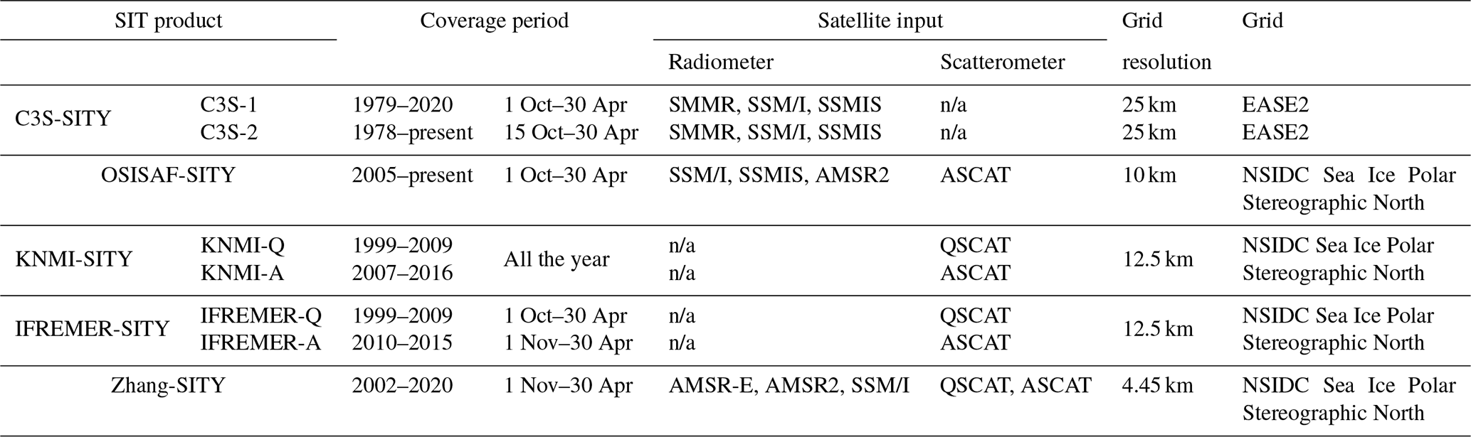
Table 1Basic information of the SITY products.
n/a: not applicable
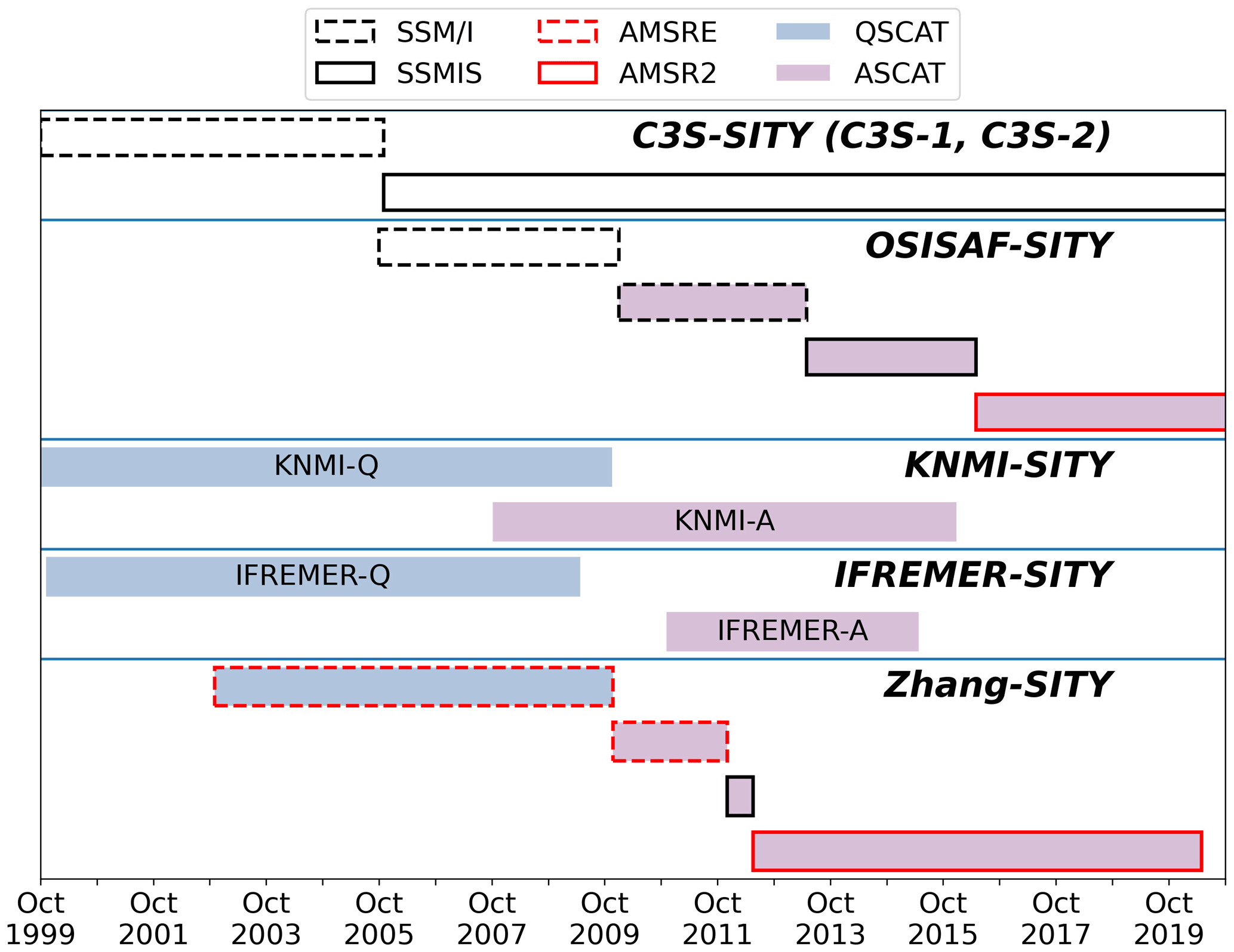
Figure 1The timelines and satellite data input of eight SITY products in this study based on five SITY retrieval schemes.
This study inter-compares eight daily SITY products from five SITY retrieval approaches, including those obtained from the C3S (referred to as C3S-SITY) (Aaboe et al., 2020), Ocean and Sea Ice Satellite Application Facility (referred to as OSISAF-SITY) (Breivik et al., 2012), Royal Netherlands Meteorological Institute (KNMI) (referred to as KNMI-SITY) (Belmonte Rivas et al., 2018), the Satellite Data Processing and Distribution Centre of the French Research Institute for Exploitation of the Sea (CERSAT/Ifremer) (referred to as IFREMER-SITY) (Girard-Ardhuin, 2016), and Beijing Normal University (referred to as Zhang-SITY) (Zhang et al., 2019). Basic information of the SITY products is shown in Table 1, with the timeline of satellite inputs visualized in Fig. 1. Among them, OSISAF-SITY before 2010 and C3S-SITY solely use radiometer data, while KNMI-SITY and IFREMER-SITY only use scatterometer data. In OSISAF-SITY after 2009 and Zhang-SITY, both radiometer and scatterometer measurements are utilized. Retrieval methods of these SITY products are summarized from the aspects of input parameters, classification methods and correction methods (Table 2), with detailed descriptions in the sub-sections below.
Table 2SITY retrieval methods.
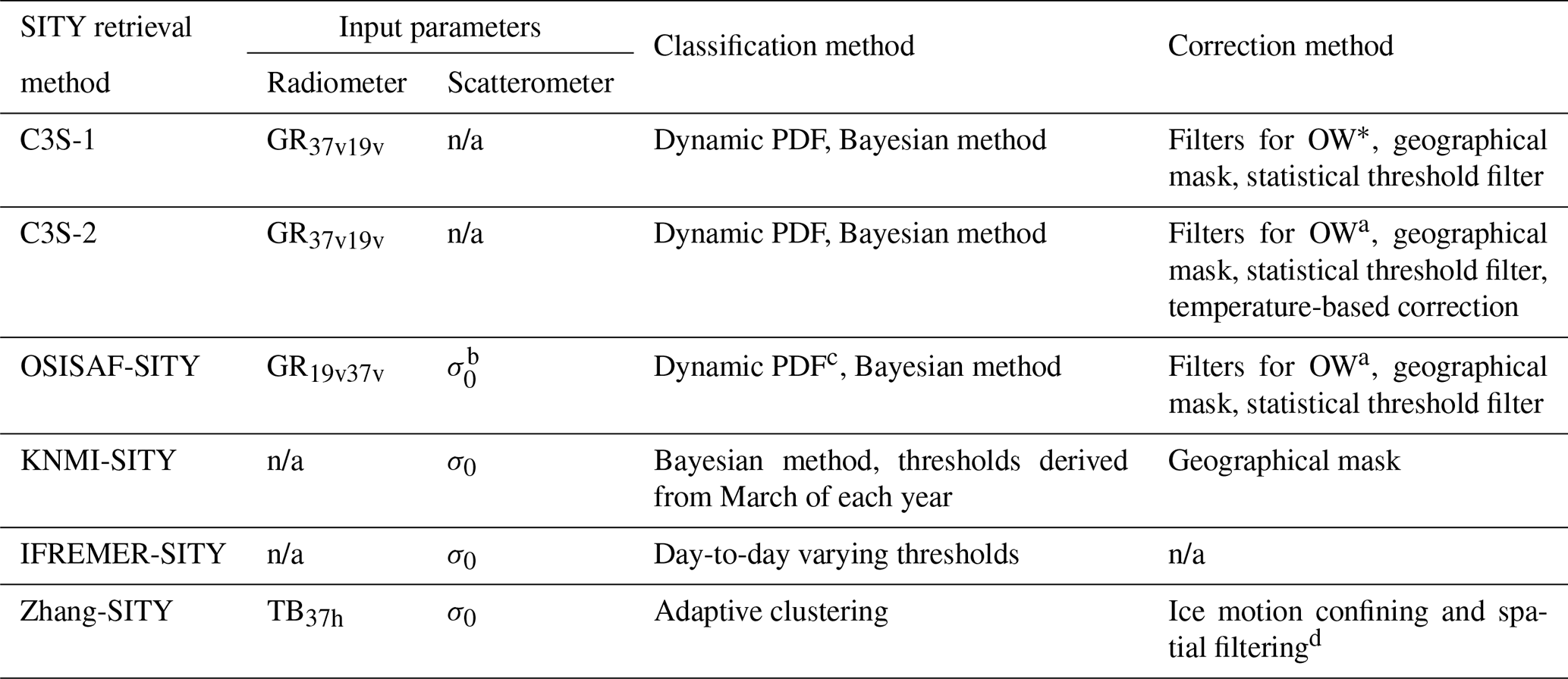
a Filters based on gradient ratio and brightness temperatures are used to filter out spurious sea ice in the open ocean. In this study, discussion of correction methods focuses on those for MYI and FYI. b Scatterometer data from ASCAT were introduced to the OSISAF-SITY retrieval method in 2009. c Dynamical PDF based on daily training data was introduced to the OSISAF-SITY retrieval method in 2015. d Filters considering the impact of ice motion on the temporal changes in SITY (especially MYI) spatial distributions. n/a: not applicable.
2.2.1 C3S-SITY
C3S-SITY is a purely radiometer-based product, provided in the Equal-Area Scalable Earth 2 (EASE2) grid of 25 km spacing. C3S-SITY has been released in two versions. The first version, C3S-1, was released in 2017 and was updated until 2021, covering the period 1979–2020. In 2021, the second version, C3S-2, was released and fully replaced C3S-1 with data available from late 1978 to the present. An upgraded third version is ready to be released at the beginning of 2023 but is not included in this study. SMMR, SSM/I and SSMIS data from the Fundamental Climate Data Record (FCDR) are the primary input data in the C3S-SITY products.
The retrieval of C3S-SITY entails three processing stages: pre-processing, core classification and post-processing.
In the pre-processing, the Tbs are collated and corrected for the land spill-over effects (Maaß and Kaleschke, 2010) and hereafter corrected for atmospheric noise by using a radiative transfer model function with numerical weather prediction data (Wentz, 1997). In the latter process, C3S-1 and C3S-2 differ slightly by using different versions of atmospheric reanalysis from the European Centre for Medium-Range Weather Forecasts (ECMWF), ERA-Interim and ERA-5, respectively. As the last step of the pre-processing, the corrected Tbs swath data are gridded into daily 25 km EASE2 grid Tbs maps using an equal-weighted average (also called a circular top-hat averaging window) of data within a radius from the grid centre (Lavergne et al., 2022).
In the second processing stage, the core of classification is based on a Bayesian approach using the classification parameter GR37v19v. This approach computes the probability of each surface class and selects the most likely class in each pixel. The algorithm is tuned by a daily-updated training dataset of GR37v19v observations collected within the nearest 15 d over pre-defined areas. The daily-updated probability density functions (PDFs) of the collected training data are dynamic in time and capture the seasonal and inter-annual variabilities. The pre-defined areas over which the data are collected are the climatological MYI and FYI regions, which are north of Greenland and Canada with longitudes between 30 and 120∘ W for MYI and the Kara Sea, Baffin Bay, Laptev Sea and the Bay of Bothnia for FYI.
Note that C3S-SITY defines an ambiguous ice type class (referred to as Amb) in addition to the pure MYI and FYI classes. The Amb class represents sea ice with a low classification probability. It may be both pure MYI and FYI or a mixture of FYI and MYI (Aaboe et al., 2021c).
In the last stage, several filters and correction schemes are applied to correct misclassified classes. Open water (OW) filters are applied to remove spurious sea ice in the open ocean; one filter is based on a threshold of GR37v19v to remove erroneously classified ice pixels caused by atmospheric influence, and another filter utilizes 2 m air temperature to exclude the warm water pixels. In addition, the misclassified MYI is re-assigned to FYI partly based on a geographical mask and partly on a statistical threshold filter caused by the overfitted Gaussian distribution of MYI at GR37v19v, which gives rise to an erroneous classification in some extreme cases. Finally, an additional correction scheme based on air temperature is implemented in the C3S-2 algorithm and re-assigns misclassified FYI back to MYI, which is induced by warm air intrusions (Ye et al., 2016a).
2.2.2 OSISAF-SITY
The retrieval behind the OSISAF-SITY product is very similar to C3S-SITY. It differs in being a near-real-time product and being provided in the National Snow and Ice Data Center (NSIDC) Sea Ice Polar Stereographic North projection with 10 km grid spacing. OSISAF-SITY has been available since 2005, however, with regular updates in both the input data and methodology. Therefore, the existing archive of data is not consistent in time, and the quality of the product is expected to be higher nearer to the present time (Aaboe et al., 2021b; Aaboe et al., 2021c). In the period of 2005–2009, OSISAF-SITY is a purely radiometer-based product only using SSM/I as input data. Since 2009, it has been a multi-sensor product when the scatterometer data from ASCAT were introduced to supplement the radiometer data. In 2016, the main radiometer was switched to AMSR2 (Fig. 1).
Unlike C3S-SITY, the core Bayesian computation in OSISAF-SITY is performed on the swath data instead of on gridded data. The computation of PDFs changes in 2015. Before 2015, static PDFs are used in the classifier, which are derived from a fixed training dataset based on observations of the pre-defined areas (same areas as in C3S-SITY) during specific years. Since 2015, dynamic PDFs, based on a daily-updated training dataset like in C3S-SITY, were introduced and have been used ever since. Note that the classification uses the parameter GR37v19v2 solely during 2005–2009 and additionally introduces backscatter from ASCAT (σ0) since 2009. Ice types and their probabilities are derived using classifiers based on the respective observational parameters (GR19v37v and σ0), where swath data of different sensors are used. The probabilities are then gridded based on the distance between each footprint and the polar stereographic grid. The final ice type of each grid is determined by the class with the highest probability. Similar to C3S-SITY, a category of Amb is additionally defined for MYI and FYI in OSISAF-SITY, where the highest ice type probability is less than 75 % (Aaboe et al., 2021b).
In the post-processing stage, OSISAF-SITY uses the same OW filters and masks as those in C3S-SITY, except the final air-temperature correction scheme introduced for C3S-2 to correct for misclassified FYI (Aaboe et al., 2021b).
2.2.3 KNMI-SITY
KNMI-SITY is a series of purely scatterometer-based products with grid spacing of 12.5 km in the NSIDC Sea Ice Polar Stereographic North projection. The scatterometer data used include ERS, QSCAT, OSCAT and ASCAT, which results in four respective SITY products, referred to as KNMI-E, KNMI-Q, KNMI-O and KNMI-A, respectively, available during the periods of 1992–2001, 1999–2009, 2010–2013 and 2007–2016. In this study, KNMI-Q and KNMI-A are included in the comparison considering the comparable input data to other products.
In the pre-processing stage, the ASCAT measurements are normalized to a standard incidence angle of 52.8∘, which is close to that of the VV polarization channel of QSCAT. The normalization is performed according to the dependency of C-band sea ice backscatter on incidence angle (Ezraty and Cavanié, 1999).
In the stage of classification, a refined Bayesian algorithm for ice–water discrimination is first applied to the swath data, based on the probabilistic distances between the observations and the geophysical model functions of ocean wind and sea ice. The swath-based probabilities are then re-gridded to the polar stereographic grid using the averages. The sea ice pixels are eventually classified into FYI, second-year ice (SYI) and older MYI using VV-polarized backscatter with two thresholds, which are determined from the data of March of each year in the Arctic (Belmonte Rivas et al., 2018).
In the last stage, a geographic mask is used to set the erroneously classified MYI pixels back to FYI in the Greenland, Kara, Barents and Chukchi seas.
2.2.4 IFREMER-SITY
IFREMER-SITY is another series of purely scatterometer-based products with grid spacing of 12.5 km in the NSIDC Polar Stereographic North projection. There are two SITY products in IFREMER-SITY, which use QSCAT and ASCAT data for the respective years of 1999–2009 and 2010–2015, referred to as IFREMER-Q and IFREMER-A, respectively.
In the first stage, the backscatter coefficients at different incidence angles (e.g. ASCAT backscatter) are normalized to the value at a constant incidence angle of 40∘ to account for the influence of varying incidence angles. In the core classification, a set of day-to-day varying thresholds are then used for the discrimination between MYI and FYI. These thresholds are derived from the backscatter data of several winters and are found to be inter-annually consistent (Girard-Ardhuin, 2016). Unlike other SITY products, no post-processing has been applied yet in IFREMER-SITY.
2.2.5 Zhang-SITY
Zhang-SITY is a combined SITY product with grid spacing of 4.45 km in the NSIDC Polar Stereographic North projection from 2002 to 2020. Regarding the radiometer data, the AMSR-E and AMSR2 data are prioritized whenever available and are supplemented with SSMIS whenever not. The AMSR-E data are obtained from the NASA Scatterometer Climate Pathfinder (SCP) with a grid spacing of 8.9 km, whereas the AMSR2 and SSMIS data are from GCOM-W1 and NSIDC with a grid spacing of 10 and 25 km, respectively. Scatterometer data from QSCAT and ASCAT are used successively in Zhang-SITY with the QSCAT data until 23 November 2009. All the scatterometer data are obtained from SCP with an enhanced spatial resolution of 4.45 km, as a result of the scatterometer image reconstruction technique (Early and Long, 2001; Long et al., 1993).
In the pre-processing, the ASCAT data are normalized to the value at the incidence angle of 40∘ like that in IFREMER-SITY. All the radiometer and scatterometer data are then re-gridded to the same spacing of 4.45 km using the nearest-neighbour method.
Before ice type classification, open water and low sea ice concentration area are flagged out based on a threshold method using Tbs at the 6.9 GHz V channel. For the ice pixels, an adaptive classification method based on K-means clustering is applied to the observation vectors consisting of Tbs at the 36 GHz H-polarized channel and VV polarization backscatter σ0. It is an unsupervised classification approach and thus does not require the selection of a training dataset. In addition, the results from different sensors are generally consistent, and thus no further processing is conducted for the satellite data (Zhang et al., 2019).
In the last stage, a correction scheme based on sea ice motion and a median filter considering the spatial consistency are used in the post-processing. The former is introduced to eliminate anomalous MYI overestimation, shown as the sudden presence of MYI pixels far away from the estimated MYI pack, based on the MYI temporal record and ice motion. The latter is used to remove large unusual spatial variations in ice types (Zhang et al., 2019).
2.3 Sea ice age product
In this study, the sea ice age (SIA) product from NSIDC is used for inter-comparison, referred to as NSIDC-SIA (Tschudi et al., 2020). NSIDC-SIA is a weekly product available all year round at 12.5 km spacing in the EASE grid from 1984 to 2021. It is derived by tracking trajectories of virtual Lagrangian ice parcels of each grid cell. Ice age (i.e. 1 year, 2 years, … and 5+ years) is assigned according to the number of winters the ice parcels have survived. The age of the oldest ice within the grid cell of each week is regarded as the weekly ice age. The ice motion data used in the tracking process are based on passive microwave observations, as well as auxiliary data such as drifting buoys (Fowler et al., 2004; Maslanik et al., 2011; Tschudi et al., 2020).
NSIDC-SIA has been shown to provide very useful information about the changing Arctic sea ice cover because of its high consistency in long time series (Liu et al., 2016; Meier et al., 2014; Perovich et al., 2020). Due to the scheme of using ice motion data derived from combined satellite and buoy data, NSIDC-SIA supplies a comparable and independent reference for sea ice parameters that are entirely based on remote sensing data, e.g. sea ice type and thickness (Tschudi et al., 2016; Lee et al., 2017).
The accuracy of NSIDC-SIA largely depends on the ice trajectory tracking technique and quality of the ice motion data. There are mainly two sources of error in NSIDC-SIA: the tracking errors related to the coarse resolution of microwave satellite data and those induced by ice motion data vacancy near the coast. The under-sampling of ice motion along with the scheme of oldest ice age assignment leads to an overall discontinuous sea ice age distribution and overestimation of old ice (Korosov et al., 2018). Besides, ice motion velocities from buoys are generally higher than those from satellite data (Sumata et al., 2014). An improper interpolation approach could lead to artificial divergence in ice motion when the buoy estimation differs significantly from the satellite-based data. It could result in approximately 20 % less MYI in the buoy-affected region according to a numerical experiment (Szanyi et al., 2016). Such an impact is mainly found in the years 1983–2005 and has been largely mitigated by tuning the interpolation approach in the current version (Tschudi et al., 2020). Although an adequate evaluation is still needed for the current NSIDC-SIA product, the good consistency and recent upgrades of the interpolation approach make it a useful dataset for SITY comparison.
2.4 Other data
Three Radarsat-1 (referred to as RS-1) and two Sentinel-1 (referred to S-1) SAR images are visually interpreted in terms of ice type classification and used for accuracy assessment in case studies. RS-1 operated from 1995 to 2013, providing C-band (5.3 GHz) SAR images at HH polarization. The incidence angle ranges from 20 to 49∘. S-1 has been operating since 2014, providing C-band (5.4 GHz) SAR images at co- and cross-polarizations with incidence angles between 18.9 to 47.0∘. The three RS-1 images are in ScanSAR wide (SCW) beam mode with a nominal resolution of 100 m, whereas those from S-1 are in extra-wide (EW) swath mode at HH and HV polarizations with a nominal resolution of 40 m. The RS-1 SCW products and the Level-1 Ground Range Detected (GRD) S-1 product are both obtained from the Alaska Satellite Facility. The geolocations and acquisition dates are shown in Fig. 2.
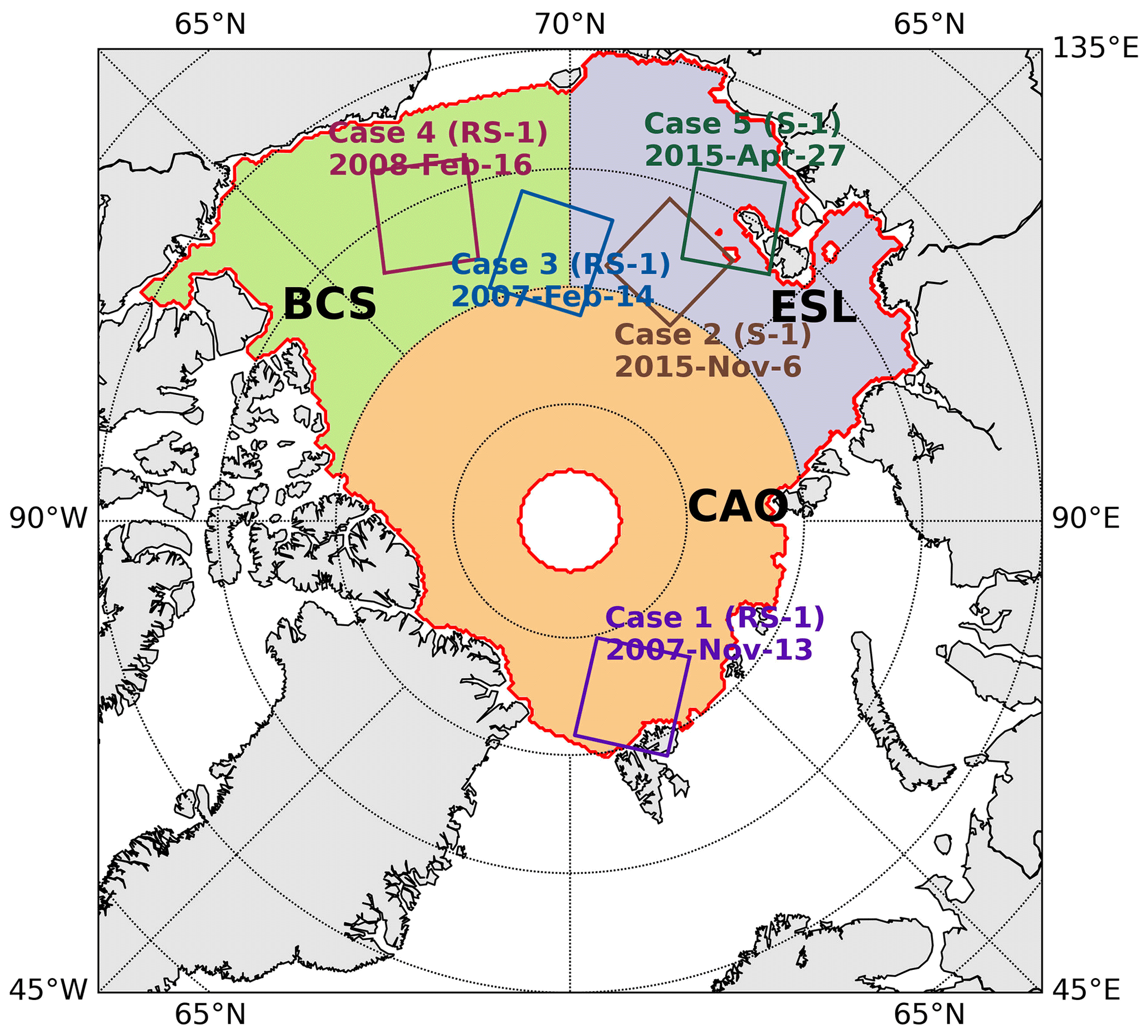
Figure 2Geographic locations of the SAR images for five cases and outline of the Arctic Basin (red contour, provided by Belmonte Rivas et al., 2018). The Arctic Basin is divided into three subregions: the central Arctic Ocean (CAO), the East Siberian and Laptev seas (ESL), and the Beaufort and Chukchi seas (BCS).
Auxiliary data from atmospheric reanalysis are used in addition to the SAR images in the case studies. The reanalysis data include 2 m air temperature and 10 m wind from the ERA5 hourly dataset, produced using 4D-Var data assimilation and model forecasts in CY41R2 of the European Centre for Medium-Range Weather Forecasts (ECMWF) (Hersbach et al., 2018).
3.1 Estimation of MYI extent
For the inter-comparison, the Arctic MYI extent is calculated from the respective SITY and SIA products. The calculations are performed on the area within the Arctic Basin excluding the area north of 87∘ N with its observation data gap due to the inclination of satellites (see Belmonte Rivas et al., 2018, and Fig. 2). Note that the data deficiency area of the SITY products around the North Pole is excluded from the extent calculation and analysis. For the SITY products, the Arctic MYI extent is estimated as the sum of the area of all grid cells specified as MYI within the above-defined area. Both SYI and MYI (ice that is older than 2 years here) classes in KNMI-SITY are included in the MYI extent calculation. The Amb class in C3S-SITY and OSISAF-SITY could be regarded as either MYI or FYI; thus the MYI extent is calculated under both circumstances. This results in two values for the respective SITY products, one for the pixels of MYI class and the other for the pixels of MYI and Amb classes. For NSIDC-SIA, the Arctic extent is calculated as the sum of the area of all grid cells with an ice age of 2 years at least.
As described above, C3S-SITY and NSIDC-SIA are in the EASE grid, while other products are in the polar stereographic grid, with the projection plane tangent to the Earth's surface at 70∘ N. The EASE grid is an equal-areal projection, whereas the polar stereographic grid translates to a 6 % distortion at the North Pole. To account for the areal distortion, all the SITY products in the polar stereographic grids (namely OSISAF-SITY, KNMI-SITY, IFREMER-SITY and Zhang-SITY) are re-projected to the EASE grid before the calculation of MYI extent. In order to compare the MYI extents at the same temporal resolution, the SITY product MYI extents are averaged weekly to match the temporal resolution of NSIDC-SIA.
3.2 Visual interpretation of SAR imagery
SAR imagery has been widely used for SITY classification due to the distinct scattering properties between the major ice types. As described in Sect. 2.1, backscattering from sea ice is predominantly a function of surface scattering for FYI, as well as the combination of surface and volume scattering for MYI. Such a difference is determined by sea ice properties such as salinity, porosity, snow grain size and crystalline structure, as well as the sensor specifications (e.g. frequency, polarization and observation angle) (Gray et al., 1982; Kim et al., 1985). Because of the high spatial resolution, there is additionally texture and shape information from SAR imagery available for ice type discrimination compared to scatterometer data (Holmes et al., 1984). FYI can be formed under calm conditions, resulting in a smooth and level surface, while ridged, rubble or brash ice is formed under turbulent conditions. In contrast, bubble-rich hummocks and much less bubbly refrozen melt ponds are significant features of MYI. Particularly, the MYI floes could develop a clear round shape during the collisions against one another (Onstott, 1992).
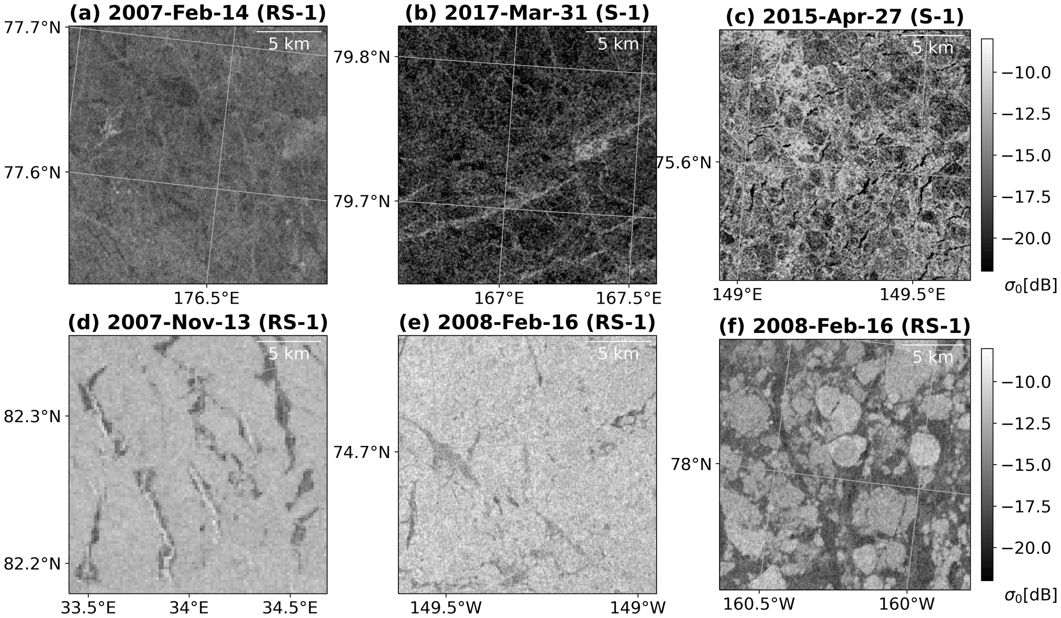
Figure 3Scenes of SAR images (C-band, HH polarization) showing different sea ice features. (a) FYI with smooth textures, (b) FYI with ridged ice in bright linear features, (c) brash ice between ice floes, (d) refrozen leads with bright features, marked with red arrows, (e) MYI with bright backscatter, and (f) MYI floes in a matrix of FYI.
Visual interpretation of SAR images is performed based on the following principles. (1) FYI with level surface exhibits low backscatter signals and smooth textures (Fig. 3a). Ridged FYI presents bright linear structures over the dark background in SAR images (Fig. 3b), while brash ice has high backscatter and is usually found between ice floes (Fig. 3c). (2) Backscatter of newly formed ice is usually low. However, it could be high when frost flowers are formed on the refrozen leads or the ice is rough due to deformation (bright features over the darker strips in Fig. 3d). (3) MYI presents a relatively high backscatter and coarse texture (Fig. 3e). The round floe structures could be used for the identification of MYI (Fig. 3f). (4) Backscatter of OW is dependent on the surface wind. It is low under calm conditions and could be high when the wind speed is high (area D in Fig. 9). The more homogenous texture and lower auto-correlation of OW backscatter could be used to discriminate water from ice in SAR images (Berg and Eriksson, 2012; Aldenhoff et al., 2018). In addition, both the sea ice extent record and the minimum ice extent of the previous summer could be used as additional information for the ice type interpretation from SAR imagery (i.e. classification of OW, FYI and MYI).
Before visual interpretation, all the SAR images are radiometrically calibrated and projected to the respective UTM projection with a pixel size of 50 m for RS-1 data and 40 m for S-1. A refined de-noising method is applied to the S-1 images to reduce the extensive thermal noise at the HV-polarized channel (Sun and Li, 2021). Images at HV polarization are prioritized for the visual interpretation if provided, since the cross-polarized backscattering signals have been shown to increase the separability between MYI and FYI (Gray et al., 1982; Onstott et al., 1979; Dabboor and Geldsetzer, 2014; Song et al., 2021). After the above pre-processing, ice type classification is manually conducted following the aforementioned principles. The classification results are then compared to those from the SITY products for accuracy estimation, when the respective Kappa coefficient and overall accuracy (OA) are calculated. OA represents the probability of overall agreement, denoted as p0:
where n is the number of surface types (i.e. OW, FYI and MYI), and pkk denotes the probability of pixels that are classified as the category k in both the SITY products and SAR interpretation results. Kappa coefficient, denoted as κ, is defined as follows:
where pe represents the random agreement probability, and pik and pkj denote the probabilities of pixels that are classified as the category k in the SITY products and SAR interpretation results, respectively.
This section starts with a temporal and spatial comparison of the SITY products, with NSIDC-SIA as a reference dataset. It then proceeds with a comparison against SAR images. The temporal and spatial comparison provides clues about the overall performance, while the evaluation against SAR images provides more concrete evidence in the five representative cases. For analysis of the spatial patterns, the Arctic is divided into three regions: the central Arctic Ocean (CAO), the East Siberian and Laptev seas (ESL), and the Beaufort and Chukchi seas (BCS).
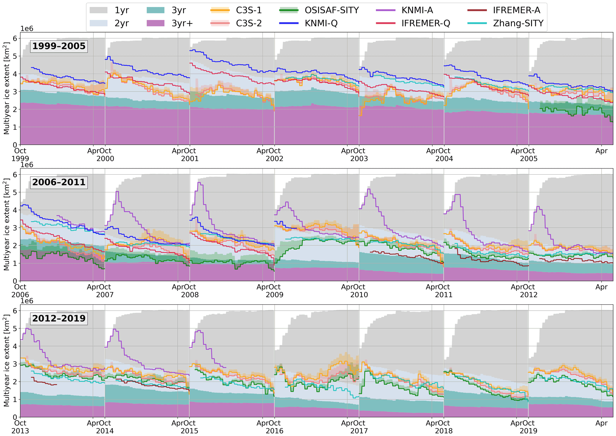
Figure 4Arctic MYI extent variation in SITY products and NSIDC-SIA. The solid line represents weekly MYI extent of the SITY product, the dashed line represents daily MYI extent, and the shaded area in the same colour as the respective solid line represents the ambiguous extent from Amb class (in C3S-1, C3S-2 and OSISAF-SITY), while the stacked block in the background represents ice extent with the corresponding age of NSIDC-SIA.
4.1 Temporal analysis
4.1.1 Weekly MYI extent variation
The Arctic MYI extent from the eight SITY products is compared with the NSIDC-SIA product for the winters from 1999 to 2019 (Fig. 4). The lines represent the weekly MYI extent of each SITY product, with the shaded area indicating the ambiguous extent from Amb class (in C3S-1, C3S-2 and OSISAF-SITY), whereas the stacked block in the background represents the extent for the corresponding age of ice in NSIDC-SIA. Theoretically, since FYI can only turn to MYI when surviving a melting season, the overall Arctic MYI extent cannot increase over the winter – it can only decrease through ice advection out of the Arctic. However, it can temporarily or regionally increase due to ice divergence or advection from neighbouring regions (Kwok et al., 1999).
The SITY products show overall negative trends of the MYI extent within most of the winters as expected. Exceptions occur in some winters for almost all the SITY products. For instance, all the SITY products show increasing MYI extent in March/April 2017 except Zhang-SITY. This could be caused by the enhanced melting during this spring period (Raphael and Handcock, 2022; Ye et al., 2016a), which leads to noise in the radiometric and scattering signatures of MYI similar to that of FYI and therefore unsatisfactory performances of the SITY algorithms. The refined ice motion post-processing technique in Zhang-SITY may help to mitigate such an overestimation problem of MYI (Zhang et al., 2019). Similar increasing patterns are found in October/November of different years for the respective SITY products, e.g. 2001 and 2003 for C3S-SITY, 20093 and 2017 for OSISAF-SITY, and all the years after 2007 for KNMI-A. For C3S-SITY and OSISAF-SITY, such a pattern is caused by the underestimation of MYI in October, while for KNMI-A it is mainly due to the overestimation of MYI in November in the peripheral seas of the Arctic, which will be further discussed in Sect. 5. Note that the other two SITY products (i.e. IFREMER-SITY and Zhang-SITY) do not provide data in October and therefore do not show such a pattern.
Table 3Bias and mean absolute deviation (MAD) between the SITY products and NSIDC-SIA in MYI and FYI extent. Bold font marks the smallest bias and MAD among all the SITY products.
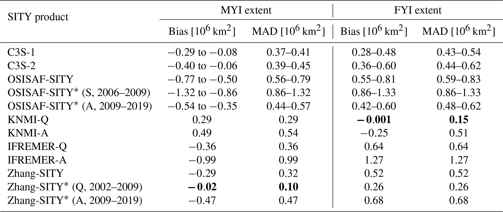
∗: S, Q and A represent the SSMIS, QSCAT and ASCAT periods of the SITY product, respectively.
Table 4Performances of the SITY products compared to SAR images. Bold font highlights the SITY product with the best performance in each case.
∗: the Kappa coefficient and overall accuracy values of C3S-1, C3S-2 and OSISAF-SITY are represented within a lower bound and an upper bound calculated when the Amb class is regarded as FYI and MYI, respectively. ◦: best matches; +/−: overestimates/underestimates MYI; /: overestimates/underestimates MYI in greater degree; n/a: not applicable.
Among all the SITY products, KNMI-SITY, especially KNMI-A, has overall the highest Arctic MYI extent, with a bias of 0.49×10⁶ km2 compared to that from NSIDC-SIA (Table 3). In contrast, OSISAF-SITY in the SSM/I-only period (S, 2006–2009 in Table 4) and IFREMER-A (2012–2015) show the lowest values, with biases of to and km2, respectively. All other SITY products exhibit negative bias in the MYI extent compared to NSIDC-SIA. Among them, Zhang-SITY during the QSCAT period (2002–2009) agrees best with NSIDC-SIA in estimating MYI extent, the average bias and mean absolute deviation (MAD) being and 0.10×10⁶ km2, respectively. Similar to the comparison of MYI extent, we calculate the Arctic FYI extent for the respective SITY and SIA products. All the SITY products exhibit an overestimation of FYI extent (positive bias) compared to NSIDC-SIA except KNMI-SITY (Table 3). KNMI-Q has the best agreement with NSIDC-SIA on FYI extent estimation, with the average bias and MAD of and 0.15×10⁶km2, respectively. Overall, the scatterometer-combined SITY products agree better with NSIDC-SIA than the solely radiometer-based products, e.g. OSISAF-SITY during the ASCAT (2009–2019) and SSMIS periods (2006–2009). The QSCAT-based SITY products are more consistent with NSIDC-SIA than the ASCAT-based products, e.g. KNMI-Q and KNMI-A.
For the SITY products with the Amb class, the average extents of this class are 0.21×10⁶, 0.26×10⁶ and 0.26×10⁶ km2, respectively, for C3S-1, C3S-2 and OSISAF-SITY. As described in Sect. 2.2, these Amb pixels have atypical microwave signatures of MYI–FYI and thus high uncertainties about ice type discrimination. Compared with the average Arctic MYI extent difference against NSIDC-SIA (0.42×10⁶, 0.45×10⁶ and 0.79×10⁶ km2 for C3S-1, C3S-2 and OSISAF-SITY, respectively), the contribution of these pixels to the comparison is overall considerable. In addition, it could be large in situations that trigger the atypical microwave signatures, which will be further discussed in Sect. 4.1.2.
In terms of temporal stabilities, OSISAF-SITY and C3S-SITY (especially C3S-1) show larger day-to-day variabilities in MYI extent than other SITY and SIA products (daily extents not shown). Considering the scatterometer data used in the SITY products (Fig. 1), we find that KNMI-SITY, IFREMER-SITY and Zhang-SITY exhibit larger day-to-day variabilities during the ASCAT period (2009–2019) than the QSCAT period (2002–2009), especially in early winter months such as October and November. In comparison, OSISAF-SITY shows smaller temporal variabilities when backscatter data are used in addition to radiometer data (2009–2019).
Between any two SITY products, the average difference in weekly MYI extent varies between 0.02×10⁶ and 1.92×10⁶ km2 in winter, with values below 1.11×10⁶ km2 during the periods from December to March. The largest difference in weekly MYI extent reaches 4.5×10⁶ km2, which occurs between OSISAF-SITY and KNMI-A in late October 2008. Considering the size of the study region (about 6.5×10⁶ km2), such a discrepancy is significant. This is caused by the relatively low MYI extent from OSISAF-SITY (in the early radiometer-only period) and the exceptional high value from KNMI-A in late October, the reason for which will be discussed in Sect. 5. On the other hand, different SITY products could have consistent MYI extent with nearly negligible difference, which occurs mostly in mid-winter months. Among all, KNMI-Q is most consistent with Zhang-SITY (1999–2008), with weekly MYI extent differences varying between 0.002×10⁶ and 0.79×10⁶ km2.
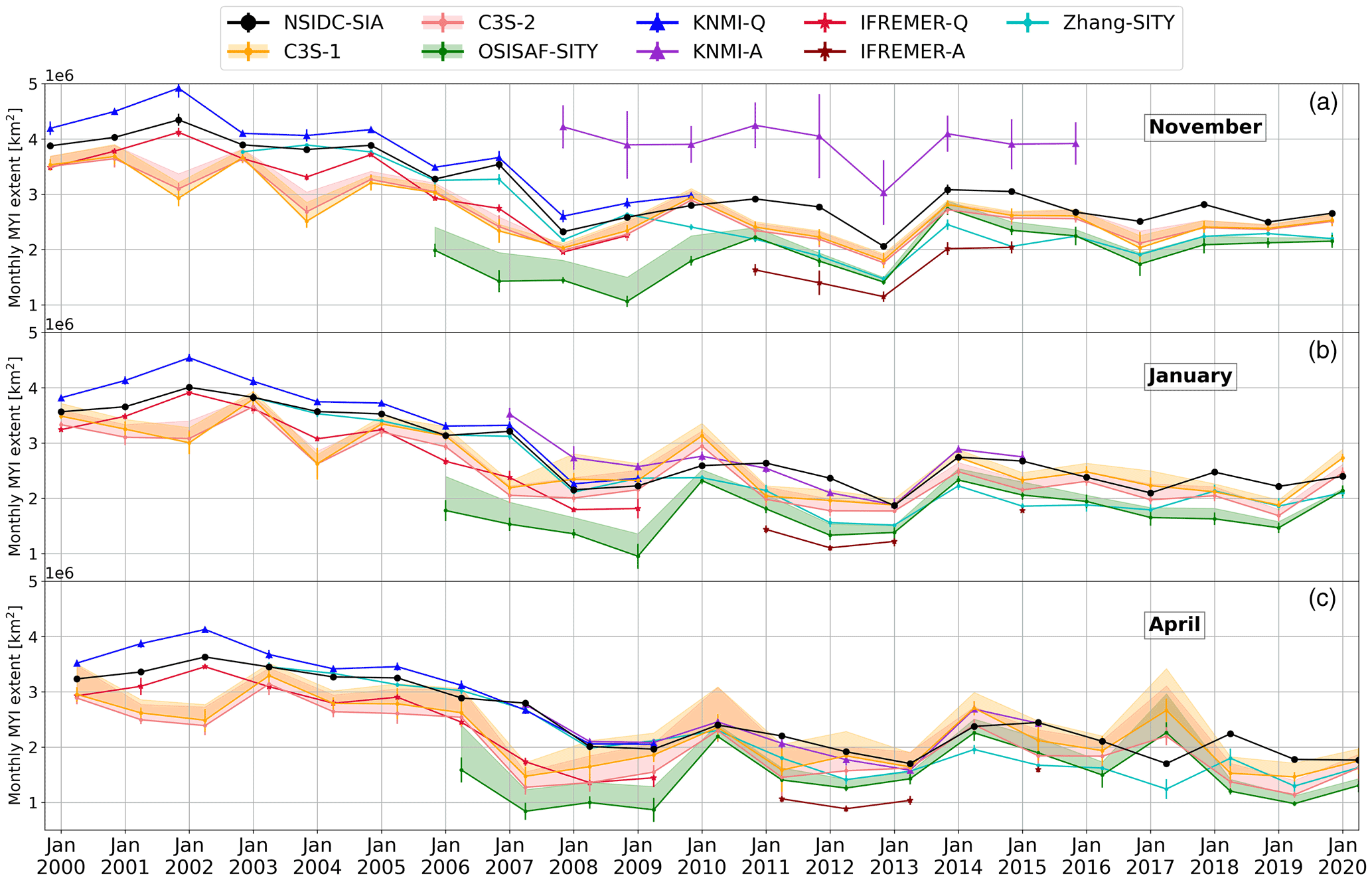
Figure 5Monthly MYI extent of SITY products and NSIDC-SIA in November (a), January (b) and April (c) from November 1999 to April 2020. The shaded area represents the ambiguous extent value for C3S-1, C3S-2 and OSISAF-SITY. The error bar represents the range between maximum and minimum MYI extent in the month.
4.1.2 Monthly MYI extent variation
The monthly average MYI extent of all the SITY and SIA products is presented in Fig. 5, with monthly differences between the respective SITY product and NSIDC-SIA varying from 0.001×10⁶ to 2.3×10⁶ km2. The comparison is demonstrated in 3 months – November, January and April, on behalf of early, middle and late winter, respectively. Overall, the deviation between MYI extent from all the SITY products is the smallest in January. The cold temperatures and relatively stable sea ice physical properties in mid-winter lead to small uncertainties about ice type discrimination. Among the three stages of winter, the deviation between the various SITY products is the largest in early winter, while the extent of the Amb class in C3S-SITY and OSISAF-SITY (shaded area in Fig. 5) is the largest in late winter. Both indicate the difficulties and large discrepancies of SITY products in the transition between summer and winter.
Regarding the inter-annual evolution of MYI extent, C3S-SITY and OSISAF-SITY differ most from other SITY products. OSISAF-SITY exhibits a small negative trend during 2000–2007 and large negative trend from 2007 to 2013, while the former shows larger inter-annual variabilities. This is mainly attributed to the large discrepancies in the winters of 2001–2003, 2006–2008 and 2016–2018. KNMI-Q, IFREMER-Q, IFREMER-A and Zhang-SITY agree well with NSIDC-SIA, with modest discrepancies in all stages of winter. Although the MYI extent from KNMI-A shows the largest discrepancy in early winter, it demonstrates high consistency with NSIDC-SIA in middle and late winter.
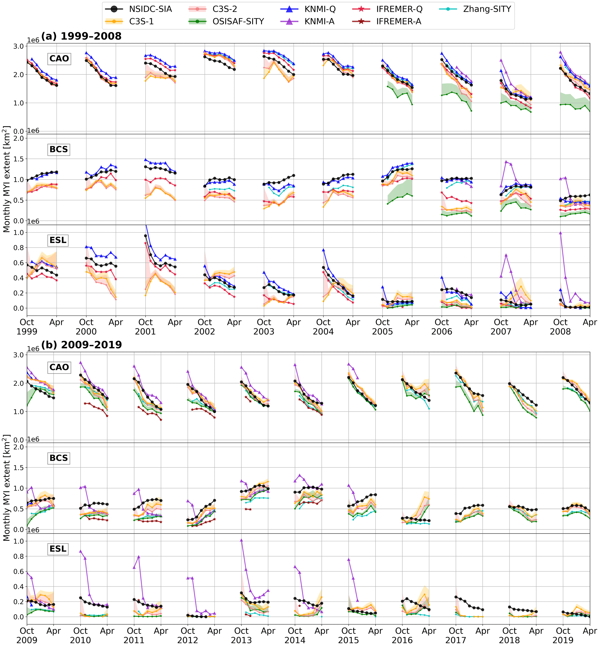
Figure 6Monthly MYI extent of SITY products and NSIDC-SIA in the years (a) 1999–2008 and (b) 2009–2019 in the central Arctic Ocean (CAO), the Beaufort and Chukchi seas (BCS), and the East Siberian and Laptev seas (ESL) (see in Fig. 2). The shaded areas represent the ambiguous extent values for C3S-1, C3S-2 and OSISAF-SITY.
4.2 Spatial analysis
4.2.1 Regional MYI extent evolution
To further explain the classification discrepancies between products, we divided the Arctic into three regions (Fig. 2) and analysed the regional evolution pattern (Fig. 6). Overall, the MYI extent in the CAO and ESL regions shows a consistently negative trend, while the MYI extent in the BCS region remains constant or is increasing. The negative MYI trend in CAO mainly results from the outflow of MYI to more southern areas. On the one hand, MYI is extensively exported through the Fram Strait and, by small fractions, into the Barents Sea and through the Nares Strait (Kuang et al., 2022). In the ESL region, the MYI extent even decreases to zero in some winters (e.g. 2007–2009, 2012–2013), which is in line with the record low Arctic minimum sea ice extent in the previous Septembers. On the other hand, MYI is advected south along the Canadian Arctic Archipelago (CAA) driven by the Beaufort Gyre. In the BCS region, large quantities of MYI enter this region from the north along the CAA and eventually exit BCS westward into ESL or back northward into CAO at the western borders of the BCS region. The nearly constant or increasing MYI extent in the BCS region could be caused by the fact that the MYI extent in BCS reaches a minimum in September and increases toward winter by MYI drifting into it from the north. In the ESL and BCS regions, the NSIDC-SIA MYI extent is usually considerably larger than the MYI extent from the SITY products. In comparison, such a difference is overall smaller in the CAO region. This indicates that the mixture of MYI and FYI (and the medium MYI fraction), which leads to the “overestimated” NSIDC-SIA MYI extent because of the oldest ice age assignment, occurs more frequently in the ESL and BCS regions than the CAO region, which could be explained by the more dynamic ice characteristics in these two regions.
In the winters of 1999–2019, most SITY products show similar intra-seasonal variation in the CAO region while exhibiting different intra-seasonal evolutions in the BCS and ESL regions (especially in early and late winter). For instance, the anomalously large MYI extent from KNMI-SITY in October and November as mentioned before is mainly attributed to the large values in the BCS and ESL regions. The large underestimation of MYI extent in OSISAF-SITY in the CAO and BCS regions before 2010 occurs mainly during the early period of the product before inclusion of the scatterometer data and algorithm upgrades. C3S-SITY shows striking MYI extent fluctuations in 2001–2004 in BCS and ESL, which can partly explain the distinct inter-annual pattern seen in Fig. 5. For C3S-SITY and OSISAF-SITY, the late-winter positive trend in 2016–2017 (Fig. 4) is found in all three regions but is more pronounced in the BCS and ESL regions.
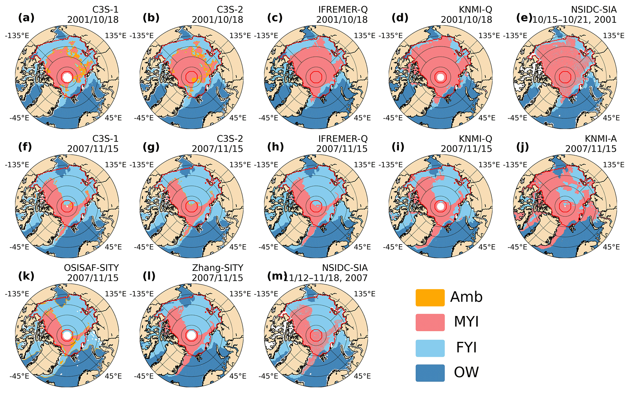
Figure 7Arctic SITY distribution maps from daily SITY products and weekly NSIDC-SIA on 18 October 2001 (a–e) and 15 November 2007 (f–m).
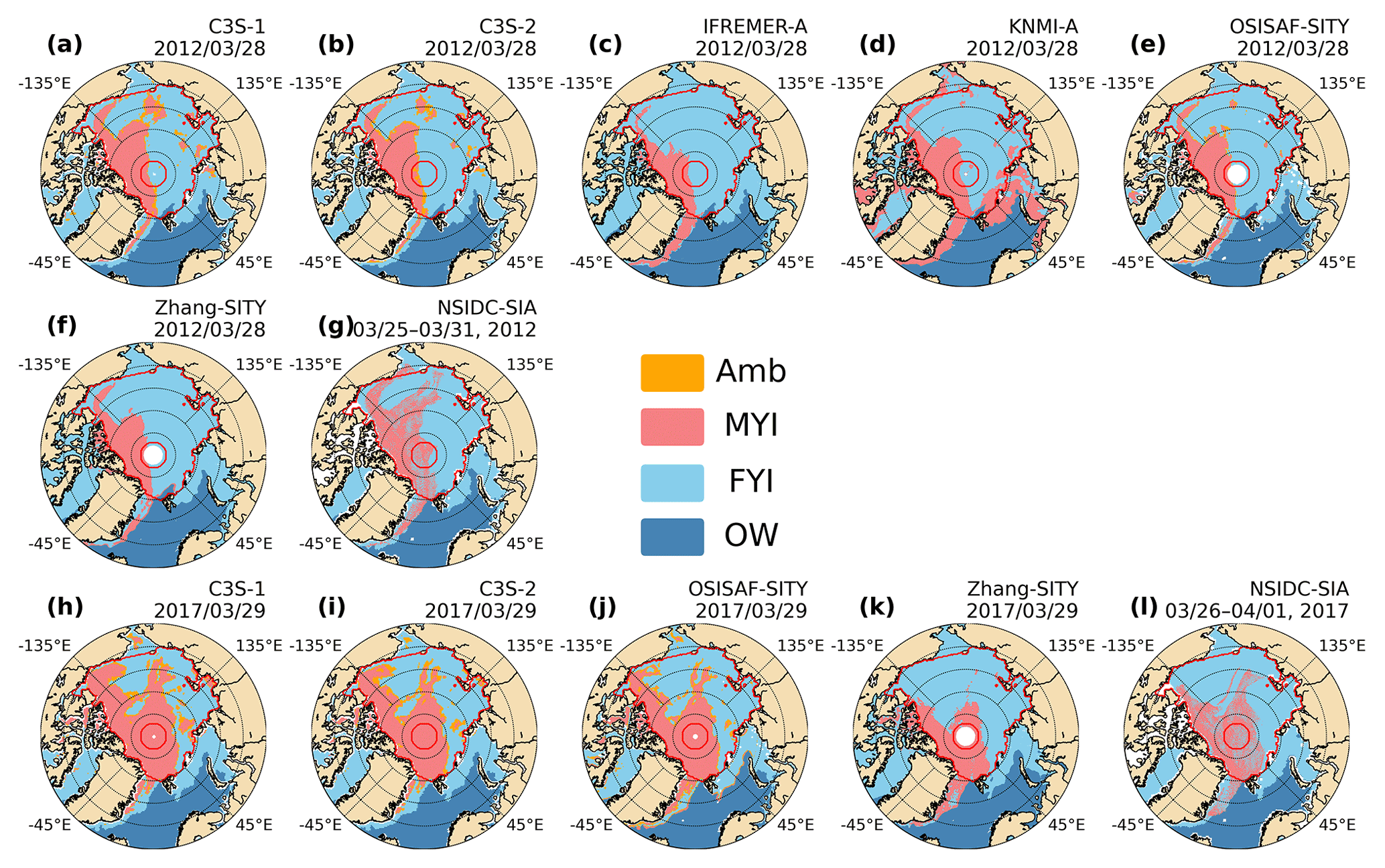
Figure 8Arctic SITY distribution maps from daily SITY products and weekly NSIDC-SIA on 28 March 2012 (a–g) and 29 March 2017 (i–l).
4.2.2 SITY distribution maps
The classification results of SITY products are directly mapped on the perspective of the Arctic for intuitive inter-comparison of the spatial distribution. Figures 7 and 8 show the available SITY and SIA distribution maps, respectively, for the winters of 2001–2002, 2007–2008, 2011–2012 and 2016–2017. Maps of these dates are selected to present typical discrepancies of the SITY products as mentioned in previous sections (see Figs. 4 and 6).
In Fig. 7a–e, the SITY distribution maps of four SITY products and NSIDC-SIA on 18 October 2001 are shown for visual analysis. C3S-SITY shows obviously less MYI than KNMI-Q, IFREMER-Q and NSIDC-SIA, while the latter two SITY products exhibit a quite consistent SITY distribution pattern. The discrepancy of MYI extent between C3S-SITY and NSIDC-SIA is up to 0.29×10⁶ km2 during the winters of 2002–2019. In Fig. 7a and b (along with Fig. A1a–d, f–i in Appendix A), the discontinuous FYI delineation in the inner part of the MYI pack is well demonstrated, which occurs in all winter months and could partly explain the MYI extent fluctuations in C3S-SITY. On the other hand, IFREMER-Q (e.g. Fig. 7c) shows constantly less MYI than KNMI-Q (e.g. Fig. 7d) in the transition zone of MYI and FYI in BCS, which is in good agreement with their difference as shown in Fig. 6.
Figure 7f–m shows the classification maps of seven SITY products and NSIDC-SIA on 15 November 2007. As presented in the previous section, the MYI extent of KNMI-A is much larger than other SITY products in early winter, with exceptionally extensive MYI distributed in the peripheral seas of the Arctic Basin (Fig. 7j). In comparison, KNMI-Q has the second largest MYI coverage among the seven SITY products, with a slightly more finger-like structure of MYI extending through the Chukchi Sea into the ESL region. The other five SITY products show generally consistent SITY distribution patterns as NSIDC-SIA. Minor differences are found in the BCS region. Additionally, C3S-SITY and OSISAF-SITY show notably less MYI in the Fram Strait.
The classification maps in Fig. 8a–g demonstrate a typical scenario with small MYI extent. In the maps of 28 March 2012, the SITY distribution from the SITY products is not as consistent as that from NSIDC-SIA. The difference between NSIDC-SIA and C3S-SITY is the smallest, which could also be reflected in the MYI extent. The weekly MYI extent from NSIDC-SIA is about 1.99×10⁶ km2, whereas it is 1.99×10⁶ and 1.70×10⁶ km2 for C3S-1 and C3S-2 (Amb class not included), respectively. OSISAF-SITY and Zhang-SITY show very similar distribution patterns (Fig. 8e–f), with Arctic MYI extents of about 1.55×10⁶ and 1.30×10⁶ km2, respectively. IFREMER-A shows the smallest MYI extent (1.05×10⁶ km2). KNMI-A differs substantially from other SITY products as in other cases (e.g. Fig. 7f–m). However, the difference is mainly from the Barents and Kara seas in this case, not from the central Arctic as in other cases. Overall, large discrepancies are found among the SITY products, mainly in the BCS region.
Figure 8h–l show the classification of C3S-SITY, OSISAF-SITY, Zhang-SITY and NSIDC-SIA on 29 March 2017. On this day, C3S-SITY and OSISAF-SITY show a consistent SITY distribution as NSIDC-SIA except in BCS, where MYI is overestimated compared to NSIDC-SIA. This overestimation of MYI leads to the abnormal positive trend of MYI extent in BCS and the Arctic during the winter of 2016–2017 in C3S-SITY and OSISAF-SITY (Figs. 4 and 6). Furthermore, the thin tongue-shaped MYI distribution extending across ESL and BCS is not well preserved in Zhang-SITY.
4.3 Evaluation with SAR images
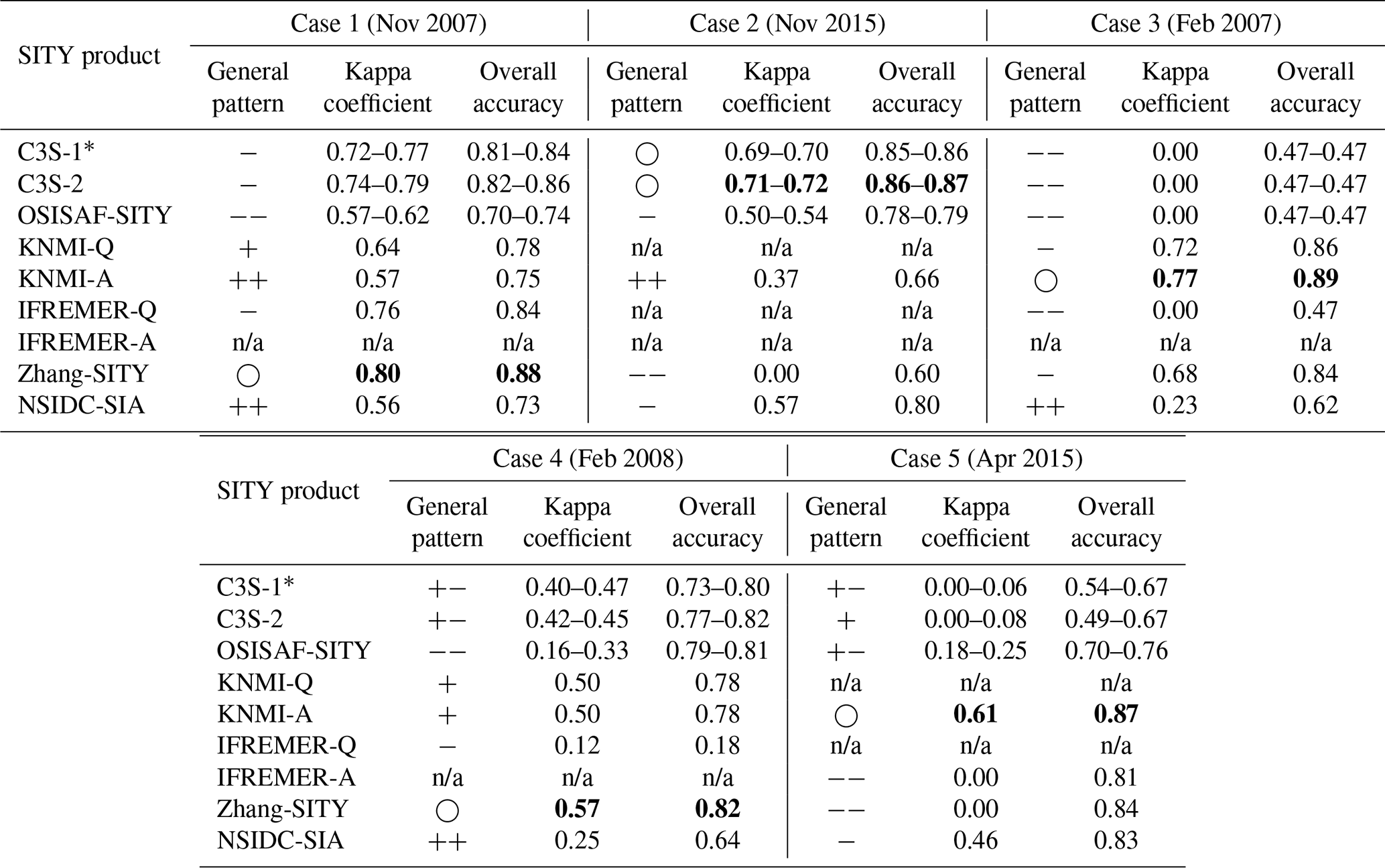
In this section, the SITY products are evaluated using ice type classification results interpreted from RS-1 and S-1 SAR images. Visual interpretation of the SAR images is based on the principles introduced in Sect. 3.2. Five cases are addressed in this study to present SITY distributions under different conditions based on the availability of data and feasibility of visual interpretation. The cases in early and late winter are selected to demonstrate situations with notable discrepancies in the SITY products, whereas the cases in mid-winter are included to explore the performances of the SITY products under relatively steady circumstances. In each case, the SAR image and its interpretation results are presented along with the SITY and SIA products (Figs. 9–13). The Kappa coefficient and OA of the respective SITY product for each case are calculated and presented in Table 4.
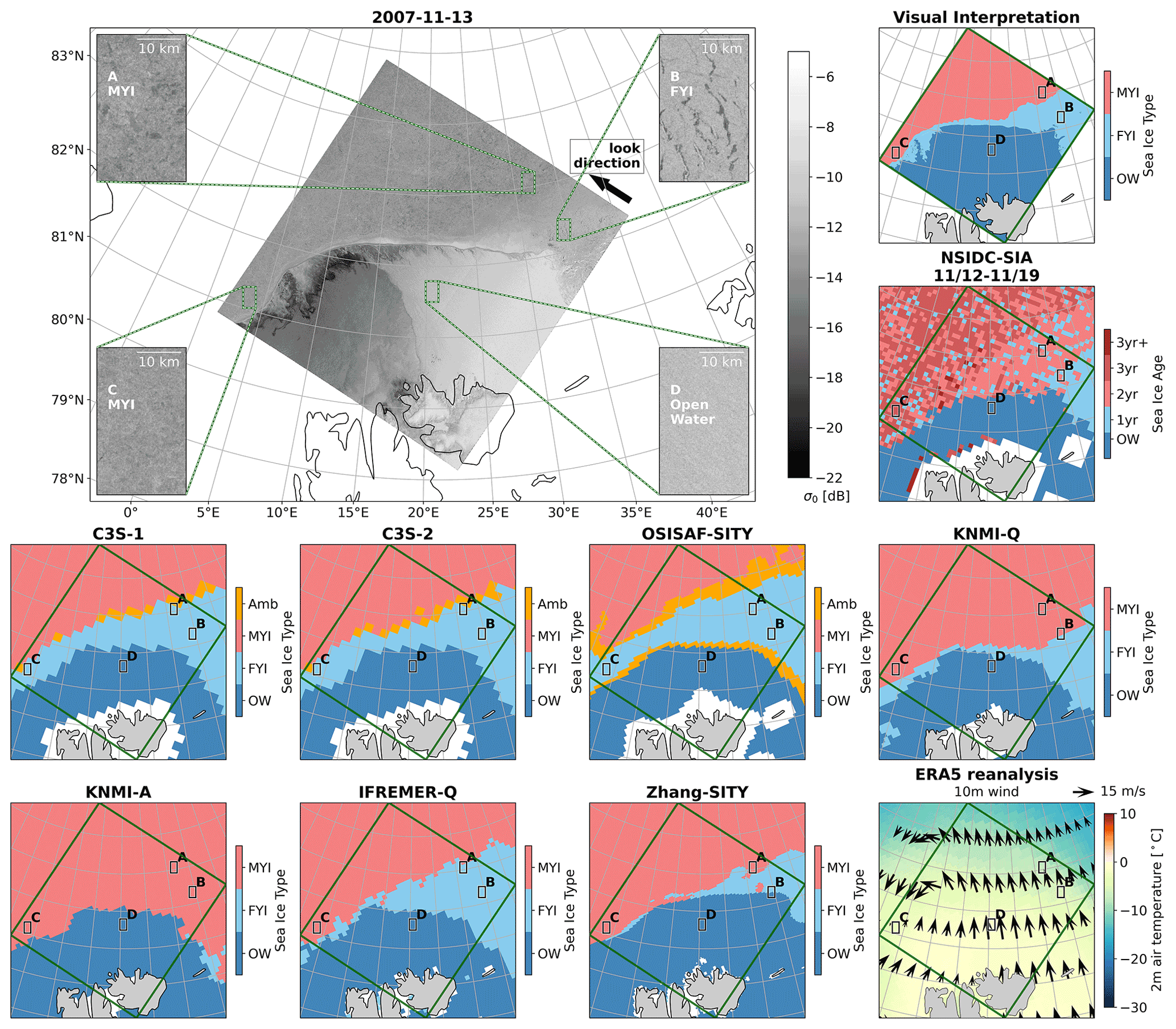
Figure 9RS-1 image, ice type distribution from seven SITY products (C3S-1, C3S-2, OSISAF-SITY, KNMI-Q, KNMI-A, IFREMER-Q and Zhang-SITY), weekly NSIDC-SIA product and visual interpretation result based on the SAR image, along with 2 m air temperature and 10 m wind from ERA5 reanalysis on 13 November 2007.
4.3.1 Cases in early winter
In Case 1, a typical scene of early winter (13 November 2007) in the marginal ice zone is shown in Fig. 9. Compacted ice edges with relatively high backscatter could be observed across the SAR image. In area D, OW manifests high backscatter because of the high wind speed (over 15 m s−1). Sea ice in the west part (area C) with coarse texture appears to be MYI. In the upper part of the image (represented by area A), the coarse texture and darker backscatter signature than area C make it more likely to be MYI which drifts from the central Arctic. At the margin of sea ice and the northeast corner (area B), the quasi-smooth texture, dark backscatter of leads and bright signature of frost flower in between could be interpreted as newly generated FYI. Note that the quality of the SAR interpretation could vary with images. The identified border between FYI and MYI may deviate more from the actual border when the contrast in the backscatter is lower for the different ice types (e.g. Case 1).
The SITY distribution from Zhang-SITY agrees generally well with the SAR image in this case, with the largest OA (0.88) and Kappa coefficient (0.80), although it partly misclassifies FYI as OW or MYI (e.g. area B and the block between areas A and B). Compared with the SAR image, IFREMER-Q shows an underestimation of MYI in area A. C3S-SITY (C3S-1 and C3S-2) and OSISAF-SITY underestimate MYI in areas A and C (note that scatterometer data are not used in OSISAF-SITY in 2007), with slightly less MYI compared to IFREMER-Q. On this day, the wind field was dominated by strong (∼15 m s−1) southerly wind which may explain some of the disagreements shown in daily averaged products in regions close to a border between classes. The KNMI-SITY products overestimate MYI generally. The overestimation is more extensive in KNMI-A (when ASCAT is used), leading to a Kappa coefficient of 0.58 and OA of 0.74 (Table 4). NSIDC-SIA overestimates MYI generally and thus yields a median Kappa coefficient and OA (0.56 and 0.73, respectively). The mobility of ice could partly explain such an overestimation considering the high wind in this region (Fig. 9), which is quite common at the ice edge.
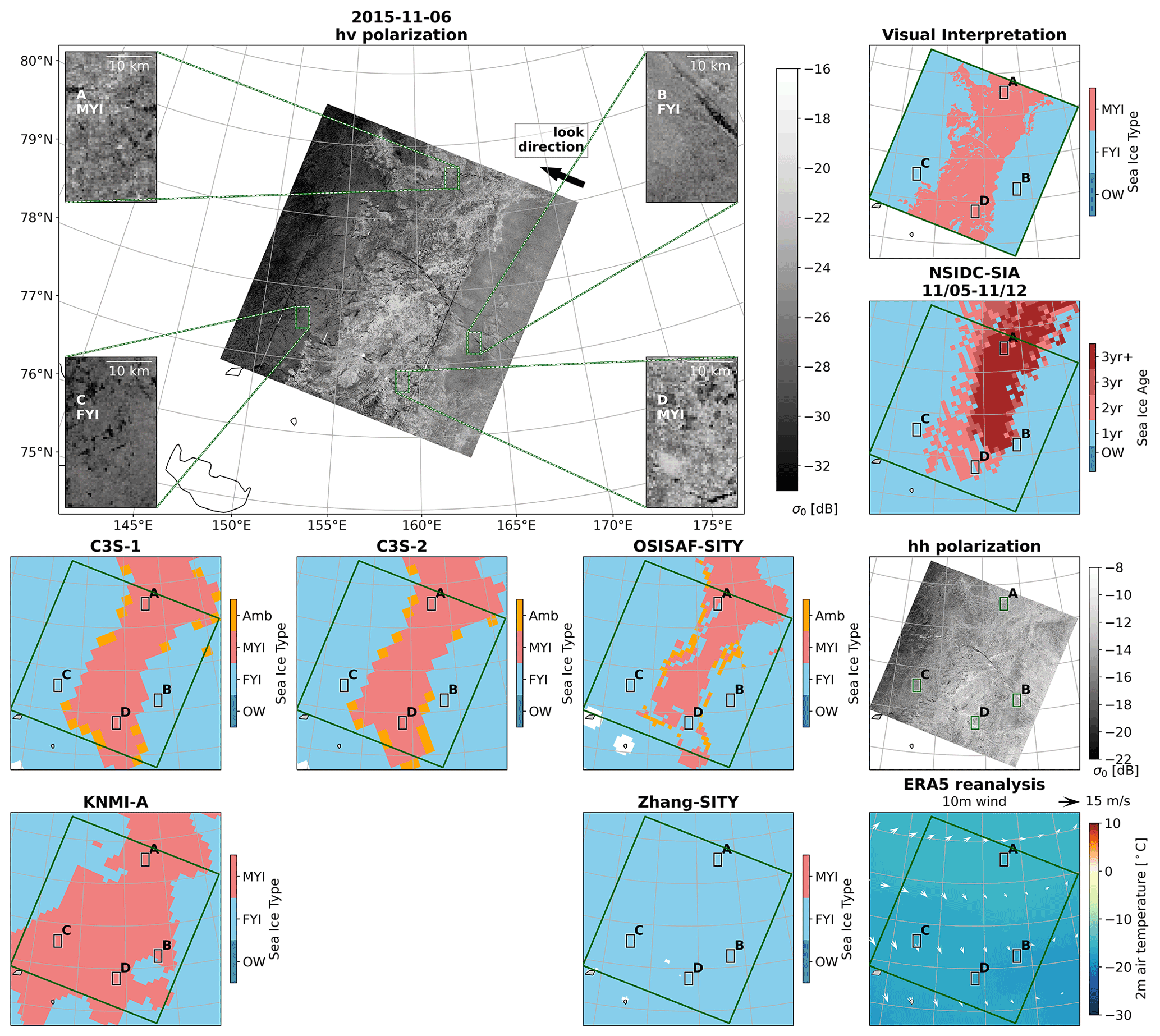
Figure 10HV and HH polarization channels of S-1 image, ice type distribution from five SITY products (C3S-1, C3S-2, OSISAF-SITY, KNMI-A and Zhang-SITY), weekly NSIDC-SIA product, and visual interpretation result based on the SAR image, along with 2 m air temperature and 10 m wind from ERA5 reanalysis on 6 November 2015.
Case 2 is located in the East Siberian Sea on 6 November 2015 (Fig. 10). The air temperature was below −10 ∘C. The wind speed in the western part was higher than in the eastern part. A bright longitudinal feature is clearly shown in the SAR image. It could be identified as MYI with the bright backscatter and coarse texture (area A). In area D, rounded MYI floes can be identified. The east and west part shows low backscatter and smooth texture (enlarged in areas B and C, respectively), which are typical features of FYI. The backscatter signature in area B is brighter than that in area C, influenced by the incidence angle.
The SITY distribution patterns of C3S-SITY (C3S-1 and C3S-2) agree best with the SAR image. As shown in Table 3, the C3S-SITY products have the best performances in this case, with a slightly higher Kappa coefficient in C3S-2. A slight underestimation of MYI can be found in OSISAF-SITY in areas A and D (scatterometer data are used in this case). KNMI-A largely overestimates MYI, especially in the western part of the SAR image. Zhang-SITY totally ignores the MYI pack (narrow MYI tongue across the ESL area, similar to the case in Fig. 8h–l), which lasts for the whole winter (maps not shown). MYI is slightly underestimated in NSIDC-SIA, with a Kappa coefficient of 0.57 and OA of 0.80. Yet such a difference is nearly negligible considering their different temporal resolutions and the mobility features of sea ice.

Figure 11RS-1 image, ice type distribution from seven SITY products (C3S-1, C3S-2, OSISAF-SITY, KNMI-Q, KNMI-A, IFREMER-Q and Zhang-SITY), weekly NSIDC-SIA product and visual interpretation result based on the SAR image, along with 2 m air temperature and 10 m wind from ERA5 reanalysis on 14 February 2007.
4.3.2 Cases in mid-winter
To investigate the constant discrepancies among the SITY products, two cases in mid-winter are selected with focus on the transition zones between MYI and FYI. Case 3 shows the comparison of seven SITY products in Fig. 11, with the RS-1 SAR image located in the region across BCS and ESL, obtained on 14 February 2007. A large area of MYI with high backscatter, ice floe structure and coarse texture could be observed in the centre of the SAR image (area B). Areas A and C present low backscatter and smooth texture, which are typical characteristics of FYI. The backscatter in area D is slightly higher; however, its smooth texture makes it more likely to be FYI.
The general SITY distribution patterns of KNMI-SITY (KNMI-Q and KNMI-A) and Zhang-SITY are basically consistent with the SAR image, with a Kappa coefficient of around 0.7 (Table 4). KNMI-Q and Zhang-SITY slightly underestimate MYI in the southwest corner. IFREMER-Q, C3S-SITY (C3S-1 and C3S-2) and OSISAF-SITY (radiometer-only period) ignore the MYI pack in this area. This regional-scale misclassification of MYI holds through the whole winter (maps not shown). Compared to the SAR image, the SITY distribution in NSIDC-SIA has a distinct pattern, with overestimation of MYI in the northwest part of the image (area A) and underestimation in the northern part (east of area A). As mentioned previously, such discrepancies could be attributed to the mobility features of sea ice and the different temporal resolutions between NSIDC and the SAR image.
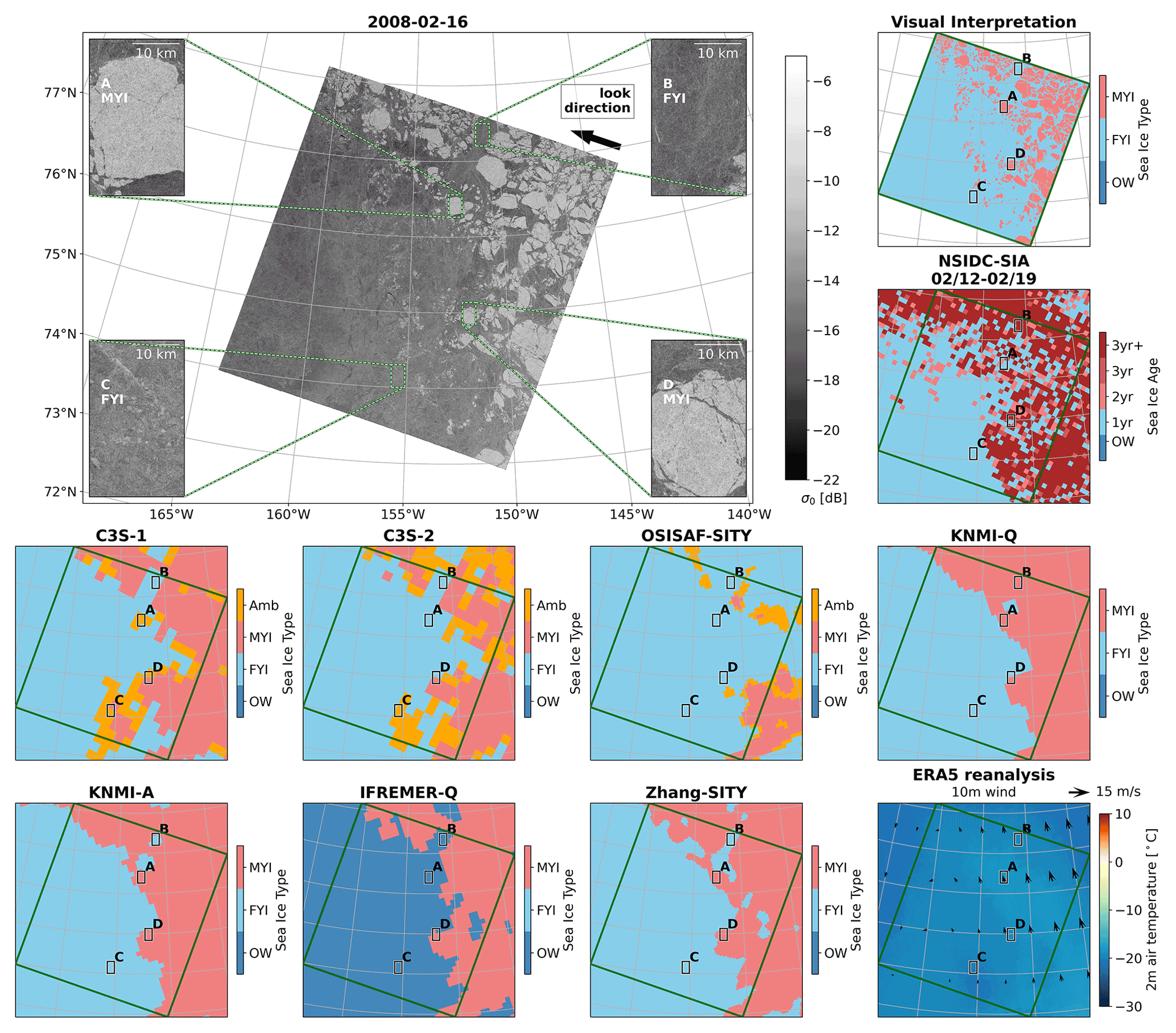
Figure 12RS-1 image, ice type distribution from seven SITY products (C3S-1, C3S-2, OSISAF-SITY, KNMI-Q, KNMI-A, IFREMER-Q and Zhang-SITY), weekly NSIDC-SIA product and visual interpretation result based on the SAR image, along with 2 m air temperature and 10 m wind from ERA5 reanalysis on 16 February 2015.
The fourth case was acquired on 16 February 2008 and is shown in Fig. 12. The bright MYI floe feature is clear in the northeast part of the SAR image and so is the dark FYI feature in the southwest part. Areas A and D exhibit high backscatter of round MYI floe, and areas B and C present typical characteristics of FYI with smooth texture and low backscatter.
The high resolution of the SAR images can clearly show diverse MYI floes within the FYI area (e.g. Fig. 12) and vice versa, which is however not well reflected in SITY products. Taking this into consideration, all the SITY products agree generally well with the SAR image except OSISAF-SITY, which fails to identify the MYI floes in the northeast part. Due to the finer grid resolution, a more detailed SITY distribution is preserved in Zhang-SITY, leading to the largest Kappa coefficient and OA (0.57 and 0.82, respectively). An underestimation of MYI can be found in IFREMER-Q (area A). In addition, IFREMER-Q fails to identify FYI in this case (misclassified as OW), which may be caused by the day-to-day varying thresholds and leads to the lowest Kappa coefficient and OA. KNMI-A manages to identify FYI better than KNMI-Q in area B but overestimates the MYI floes in area D; otherwise the two KNMI-SITY products are very similar. The C3S-SITY products (C3S-1 and C3S-2) are generally consistent with the SAR image but show slight misclassifications in different areas (areas A and C), which may be due to the highly mixed distribution of ice types and coarse resolution. Despite a westward shift, the SITY distribution pattern from NSIDC-SIA is overall similar to the SAR image and indicates a generally older type of MYI (>3 years).
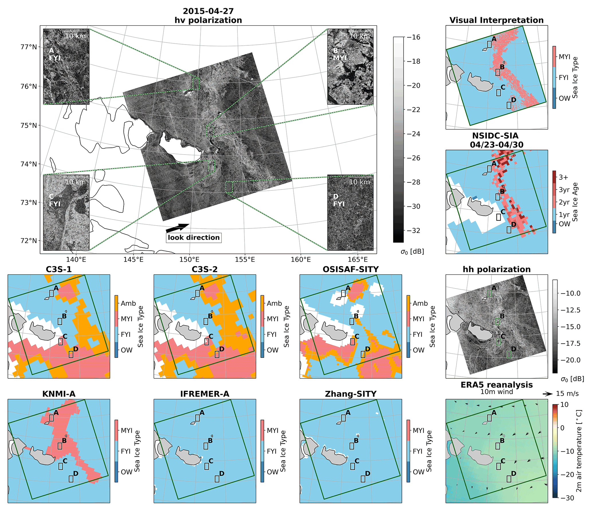
Figure 13HV and HH polarization channels of S-1 image, ice type distribution from six SITY products (C3S-1, C3S-2, OSISAF-SITY, KNMI-A, IFREMER-A and Zhang-SITY), weekly NSIDC-SIA product, and visual interpretation result based on the SAR image, along with 2 m air temperature and 10 m wind from ERA5 reanalysis on 27 April 2015.
4.3.3 Cases in late winter
In Case 5, a S-1 SAR image covering the southern part of ESL near the coast, acquired on 27 April 2015, is shown in Fig. 13. The air temperature was around −10 ∘C. The wind speed and sea ice drift speed were relatively low. The elongated bright feature across the central part of the SAR image appears to be MYI, with a clear floe structure observed in area B. The coarse texture and bright backscatter signature can be found south of the island in the SAR image (area C). As the ice in area C is close/attached to the coast but far away from the minimum sea ice extent of the previous summer, it is more likely to be land-fast ice or deformed FYI rather than MYI. Area A is identified as deformed FYI because of the low-backscatter background and numerous bright linear features of ridges. Area D is interpreted as FYI based on the typical smooth texture and overall dark backscatter signature.
The MYI distribution pattern of KNMI-A resembles the SAR image except for a slight overestimation of MYI in the northern part of the image (area A) and near the island, which may be caused by ice deformation. The Kappa coefficient and OA are the largest for KNMI-A in this case. IFREMER-A and Zhang-SITY both completely ignore the MYI pack. This error starts to occur in November and lasts for the whole winter (maps not shown). C3S-SITY (C3S-1 and C3S-2) and OSISAF-SITY manage to identify FYI in area A and sporadically capture an elongated MYI feature in the northeast part of the image (partly classified as Amb). However, they underestimate MYI in area B and overestimate MYI in the southern part (areas C and D), which leads to a near-zero-level Kappa coefficient. NSIDC-SIA clearly captures the elongated MYI feature in this case, although it has a slight underestimation of MYI in area B.
4.3.4 Performances of sea ice type and age products
Performances of the SITY and SIA products in the above five cases are summarized in Table 4, including the general pattern, Kappa coefficient and OA. In all the five cases, NSIDC-SIA can generally capture the SITY distribution pattern but exhibits a slight over- or underestimation of MYI, which can be explained by the ice age assignment of the oldest ice and different temporal resolution of NSIDC-SIA compared to SAR. These results agree with previous studies (Korosov et al., 2018; Ye et al., 2019) and once again confirm the use of the NSIDC-SIA product as a cross-validation dataset.
In the two cases of early winter (Cases 1 and 2; Figs. 9 and 10), C3S-SITY (C3S-1 and C3S-2) has overall the best performances with a slight underestimation of MYI in Case 1 due to a northward shift in the MYI edge, which can be explained by the persistent southerly wind. In contrast, C3S-SITY totally ignores the identification of MYI in Case 3, leading to a Kappa coefficient of 0. In Cases 4 and 5, C3S-SITY captures the SITY distribution pattern to some extent but does not come out best under different circumstances. Between the two products of C3S-SITY, C3S-2 performs slightly better than C3S-1 with SITY distributions that are more similar to the SAR images in Cases 4 and 5 (Figs. 12 and 13), also reflected in the Kappa coefficient and OA. However, the improvement is insignificant in these five cases.
OSISAF-SITY tends to underestimate MYI in almost all the five cases (Table 4), which is especially obvious for the period before the inclusion of scatterometer data and dynamically updated PDFs (2005–2009, Cases 1, 3 and 4). It shows generally better performance with more recent upgrades of the algorithm, which can also be found in the MYI extent time series (Figs. 4 and 5), where the MYI extent from OSISAF-SITY are more consistent with other SITY and SIA products after 2010.
In contrast to OSISAF-SITY, the KNMI-SITY products (KNMI-Q and KNMI-A) tend to overestimate MYI in the two cases of early winter (Cases 1 and 2) (Table 4). Such an overestimation is especially obvious in KNMI-A and can be found in almost all the winter months. This is well reflected in the extraordinarily large MYI extent of KNMI-A in November (Fig. 5a), which is attributed to the misclassified MYI in the peripheral seas of the Arctic Basin (Fig. 6). In the other three cases, especially Cases 3 and 5, KNMI-SITY has one of the best performances. It manages to preserve the SITY distribution pattern in the cases of middle and late winter. This is in line with the good agreement of MYI extent between KNMI-SITY and NSIDC-SIA in January and April (Fig. 5b and c).
The IFREMER-SITY products (IFREMER-Q and IFREMER-A) tend to underestimate MYI as seen in the time series of MYI extent and case studies. On the other hand, the performance of IFREMER-SITY varies with the cases, which may be caused by the day-to-day varying thresholds and no post-processing to account for the spatio-temporal variations. In Case 1 (Fig. 9), the MYI distribution from IFREMER-Q agrees generally well with the SAR images, with a slight underestimation of MYI. In contrast, it fails to identify the FYI in Case 4 (Fig. 12).
Zhang-SITY performs generally well in the QSCAT period (Cases 1, 3 and 4) with a slight underestimation of FYI and MYI in Cases 1 and 3, respectively. It however fails to identify the thin tongue-shaped MYI pack in the ASCAT period (Cases 2 and 5). Such a pattern is also reflected in the monthly MYI extent time series (Fig. 5), in which the difference between Zhang-SITY and NSIDC-SIA is minimal before 2009 and increases after 2009 (i.e. the ASCAT period).
Performances of the SITY products could be attributed to the following factors: (1) input parameters, (2) classification methods and (3) correction schemes in the post-processing procedure. For further discussion, we analysed the eight SITY products from the above three perspectives (Table 4).
5.1 Input parameters
The efficacy of input parameters depends on their separability of sea ice types and the relevant sea ice physical properties. For instance, the contrast between MYI and FYI is high in the GR37v19v (and GR19v37v) fields. However, this parameter can be impacted by surface features (e.g. snow properties) during the winter (Rostosky et al., 2018; Ye et al., 2019; Comiso, 1983). In the beginning and ending stages of winter, the variability in GR37v19v can be significant when air temperature exhibits warm–cold cycles, which trigger wet–dry cycles or melt–refreeze cycles of snow (Voss et al., 2003; Ye et al., 2016a, b), or when wet or high snow precipitation appears (Voss et al., 2003; Rostosky et al., 2018). This can partly explain the extensive MYI underestimation in the CAO region from C3S-SITY in October (Figs. 6 and 7), as well as the MYI overestimation in BCS and ESL in the second half of winter (Fig. 8). Such a misclassification in C3S-1 is mitigated in C3S-2 due to the upgraded processing, which includes the temperature-based correction in the post-processing and the use of reanalysis data from ERA-5 instead of ERA-Interim in the atmospheric correction for Tb (see Sect. 2.2).
Another example is the backscatter coefficient (σ0), which is commonly used in ice type discrimination due to the different scattering features of MYI and FYI. Backscatter is highly impacted by surface roughness. As a result, deformed FYI, the backscatter of which is relatively high, can be misclassified as MYI when scatterometer data are used. Factors such as snow wetness could also influence the backscatter of sea ice and thus the efficacy. An example is given in Shokr and Agnew (2013), where the increase in snow wetness causes attenuated (decreased) backscatter of MYI and eventually leads to the misclassification of MYI as FYI. In comparison, the backscatter of MYI and FYI differs more at the Ku-band than C-band (Belmonte Rivas et al., 2018; Bi et al., 2020). Products using Ku-band backscatter generally perform better in identifying MYI, e.g. KNMI-Q, IFREMER-Q and Zhang-SITY before 2009. This could be due to the fact that the Ku-band scatterometer is more sensitive to the volume scattering in MYI (Ezraty and Cavanie, 1999). On the other hand, the dominant effect of surface scattering and the higher dependence on incidence angle make C-band backscatter more suitable to distinguish between the ice types with different surface roughness features, e.g. Cases 3 and 4 in Figs. 11 and 12.
It has been shown that the combination of radiometer and scatterometer data helps to identify ice types due to their complementary information (Yu et al., 2009). This statement holds under most conditions in this study (Zhang-SITY in Cases 3 and 4; Figs. 11 and 12). However, when passive and active microwave signatures both behave anomalously, such combination does not help to mitigate the misclassification problems without regulating rules of priority between the two. In the peripheral sea, introducing backscatter does not always help to improve ice type identification in OSISAF-SITY and Zhang-SITY (Case 2; Fig. 10). In the Beaufort and East Siberian seas in late winter, employing Tb and backscatter measurements even leads to the worst SITY classification in Zhang-SITY (Case 5; Fig. 13). This indicates that a simple data combination does not necessarily imply better classification results.
5.2 Classification methods
The representativeness of training datasets and the efficiency of classification methods are crucial for ice type classification. Most SITY products are based on a priori training datasets, which are used to determine the threshold for ice type discrimination. Some algorithms use the thresholds derived from a training dataset that does not vary with time, region or satellite sensors, namely fixed thresholds, while others employ dynamic thresholds to account for the variability in training datasets. The former algorithms work relatively well under conditions similar to the training dataset; however, it gives anomalous SITY distribution results in other conditions. For instance, KNMI-SITY uses the threshold extracted from the mid-winter of each year. Extensive anomalous SITY misclassification is found in the beginning of winter, when the backscatter characteristics of MYI and FYI differ largely from those in mid-winter, especially for C-band backscatter. On the other hand, the dynamic threshold approach considers the spatio-temporal variability in the microwave radiometric and scattering characteristics. However, it may introduce additional temporal instability to the SITY products. The MYI extent from IFREMER-SITY shows high-frequency temporal oscillations in some winters, e.g. in April 2008 (see Fig. 4), which may be caused by the day-to-day varying thresholds used in IFREMER-SITY (see Sect. 2.2.4) and no post-processing to account for the spatio-temporal variations. C3S-SITY and OSISAF-SITY derive PDFs of FYI and MYI from daily training data of fixed target areas. The daily PDFs of the parameter GR37v19v for MYI are highly variable (Aaboe et al., 2021b). The possible explanations could be that the sample area of MYI is susceptible to changes in surface features such as snow properties. Microwave characteristics of the ice samples from a fixed region may not be representative of the whole Arctic Basin, leading to occasionally extensive misclassifications (see Cases 3, 4 and 5; Figs. 11, 12 and 13). This leads to SITY distributions with high-frequency oscillations and large inter-annual variabilities as in the C3S-SITY and OSISAF-SITY products.
An adaptive clustering algorithm is used in Zhang-SITY without a priori training data. The classification depends on the clustering pattern of the two-dimensional scatter of Tb and backscatter. Compared to the QSCAT period (2002–2009), Zhang-SITY shows more anomalous fluctuations and fails to identify such a narrow MYI tongue often observed in Arctic peripheral seas in the ASCAT period (2009–2020). On the one hand, the characteristic microwave signatures of FYI and MYI have more overlaps and thus become more difficult to separate due to the ice loss in the winters over 2007–2009 (Belmonte Rivas et al., 2018). The large loss of old ice (e.g. older than 4 years) in the Arctic Ocean leads to a younger MYI regime in the Arctic (Tschudi et al., 2020) and thus smaller microwave signature differences between MYI and FYI (Belmonte Rivas et al., 2018). On the other hand, because of the lower sensitivity of the C-band scatterometer for MYI identification (as explained in Sect. 5.1), the separation between FYI and MYI becomes more difficult, especially from ASCAT data (Belmonte Rivas et al., 2018; Zhang et al., 2019).
5.3 Correction schemes
Post-processing correction plays an important role in the SITY products. For more accurate SITY distributions, various correction schemes are implemented in the SITY products. These correction schemes can be summarized as follows: (1) corrections based on geographic mask, (2) corrections based on statistical threshold, (3) corrections based on temperature records and the temporal variabilities in SITY distribution, (4) corrections based on the fixed tolerance of ice motion and preceding results, and (5) corrections based on spatial filtering.
The first kind of correction scheme, a mask of the Arctic Basin, has been used in C3S-SITY, OSISAF-SITY and KNMI-SITY to remove the unphysical MYI signature in areas such as the Greenland, Kara, Barents and Chukchi seas. This is restricted to these areas and could not modify classification results within the central Arctic as delineated in this study. The thresholding filter in C3S-SITY and OSISAF-SITY excludes extreme values that are likely to cause misclassification, e.g. values beyond the simulated FYI PDF but within the wide simulated MYI PDF, which usually occurred in ice edge areas (Aaboe et al., 2021b, c). These two kinds of corrections exclude misclassification cases in regions outside the central Arctic and thus have little impact on the overall SITY distributions.
The temperature-based correction in C3S-2 aims to re-assign the ice type MYI to grid cells where MYI was erroneously classified as FYI because it exhibits similar microwave signatures as FYI due to warm air intrusions (Ye et al., 2016a; Shokr and Agnew, 2013). As a result, the discontinuous FYI delineation in the inner part of the MYI pack in C3S-2 is partly mitigated compared to C3S-1 (Fig. A1). In Zhang-SITY, an ice-motion-confining procedure is introduced to eliminate overestimated MYI. The procedure builds upon the ice motion temporal records and confines the evolution of MYI according to the tolerance of ice motion. One drawback of this post-processing is that the wrong re-assignment of MYI to FYI could lead to the continuous underestimation of MYI on consecutive days. Another correction used in Zhang-SITY is the median filter correction, which considers spatial consistency and is employed to remove large unusual SITY spatial variations. These two correction schemes in Zhang-SITY help to mitigate the aforementioned problems. However, inappropriate thresholds in them may lead to over-correction, making Zhang-SITY incapable of identifying the narrow MYI tongue in peripheral seas (Cases 2 and 5; Figs. 10 and 13).
Apart from the above three aspects (input parameters, classification methods and correction schemes), factors such as the coverage period and spatial resolution make the SITY products different from each other. The seasonal length of classification differs from the “all-year” KNMI-SITY products to a limited winter period for other products (see Table 1). In early and late winter larger uncertainties are likely to occur due to processes such as snow metamorphosis and changes in bulk salinity of sea ice (Barber and Thomas, 1998; Voss et al., 2003; Ye et al., 2016a, b). Some SITY products do not provide data in these months (e.g. Zhang-SITY in October); the inter-comparison and evaluation in such conditions thus cannot be done.
In this study, the grid resolution of the SITY products ranges between 4.45 and 25 km. These different resolutions are reflected in the SITY distribution and how well the products capture the smaller-scale features such as ice floes and ice edges. For instance, more detailed information can be found in Zhang-SITY in Case 4 (Fig. 12), whereas C3S-SITY fails to resolve the floe distribution pattern. On the other hand, finer grid spacing does not necessarily mean higher accuracy.
Arctic sea ice cover has decreased dramatically over the past few decades, especially the fraction of MYI. The change in SITY distribution impacts the Arctic and global climate. However, systematic inter-comparison and analyses for SITY products are still lacking. In this paper, eight daily SITY products based on five retrieval approaches were inter-compared through temporal and spatial analysis, with the weekly NSIDC-SIA product as a comparative reference. Performances of them are evaluated qualitatively and quantitatively using five SAR images.
The eight SITY products show overall negative trends of MYI extent as expected within most winters. Exceptions occur mainly in early and late winter months such as October/November and March/April. Compared to NSIDC-SIA, all the SITY products show smaller MYI extent and larger FYI extent except KNMI-SITY (KNMI-Q and KNMI-A). The bias of MYI extent between the SITY products (during the different periods) and NSIDC-SIA varies from km2 (OSISAF-SITY, during the SSM/I-only period, 2006–2009) to 0.49×10⁶ km2 (KNMI-A, 2009–2019). Among all the SITY products, Zhang-SITY in the QSCAT period and KNMI-Q agree best with NSIDC-SIA on the estimation of MYI and FYI extent, respectively.
Between any two SITY products, the difference in weekly MYI extent spans from 0.01×10³ to 4.5×10⁶ km2. The largest discrepancy occurs between OSISAF-SITY and KNMI-A in late October 2008, while the smallest difference is found between KNMI-Q and IFREMER-Q in mid-winter months. It is in line with the spread of the SITY products, which is largest in early winter months such as November and smallest in mid-winter months like January.
Performances of the SITY products can be summarized as follows.
-
C3S-SITY is a pure radiometer-based product. It has the longest temporal record and has been updated to the present day on a daily basis. However, it has large temporal variability and anomalous intra-seasonal trends in MYI extent. It performs generally well in the early winter cases but yields unsatisfactory results in some other winters. The fluctuation and misclassification are likely attributed to the single classification parameter and day-to-day varying training datasets from the pre-defined region, which are vulnerable to weather and ambient conditions and may not be representative of the entire Arctic. C3S-2 performs slightly better than C3S-1 with less misclassification and smaller temporal variability, which could result from the temperature-based correction in post-processing and the upgrades of reanalysis data in the atmospheric correction for Tbs.
-
OSISAF-SITY has an overall underestimation of MYI. Such underestimation is more obvious during the radiometer-only period (2005–2009) while being significantly mitigated due to the upgrades in different periods. The use of additional scatterometer data and finer spatial resolution radiometer data, along with the dynamic PDFs, leads to overall better performance of OSISAF-SITY after 2009; however, there are still large temporal fluctuations in SITY distribution.
-
For the two pure scatterometer-based products, KNMI-SITY tends to overestimate MYI (especially in early winter), while IFREMER-SITY is prone to underestimate MYI. The thresholds used in the classification algorithms play an important role in these two SITY products. KNMI-SITY performs generally well in mid-winter months. The overestimation of MYI occurs mainly in the Arctic peripheral seas in October and November, especially during the C-band scatterometer period (KNMI-A). IFREMER-SITY exhibits high-frequency temporal variations in MYI extent, which could be caused by the day-to-day varying thresholds and improved by including appropriate post-processing.
-
Zhang-SITY exhibits different performances in the two scatterometer periods, with good performance in 2002–2009 (Ku-band scatterometer) and an underestimation of MYI and more anomalous fluctuations after 2009 (C-band scatterometer). During the latter period, it shows difficulties in detecting the thin tongue-shaped distribution of MYI in the Arctic peripheral seas, which could be caused by the excessive correction during post-processing.
Among all the SITY products, KNMI-SITY and Zhang-SITY in the QSCAT period perform the best. In the ASCAT period, KNMI-SITY tends to overestimate MYI (especially in early winter), while Zhang-SITY and IFREMER-SITY tend to underestimate MYI. C3S-SITY performs well in some early winter cases but has large daily variability like OSISAF-SITY and occasionally presents extensive misclassification.
Based on the above inter-comparisons, we further investigate the factors that may impact the SITY production. The main findings can be summarized as follows.
-
The Ku-band scatterometer generally performs better than the C-band scatterometer on ice type discrimination (Belmonte Rivas et al., 2018), while the latter sometimes identifies FYI more accurately, especially when surface scattering dominates the backscatter signature.
-
The simple combination of scatterometer and radiometer data is not always beneficial without further rules of priority between the two.
-
The representativeness of training data and the efficiency of the classification method are crucial for ice type classification. Spatial and temporal variation in the characteristic training dataset should be well accounted for in the SITY method.
-
Post-processing corrections play important roles in SITY products and should be considered with caution. Excessive post-processing such as ice motion confining could lead to an over-correction problem, which becomes the basis for the subsequent corrections and eventually results in accumulative errors.
The accurate estimation of Arctic SITY distribution is crucial for better understanding regional and global climate change, as well as defining sea ice and snow properties for ice thickness retrievals, sea ice models and so on. This study inter-compares eight SITY products and provides hints for further improvement of SITY retrieval approaches. With the new twin-frequency scatterometer (WindRAD, Ku- and C-band) on board the Fengyun (FY)-3E satellite, the potential of scatterometer measurements for ice type discrimination can be further investigated. On the other hand, the Copernicus Imaging Microwave Radiometer with higher spatial resolution at low-frequency channels in the near future opens the opportunity of using low-frequency microwave radiometer measurements for SITY classification (Kilic et al., 2018). In addition to the upgrades of satellite data and improvement of the retrieval approaches, a well-evaluated dataset is still needed for more quantitative inter-comparison and evaluation. An improved sea ice age product from more accurate and higher-resolution ice motion data and well-evaluated ice type interpretation results from SAR images could be the possibilities.
Table A1Specific information of the different sensors, active periods and channels used in the SITY products.
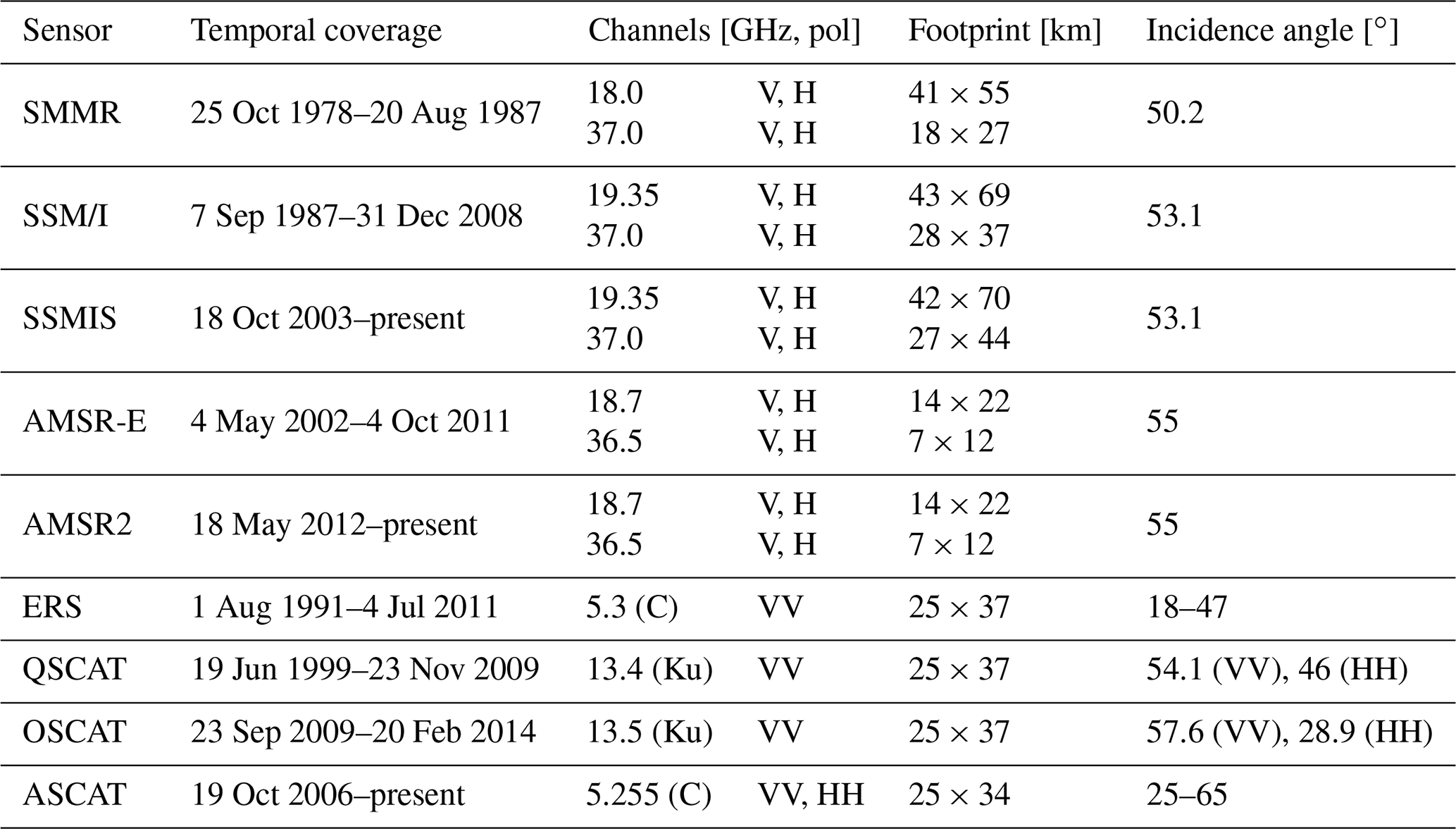
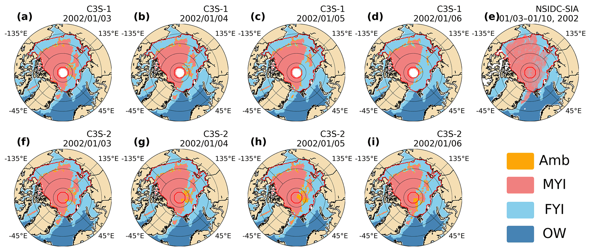
Figure A1Arctic SITY distribution maps from daily SITY product C3S-1 (a–d) and C3S-2 (f–i) and weekly NSIDC-SIA (g) from 3 to 6 January 2002.
C3S-SITY can be obtained from the Copernicus Climate Change Service (C3S) (https://doi.org/10.24381/cds.29c46d83, Aaboe et al., 2020). OSISAF-SITY can be obtained from the Ocean and Sea Ice Satellite Application Facility (OSISAF) (https://osi-saf.eumetsat.int/products/osi-403-d, last access: 1 April 2022). KNMI-SITY is freely available at Royal Netherlands Meteorological Institute (KNMI) (https://dataplatform.knmi.nl/dataset/, last access: 1 April 2022). NSIDC-SIA can be obtained from the National Snow and Ice Data Center (NSIDC) (https://doi.org/10.5067/UTAV7490FEPB; Tschudi et al., 2019). ERA5 reanalysis data are freely available at the European Centre for Medium-Range Weather Forecasts (ECMWF) (https://www.ecmwf.int/en/forecasts/datasets/reanalysis-datasets/era5, last access: 1 April 2022). Radarsat-1 and Sentinel-1 images can be obtained from the Alaska Satellite Facility (ASF) (https://search.asf.alaska.edu/, last access: 1 April 2022). IFREMER-SITY and Zhang-SITY were kindly provided by Fanny Girard-Ardhuin and Zhilun Zhang, respectively, and can be obtained upon request.
YY designed the experiments and led the manuscript writing. YL and YS conducted the data analysis. MS provided access to the SAR images and contributed to the interpretation of the SAR images. YY, YL, SA and FGA contributed to result analysis. FH, XC and ZC contributed to the research design and result analysis. All co-authors participated in the fruitful discussions and manuscript revision.
The contact author has declared that none of the authors has any competing interests.
Publisher's note: Copernicus Publications remains neutral with regard to jurisdictional claims in published maps and institutional affiliations.
The insightful comments from the anonymous reviewers, as well as the editor, are highly acknowledged.
This research has been supported by the National Natural Science Foundation of China (grant no. 42106225), the Innovation Group Project of Southern Marine Science and Engineering Guangdong Laboratory (Zhuhai) (grant no. 311021008), the National Key Research and Development Program of China (grant no. 2019YFC1509104), and the Natural Science Foundation of Guangdong Province (grant no. 2022A1515011545).
This paper was edited by John Yackel and reviewed by three anonymous referees.
Aaboe, S., Sørensen, A., Eastwood, S., and Lavergne, T.: Sea ice edge and type daily gridded data from 1978 to present derived from satellite observations, Climate Data Store [data set], https://doi.org/10.24381/cds.29c46d83, 2020.
Aaboe, S., Down, E., and Eastwood, S.: Global Sea Ice Edge (OSI-402-d) and Type (OSI-403-d) Validation Report, v3.1, in: SAF/OSI/CDOP3/MET-Norway/SCI/RP/224, EUMETSAT OSISAF – Ocean and Sea Ice Satellite Application Facility, 2021a.
Aaboe, S., Down, E., and Eastwood, S.: Algorithm Theoretical Basis Document for the Global Sea-Ice Edge and Type, v3.4, in: SAF/OSI/CDOP3/MET-Norway/TEC/MA/379, EUMETSAT OSISAF: Ocean and Sea Ice Satellite Application Facility, 2021b.
Aaboe, S., Sørensen, A., Lavergne, T., and Eastwood, S.: Sea Ice Edge and Sea Ice Type Climate Data Records Algorithm Theoretical Basis Document, v3.1, EU C3S-Copernicus Climate Change Service, Copernicus Climate Change Service, https://datastore.copernicus-climate.eu/documents/satellite-sea-ice-edge-type/v2.0/D1.SIETy.2-v2.0_ATBD-of-v2.0-SeaIceEdgeType-products_v3.1_APPROVED_Ver1.pdf (last access: 1 April 2022), 2021c.
Aldenhoff, W., Heuzé, C., and Eriksson, L. E. B.: Comparison of ice/water classification in Fram Strait from C- and L-band SAR imagery, Ann. Glaciol., 59, 112–123, https://doi.org/10.1017/aog.2018.7, 2018.
Alexandrov, V., Sandven, S., Wahlin, J., and Johannessen, O. M.: The relation between sea ice thickness and freeboard in the Arctic, The Cryosphere, 4, 373–380, https://doi.org/10.5194/tc-4-373-2010, 2010.
Andersen, S.: Evaluation of SSM/I Sea Ice Algorithms for use in the SAF on Ocean and Sea Ice July 2000, DANISH METEOROLOGICAL INSTITUTE, https://www.dmi.dk/fileadmin/Rapporter/SR/sr00-10.pdf (last access: 1 April 2022), 2000.
Anderson, H. S. and Long, D. G.: Sea ice mapping method for SeaWinds, IEEE T. Geosci. Remote, 43, 647–657, https://doi.org/10.1109/TGRS.2004.842017, 2005.
Barber, D. G. and Thomas, A.: The influence of cloud cover on the radiation budget, physical properties, and microwave scattering coefficient (/spl sigma//spl deg/) of first-year and multiyear sea ice, IEEE T. Geosci. Remote, 36, 38–50, https://doi.org/10.1109/36.655316, 1998.
Belchansky, G. I. and Douglas, D. C.: Classification methods for monitoring Arctic sea ice using OKEAN passive/active two-channel microwave data, Remote Sens. Environ., 73, 307-322, https://doi.org/10.1016/S0034-4257(00)00107-3, 2000.
Belmonte Rivas, M., Verspeek, J., Verhoef, A., and Stoffelen, A.: Bayesian Sea Ice Detection With the Advanced Scatterometer ASCAT, IEEE T. Geosci. Remote, 50, 2649–2657, https://doi.org/10.1109/tgrs.2011.2182356, 2012.
Belmonte Rivas, M., Otosaka, I., Stoffelen, A., and Verhoef, A.: A scatterometer record of sea ice extents and backscatter: 1992–2016, The Cryosphere, 12, 2941–2953, https://doi.org/10.5194/tc-12-2941-2018, 2018.
Belter, H. J., Krumpen, T., von Albedyll, L., Alekseeva, T. A., Birnbaum, G., Frolov, S. V., Hendricks, S., Herber, A., Polyakov, I., Raphael, I., Ricker, R., Serovetnikov, S. S., Webster, M., and Haas, C.: Interannual variability in Transpolar Drift summer sea ice thickness and potential impact of Atlantification, The Cryosphere, 15, 2575–2591, https://doi.org/10.5194/tc-15-2575-2021, 2021.
Berg, A. and Eriksson, L. E. B.: SAR Algorithm for Sea Ice Concentration – Evaluation for the Baltic Sea, IEEE Geosci. Remote Sens. Lett., 9, 938–942, https://doi.org/10.1109/LGRS.2012.2186280, 2012.
Bi, H. B., Liang, Y., Wang, Y. H., Liang, X., Zhang, Z. H., Du, T. Q., Yu, Q. L., Huang, J., Kong, M., and Huang, H. J.: Arctic multiyear sea ice variability observed from satellites: a review, J. Oceanol. Limnol., 38, 962–984, https://doi.org/10.1007/s00343-021-0382-9, 2020.
Boisvert, L. N., Wu, D. L., and Shie, C. L.: Increasing evaporation amounts seen in the Arctic between 2003 and 2013 from AIRS data, J. Geophys. Res.-Atmos., 120, 6865–6881, https://doi.org/10.1002/2015JD023258, 2015.
Breivik, L.-A., Eastwood, S., and Lavergne, T.: Use of C-band scatterometer for sea ice edge identification, IEEE T. Geosci. Remote, 50, 2669–2677, https://doi.org/10.1109/TGRS.2012.2188898, 2012.
Carsey, F.: Summer Arctic sea ice character from satellite microwave data, J. Geophys. Res.-Oceans, 90, 5015–5034, https://doi.org/10.1029/JC090iC03p05015, 1985.
Cavalieri, D. J., Gloersen, P., and Campbell, W. J.: Determination of sea ice parameters with the NIMBUS 7 SMMR, J. Geophys. Res.-Atmos., 89, 5355–5369, https://doi.org/10.1029/JD089iD04p05355, 1984.
Comiso, J. C.: Sea ice effective microwave emissivities from satellite passive microwave and infrared observations, J. Geophys. Res.-Oceans, 88, 7686–7704, https://doi.org/10.1029/JC088iC12p07686, 1983.
Comiso, J. C., Parkinson, C. L., Gersten, R., and Stock, L.: Accelerated decline in the Arctic sea ice cover, Geophys. Res. Lett., 35, L01703, https://doi.org/10.1029/2007GL031972, 2008.
Dabboor, M. and Geldsetzer, T.: Towards sea ice classification using simulated RADARSAT Constellation Mission compact polarimetric SAR imagery, Remote Sens. Environ., 140, 189–195, https://doi.org/10.1016/j.rse.2013.08.035, 2014.
Early, D. S. and Long, D. G.: Image reconstruction and enhanced resolution imaging from irregular samples, IEEE T. Geosci. Remote, 39, 291–302, https://doi.org/10.1109/36.905237, 2001.
Emmerson, C. and Lahn, G.: Arctic opening: Opportunity and risk in the high north, 55, Lloyd's, http://library.arcticportal.org/1671/1/Arctic_O (last access: 1 April 2022), 2012.
Eppler, D. T., Farmer, L. D., Lohanick, A. W., Anderson, M. R., Cavalieri, D. J., Comiso, J., Gloersen, P., Garrity, C., Grenfell, T. C., Hallikainen, M., Maslanik, J. A., MäTzler, C., Melloh, R. A., Rubinstein, I., and Swift, C. T.: Passive Microwave Signatures of Sea Ice, in: Microwave Remote Sensing of Sea Ice, Geophys. Monogr. Ser., 47–71, https://doi.org/10.1029/GM068p0047, 1992.
Ezraty, R. and Cavanie, A.: Construction and evaluation of 12.5-km grid NSCAT backscatter maps over Arctic sea ice, IEEE T. Geosci. Remote, 37, 1685–1697, https://doi.org/10.1109/36.763289, 1999.
Ezraty, R. and Cavanié, A.: Intercomparison of backscatter maps over Arctic sea ice from NSCAT and the ERS scatterometer, J. Geophys. Res.-Oceans, 104, 11471–11483, https://doi.org/10.1029/1998JC900086, 1999.
Fowler, C., Emery, W. J., and Maslanik, J.: Satellite-derived evolution of Arctic sea ice age: October 1978 to March 2003, IEEE Geosci. Remote Sens. Lett., 1, 71–74, https://doi.org/10.1109/LGRS.2004.824741, 2004.
Girard-Ardhuin, F.: Multi-year Arctic sea ice extent estimate from scatterometers onboard satellite since 2000, AGU Fall meeting, San Francisco, CA, USA, 12–16 December, C42B-07, 2016.
Gloersen, P. and Cavalieri, D. J.: Reduction of weather effects in the calculation of sea ice concentration from microwave radiances, J. Geophys. Res.-Oceans, 91, 3913–3919, https://doi.org/10.1029/JC091iC03p03913, 1986.
Gray, A., Hawkins, R., Livingstone, C., Arsenault, L., and Johnstone, W.: Simultaneous scatterometer and radiometer measurements of sea-ice microwave signatures, IEEE J. Ocean. Eng., 7, 20–32, https://doi.org/10.1109/JOE.1982.1145506, 1982.
Hakkinen, S., Proshutinsky, A., and Ashik, I.: Sea ice drift in the Arctic since the 1950s, Geophys. Res. Lett., 35, L19704, https://doi.org/10.1029/2008GL034791, 2008.
Hallikainen, M. and Winebrenner, D. P.: The physical basis for sea ice remote sensing, in: Microwave remote sensing of sea ice, edited by: Carsey, F., American Geophysical Union, 29–46, https://doi.org/10.1029/GM068p0029, 1992.
Hersbach, H., Bell, B., Berrisford, P., Biavati, G., Horányi, A., Muñoz Sabater, J., Nicolas, J., Peubey, C., Radu, R., Rozum, I., Schepers, D., Simmons, A., Soci, C., Dee, D., and Thépaut, J.-N.: ERA5 hourly data on single levels from 1979 to present, Climate Data Store [data set], https://doi.org/10.24381/cds.adbb2d47, 2018.
Holmes, Q. A., Nuesch, D. R., and Shuchman, R. A.: Textural Analysis And Real-Time Classification of Sea-Ice Types Using Digital SAR Data, IEEE T. Geosci. Remote, GE-22, 113–120, https://doi.org/10.1109/TGRS.1984.350602, 1984.
IMarEST: Safety & Sustainability of Shipping and Offshore Activities in the Arctic, Institute of Marine Engineering, Science & Technology, IMarEST Report, London International Shipping Week, 2015.
Jung, T., Kasper, M. A., Semmler, T., and Serrar, S.: Arctic influence on subseasonal midlatitude prediction, Geophys. Res. Lett., 41, 3676–3680, https://doi.org/10.1002/2014GL059961, 2014.
Kern, S., Rösel, A., Pedersen, L. T., Ivanova, N., Saldo, R., and Tonboe, R. T.: The impact of melt ponds on summertime microwave brightness temperatures and sea-ice concentrations, The Cryosphere, 10, 2217–2239, https://doi.org/10.5194/tc-10-2217-2016, 2016.
Kilic, L., Prigent, C., Aires, F., Boutin, J., Heygster, G., Tonboe, R. T., Roquet, H., Jimenez, C., and Donlon, C.: Expected Performances of the Copernicus Imaging Microwave Radiometer (CIMR) for an All-Weather and High Spatial Resolution Estimation of Ocean and Sea Ice Parameters, J. Geophys. Res.-Oceans, 123, 7564–7580, https://doi.org/10.1029/2018JC014408, 2018.
Kim, Y. S., Moore, R. K., Onstott, R. G., and Gogineni, S.: Towards Identification of Optimum Radar Parameters for Sea-Ice Monitoring, J. Glaciol., 31, 214–219, https://doi.org/10.3189/S0022143000006523, 1985.
Korosov, A. A., Rampal, P., Pedersen, L. T., Saldo, R., Ye, Y., Heygster, G., Lavergne, T., Aaboe, S., and Girard-Ardhuin, F.: A new tracking algorithm for sea ice age distribution estimation, The Cryosphere, 12, 2073–2085, https://doi.org/10.5194/tc-12-2073-2018, 2018.
Kuang, H., Luo, Y., Ye, Y., Shokr, M., Chen, Z., Wang, S., Hui, F., Bi, H., and Cheng, X.: Arctic Multiyear Ice Areal Flux and Its Connection with Large-Scale Atmospheric Circulations in the Winters of 2002–2021, Remote Sens., 14, 3742, https://doi.org/10.3390/rs14153742, 2022.
Kwok, R.: Annual cycles of multiyear sea ice coverage of the Arctic Ocean: 1999–2003, J. Geophys. Res., 109, C11004, https://doi.org/10.1029/2003JC002238, 2004.
Kwok, R.: Arctic sea ice thickness, volume, and multiyear ice coverage: losses and coupled variability (1958–2018), Environ. Res. Lett., 13, 105005, https://doi.org/10.1088/1748-9326/aae3ec, 2018.
Kwok, R. and Cunningham, G. F.: Variability of Arctic sea ice thickness and volume from CryoSat-2, Philosophical Transactions of the Royal Society A: Mathematical, Phys. Eng. Sci., 373, 20140157, https://doi.org/10.1098/rsta.2014.0157, 2015.
Kwok, R., Cunningham, G. F., and Yueh, S.: Area balance of the Arctic Ocean perennial ice zone: October 1996 to April 1997, J. Geophys. Res.-Oceans, 104, 25747–25759, https://doi.org/10.1029/1999JC900234, 1999.
Kwok, R., Spreen, G., and Pang, S.: Arctic sea ice circulation and drift speed: Decadal trends and ocean currents, J. Geophys. Res.-Oceans, 118, 2408–2425, https://doi.org/10.1002/jgrc.20191, 2013.
Lavergne, T., Sørensen, A., Tonboe, R. T., Saldo, R., Pedersen, L. T., Strong, C., Cherkaev, E., Golden, K. M., and Eastwood, S.: Algorithm Theoretical Basis Document for the Global Sea-Ice Concentration Climate Data Records, v3.0, In SAF/OSI/CDOP3/DMI_Met/SCI/MA/270, EUMETSAT OSISAF – Ocean and Sea Ice Satellite Application Facility, https://osisaf-hl.met.no/sites/osisaf-hl/files/baseline_document/osisaf_cdop3_ss2_atbd_sea-ice-conc-climate-data-record_v3p0.pdf (last access: 1 April 2022), 2022.
Lee, S.-M., Sohn, B.-J., and Kim, S.-J.: Differentiating between first-year and multiyear sea ice in the Arctic using microwave-retrieved ice emissivities, J. Geophys. Res.-Atmos., 122, 5097–5112, https://doi.org/10.1002/2016JD026275, 2017.
Lindell, D. B. and Long, D.: Multiyear Arctic Ice Classification Using ASCAT and SSMIS, Remote Sens., 8, 294, https://doi.org/10.3390/rs8040294, 2016a.
Lindell, D. B. and Long, D. G.: Multiyear Arctic Sea Ice Classification Using OSCAT and QuikSCAT, IEEE T. Geosci. Remote, 54, 167–175, https://doi.org/10.1109/tgrs.2015.2452215, 2016b.
Liu, J., Curry, J. A., Wang, H., Song, M., and Horton, R. M.: Impact of declining Arctic sea ice on winter snowfall, P. Natl. Acad. Sci. USA, 109, 4074–4079, https://doi.org/10.1073/pnas.1114910109, 2012.
Liu, Q., Babanin, A. V., Zieger, S., Young, I. R., and Guan, C.: Wind and Wave Climate in the Arctic Ocean as Observed by Altimeters, J. Climate, 29, 7957–7975, https://doi.org/10.1175/JCLI-D-16-0219.1, 2016.
Lomax, A. S., Lubin, D., and Whritner, R. H.: The potential for interpreting total and multiyear ice concentrations in SSM/I 85.5 GHz imagery, Remote Sens. Environ., 54, 13–26, https://doi.org/10.1016/0034-4257(95)00082-C, 1995.
Long, D. G., Hardin, P. J., and Whiting, P. T.: Resolution enhancement of spaceborne scatterometer data, IEEE T. Geosci. Remote, 31, 700–715, https://doi.org/10.1109/36.225536, 1993.
Maaß, N. and Kaleschke, L.: Improving passive microwave sea ice concentration algorithms for coastal areas: applications to the Baltic Sea, Tellus A, 62, 393–410, https://doi.org/10.1111/j.1600-0870.2010.00452.x, 2010.
Maslanik, J., Stroeve, J., Fowler, C., and Emery, W.: Distribution and trends in Arctic sea ice age through spring 2011, Geophys. Res. Lett., 38, L13502, https://doi.org/10.1029/2011GL047735, 2011.
Maslanik, J. A., Fowler, C., Stroeve, J., Drobot, S., Zwally, J., Yi, D., and Emery, W.: A younger, thinner Arctic ice cover: Increased potential for rapid, extensive sea-ice loss, Geophys. Res. Lett., 34, L24501, https://doi.org/10.1029/2007GL032043, 2007.
Meier, W. N., Hovelsrud, G. K., Van Oort, B. E. H., Key, J. R., Kovacs, K. M., Michel, C., Haas, C., Granskog, M. A., Gerland, S., Perovich, D. K., Makshtas, A., and Reist, J. D.: Arctic sea ice in transformation: A review of recent observed changes and impacts on biology and human activity, Rev. Geophys., 52, 185–217, https://doi.org/10.1002/2013rg000431, 2014.
Onarheim, I. H., Eldevik, T., Smedsrud, L. H., and Stroeve, J. C.: Seasonal and Regional Manifestation of Arctic Sea Ice Loss, J. Climate, 31, 4917–4932, https://doi.org/10.1175/jcli-d-17-0427.1, 2018.
Onstott, R. G.: SAR and Scatterometer Signatures of Sea Ice, in: Microwave Remote Sensing of Sea Ice, Geophys. Monogr. Ser., 73–104, https://doi.org/10.1029/GM068p0073, 1992.
Onstott, R. G., Moore, R. K., and Weeks, W. F.: Surface-Based Scatterometer Results of Arctic Sea Ice, IEEE T. Geosci. Electron., 17, 78–85, https://doi.org/10.1109/TGE.1979.294616, 1979.
Perovich, D., Meier, W., Tschudi, M., Hendricks, S., Petty, A. A., Divine, D., Farrell, S., Gerland, S., Haas, C., Kaleschke, L., Pavlova, O., Ricker, R., Tian-Kunze, X., Webster, M., and Wood, K.: Sea ice, in: Arctic report card 2020, NOAA, https://doi.org/10.25923/n170-9h57, 2020.
Perovich, D., Meier, W., Tschudi, M., Farrell, S., Hendricks, S., Gerland, S., Kaleschke, L., Ricker, R., Tian-Kunze, X., Webster, M., and Wood, K.: Sea ice, in: Arctic Report Card 2021, NOAA, https://doi.org/10.25923/y2wd-fn85, 2021.
Petty, A. A., Kurtz, N. T., Kwok, R., Markus, T., and Neumann, T. A.: Winter Arctic sea ice thickness from ICESat-2 freeboards, J. Geophys. Res.-Oceans, 125, e2019JC015764, https://doi.org/10.1029/2019JC015764, 2020.
Raphael, M. N. and Handcock, M. S.: A new record minimum for Antarctic sea ice, Nat. Rev. Earth Environ., 3, 215–216, https://doi.org/10.1038/s43017-022-00281-0, 2022.
Rostosky, P., Spreen, G., Farrell, S. L., Frost, T., Heygster, G., and Melsheimer, C.: Snow Depth Retrieval on Arctic Sea Ice From Passive Microwave RadiometersImprovements and Extensions to Multiyear Ice Using Lower Frequencies, J. Geophys. Res.-Oceans, 123, 7120–7138, https://doi.org/10.1029/2018jc014028, 2018.
Rothrock, D. A., Percival, D. B., and Wensnahan, M.: The decline in arctic sea-ice thickness: Separating the spatial, annual, and interannual variability in a quarter century of submarine data, J. Geophys. Res.-Oceans, 113, C05003, https://doi.org/10.1029/2007JC004252, 2008.
Screen, J. A., Simmonds, I., Deser, C., and Tomas, R.: The atmospheric response to three decades of observed Arctic sea ice loss, J. Climate, 26, 1230–1248, https://doi.org/10.1175/JCLI-D-12-00063.1, 2013.
Shokr, M. E.: Field observations and model calculations of dielectric properties of Arctic sea ice in the microwave C-band, IEEE T. Geosci. Remote, 36, 463–478, https://doi.org/10.1109/36.662730, 1998.
Shokr, M. and Agnew, T. A.: Validation and potential applications of Environment Canada Ice Concentration Extractor (ECICE) algorithm to Arctic ice by combining AMSR-E and QuikSCAT observations, Remote Sens. Environ., 128, 315–332, https://doi.org/10.1016/j.rse.2012.10.016, 2013.
Shokr, M. and Sinha, N. K.: Sea ice: physics and remote sensing, John Wiley & Sons, American Geophysical Union, ISBN 978-1-119-02789-8, 2015.
Shokr, M., Lambe, A., and Agnew, T.: A New Algorithm (ECICE) to Estimate Ice Concentration From Remote Sensing Observations: An Application to 85-GHz Passive Microwave Data, IEEE T. Geosci. Remote, 46, 4104–4121, https://doi.org/10.1109/TGRS.2008.2000624, 2008.
Song, W., Li, M., Gao, W., Huang, D., Ma, Z., Liotta, A., and Perra, C.: Automatic Sea-Ice Classification of SAR Images Based on Spatial and Temporal Features Learning, IEEE T. Geosci. Remote, 59, 9887–9901, https://doi.org/10.1109/TGRS.2020.3049031, 2021.
Sumata, H., Lavergne, T., Girard-Ardhuin, F., Kimura, N., Tschudi, M. A., Kauker, F., Karcher, M., and Gerdes, R.: An intercomparison of Arctic ice drift products to deduce uncertainty estimates, J. Geophys. Res.-Oceans, 119, 4887–4921, https://doi.org/10.1002/2013JC009724, 2014.
Sun, Y. and Li, X.-M.: Denoising Sentinel-1 Extra-Wide Mode Cross-Polarization Images Over Sea Ice, IEEE T. Geosci. Remote, 59, 2116–2131, https://doi.org/10.1109/TGRS.2020.3005831, 2021.
Swan, A. M. and Long, D. G.: Multiyear Arctic Sea Ice Classification Using QuikSCAT, IEEE T. Geosci. Remote, 50, 3317–3326, https://doi.org/10.1109/tgrs.2012.2184123, 2012.
Szanyi, S., Lukovich, J. V., Barber, D. G., and Haller, G.: Persistent artifacts in the NSIDC ice motion data set and their implications for analysis, Geophys. Res. Lett., 43, 10800–10807, https://doi.org/10.1002/2016GL069799, 2016.
Tschudi, M. A., Stroeve, J. C., and Stewart, J. S.: Relating the Age of Arctic Sea Ice to its Thickness, as Measured during NASA's ICESat and IceBridge Campaigns, Remote Sens., 8, 457, https://doi.org/10.3390/rs8060457, 2016.
Tschudi, M. A., Meier, W. N., and Stewart, J. S.: An enhancement to sea ice motion and age products at the National Snow and Ice Data Center (NSIDC), The Cryosphere, 14, 1519–1536, https://doi.org/10.5194/tc-14-1519-2020, 2020.
Tschudi, M., Meier, W. N., Stewart, J. S., Fowler, C., and Maslanik, J.: EASE-Grid Sea Ice Age, Version 4, Boulder, Colorado USA. NASA National Snow and Ice Data Center Distributed Active Archive Center [data set], https://doi.org/10.5067/UTAV7490FEPB, 2019.
Vant, M. R., Ramseier, R. O., and Makios, V.: The complex-dielectric constant of sea ice at frequencies in the range 0.1–40 GHz, J. Appl. Phys., 49, 1264–1280, https://doi.org/10.1063/1.325018, 1978.
Voss, S., Heygster, G., and Ezraty, R.: Improving sea ice type discrimination by the simultaneous use of SSM/I and scatterometer data, Polar Res., 22, 35–42, https://doi.org/10.1111/j.1751-8369.2003.tb00093.x, 2003.
Walker, N. P., Partington, K. C., Woert, M. L. V., and Street, T. L. T.: Arctic Sea Ice Type and Concentration Mapping Using Passive and Active Microwave Sensors, IEEE T. Geosci. Remote, 44, 3574–3584, https://doi.org/10.1109/TGRS.2006.881116, 2006.
Weeks, W. F. and Ackley, S. F.: The Growth, Structure, and Properties of Sea Ice, in: The Geophysics of Sea Ice, edited by: Untersteiner, N., Springer US, Boston, MA, 9–164, https://doi.org/10.1007/978-1-4899-5352-0_2, 1986.
Wentz, F. J.: A well-calibrated ocean algorithm for special sensor microwave/imager, J. Geophys. Res.-Oceans, 102, 8703–8718, https://doi.org/10.1029/96JC01751, 1997.
Xu, R., Zhao, C., Zhai, X., and Chen, G.: Arctic Sea Ice Type Classification by Combining CFOSCAT and AMSR-2 Data, Earth Space Sci., 9, e2021EA002052, https://doi.org/10.1029/2021EA002052, 2022.
Ye, Y., Heygster, G., and Shokr, M.: Improving Multiyear Ice Concentration Estimates With Reanalysis Air Temperatures, IEEE T. Geosci. Remote, 54, 2602–2614, https://doi.org/10.1109/TGRS.2015.2503884, 2016a.
Ye, Y., Shokr, M., Heygster, G., and Spreen, G.: Improving multiyear sea ice concentration estimates with sea ice drift, Remote Sens., 8, 397, https://doi.org/10.3390/rs8050397, 2016b.
Ye, Y., Shokr, M., Aaboe, S., Aldenhoff, W., Eriksson, L. E. B., Heygster, G., Melsheimer, C., and Girard-Ardhuin, F.: Inter-comparison and evaluation of sea ice type concentration algorithms, The Cryosphere Discuss. [preprint], https://doi.org/10.5194/tc-2019-200, 2019.
Yu, P., Clausi, D. A., and Howell, S.: Fusing AMSR-E and QuikSCAT Imagery for Improved Sea Ice Recognition, IEEE T. Geosci. Remote, 47, 1980–1989, https://doi.org/10.1109/tgrs.2009.2013632, 2009.
Zhang, Z., Yu, Y., Li, X., Hui, F., Cheng, X., and Chen, Z.: Arctic Sea Ice Classification Using Microwave Scatterometer and Radiometer Data During 2002–2017, IEEE T. Geosci. Remote, 57, 5319-5328, https://doi.org/10.1109/TGRS.2019.2898872, 2019.
Zhang, Z., Yu, Y., Shokr, M., Li, X., Ye, Y., Cheng, X., Chen, Z., and Hui, F.: Intercomparison of Arctic Sea Ice Backscatter and Ice Type Classification Using Ku-Band and C-Band Scatterometers, IEEE T. Geosci. Remote, 1–18, https://doi.org/10.1109/TGRS.2021.3099835, 2021.
In this study, the period including SMMR data is not included since the inter-comparison starts in 1991.
The parameter GR19v37v is identical to −GR37v19v. But the different definition of GR does not affect the final classification outcome.
The abrupt increase in the end of 2009 for OSISAF-SITY is most likely due to the algorithm upgrade and inclusion of scatterometer data.