the Creative Commons Attribution 4.0 License.
the Creative Commons Attribution 4.0 License.
 | 31 May 2021
Analyses of Peace River Shallow Water Ice Profiling Sonar data and their implications for the roles played by frazil ice and in situ anchor ice growth in a freezing river
John R. Marko
David R. Topham
Peace River SWIPS (Shallow Water Ice Profiling Sonar) data were analyzed to quantify the roles of frazil ice and riverbed anchor ice grown in situ during the initial buildup of a seasonal ice cover. Data were derived through quasi-continuous monitoring of frazil parameters throughout the water column, providing direct and indirect measures of anchor ice volume and mass growth rates. Analyses utilized water level and air and water temperature information in conjunction with acoustic volume backscattering coefficient data to track and interpret spatial and temporal changes in riverbed and water column ice. Interest focused on four frazil intervals characterized by anomalously low levels of frazil content (relative to simulations with an anchor-ice-free river ice model) as distinguished by two strikingly different types of time dependences. A simple physical model was proposed to quantitatively account for discrepancies between measured and simulated results in terms of the pronounced dominance of anchor ice as an initial source of river ice volume and mass. The distinctive differences in temporally variable water column frazil content are attributed, in this model, to corresponding differences in the stabilities of riverbed anchor ice layers against detachment and buoyancy-driven movement to the river surface. In accord with earlier observations, the stability of in situ grown riverbed ice layers appears to be inversely proportional to cooling rates. The strength of the coupling between the two studied ice species was shown to be strong enough to detect changes in the anchor ice constituent from variations in water column frazil content.


SWIPS (Shallow Water Ice Profiling Sonar) results obtained in early studies of Peace River freeze-up periods (Jasek et al., 2005; Marko and Jasek, 2010a, b) were indicative of highly dynamic surface- and frazil-ice environments. Accompanying observations of physical instabilities in deployed instruments as well as blockages of the deployed upward-looking SWIPS acoustic beams suggested substantial amounts of anchor ice were also episodically present. This ice was presumed to have been produced (Hammar and Shen, 1995) by adhesion of mobile frazil particles on instrument surfaces. Nevertheless, later comparisons (Jasek et al., 2011) between measured surface ice growth rates and corresponding simulations with the CRISSP1D river ice model (Shen, 2005) suggested that anchor ice growth was not a major factor in ice cover development. Instead, simulations showed the observed timings and magnitudes of surface ice changes were largely explicable in terms of buoyancy-driven surfacing of water column frazil.
This conclusion was seriously called into question when initial reports on subsequent, 2011–2012, SWIPS Peace River measurements (Jasek et al., 2013; Marko et al., 2015) showed frazil fractional volume, F, rarely rises as high as 0.01 % during supercooling periods. The 0.002 % values typical of the time-dependent quantity, F(t), were 2 orders of magnitude below the 0.3 % levels simulated to be sustained throughout the durations of most frazil events. The latter, higher, fractional volumes were characteristic of frazil grown in laboratory tanks and flumes (Ettema et al., 1984, 2003; Ye et al., 2004) and, in the absence of contrary field data, were assumed to be attainable in river settings. It was suggested by Marko et al. (2015) that the anomalously low measured amounts of frazil were a consequence of suppression by anchor ice growth not included in model simulations.
Possibly reflecting the large magnitude of the reported deviations, this interpretation and the underlying SWIPS results were received with some skepticism. In particular, objections were raised about a lack of SWIPS calibrations on frazil targets in spite of the difficulties known to be associated with such a direct approach (Ghobrial et al., 2013; Marko and Topham, 2017). These objections also ignored the well-established successes of acoustic profiling and surrogate calibration procedures utilized both in connection with the Peace River work (Marko and Topham, 2015) and in previous applications to suspensions of sediments, zooplankton, and other target materials. Similar surrogate approaches have rarely been questioned when key calibration issues, such as sensitivities to acoustic frequency and target shape, are, as here, either material-independent or simply linked to known mass density and sound speed parameters. Surrogate testing would appear to be exceptionally well suited for frazil applications in which target stability and control are not easily attained.
The potential shortcomings of earlier calibrations have now been addressed in a foregoing paper (Topham and Marko, 2020) by further analyses of in-hand surrogate results and consistency tests on river frazil acoustic data. These analyses delved into the details of the extraction processes as applied to data acquired simultaneously in two or more different acoustic frequency channels. Particular effort was given to assessing errors introduced by applying a theory of scattering by spherical targets to, primarily, disk-shaped frazil particles. Fractional volume was found to be a robust descriptive parameter for fundamental reasons intrinsic to elastic scattering theories. The multifrequency approach facilitated refinements in the assumed dependences of cross sections on the critical product of wavenumber, k1, and particle effective radius, ae, which provided the key scaling parameter in the utilized Faran effective sphere theory (FEST). Identified changes corresponded to small, 25 %, increases relative to earlier, fully FEST-based, estimates. Updated fractional volume measures were characterized by accuracies comparable to the ±30 % systematic absolute uncertainties inherent to underlying acoustic transceiver calibrations. Broadly, the new validations supported the reality of inferred major deviations of a river's measured frazil content from values expected in the absence of anchor ice growth.
This situation is not inconsistent with recent recognitions (Kalke et al., 2015; Kempema and Ettema, 2015; Evans et al., 2017; McFarlane et al., 2017) that riverbed-grown anchor ice is a common constituent of seasonal ice covers. Nevertheless, the absence of quantitative data on both this ice form and water column frazil continues to impede monitoring and modelling improvements such as those recently suggested by Makkonen and Tikanmati (2018). The simplest remedy for this absence and the consequent uncertainties in frazil–anchor ice relationships would be to combine quasi-continuous SWIPS measurements of F(t) throughout the water column with contemporary river and environmental data collection. Quantitative estimates of anchor ice growth rates can be derived from such data with simple thermodynamic balance calculations (Osterkamp, 1978). Given the very low frazil fractional volumes reported by Marko et al. (2015) and the quoted uncertainties, such calculations could be expected to provide anchor ice growth estimates with precisions more than sufficient to guide model refinements. The scope and importance of river ice growth issues suggest that it is long past time to utilize the quantitative outputs of SWIPS measurements to address persisting major gaps in understanding ice cover development. Such efforts are initiated below through further analyses of results from the early winter portions of the 2011–2012 Peace River field program. The objective of such analyses was to construct a simple quantitative physical model which is consistent with frazil fractional volume, environmental, and other relevant data collected throughout the pre-consolidation buildup of a river ice cover. A critical part of this effort was the inclusion of anchor ice grown in situ as a major constituent of a freezing river.
Our treatment begins in Sect. 2 with brief descriptions of the Peace River study region, the deployed instrumentation, and the CRISSP1D model. This section also includes a concise summary of the main features of the SWIPS measurement and data processing approach as applied to the Peace River data sets. The analytical and interpretative development is described in Sect. 3, beginning with an outline of our treatment (Sect. 3.1), which segments four representative pre-consolidation frazil events into two generic categories, each distinguished by a qualitatively different fractional volume time dependence. The bulk of the initial model development, in Sect. 3.1.1, focuses on events in the simplest of these categories characterized by a single initial F(t) peak and subsequent, relatively stable, lower levels of frazil content. Such events tended to terminate with a steady decline introduced by anchor ice blockage of the acoustic beam. Comparisons of F(t) data from such intervals with CRISSP1D model simulations, energy balance calculations, and the timings and impacts of such blockages provided a basis for formulating an initial working model of changes in subsurface ice constituents over the course of a frazil event. This model is then used in Sect. 3.1.2 to interpret the more complex behaviour identified in the second event category, which encompasses appearances of multiple F(t) peaks. Our treatment draws, importantly, on several prior observations made in larger rivers and small streams by other researchers. It supports a unified description of frazil content variations in terms of the dominant role of in situ anchor ice growth throughout the course of all frazil events. Key model components and interpretative conclusions are summarized in the final section, Sect. 4, prior to discussions of implications relevant to both other recent work and more productive use of field and laboratory data for ice model improvement.
2.1 Deployment and instrumentation
Data were acquired between November 2011 and April 2012 by BC Hydro at a monitoring site on the Peace River near Town of Peace River (TPR), Alberta. Measurements utilized a weighted, electrically heated instrument package deployed on the riverbed (Fig. 1) in 5 to 6 m of water 25 m off the river's south bank. Armoured power, control, and data acquisition cables linked the submerged instruments to a shore station. Acoustic profile measurements utilized a four-frequency Shallow Water Ice Profiling Sonar (SWIPS) unit (manufactured by ASL Environmental Sciences Inc.) operating at 125, 235, 455, and 774 kHz with upward-looking, acoustic transmitting/receiving transducers (transceivers). The instrument was calibrated to accurately measure volume backscattering coefficients, sV, in each channel. These coefficients denote the fractions of acoustic power incident upon a unit volume of diffusely suspended targets which are scattered directly back toward the power source. The transceivers for channels 1, 3, and 4 were mounted in a common moulded head attached to a pressure case separate from, but connected to, a second pressure case containing the instrument electronics and the isolated (by 30 cm) channel 2 (235 kHz) transceiver. Additional instrument and deployment details are available in Marko et al. (2015) and Topham and Marko (2020). The SWIPS instrument was similar to the AZFP (Acoustic Zooplankton Fish Profiler) used in the Marko and Topham (2015) laboratory calibrations but which included additional logarithmic signal detection capabilities and mounted all transceivers in a common head. Data collected in the isolated 235 kHz SWIPS channel exhibited problematic instabilities (Marko et al., 2015), precluding use in our analyses.
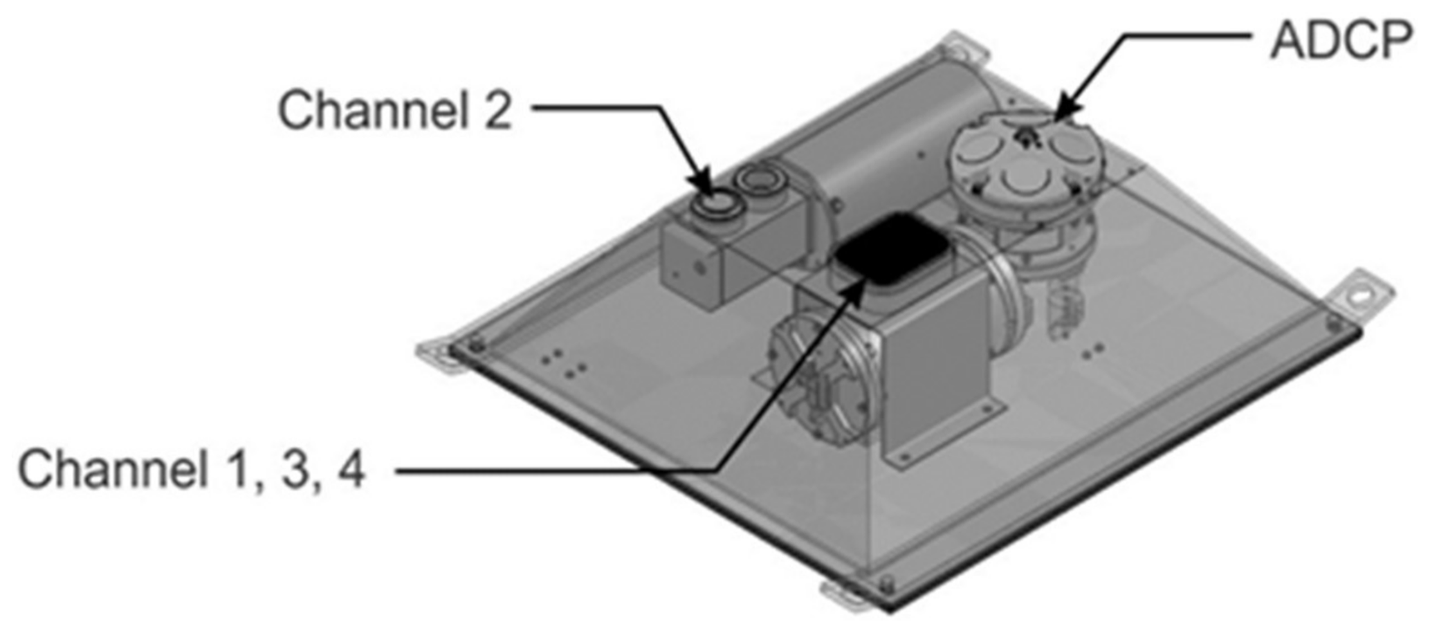
Figure 1The deployed instrument package showing the locations of the multifrequency SWIPS and ADCP current profiler including the locations of the SWIPS transceivers.
Individual acoustic pulses were transmitted and received in each channel at 1 Hz. Averaging over two adjacent time samples of the return voltage signals provided measures of backscattering from successive 4 cm range cells. Water temperature, hydrostatic pressure, flow speed, and direction profile data were acquired on a Teledyne RDI Sentinel acoustic Doppler current profiler (ADCP) included in the instrument package.
2.2 SWIPS measurement, data extraction, and model comparison methodologies
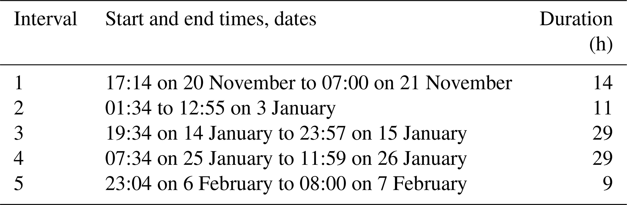
The analysis framework used in this work assumes availability of volume backscattering coefficient, sV, time series data at, at least, three different acoustic frequencies. Frazil characterizations utilized data averaged over contiguous 2 min time intervals during seven separate events spanning roughly 2.5 % of the 5-month SWIPS monitoring period. Detailed analyses were confined to four of five major supercooling events, listed in Table 1, which preceded seasonal ice cover consolidation at TPR.
Table 1Analyzed pre-consolidation frazil intervals. Times are given in Mountain Standard Time (MST).
Given the heavy reliance of river ice models on frazil ice volume, it was essential that the SWIPS-measured quantities, sV, be easily linked to volume-related parameters. This required access to a valid theoretical expression for sV expressible in terms of linear dimensions unambiguously convertible into scattering target volumes. In general terms, the required relationship can be written as
where N denotes the number of particles per unit volume; σBS(ae,νi) is the theoretical backscattering cross section of a spherical particle with an “effective radius” ae at an acoustic frequency νi; and g(ae) defines a probability distribution normalized to unity and expressed in a two-parameter lognormal form:
The effective radius, ae, is defined (Ashton, 1983) as the radius of an “effective sphere” having a volume equal to that of the represented particle. The two population parameters in Eq. (2), am and b, are, respectively, the mean value of the effective radius and the standard deviation of the logarithm of ae, which specifies the spread in the latter parameter. Given access to sV data acquired at, at least, three frequencies, population descriptions in terms of N, am, and b are obtained by minimizing a residual quantity, q, defined as the sum over all channels of squared differences between measured and theoretical logarithmic backscattering coefficients SV≡10log (sV):
The optimal population parameters allow fractional ice volumes to be calculated from
Valid measurements of F and extraction of other frazil information require the applicability of Eq. (1) and confidence in the cross-sectional relationship, σBS(ae,νi). The Marko and Topham (2015) testing established the validity of linear dependences on numerical target concentrations to values of N up to and, often somewhat above, 107 m−3. The FEST cross sections (Faran, 1951), σBS(ae,νi), can be expressed compactly in terms of modal series coefficients, ηm, (Stanton, 1989) as
Actual cross-sectional calculations utilized the formulation developed by Dezhang Chu of the Northwest Fisheries Center. In logarithmic terms, the formulation's accuracy was estimated to be better than 0.001 dB. Target-shape-related deviations from FEST cross sections, which appear as k1ae values approach roughly 0.45, required an additional corrective step suggested by the Topham and Marko (2020) validations to assure F(t) accuracies comparable to the ±30 % levels achieved in transducer calibrations.
Conversion of SWIPS sV outputs from three channels into frazil population parameters was carried out with ASL Environmental Sciences' RUNSWIPS software based upon FEST representations of the relationship between backscattering cross sections and the key acoustic frequency and effective radius parameters. Time series of F, N, am, b, and q values for each successive averaging interval were extracted and displayed (Marko et al., 2015) as functions of time at multiple, user-specified, heights in the water column relative to the common transceiver surface plane. Although variations in all frazil parameters provide important information relevant to suspension dynamics, the principal interests in the present work lie in the magnitudes and time dependences of F(t) at mid-water ranges. Detailed studies by Marko et al. (2015) and Topham and Marko (2020) suggest that values obtained for this parameter are robust and – when multiplied by 1.25 to account for higher-order, shape-related refinements of the FEST cross-sectional relationship – yield accurate F(t) estimates suitable for comparisons with model-simulated water-column-averaged F(t) values.
An essential component of the study involved interpretation of echogram plots of raw backscattered digital voltage signals (in counts) as recorded for returns from successive emitted acoustic pulses. The colour-coded strengths of these returns were displayed by ASL's ProfileView software as functions of the ranges of the scattering targets relative to the transducer faces.
The extracted F(t) time series were compared with simulations derived from runs of a one-dimensional CRISSP1D model (Shen, 2005) within BC Hydro's operational mode (Jasek et al., 2011) without further adjustments. These runs utilized inputs of water temperature and discharge data, available at hourly intervals at a hydroelectric site approximately 370 km upstream of the SWIPS instrument. Hourly surface air temperature inputs were obtained near river gauges 7 and 100 km downstream of the SWIPS location as well as 94, 226, 278, and 362 km upstream. The model utilized a 30 min time step and linear interpolations of hourly input data to produce corresponding water-column-averaged F(t) values. Detailed discussions of simulation procedures are available in Jasek et al. (2011).
3.1 Outline of analytical approach
Five separate intervals of supercooling and frazil growth were identified in the period (Table 1) separating the first appearances of frazil ice in late November 2011 from mid-February 2012 consolidation at the TPR monitoring site. The ice conditions which evolved during these intervals were reviewed for insights into the processes underlying seasonal ice cover development. Significant differences were apparent in the magnitudes and time dependences of the extracted frazil fractional volume parameters and in their correlations with blockages of acoustic beams. The latter phenomena and consequent gradual losses of frazil monitoring capability were interpreted as unmistakable evidence of anchor ice accumulation on or near exposed transceiver faces. Understanding the underlying growth processes required merging acoustic data and observations with external information (river and atmospheric environmental data) to provide a basis for a self-consistent interpretative model of frazil events.
In doing this, it was convenient to focus on the four most intense and persistent frazil events observed during the, roughly, 2-month period preceding local ice cover consolidation. These events were divided into two categories, primarily, on the basis of notable differences in the time dependences of the deduced parameter, F(t). The simpler generic form consisted of a single large peak at the beginning of the frazil interval followed by a sharp drop and stabilization at lower levels of frazil content. A March 2012 interval of this type was employed in the Topham and Marko (2020) SWIPS verifications. The two frazil intervals in this category studied here were closely spaced (in time) and dominated a late January–early February period preceding local consolidation. Although not necessarily associated with all intervals of this type1, both intervals were terminated by gradual decreases to negligible levels of frazil content attributable to anchor-ice-growth-related blockage of the acoustic beams. A second pair of intervals, corresponding to the alternative “multi-peaked” form, was encountered in late November and mid-January during the coldest portions of the pre-consolidation period. As indicated by the nomenclature, corresponding F(t) data featured multiple sharp peaks separated by periods of low or intermediate frazil content. In contrast with single-peak events, these intervals were terminated by disappearances of frazil in the water column without evidence of acoustic beam blockage.
Data on events in each category are analyzed separately in Sect. 3.1.1 and 3.1.2 to identify and quantify the processes controlling, respectively, the single- and multi-peak forms of frazil variations. This information provides a principal basis for understanding and modelling key initial steps in seasonal ice cover growth.
3.1.1 Single-peak frazil growth intervals
Frazil fractional volumes during the intervals of 07:34 MST (Mountain Standard Time) on 25 January to 11:59 MST on 26 January (interval 4) and 23:04 MST on 6 February to 08:00 MST on 7 February (interval 5) are plotted in Fig. 2a and b as derived from 2 min averaged sV data acquired in SWIPS channels 1, 3, and 4. The plotted results, representative of returns from frazil positioned roughly 2.3 m above the transceiver faces, exhibit the classic single-peak form and are terminated by acoustic beam blockages. The timings and intensities of the observed blockages, interpretable as two separate obstruction events, are summarized in Fig. 3 in terms of representations of coarse blockage severities as a function of time at each acoustic frequency. Three severity categories are delineated: unblocked, partially blocked, and completely blocked. Partial blockages occurred during transitions between the unblocked (unobstructed) and completely blocked (no returns from the water column or above) extremes. Additionally, in both events, blockage progress included partial daytime clearances prior to resumption of approaches to the full blockages achieved in later, evening or early morning, hours.
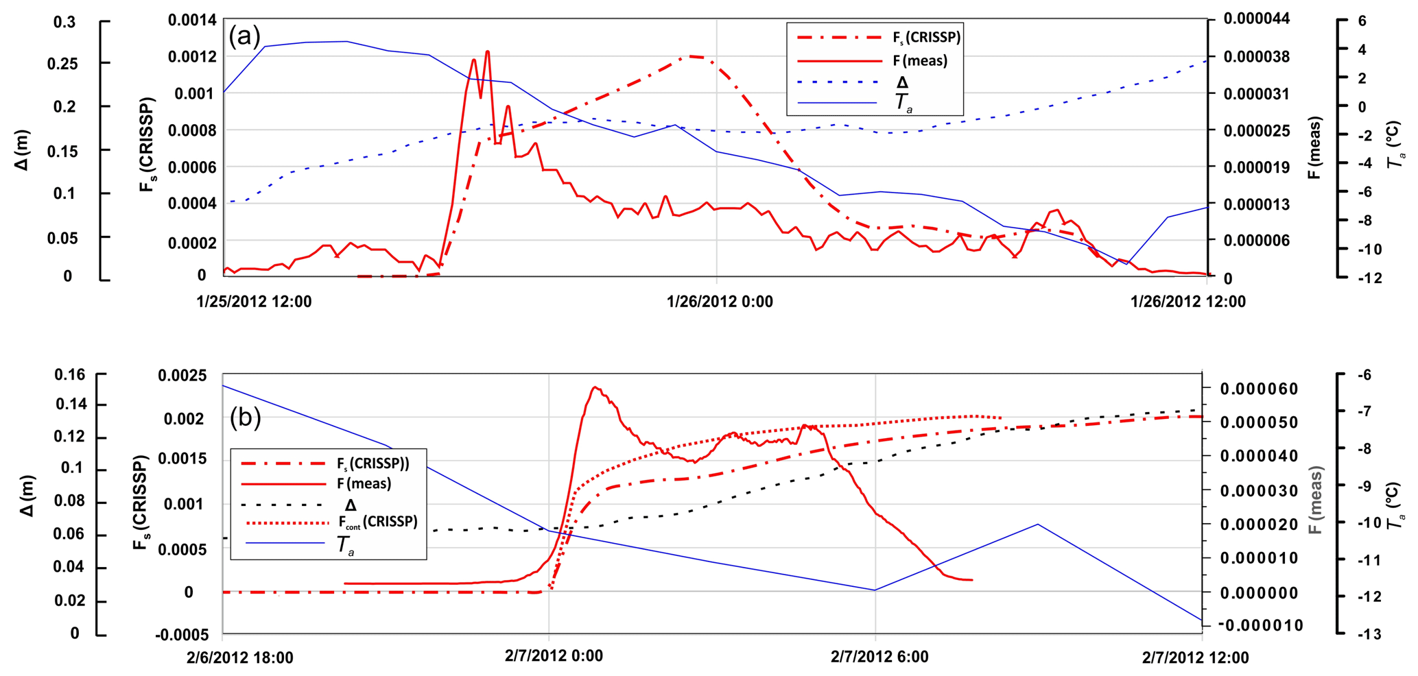
Figure 2Comparisons of fractional volumes as measured (F(meas)) and simulated (Fs(CRISSP), Fcont(CRISSP)) and Ta for (a) interval 4 and (b) interval 5. The Fs(CRISSP) simulations were shifted to earlier and later times by 11.0 and 3.5 h, respectively, to facilitate coincidence with observed frazil onsets. The plot in panel (b) includes Fcont(CRISSP) depicting an artificially triggered simulation described in the text which uses fully contemporary post-onset environmental inputs. The measured and simulated fractional volumes were representative of, respectively, measurements 2.3 m above the SWIPS instrument and water column mean values. An additional, dotted, curve in panel (b) represents Δ, the difference between 10-point-averaged measured water levels and those simulated by CRISSP1D without allowances for anchor ice. Model air temperature inputs, Ta, are plotted in both figures.
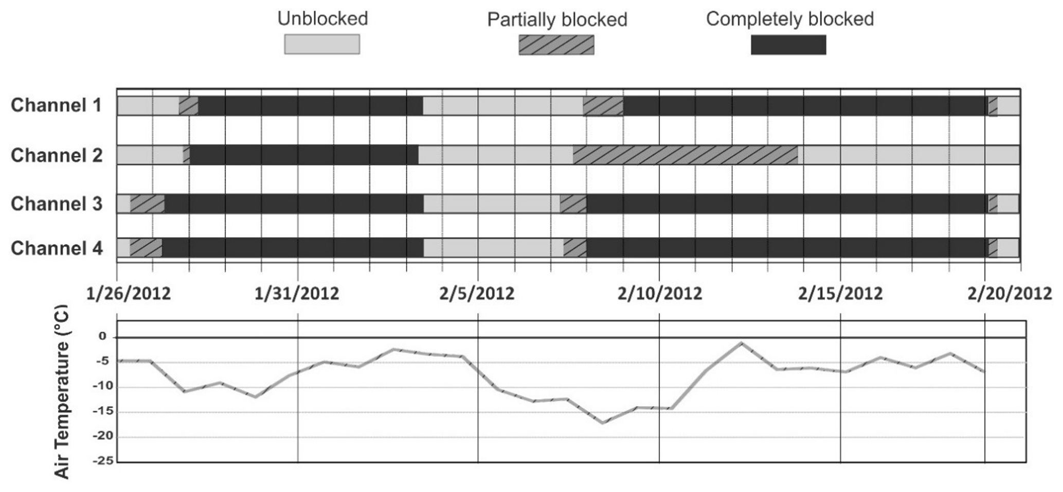
Figure 3Mean daily air temperatures at a gauging station 7 km downstream from the SWIPS and the timings of observed acoustic beam blockages during the 26 January–20 February 2012 time period. Temperature data extend up to and just beyond the upstream advance of the ice edge past the SWIPS site. Uncertainties in blockage transition timings were greatest (±2 h) at the starts and ends of partial blockages. Brief periods of partial blockage embedded in the completely blocked periods were not included in the plots.
The first onsets of the blockages in these events occurred 15 and 6 h after the initial appearances of water column frazil, which always preceded blockage occurrences. Except for a 3 d February period separating the two events, data included in Fig. 3 showed mean daily temperatures remaining close to or below, roughly, −5 ∘C for times as late as 19 February when the consolidated ice edge was established 3 km upstream of the SWIPS. Apart from the anomalous persistence of problematic channel 2 returns in the February interval, blockages were both first detectable and complete in the highest-frequency channels 3 and 4 but eventually encompassed all channels. Near-simultaneous clearances of the interval 4 blockages on 3 February were followed by the additional sequences of frazil formation and varying and, ultimately, complete blockage during frazil interval 5 (Fig. 2b). Again, in the latter case, blockages in all channels ended near-simultaneously on 20 February.
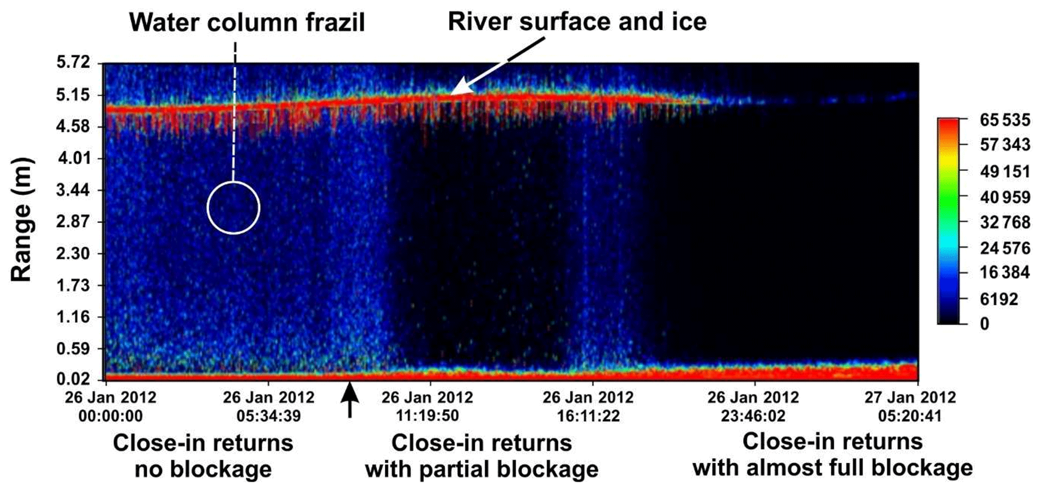
Figure 4Echogram of the channel 4 (774 kHz) returns during the first blockage event. The vertical arrow below the time axis denotes the approximately 08:00 MST start of the thickening of the close-in returns discussed in the text as indicative of transceiver blockage onset.
Figure 4 offers representative examples of changes in backscattering returns which allow tracking of frazil content and acoustic blockage development. The utilized echogram format provides false-colour mappings of 16 bit digital voltages representing acoustic returns in a given frequency channel as a function of time and range above SWIPS transceiver faces which are 29 cm above the riverbed. The plotted data, corresponding to 774 kHz (channel 4) returns, document scattering strength as a function of position in the water column during a key segment of frazil interval 4. The depicted period included progressive extinctions of returns from water column frazil and, eventually, from much stronger surface ice and atmospheric interface targets. Annotations denote echogram features relevant to interpreting changes during a period which began 7 h after the initial appearance of frazil in the interval. F(t) data for the full interval are plotted in Fig. 2a. Particular note is made in Fig. 4 of the narrow strip of “close-in” returns at the lowest end of the range scale. At times prior to, approximately, 08:00 MST on 26 January, this feature's very high digital count values were representative of transceiver “ringing” which persists for a brief period following each emission of a sound pulse. Subsequent progressive thickening of this strip was due to the buildup of anchor ice on and/or just above the transceiver faces. The first evidence of such ice is detectable as a slight but persistent elevation in the feature's upper boundary (beginning at a time roughly coincident with the vertical arrow in Fig. 4). The effects of such accumulations were more apparent, at approximately 10:00 MST on 26 January, in the onset of very visible weakening in the strength of returns from water column frazil. Smaller concurrent reductions were apparent in the longest-range components of the saturated surface returns. Blockage impacts and the width of the close-in zone began to decrease again at, roughly, 12:00 MST. This decrease eventually allowed recovery of water column frazil returns until 18:00 MST, when strong growth again widened the close-in regime, eliminating returns from the water column and rapidly eroding river surface signals. No surface or water column returns were detectable by early morning 27 January. Similar sequences were observed in connection with frazil interval 5, in which, as noted above, initial signs of acoustic blockage followed frazil onset by 6 h.
A common pattern was noted in which changes in the strengths of returns from water column frazil and surface targets were closely correlated with and opposed in sign to contemporary variations in the spatial extent of strong close-in returns. As suggested above, these correlations were consistent with anchor ice presence adjacent to the transducer faces in volumes large enough to partially and, later, completely block detection of acoustic returns from water column and surface targets. A second, more practical, inference was that such sudden appearances of anchor ice above a heated transceiver surface, almost 30 cm above the riverbed, imposed an additional, potentially useful, constraint on river ice models. Specifically, such models had to incorporate frazil and anchor ice relationships which were compatible with this and other observations made in the water column and near the riverbed during the 2011–2012 studies.
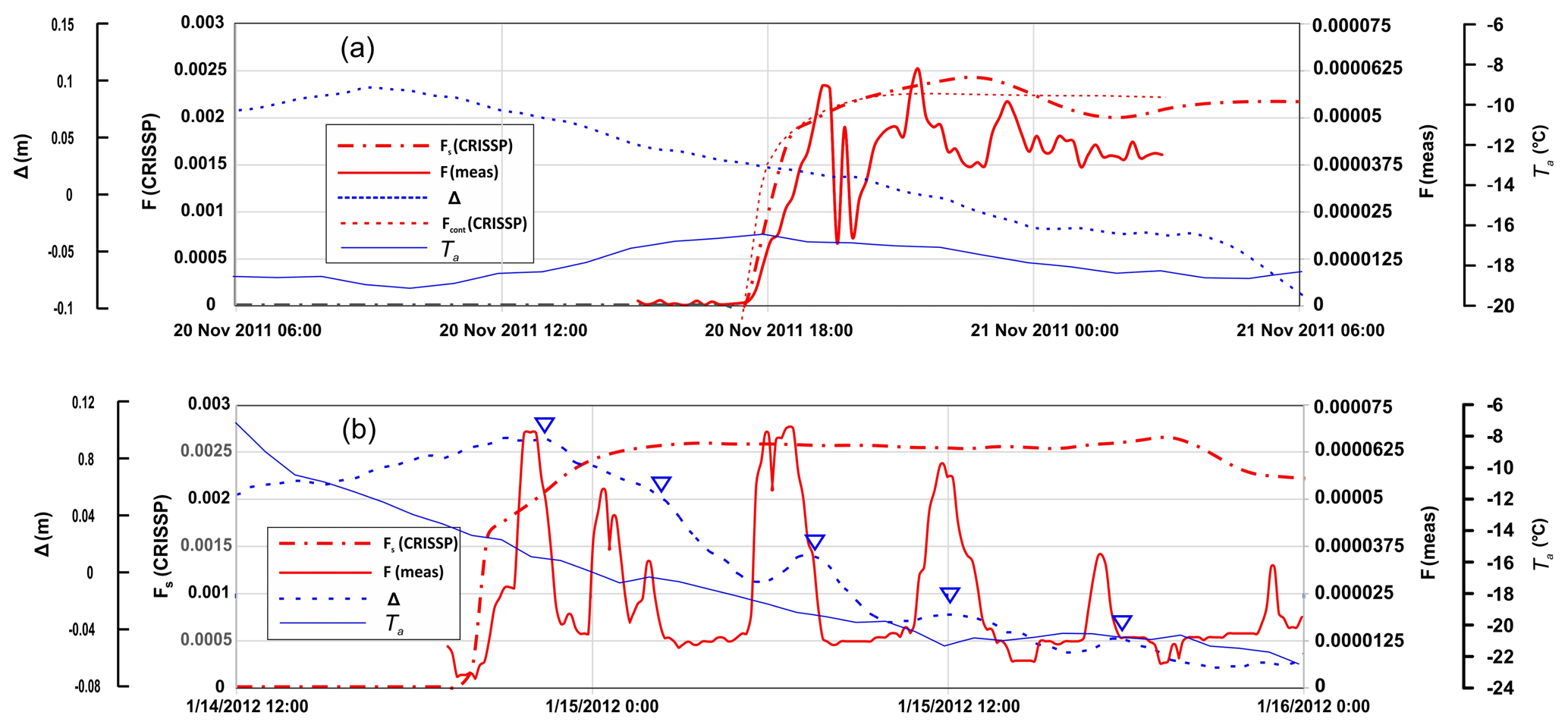
Figure 5Comparisons of fractional volumes as measured (F(meas)) and simulated (Fs(CRISSP), (Fcont(CRISSP)) for (a) interval 1 and (b) interval 3. The Fs(CRISSP) plots were shifted to later and earlier times by 12.65 and 15 h, respectively, to facilitate coincident simulated and measured frazil onsets. The plot in panel (a) also includes Fcont(CRISSP) depicting an artificially triggered simulation described in the text based upon fully contemporary post-onset environmental inputs. The measured and simulated fractional volumes represented, respectively, regions 2.3 m above the SWIPS instrument and water column mean values. The additional, dotted, curves represent Δ, the difference between 10-point running-average local water levels and levels simulated by CRISSP1D in the absence of anchor ice. The inverted triangles in panel (b) denote the central positions of anomalous anchor-ice-related water level peaks. Model air temperature inputs, Ta, are also plotted in the figures.
Immediate insights into such relationships were available from further use of the above-noted Osterkamp (1978) thermodynamic approach previously employed (Ye et al., 2004) to estimate frazil fractional volumes in a laboratory flume. In our case, it was appropriate to initially focus on the transition from frazil-free to frazil-infested conditions, assuming frazil onset to be accompanied by a rough continuity in the rate of sensible heat loss to the atmosphere. This assumption was consistent with the negligible, few-millidegree, initial warmings of the supercooled water column during early stages of frazil crystallization. In preserving continuity, the energy balance required that the initial rates of frazil latent heat production (derived from immediately post-onset F(t) data) had to be at least equal to pre-onset sensible heat fluxes. This equality was tested against the SWIPS-estimated rates of F(t) increase plotted in Fig. 2a and b and in the equivalent multi-peaked interval results of Fig. 5a and b. Pre-transition sensible heat fluxes, on the other hand, were calculated from the time rates of change in water temperatures measured on the ADCP instrument. These comparisons are made in Table 2 for both single- and multi-peaked intervals. Results for interval 4 were not included in the tabulation due to notable anomalies in corresponding pre-onset water temperature data which precluded reliable estimates of sensible heat loss rates. It can be seen that the ratios of post- to pre-onset fluxes for the three evaluated intervals were consistently an order of magnitude or more below unity. This result suggested that most of the heat lost to the atmosphere after frazil onset did not originate from frazil growth in the water column as assumed in anchor-ice-free CRISSP1D simulations (Shen, 2005; Jasek et al., 2011; Marko et al., 2015).
Table 2Comparisons of pre-onset sensible heat fluxes and post-onset fluxes of latent heat from frazil growth.

To help understand this point, the single-peak F(t) results plotted in Fig. 2 for intervals 4 and 5 are accompanied by corresponding outputs from anchor-ice-free CRISSP1D simulations similar to those reported previously (Jasek et al., 2011). As in the earlier work, these comparisons were necessarily limited by reliance (Sect. 2.2) on model inputs of water temperature data acquired 370 km upstream of the SWIPS monitoring site. Consequent differences in the timings of, respectively, the simulated and observed onsets of frazil growth ranged between 3.5 and 15 h for the documented 2011–2012 frazil intervals. Fortunately, it can be shown (Marko et al., 2017) that the close similarity of atmospheric conditions during the actual and the temporally closest significant simulated event still allowed meaningful comparisons. This approach simply shifted the simulated F(t) output ahead or back in time to bring the simulated and observed frazil onsets into coincidence. The resulting Fs(CRISSP) curves in Fig. 2a and b, thus, represented model inputs corresponding to times, respectively, 11 h later and 3.5 h earlier than indicated on the horizontal plotting axes. The second approach, applicable to simulations predicting premature (early) frazil onsets, artificially incremented the model's upstream water temperature inputs, Tw, for a short period sufficient to force simulated frazil nucleation into coincidence with the observed onset. For interval 5, this adjustment required a brief 0.25 ∘C temperature increase. This artifice ensured that all environmental inputs employed in producing the model output, Fcont(CRISSP) during the observed frazil event, were completely contemporary with the measured quantities, F(meas). Comparisons of the shifted, Fs(CRISSP), and contemporary, Fcont(CRISSP), curves in Fig. 2b confirm expectations that simulated F(t) magnitudes and time dependences were relatively insensitive to the precise timing of supercooling onset. This insensitivity reflected the reality that both simulated and observed frazil events are associated with extended periods of decreasing air temperatures. When two such periods are characterized, as in the case of the studied intervals, by similar average air temperatures, temporal shifts in the simulations, necessitated by millidegree errors in modelled water temperatures, have relatively minimal impacts on comparisons with measured fractional volume magnitudes and time dependences.
It is to be noted that the comparisons in Fig. 2a and b (and in Fig. 5a and b below) required use of Fs(CRISSP) and Fcont(CRISSP) plotting scales which are 40 times larger than those used to display F(meas) results. This difference was necessary to demonstrate the simulations' consistent tendency to overpredict frazil content by as much as 2 orders of magnitude. Specifically, the ratios of simulated to measured quantities ranged, roughly, between 50 and 150 over the course of interval 4. In interval 5, the 40-fold difference in the simulated and measured plotting scales was more consistently reflective of observed differences. Most importantly, the observed characteristic forms of the single-peak events – with initial sharp rises being followed by similarly sharp drops and lower, relatively constant, fractional volumes – were not anticipated by the simulations. Instead, the simulated rapid initial rises in fractional volume were followed by persistently high frazil contents. All these results supported the premise that model simulations which ignore anchor ice growth cannot be representative of observed Peace River frazil behaviour.
Possibilities for addressing this difficulty were explored by Jasek et al. (2011) based upon comparisons between measured surface ice parameters and their simulated counterparts as derived from CRISSP1D model runs which incorporated anchor ice growth. The lack of consistency in the obtained results combined with the apparent agreement achieved between a corresponding anchor-ice-free model and available surface ice data led to the conclusion that anchor ice was not a major factor in river ice cover growth. In retrospect, this conclusion was, in large part, a consequence of the model assumption that anchor ice growth occurred primarily by riverbed capture and accretion of water column frazil. The implicit neglect of alternative in situ anchor ice growth was fully consistent with a contemporary consensus (Daly, 2013) that such growth was confined to smaller, more slowly moving water bodies as opposed to larger “flowing rivers”. Nevertheless, the frazil capture mechanism was unable to produce anchor ice in the amounts required for compatibility with observed surface ice growth in the presence of frazil concentrations as low as those plotted in Fig. 2. On the other hand, the 1 m s−1 and larger velocities, typical of most rivers, would be expected to greatly enhance heat removal from riverbed-fixed ice crystals (Piotrovich, 1956) relative to free-drifting frazil. This difference favours in situ riverbed anchor ice production, specifically allowing the results in Table 2 to be interpreted as evidence that such production is the dominant source of latent heat input to the water column. In the best-documented interval, interval 5, the table results suggest that “missing” latent heat contributions from this source were equivalent to a solid ice layer thickening at a rate of 2.9 mm h−1. This estimate, and the underlying mismatch of sensible- and latent-heat fluxes, tells us much about the dynamics of the critical early stages of seasonal ice growth. Specifically, apart from being initially “seeded” by captured frazil crystals, riverbed anchor ice growth would appear to control the rate of frazil production and not the other way around as assumed in the Jasek et al. (2011) simulations.
Other, finer, details of the 2011–2012 acoustic data provided an important basis for expanding this conclusion into a quantitative interpretative model of ice processes in the water column. For example, the time delays separating the first onsets of frazil formation from subsequent initial signs of acoustic blockage offered a means for estimating riverbed ice layer growth rates prior to actual acoustic beam blockage. Additional information on these rates was also encoded in the time dependences of the close-in acoustic returns depicted in the echogram of Fig. 4. As noted above, the range spanned by these returns, which include contributions from backscattering by ice on or immediately above the transceivers, was observed to increase in concert with attenuation of acoustic returns from the water column and river surface. Such changes contained basic information on growth rates during later portions of the anchor growth cycle, yielding information on ice layer elements at elevations close to or above the SWIPS transceivers.
Studies of these more subtle aspects of the acoustic data were only feasible because of electrical heating of the instrument package. This heating was intended to assure instrument physical stability and profiling capabilities. The sudden losses of the latter capabilities several hours into intervals 4 and 5 were, initially, inexplicable. However, it was recognized that the above-cited thermodynamic evidence for anchor ice fractional volumes increasing at rates of several millimeters per hour offered a mechanism for explaining subsequent obstructions of acoustic beams transmitted from elevations 29 cm above the riverbed. Specifically, the 15 and 6 h delays separating the respective onsets of frazil in intervals 4 and 5 from subsequent first signs of beam blockage provided reasonable measures of the times required for the upper surfaces of growing riverbed layers of porous anchor ice to reach the transceiver faces. Consequent accumulation and “overspilling” of this ice layer onto and/or above the transceivers was likely to resemble behaviour previously reported by Qu and Doering (2007) for anchor ice produced by frazil capture in a laboratory flume. Given the transceiver elevations and the thermodynamically inferred 2.9 mm h−1 growth rate in terms of an equivalent layer of solid ice, these results suggested that, during at least the first 6 h of interval 5, an anchor ice layer with an approximately 90 % porosity was accreting at a rate of, roughly, 4.4 cm h−1.
The close-in return data also enabled quantifying still later stages of layer growth during which anchor ice was in contact with or above the SWIPS transceivers. This ice not only weakened or eliminated acoustic returns from water column frazil and surface ice but also contributed its own backscattered returns as a measure of blocking layer thickness. The parameter of quantitative interest was the extent to which the range spanned by the close-in feature was incremented above its minimal (baseline) value2 as observed prior to any weakening of water column acoustic returns. As seen in Fig. 4, such increments in close-in return width typically varied during a frazil event, with initial widening being reduced or eliminated during warmer mid-day hours before increasing again, accompanied by the fading and disappearance of water column and surface returns. Meaningful estimates of increments were only possible during periods associated with thickening of the close-in feature. (Such thickening confirms that acoustic pulses are still penetrating and, hence, sampling the full height of the close-in ice layer.) Our procedure estimated such range increments for portions of this feature having digital signal levels > 24 000 counts as a function of time after the first signs of return blockage. This treatment ignored the noted temporary decreases in close-in range span, presumably caused by melting and/or ice detachment. While probably underestimating actual thicknesses, the use of a moderately high-count threshold minimized possibilities for overestimating thickness by inclusion of late returns associated with multiple scattering (i.e. from returns along trajectories incorporating more than one scattering target).
Increments in the thickness of the close-in ice layer, Δr, were derived from corresponding increments in Δr′, the maximum range of associated signal returns. The latter quantities, which could be read off the zoomed-in echogram scale or extracted from the underlying digital data, required conversion to ice thickness with the simple relationship
where c1 and ca, respectively, denote the speeds of sound in freshwater and anchor ice at 0 ∘C. Reasonable minimum estimates for ca equal to 1000 and 1200 m s−1 were available, respectively, from earlier laboratory and Peace River field measurements on slush ice (Marko and Jasek, 2010a). A more robust, if less relevant, extreme upper limit was given by the 3840 m s−1 value measured by Vogt et al. (2008) in bubble-free zero-porosity ice. Using these results to set 1000 and 1800 m s−1 as possible lower and upper bounds of anchor ice sound speed, it was convenient to set ca=c1, allowing Δr and, hence, close-in thicknesses to be read directly off echogram plots. This assumption was consistent with the high porosity deduced above from the timings of blockage onsets, giving tolerable ±30 % uncertainties in thickness estimates. To minimize complications from wavelength-sensitive near-field effects and transducer ringing, thickness estimates were derived from data acquired at the highest acoustic frequency, 774 kHz (channel 4), characterized by the smallest ranges spanned by close-in returns prior to blockage onset. The plotted results (Fig. 6) showed detectable accumulations reaching 23 and 14 cm during, respectively, the first and second blocking events. Roughly similar, 3–4 cm h−1, growth rates characterized the initial stages of both events, which preceded temporary clearances, consequently offering the best measures of fundamental layer thickening rates. Thus, at least prior to thicknesses becoming large enough to rule out further measurements, layer growth rates at levels ≥ 30 cm above the riverbed were comparable to those inferred above from earlier stages of frazil and anchor ice growth.
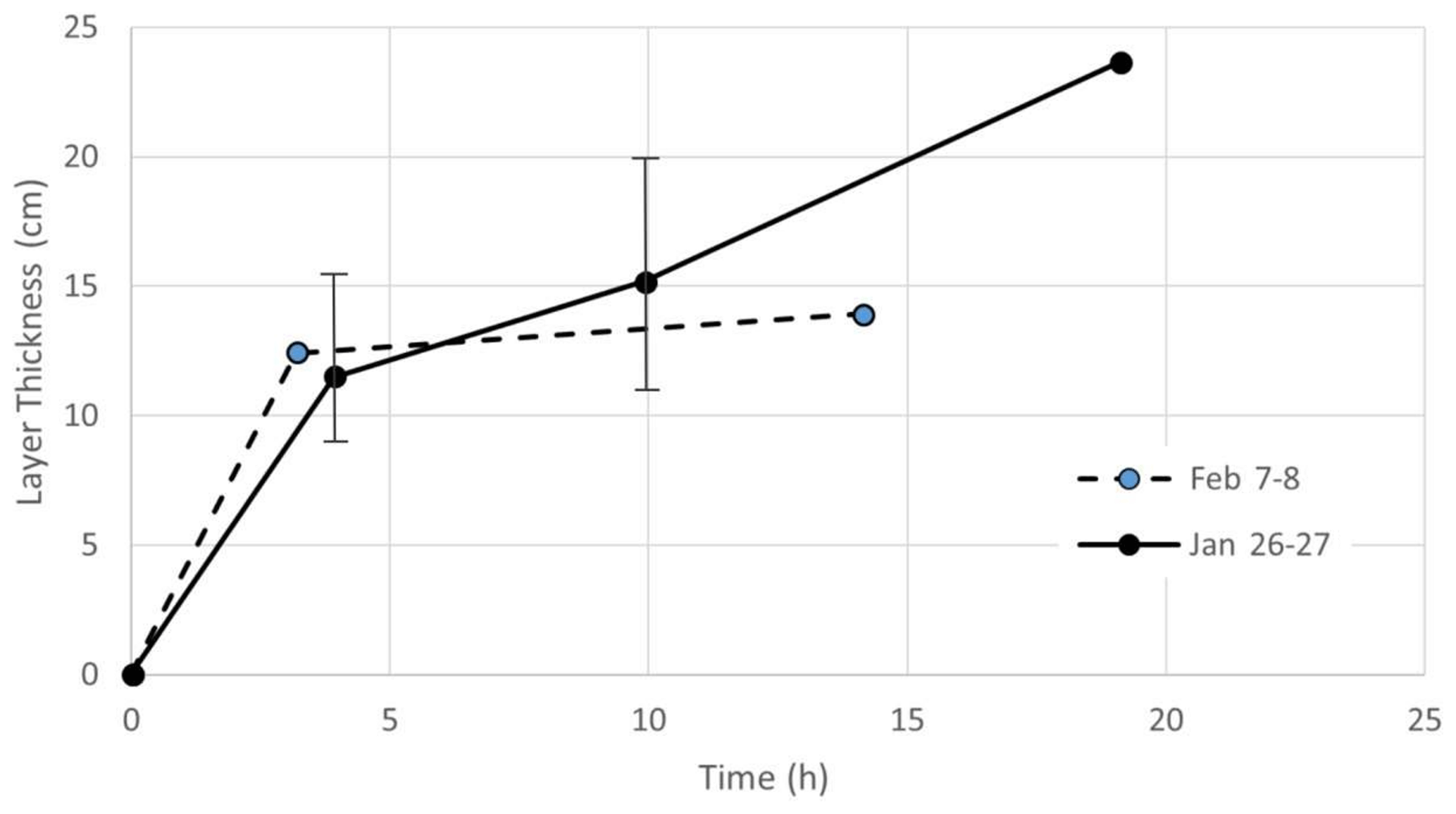
Figure 6Estimates of anchor ice accretion above the elevated SWIPS transducers during the 26–27 January and 7–8 February blockage events as a function of time since event onset. The 26–27 January error bar data are representative of both intervals.
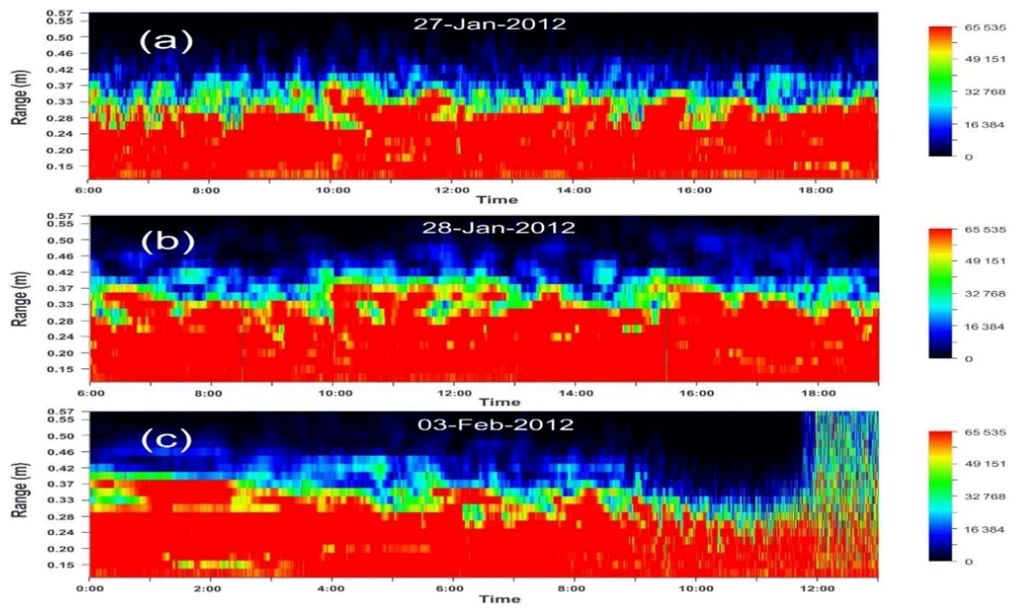
Figure 7Zoomed-in channel 4 close-in returns acquired during 13 h intervals at different stages of the interval 4 blockage event. Panels (a) and (b) depict intervals initiated at times coinciding with complete extinctions in, respectively, the high-frequency (06:00 MST, 27 January) and low-frequency (06:00 MST, 28 January) channels, roughly 24 and 48 h into the interval. Panel (c), initiated at 00:00 MST on 3 February, terminates with a blockage-ending ice clearance event.
Evidence was also acquired suggesting significant growth occurred at layer thicknesses which exceeded those plotted in Fig. 6 but which could not be quantified due to incomplete acoustic penetration of still higher ice layer levels. Instead, zoomed-in returns from ranges within, roughly, 0.5 m of a transceiver face showed (Fig. 7) that the inferred continuation of growth over periods of several days produced systematic changes in the temporal and spatial spectra of returns from the lower, insonified, portions of the ice layer. Such changes, consistent with continued layer growth, are illustrated in successive panels representing data from three 13 h periods acquired at 24 h intervals. The panels show significant initial increases with time in the size of image features sharing common levels of return signal strength. This trend toward greater homogeneity was suggestive of increasing ice layer stability. In the final third of the last panel, high-frequency variations suddenly reappeared, presaging the imminence of an observed layer clearance.
Additional single-peak analyses were carried out to quantify connections between in situ frazil growth and environmental forcing relevant to later interpretations of multi-peak data in Sect. 3.1.2. Results obtained during interval 5 were of particular value in offering a basis for identifying thermodynamic requirements for anchor ice growth sufficient to initiate acoustic blockage. A critical feature of this interval was that it was immediately preceded by 72 h of undetectable water column frazil during a period in which simulated and ADCP-measured water temperatures rose as high as 1.1 and 0.5 ∘C, respectively. Under such conditions, subsequent growth of an anchor ice layer could be assumed to have begun on a completely ice-free riverbed at the observed, 23:30 MST on 6 February, onset of frazil growth. Consequently, the 6 h delay separating this onset from the first detectable signs of acoustic blockage offered a means of establishing a minimum cumulative heat flux requirement for producing the 29 cm layer of 90 % porosity ice postulated above to have initiated beam obstruction. CRISSP1D cumulative heat fluxes, Φ, were calculated for the unblocked portion of the frazil interval using contemporary atmospheric and water temperature inputs, Ta and Tw, and a linear proportionality between Φ and water–air temperature differences. This flux can be expressed as
where Ci represents surface ice coverage and K=17 W m−2 denotes a proportionality factor established by Shen et al. (1984) from optimal matching of modelled and measured surface ice parameters. It was found that onset of blockage required a cumulative flux of 5.6 MJ m−2.
Additional information on river and ice conditions was available from hydrostatic pressure measurements made on the ADCP instrument. Unfortunately, connections between riverbed ice and the derived water levels are, generally, ambiguous, especially in large regulated rivers subject to multiple sources of variability. Anchor ice impacts on water levels, arising from changes in effective river cross section and bed roughness, can be of either sign, depending upon the stage and the positioning of the ice growth relative to the measurement site (Kerr et al., 2002; Jasek et al., 2015). In the Peace River studies, ice effects were documented by comparisons of measured water levels with expectations from completely ice-free CRISSP1D simulations, which included corrections for flow travel times and attenuation of regulated dam discharges. The ice-related water level changes, plotted in Fig. 2a and b, show that onsets of the two single-peak intervals roughly coincided with the beginnings of slow, sustained level rises. The interval 4 increase peaked at 0.6 m (Marko et al., 2017) just prior to the 3 February clearance event (Figs. 3 and 7), significantly higher than the 10 to 20 cm increases associated with earlier frazil events.
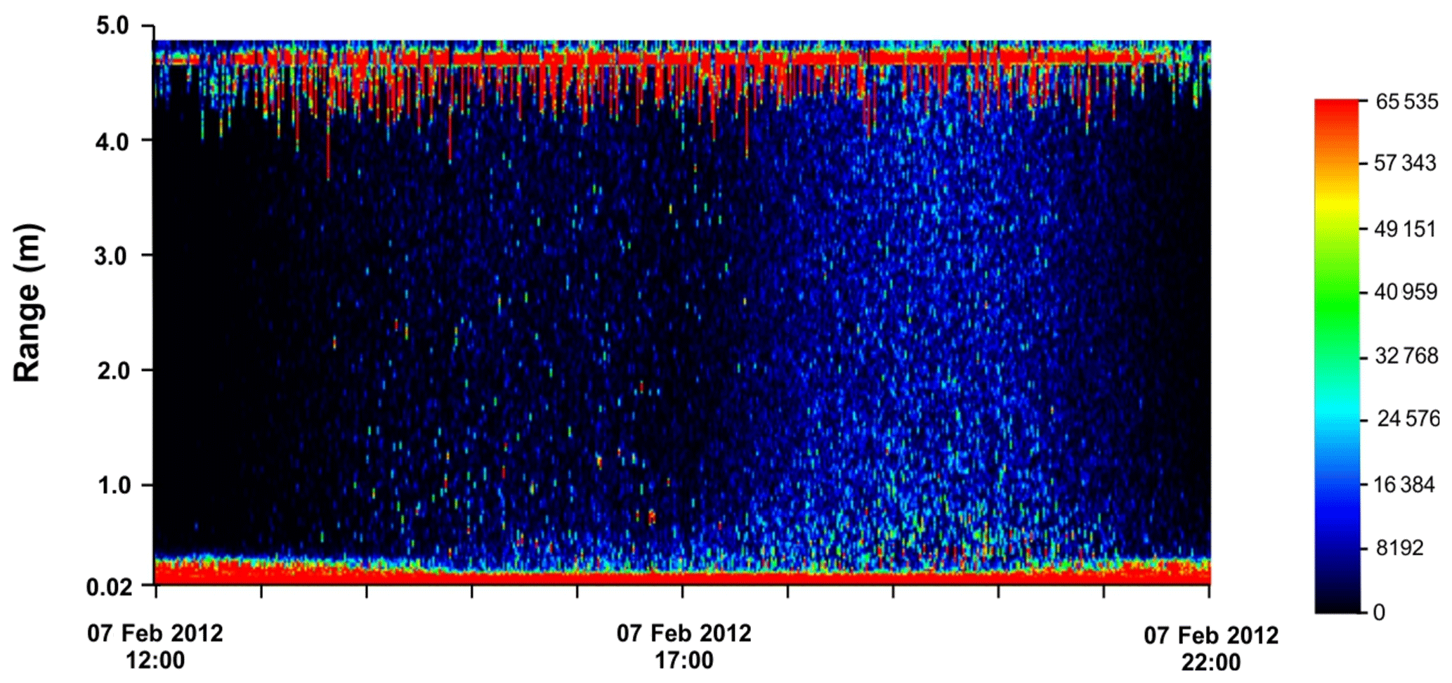
Figure 8Echogram of the channel 4 (774 kHz) returns at times subsequent to the measurements underlying the interval 5 F(t) data in Fig. 2b. The plotted return strengths show that the, roughly, 14:00 MST thinning of the close-in feature, indicative of anchor ice clearance, is shortly (15:00 to 17:00 MST) followed by both initial appearances of weak frazil returns and small numbers of high-intensity returns, consistent with anchor ice fragments produced by the upstream clearing process.
Taken together, these independent and relatively coarse characterizations of riverbed ice formation suggest that anchor ice grown in situ is the most influential subsurface ice species in the Peace River. In this view, the most important function of water column frazil is to provide seed crystals which adhere to the riverbed, initiating in situ anchor ice growth and its accompanying latent heat production. The latter heat reduces frazil growth below levels anticipated in the absence of such growth. In single-peak events, frazil production is largely confined to a relatively short-lived burst of initial growth followed by establishment of quasi-equilibrium conditions at much lower frazil content levels as determined by the latent heat output of contemporary in situ anchor ice growth. Frazil fractional volumes begin to fall at the ends of the plotted sequences (Fig. 2), due to onsets of beam blockage. Relatively brief reversals of the blockage process, triggered by diurnal variations in energy exchanges with the atmosphere, are common (Fig. 4), allowing release of anchor ice fragments and upward movement to the river surface. Acoustic detection of such fragments requires identifying isolated echogram pixels associated with anomalously strong returns. In the Peace River, these fragments are, typically, moving downstream at 1.25 m s−1 and, thus, rarely linger in the relatively narrow SWIPS sampling volumes over the 1 s time interval separating successive pings. Fragment detection is illustrated in Fig. 8 by echogram data from the period of 12:00–22:00 MST on 7 February associated with a diurnal clearance of the temporary blockage which terminated the frazil interval (interval 5), depicted in Fig. 2b. The period of coverage in the Fig. 8 begins with the thinning of the close-in return signals indicative of anchor ice clearance and the consequent progressive reappearance of surface returns. Gradually (around 15:00 MST) the faint light blue signatures of suspended frazil reappear and strengthen, accompanied, in the lower water column, by scattered single ping returns exhibiting the green-to-red coding indicative of much stronger, non-frazil, ice objects. It is to be noted that detached fragments are not detectable in F(t) plots which incorporate time averaging and represent returns from specific fixed mid-water-range cells. Video evidence of actual detachment and downstream drift of anchor ice sheet fragments has been reported by Jasek et al. (2015).
3.1.2 Multi-peaked frazil growth intervals
The results presented in Fig. 5a and b for the November and mid-January intervals 1 and 3 offered striking contrasts with the above-described single-peak behaviour. Differences included both the oscillatory multi-peaked form of F(t) and a tendency for water levels to peak at or shortly before frazil onset and, subsequently, decrease. Mean air temperatures for these two intervals, −18 and −20 ∘C, were significantly below those, −6 and −15 ∘C, associated with intervals 4 and 5. Again, the limitations of CRISSP1D input data required comparisons which shifted simulated F(t) outputs 12.6 h back and 15 h forward, respectively, for intervals 1 and 3 to force coincident simulated and observed frazil onsets. As in interval 5, a premature simulated onset of interval 1 allowed a brief artificial, 2.1 ∘C, increase in model upstream water temperatures to effect comparisons of F(meas) with fractional volumes,Fcont(CRISSP), simulated with fully contemporary environmental data.
Again, simulations neglecting anchor ice production can be seen to have failed to capture both the magnitudes and qualitative character of the observed frazil variations. The colder air temperatures accompanying multi-peaked events appeared to increase the peak magnitudes of frazil fractional volume by, roughly, 20 % relative to single-peak intervals. However, the principal impact of lower temperatures was to introduce additional strong F(t) peaks separated by periods of relatively steady lower frazil contents. In all cases, frazil contents, again, fell short of simulation expectations by more than 1 order of magnitude.
This behaviour readily lends itself to interpretation in terms of the in situ anchor ice growth model developed above to account for single-peak behaviour and acoustic blockage occurrences. In fact, it is not unreasonable to anticipate that much of the distinction between the two generic frazil interval types can be attributed to differences in the external environmental energy exchanges which control growth of riverbed ice and its subsequent upward transport to the river surface. Exploring this possibility can draw upon two important pieces of information: namely, (1) that acoustic blockages were not observed during the multi-peaked frazil intervals and (2) that frazil growth sufficient to initiate acoustic blockages was estimated above to require cumulative fluxes of, at least, 5.6 MJ m−2. The latter requirement explains the absence (Marko et al., 2015) of blockages during an additional 6 h, single-peaked, frazil interval (interval 2 in Table 1) during which the accompanying cumulative flux over the full interval (calculated using Eq. 7) was only 2.8 MJ m−2. Similar absences during the multi-peaked intervals 1 and 3 coincided with air temperature ranges of −16.5 to −19 and −14 to −22 ∘C, respectively. Cumulative heat flux calculations indicated that, at such air temperatures, exceedance of the estimated 5.6 MJ m−2 blockage threshold would have occurred 5.2 h (interval 1) and 4.7 h (interval 3) after anchor ice growth resumed following the terminations of the initial F(t) peaks in these intervals. However, the observed appearances of additional frazil peaks 3.7 and 4 h, respectively, after the initial peaks suggest that the anticipated acoustic blockages had been preceded by new clearances and transports of released anchor ice to the river surface. The latter releases would have short-circuited the ice layer buildup at thickness values below the threshold required for initiating acoustic blockage. The observed additional peaks were, thus, markers of re-accelerated frazil growth stimulated by the lower rates of latent heat production associated with recently depleted anchor ice layers. In this interpretation, the multi-peak structure of frazil events is a consequence of alternating intervals of layer growth and clearance controlled by the time-dependent physical stabilities of rapidly growing riverbed ice layers. The results suggest that, in intervals 1 and 3, layer growth tended to vary drastically on temporal scales shorter than the 6 and 15 h periods required to initiate acoustic blockages in intervals 4 and 5, respectively.
The implied differences in the stabilities of riverbed ice during the alternative single- and multi-peaked varieties of frazil intervals are most easily explicable in terms of ice layer stabilities being very sensitive to the air temperatures accompanying layer growth. This possibility was first suggested by Parkinson (1984), who identified physical differences between anchor ice grown at, alternatively, air temperatures in the −5 to −10 ∘C range and near −20 ∘C. More recently, Dubé et al. (2013) explicitly noted that the physical stabilities of ice dams containing anchor ice tended to increase when grown during multiple intervals of modest cooling as opposed to single episodes of “hard” freezing conditions. It is, thus, to be expected that in the latter case – i.e. layer growth at air temperatures below, very roughly, −15 ∘C – a riverbed ice layer is much less likely to remain in place relative to one grown at higher temperatures (“soft” freezing conditions). This situation is schematically depicted In Fig. 9.
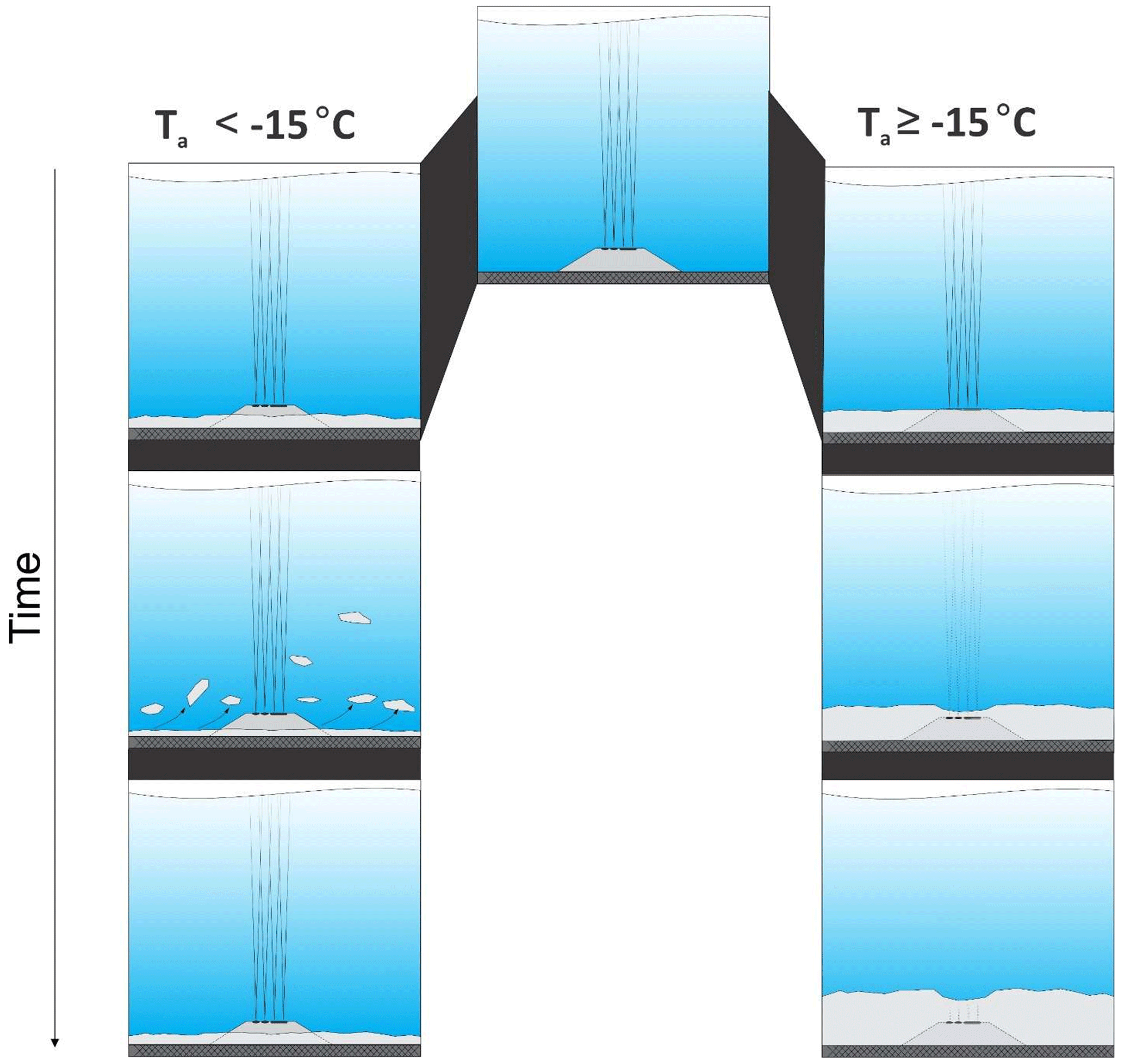
Figure 9Schematic illustrations of impacts on SWIPS profiling of the proposed anchor ice layer evolution mechanism (with time advancing downward) under alternatively soft ( ∘C) and hard ( ∘C) supercooling conditions.
Nevertheless, aside from differences in the relative stability of the respective anchor ice layers, distinctions between single- and multi-peaked frazil events may still be possible, within our limited database, in terms of the opposing signs of the water level changes during frazil growth. Thus, the steady decreases noted in ice-related water level displacements, Δ(t), during both multi-peaked intervals (Fig. 5a, b) ran directly counter to the rising trends noted during single-peak intervals (Fig. 2a, b). Interpretations of these differences are complicated by the above-noted sensitivities of local water level responses to riverbed conditions, stages of ice cover development, and measurement locations (Kerr et al., 2002; Jasek et al., 2015). A possible exception to this complexity was observed during interval 3 in the form of weak but detectable peaks in Δ(t) which consistently appeared to coincide with the downslopes of F(t) peaks. This timing was compatible with the above interpretations of oscillatory fractional volume behaviour and could be taken as evidence of the re-starting of “new”, hydraulically “rough”, anchor ice growth (Kerr et al., 2002) following partial or complete layer clearances. The latent heat produced by this new growth would have already reduced supercooling enough to force reductions from the immediately preceding fractional volume peak, and continuing growth could have smoothed the new ice layer topography, eliminating the observed initial brief increases in Δ(t). Efforts to test, modify, or replace such a hypothesis may be hard to justify given the brevity and magnitude of the effect and its confinement to a single frazil interval roughly coincident with the seasonal air temperature minimum.
4.1 Summary
The results presented above were based upon data acquired during a single annual field program in one river. Given the central role of numerical river ice models and, specifically, the CRISSP1D model, in the river management, a primary goal of the original underlying data collection and analysis was model “calibration”. It soon became apparent that the quality and breadth of the acquired data allowed more than fine tuning of model parameters. Specifically, measured peak frazil fractional volumes were, at least, 40 to 50 times smaller than inferred from model interpretations of surface ice data. Moreover, while high fractional volumes were anticipated throughout the durations of frazil events, estimated values were usually about 50 to 80 % below levels attained in brief periods of maximal content. Data on the timings and volumes of instrument ice accretion and consequent losses of profiling capabilities were recognized to be accidental, but essential, inputs for understanding deviations from expectations.
Progress in these regards utilized a simple interpretative model which assumed that supercooling triggers near-simultaneous production of frazil in the water column and significantly stronger in situ growth of anchor ice on the riverbed. The latter growth is, almost certainly, initiated by relatively small numbers of frazil crystals which previously impact upon and adhere to the riverbed. This situation reflected the large disparities in the rates of turbulent heat dissipation at surfaces of, alternatively, free-drifting and static, bottom-affixed frazil crystals. The larger relative water flow velocities in the latter case made the riverbed the principal site of sub-surface ice production. Thermodynamic data and SWIPS measurements of frazil fractional volumes suggested that – in the initial, most intense, portion of a frazil event – riverbed ice mass growth exceeds water column frazil mass production by more than an order of magnitude. Given this disparity and the resulting dominant influence of latent heat production by anchor ice on water temperatures, it is not surprising that river models neglecting in situ growth greatly overestimate frazil concentration. Frazil variations closely track changes in the riverbed ice layer.
Although it was convenient to separately consider frazil intervals characterized by two apparently different generic forms of temporal variability, it was eventually concluded that this distinction was, primarily, a consequence of differences in the physical stabilities of the contemporary anchor ice layers. In spite of the small number of analyzed intervals, our results and prior observations by other workers (Parkinson, 1984; Dubé et al., 2013) suggest that layer stability decreases proportionately with increasing cooling rates. Specifically, air temperatures below −15 ∘C appeared to favour growth of unstable ice layers, allowing repeated rises and falls (i.e. peaks) in water column frazil content above comparatively stable baseline levels. These peaks follow partial or full clearances which initiate buoyancy-driven movements of high-porosity anchor ice to the river surface.
Estimates suggest that per unit area production of anchor ice was equivalent to a solid ice layer thickening at a rate of approximately 3 mm h−1. This accretion occurs as, roughly, 3–4 cm h−1 accumulations of high (≈ 90 %) porosity ice. Detection of anchor ice in thicknesses of 25 cm or more on or just above elevated instrument surfaces suggests that, at least during extended periods of moderate supercooling, overall thicknesses of riverbed ice layers can approach or exceed 0.5 m. Although the small number of studied intervals and other complications (Kerr et al., 2002; Jasek et al., 2015) precluded generalizations and possible seasonal effects, single- and multiple-peak intervals were observed to be associated with, respectively, rising and falling water levels. More spectacular water level features such as the brief, immediately post-frazil peak elevations highlighted in Fig. 5b were confined to just one of seven 2011–2012 frazil events. Consequently, the complexities of water level sensitivity to anchor ice growth cannot be fully addressed without additional access to measurements at multiple sites and under a greater variety of river conditions. On the other hand, the consistency and detail characteristic of other portions of the analyzed environmental and SWIPS-derived frazil data sets offered a solid basis for the outlined quantitative model of frazil and anchor processes underlying seasonal ice cover development. Contrary to prior expectations, the results indicate that, at least in rivers comparable in size to the Peace River, in situ anchor ice growth and its sensitivities to cooling rates are dominant factors which control variations in suspended frazil contents.
4.2 Implications regarding past and future research
Only recently have data analysis and modelling efforts (Jasek et al., 2015; Kempema and Ettema, 2015; Makkonen and Tikanmati, 2018) begun to recognize the importance of in situ anchor ice growth processes in larger rivers. Nevertheless, it is not clear that the overwhelmingly dominant role of these processes has been fully appreciated. An incompletely recognized consequence of this situation has been the reduced credibility of modelling assumptions based upon measurements made in laboratory tanks or flumes where anchor ice grown in situ rarely appears to be present. Modelling frazil growth at concentrations similar to those obtained under such unrealistic conditions poses serious non-linearity and self-consistency problems in the presence of even comparable volumes of anchor ice grown in situ.
Nevertheless, our results suggest that inferred large volumes of such ice and the consequent high level of latent heat production may simplify river ice modelling problems. Indirect evidence for this optimistic view can be found in the highly constrained range of estimated frazil contents. Specifically, F(t) typically varied between 0.001 and 0.01 % and appeared to be most commonly associated with a “baseline” value, which varied from interval to interval between 0.001 and 0.004 %. Within our simple model, it is reasonable to suspect that this limited range of variability imposes similar constraints on in situ anchor ice growth rates and the resulting latent heat production. Ultimately, such growth rates are determined, primarily, by atmospheric heat exchanges possibly moderated by additional sensitivities to flow velocity and the nature of the riverbed. The measurability and relative stability of these rates suggests that the principal challenge in frazil/anchor ice modelling may be to provide quantitative descriptions of the periods of relatively stable water column frazil content which follow or immediately precede peak frazil presences. Progress in understanding these periods would allow anticipation of ice layer clearances and representations of initial stages of ice growth on partially or completely ice-free riverbeds. An initial effort to address such clearances was made by Jasek et al. (2015) in terms of “anchor ice waves” describing the up-river advances of the downstream boundaries of riverbed ice fields.
The reduced importance of frazil under a developing ice cover, implied by our results, is countered by its essential role in initiating in situ anchor ice growth and, less obviously, by its usefulness as a tool for indirectly monitoring the latter growth. The rough estimates of anchor ice growth rates and properties presented above obviously need further verification and refinements to support quantitative treatments in detailed ice models. Such models can be highly local in applications, addressing specific intake blockage or flooding problems. Operationally useful assessment/prediction procedures would benefit from SWIPS frazil data collection carried out in conjunction with underwater imaging or more sophisticated acoustic techniques capable of quantifying patterns and details of anchor ice accretion.
Recent efforts in one of these directions by Ghobrial and Loewen (2021) (henceforth referenced as GL) used sequential digital images to estimate anchor ice growth rates on an artificial substrate in very shallow (< 0.7 m) river waters. Critical data on water column frazil content and the status of much larger adjacent volumes of riverbed anchor ice were not collected although a major objective of this work appeared to be to clarify the relative importance of the alternative frazil capture and in situ mechanisms for anchor ice growth. These two missing bodies of information were directly relevant to clarifying the role of frazil ice and explaining the significant differences in the reported characters of the studied individual events. In the latter case, it was notable that only one of six included events coincided with a “classic” supercooling water temperature curve of the form usually associated with the frazil growth events which our data suggest always accompany anchor ice growth. The time dependences of anchor ice thickness estimated during this and two other events showed a common form in which initial steady, 1.5 to 2.0 cm h−1, growth rates were reduced by, roughly, a factor of 2 when layer thicknesses reached and exceeded 4 to 8 cm. These results were not inconsistent with the anchor ice growth rates depicted in Fig. 6 on the basis of measurements made in significantly deeper (5 m) waters. Divergences between the GL results and those presented here were most pronounced in the offered interpretations. Specifically, in the former case, the sudden change in growth rates (attributed, in our case, to partial clearances of anchor ice and resumption of in situ ice growth) was taken as evidence of a transition from in situ to frazil capture as the basic mechanism of anchor ice production. Although not explicitly stated, this conclusion appeared to be based upon the physical appearance of the anchor ice, as imaged, at 5 minute intervals, at times, alternatively, prior to and after the inferred reductions in layer growth rates.
Evaluations of this and consequent interpretations necessarily must utilize data associated with the single classic event. Initial anchor ice growth in that case coincided with the initial steep increase and subsequent similarly steep decrease in supercooling levels characteristic of early portions of frazil events. The images acquired in this period, which in our model encompassed the peak in frazil content, were dominated by large crystals, facilitating both recognition of in situ growth and relatively unambiguous growth rate estimates. Subsequent growth, which occurred under relatively stable and lower “equilibrium” levels of supercooling, was observed to be dominated by a more amorphous and unstable form of ice. This change necessitated estimating layer growth rates from the averaged vertical positions of points on the often barely discernable upper boundary of the imaged ice. The 0.4–0.9 cm h−1 growth rates deduced in this regime were only slightly larger than those estimated in three other anchor ice events which lacked both evidence of elevated initial growth rates and the crystal structure signatures of in situ growth. It was concluded that anchor ice growth in the latter events and in the post-transition portions of the three other studied events was a consequence of physical capture of water column frazil particles. Specifically, this growth was attributed to large numbers of frazil particles adhering to the substrate and each other as opposed to in situ growth originating from small numbers of adhering frazil seed particles. In this view, the inferred transitions in anchor ice growth rates occur when the early dominance of in situ anchor ice growth is superseded by increases in the effectiveness of the frazil capture mechanism.
This interpretation was justified by representing layer thicknesses as sums of separate frazil capture and in situ growth terms: with the capture term assumed to be proportional to the product of the fractional volume of suspended frazil and a capture coefficient, γ, as estimated in several previous laboratory studies. Within this picture, postulated transitions to frazil capture dominance required significant increases in the values of one or both factors in the assumed product. In the absence of specific frazil measurements, the only source of water column frazil content data was a video display of successive images which showed no evidence of increases with time in visible concentrations of freely floating frazil particles. Evaluations of the remaining explanatory option – namely, sufficiently large values of γ – were limited to assessing the compatibility of lower-bound estimates of this parameter with laboratory-derived values. These calculations utilized an average value of GL-estimated late-event growth rates and a frazil fractional volume of 1 %, which corresponded to the extreme high end of published, laboratory-derived, frazil content estimates. It was concluded only that γ was “likely not significantly less than 10−4 m s−1”. This result ignored evidence (Marko et al., 2015), confirmed in the present paper, that typical frazil fractional volumes are on the order of 0.002 % over the bulk of frazil event durations. Making the appropriate change in fractional volume raised the required minimum value of γ to m s−1: far exceeding the upper end of laboratory estimates. This discrepancy is closely related to the interpretative anomalies posed by the Marko et al. (2015) fractional volume results which motivated the physical model development outlined in Sect. 3.
The cited inconsistencies in the proposed capture-driven anchor ice growth mechanism highlight the hazards of using laboratory data to characterize a key constituent of a complex multiphase river ice environment. Nevertheless, the GL results were useful in confirming the magnitudes of typical anchor ice growth rates and in providing additional evidence for long periods characterized by reduced and relatively constant in situ anchor ice layer thickening. Such periods were compatible with our proposed model, which associates such behaviour with portions of the frazil growth cycle marked by minimum equilibrium levels of supercooling. Greater clarity on this and other possibilities is likely to require achieving consistency in the correlations between water temperatures and changes in frazil and anchor ice river constituents. Much of the event-to-event variations reported by GL as well as differences in growth rate time dependences may have been explicable through access to data on the recent history of local water temperatures and ice conditions on the adjacent riverbed. Such information might have enlightened choices on image timing and interpretation. It is also worth noting that, in the absence of porosity and other information, image-derived results do not easily translate into the ice mass changes which are of greatest direct relevance for model development. Such information remains most accessible through use of the basic Osterkamp (1978) thermodynamic approach in conjunction with quality data on air and water temperatures and precise knowledge of water column frazil content as a function of time. Thus, while more detailed and extensive observational studies of in situ anchor ice growth are to be encouraged, effective research programs still must, inevitably, address all relevant aspects of the contemporary physical environment, including, in particular, frazil ice in the water column.
Upon request code will be made available for similar extractions of frazil parameters.
Data relevant to this paper will be provided by request.
JRM and DRT assembled, with software assistance from Dave Billenness, and processed the data for comparisons with environmental and model data provided by Martin Jasek of BC Hydro. Conversion of comparison products into coherent explanations of the key ice processes and interactions and the writing of the manuscript were the shared responsibility of both authors.
The authors declare that they have no conflict of interest.
The authors would like to thank David Billenness of ASL for embellishments of RUNSWIPS software and Martin Jasek and BC Hydro for providing access to Peace River field data and CRISSP1D model outputs.
This paper was edited by Christian Haas and reviewed by two anonymous referees.
Ashton, G. D.: Frazil ice, in: Theory of Dispersed Multiphase Flow, Academic Press, New York, USA, 271–289, 1983.
Daly, S.: Frazil Ice. Frazil Ice, in: River Ice Formation, Committee on River Ice Processes, Edmonton, AB, Canada, 107–134, 2013.
Dubé, M., Turcotte, B., Morse, B., and Stander, E.: Formation and inner structure of ice dams in steep channels, Proc. 17th Workshop on River Ice, 21–24 July 2013, Edmonton, AB, Canada, 70–93, 2013.
Ettema, R., Karim, M. F., and Kennedy, J. F.: Laboratory experiments on frazil ice growth in supercooled water, Cold Reg. Sci. Technol., 10, 43–58, 1984.
Ettema, R., Chen,Z., and Doering, J. C.: Making frazil in a large tank, Proc. 12th Workshop on Hydraulic of Ice-Covered Rivers and the Environment, 19–20 June 2003, Hanover, NH, USA, 13 pp., 2003.
Evans, J., Jasek, M., Paslawski, K., and Kraeutner, P.: 3D side scan sonar imaging of in-situ anchor ice in the Peace River, 19th Workshop on the Hydraulics of Ice Covered Rivers, 9–12 July 2017, Whitehorse, Yukon, Canada, 25 pp., 2017.
Faran Jr., J. J.: Sound scattering by solid cylinders and spheres, J. Acoust. Soc., 23, 405–418, 1951.
Ghobrial, T. R. and Loewen, M. R.: Continuous in situ measurements of anchor ice formation, growth, and release, The Cryosphere, 15, 49–67, https://doi.org/10.5194/tc-15-49-2021, 2021.
Ghobrial, T. R., Loewen, M. R., and Hicks, F. E.: Characterizing suspended frazil ice in rivers using upward looking sonars, Cold Reg. Sci. Technol., 86, 113–126, 2013.
Hammar, L. and Shen, H. T.: Frazil evolution in Channels, J. Hydraul. Res., 33, 291–306, 1995.
Jasek, M., Marko, J. R., Fissel, D., Clarke, D., Buermans, J., and Paslawski, J.: Instrument for detecting freeze-ing, midwinter and break-up processes in rivers, Proc. of 13th Workshop on Hydraulics of Ice-Covered Rivers, 15–16 September 2005, Hanover, NH, USA, 34 pp., 2005.
Jasek, M., Ghobrial, T., Loewen, M., and Hicks, F.: Comparison of CRISSP1D modeled and SWIPS measured ice concentrations on the Peace River, Proc. 16th Workshop on River Ice, 18–20 August 2011, Winnipeg, Man., Canada, 249–273, 2011.
Jasek, M., Marko, J. R., and Topham, D. R: Analyses of 2011–2012 Four-Frequency Peace River SWIPS Data, Proc. 17th Workshop on River Ice, 21–24 July 2013, Edmonton, Alberta, Canada, 26 pp., 2013.
Jasek, M., Shen, H. T., Pan, J., and Paslawski, K.: Anchor ice waves and their impact on winter ice cover stability, Proc. 15th Workshop on Hydraulic of Ice-Covered Rivers, 18–20 August 2011, Quebec City, QC, Canada, 37 pp., 2015.
Kalke, H., Loewen, M., McFarlane, M., and Jasek. M.: Observations of Anchor Ice Formation and Rafting of Sediments, Proc. 18th Workshop on Hydraulic of Ice-Covered Rivers, 18–20 August 2011, Quebec City, Canada, 18 pp., 2015.
Kempema, E. W. and Ettema, R.: Frazil or anchor ice blockages of submerged water intakes. Proc. 18th Workshop on Hydraulic of Ice-Covered Rivers, 18–20 August 2015, Quebec City, Canada, 14 pp., 2015.
Kerr, D. J., Shen, H. T., and Daly, S. F.: Anchor ice growth and frazil accretion, Proc. IAHR 12th International Symposium on Ice, 19–20 June 2003, Trondheim, Norway, 1059–1067, 2002.
Makkonen, L. and Tikanmaki, M.: Modelling frazil and anchor ice on submerged objects, Cold Reg. Sci. Technol., 1512, 64–74, 2018.
Marko, J. R. and Jasek, M.: Sonar detection and measurements of ice in a freezing river I: Methods and data characteristics, Cold Reg. Sci. Technol., 63, 121–134, 2010a.
Marko, J. R. and Jasek, M.: Sonar detection and measurements of ice in a freezing river II: Observations and results on frazil ice, Cold Reg. Sci. Technol., 63, 135–153, 2010b.
Marko, J. R. and Topham, D. R.: Laboratory measurements of acoustic backscattering from polystyrene pseudo-ice particles as a basis for quantitative frazil characterization, Cold Reg. Sci. Technol., 112, 66–86, 2015.
Marko, J. R. and Topham, D. R.: What is the relative importance of frazil and anchor ice in afreezing river and do we have the measurement tools an data to answer that question?, ASL Environmental Sciences Technical Report, 23 pp., https://doi.org/10.13140/RG.2.2.14124.87685, 2017.
Marko, J. R., Jasek, M., and Topham, D. T.: Multifrequency Analyses of 2011–2012 Peace River SWIPS frazil backscattering data, Cold Reg. Sci. Technol., 110, 102–119, 2015.
Marko, J. R., Jasek, M., and Topham, D. R.: In situ anchor ice, frazil and river Ice cover development: perspectives from acoustic profile studies, ASL Environmental Sciences Inc. Technical Report, January, 2017, 34 pp., https://doi.org/10.13140/RG.2.2.35624.78083, 2017.
McFarlane, V., Loewen, M., and Hicks, F.: Measurements of the size distributions of frazil ice particles in three Alberta rivers, Cold Reg. Sci. Technol., 142, 100–117, 2017.
Osterkamp, T. E.: Frazil ice formation: a review, J. Hydr. Eng. Div.-ASCE, 104, 1239–1255, 1978.
Parkinson, F. E.: Anchor ice effects on water levels in Lake St. Louis, St-Lawrence River at Montreal, Proc. 3rd CGU-HS CRIPE Workshop on the Hydraulics of River Ice, Fredericton, NB., Canada, 345–370, 1984.
Piotrovich, V. V.: Formation of depth-ice, Translated from Priroda, 9, 94–95 by Defense Research Board, D.S.J.S., Department of National Defense, Canada, T235R, 1956.
Qu, Y. K. and Doering, J.: Laboratory study of anchor ice evolution around rocks and on gravel beds, Can. J. Civ. Eng., 34, 46–55, 2007.
Shen, H. T.: CRISSP1D Programmer's Manual, CEA Technologies Inc., Department of Civil Engineering, Clarkson University, Potsdam, NY, USA, CEATI Report No. T012700-0401, 2005.
Shen, H. T., Foltyn, E. P., and Daly S. F.: Forecasting water temperature decline and freeze-up in rivers, U.S. Army, CRREL Report 84-19, Hanover, N.H., USA, 1984.
Stanton, T. K.: Simple approximate formulas for backscattering of sound by spherical and elongated objects, J. Acoust. Soc. Am., 86, 1499–1515, 1989.
Topham, D. R. and Marko, J. R.: Quantifying multifrequency acoustic characterization accuracy for ice model development applications, The Cryosphere Discuss. [preprint], https://doi.org/10.5194/tc-2020-213, 2020.
Vogt, C., Laihem, K., and Wiebusch, C.: Speed of sound in bubble-free ice, J. Acoust. Soc. Am., 124, 3613–3618, 2008.
Ye, S. Q., Doering, J., and Shen, H. T.: A laboratory study of frazil evolution in a counterrotating flume, Can. J. Civil Eng., 31, 899–914, 2004.
Two examples of unblocked single-peak intervals were the 20 March 2012 event studied by Topham and Marko (2020) and a short (6 h) 3 January 2011 interval (interval 2 in Table 1). These intervals were previously documented as intervals 2 and 6 (Marko et al., 2015). A seventh, 22 March 2012, spring single-peak interval in the latter study was terminated by acoustic blockage.
Establishing this baseline to detect initial increases utilized careful review of ProfileView ping data and the F(t) results of Fig. 2a and b to establish the start of the gradual frazil return decay, which effectively terminated frazil characterization in a given interval (i.e. quantitative frazil measurements precluded by any blockage presence). Uncertainties in timing estimates were on the order of 0.5 h.
- Abstract
- Introduction
- Deployment, instrumentation, data extraction, and comparison methodologies
- Observations and interpretations of frazil events preceding ice consolidation at TPR: a guide for modelling frazil and anchor ice behaviour
- Summary and implications
- Code availability
- Data availability
- Author contributions
- Competing interests
- Acknowledgements
- Review statement
- References