2.1 Methods for estimating the halocline base depth

2.2 Cold halostad (CHS) boundary and center estimates

A CHS is formed by PWW in the Canada Basin and also by meltwater off the eastern coast of Greenland and Svalbard. Compared to the CHL in the Eurasian Basin, a CHS is characterized by a smaller salinity gradient because of the different water origins. As demonstrated below in Sect. 3.3, this leads to one local stability maximum above the CHS (at the transition between SML and PHW) and a second stability maximum associated with the transition between PHW and LHW (see also Supplements 1 and 2). The stability minimum between these two local stability maxima is associated with the CHS. Therefore, as a first condition for identifying a CHS, we require that more than one local stability maximum must be present between the base of the SML and the base of the halocline as identified by the ST algorithm described above. Because the stability profiles computed from temperature and salinity observations contain small-scale fluctuations even after smoothing the S and θ data that are used for computing density as described below, we identify local maxima by first computing a “moving” stability maximum for a 50 m vertical box surrounding each observation. This moving stability maximum is computed from $L_{\mathrm{m}}\left(z\right)=max\left(L\right(z^{\prime })$ for $|z^{\prime }-z|<\mathrm{25}\text{m})$, where z is depth. Please see Supplement 3 for an example illustrating the entire procedure for estimating the CHS boundaries and center depth. The moving maximum operation is illustrated by an example in Fig. S3b in Supplement 3. This moving maximum operation was defined in analogy to a moving average. The result is a profile of stability maxima L_m(z) with few local maxima. We then compute the mean of the deeper stability maximum, which is associated with the transition between PHW and LHW, and the stability minimum between the upper and the lower stability maximum, which is associated with the CHS based on the original smoothed stability profile (Supplement 3). This value is used as a threshold to define the upper and the lower boundary of the CHS. The depth of the center of the CHS is defined as the mean of the upper and lower boundary of the CHS. A CHS will only be recognized by the algorithm if the vertical distance between the deeper stability maximum and the first upper occurrence of that same stability value is at least 50 m and if the difference in L between the lower stability maximum and the local minimum in the CHS is at least 0.2. With this definition, we never identified more than a single CHS per profile.

2.3 SML depth estimate

The SML depth was estimated by a change in potential density of 0.125 kg m⁻³ at the surface as in Polyakov et al. (2017). In the case a CHL is detected, the depth of the SML corresponds to the top of the CHL. Potential density was computed from smoothed S and θ. Smoothing was performed using a Gaussian filter as described in the next section.

2.4 Data and preprocessing

Temperature and salinity observations were taken from the Ice-Tethered Profiler (ITP) project (Krishfield et al., 2008; Toole et al., 2011, 2016) and the Unified Database for Arctic and Subarctic Hydrography (UDASH, Behrendt et al., 2018; Behrendt et al., 2017). The ITPs measured temperature, salinity, and pressure twice per day while drifting with the ice floe they were tethered to. Data processing for the ITP data is described by (Krishfield et al., 2008) (http://www.whoi.edu/fileserver.do?id=35803&pt=2&p=41486, last access: 20 July 2023). Here, we used processed ITP Level III data. Producing Level III data included removal of corrupted data, corrections for the sensor response behavior, calibrations, and final screening of spurious outliers. ITPs deployed in the Arctic Ocean before 2018 were included here. The vertical resolution for ITP level III data is 1 ± 0.1 dbar. The accuracy of the sensors used for the ITP observations is 0.002 ^∘C for temperature and 0.002 for salinity according to the manufacturer (Janzen et al., 2016). For temperature, this accuracy range is supported by Wong et al. (2023a). For salinity, larger biases can arise due to sensor shift on longer timescales, depending on the manufacturing date of the sensor (Wong et al., 2023b). The UDASH data set contains data from ships, ice-tethered profilers, profiling floats, and other platforms (Behrendt et al., 2018). Only profiles for which both temperature and salinity were available were analyzed here. Furthermore, only profiles with a vertical resolution finer than 2.5 dbar in the upper 300 m and a vertical resolution finer than 5 dbar elsewhere were used. We also required that the deepest point in a profile was at least 500 m or 90 % of the basin depth. This choice addresses the issue of potential sampling biases due to the limited vertical extent of the observed profiles. Regions shallower than 100 m were always excluded from the analysis. Bathymetry data were taken from the General Bathymetric Chart of the Oceans (GEBCO) dataset (GEBCO Bathymetric Compilation Group 2021, 2021). This filtering left a total of 43715 ITP and 62012 UDASH profiles. Figure 1 provides an overview of the spatiotemporal coverage of the data. Most measurements are concentrated in the Barents Sea and only few were taken in the central Arctic during winter. For the East Siberian Sea and the interior of the Laptev Sea, no data were available for winter and spring. Salinity was given on the practical salinity scale.

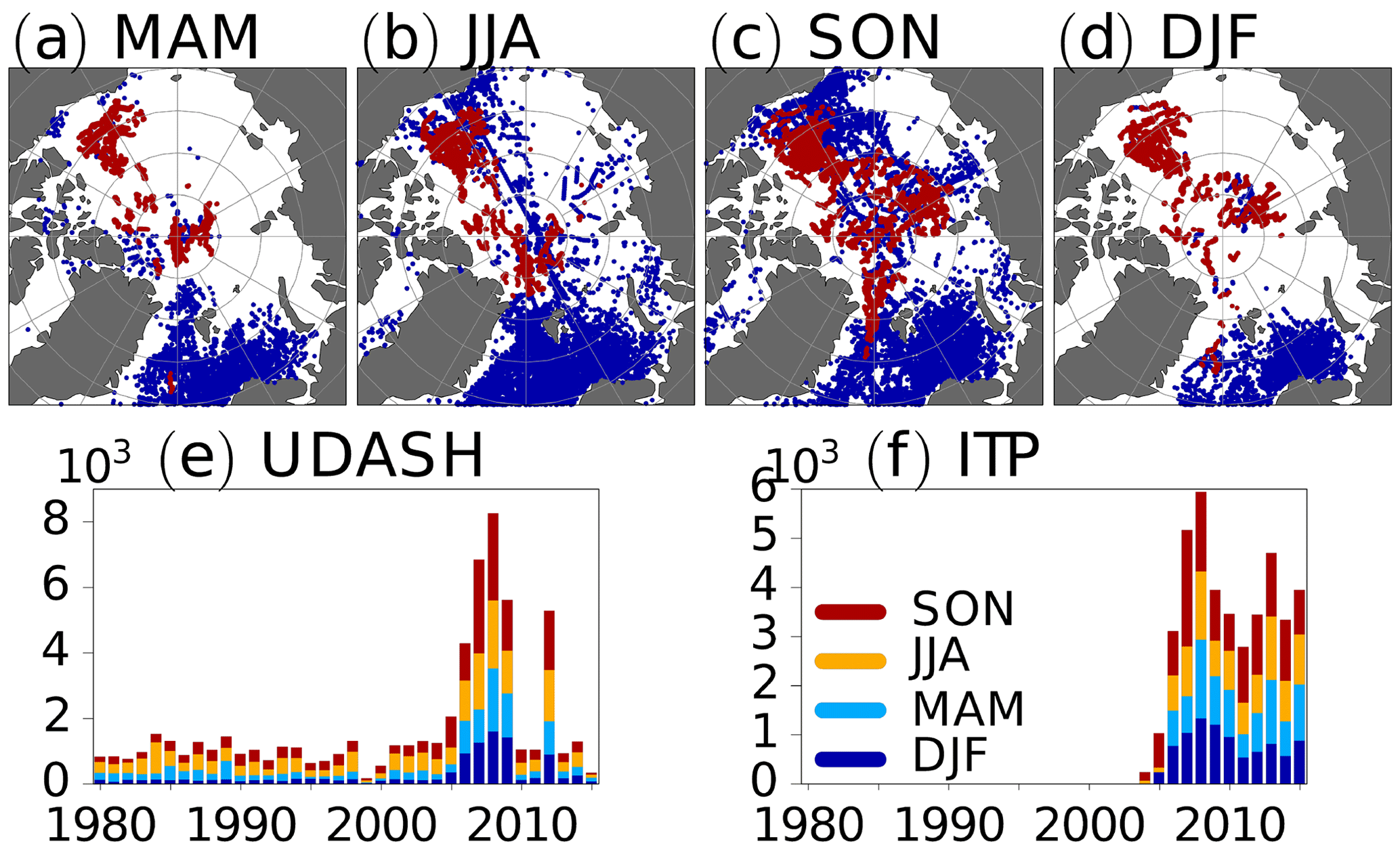
Figure 1Locations of observations for each season (starting with MAM for March, April, and May) with blue dots for UDASH profiles and red dots for ITP profiles (a–d). Temporal coverage for UDASH (e) and ITP (f) observations.

Depth was computed from pressure using the hydrostatic equation. Density was computed based on salinity, temperature, and pressure. In order to reduce noise, S, T, and/or θ were smoothed using a standard one-dimensional Gaussian filter (convolution with a Gaussian function; e.g., Deng and Cahill, 1993) with a standard deviation of 2 dbar and a truncation at ±10 dbar. When using thresholds to estimate the SML or CHL base depth, variables were linearly interpolated between two adjacent depths. Consequently, the SML or CHL base can be located between two vertical observation points and the SML and CHL base depths do not necessarily have to coincide with the depths of the observations.

3.1 Comparison of methods for deriving halocline base depth using case studies

Figure 2 compares three different methods for determining the halocline base depth for ITP-74. Starting from the Laptev Sea in September 2013, ITP-74 drifted across the central Arctic, almost reaching the East Greenland Sea (Fig. 2a). Fig. 2b–d shows evidence of a well-defined and stably stratified CHL below the SML until May 2014. The vertical stratification observed by ITP-74 prior to May 2014 and the performance of the three methods for determining the halocline base depth are further analyzed in an individual profile from this period in Fig. 3. Supplement 4 shows a corresponding figure based on Level I data instead of the more processed Level III data and equations from McDougall et al. (2010) instead of Gill (1982). Supplement 5 shows the locations of the profiles analyzed in Fig. 3 together with maps of sea ice concentration based on Spreen et al. (2008).

Individual profiles of salinity and temperature for 13 January 2014 in Fig. 3a show the base of the SML at about ∼ 30 m. Between the SML base and ∼ 80 m, a strong salinity gradient and temperatures close to the freezing point indicate a well-defined CHL, which is ∼ 60 m thick. Between the CHL and the AW, temperature and salinity increase in the LHW. Below ∼ 170 m, warm and saline AW is found (please note the kink in the temperature and salinity profiles at ∼ 170 m in Fig. 3a). The potential density anomaly used to compute the SML base is shown in Fig. 3b. Figure 3c–e show the density ratio, the temperature difference, and the stability for the observations on 13 January 2014. Threshold values used to identify the halocline base with the DR, TD, and ST methods are also shown. For the profile observed on 13 January 2014, the DR method (Fig. 3c) and the ST method (Fig. 3e) identify the CHL base, while the TD method places the halocline base in the LHW, somewhere between CHL and AW (Fig. 3c). The stability profile in Fig. 3d yields distinctly different stabilities for the SML, the CHL, the LHW, and the AW. A caveat is that observations are known to show spurious salinity extremes in high-gradient segments because of different sensitivity and time constants of temperature and conductivity sensors (e.g., Johnson et al., 2007). This can have consequences for the application of the methods. For example, the DR method may select density ratio values affected by the spurious salinity extremes. Although Level 3 ITP data (processed data applying sensor corrections) were used here, it is possible that salinity profiles exhibit false extremes in areas with significant temperature and salinity gradients.

In May 2014, the SML deepens and the CHL disappears (Fig. 2), as previously noted by Polyakov et al. (2017). During this convection event, none of the three methods identified a halocline. Figure 3h–j show profiles for 20 May 2014 after the onset of convection. On this date, the threshold for identifying the halocline base had already been exceeded at the SML base for the DR and the TD methods (Fig. 3h and i), while the threshold had not been reached for the ST method (Fig. 3j). In July, the situation becomes particularly interesting. The stability at about 80 m depth remains low, pointing to the residual of a mixed layer well below the determined SML base (Fig. 2). Figure 3k for 15 July 2014 (after convection) also shows freshening and warming near the surface. This indicates that relatively fresh melt water or/and shelf water may have been advected above a colder and saline layer, which had previously been homogenized by winter convection. The freshening near the surface leads to a salinity gradient below and to a stability maximum. This stability maximum is captured by the ST method (Fig. 3o). This appears to be consistent with the convective homogenization and capping mechanism for halocline formation described by Rudels et al. (1996). Figure 2 suggests that in this particular case, the convection may have affected halocline water because of the well-defined halocline prior to the onset of convection. This is also consistent with a study by Steele and Boyd (1998), who suggested that the winter convection and capping mechanism can act in addition to the advection of dense and saline shelf waters. In the Steele and Boyd (1998) mechanism, which combines findings by Rudels et al. (1996) with earlier findings (e.g., Aagaard et al., 1981), high salinity in the capped water derives from advected cold and dense shelf water, which may have previously been affected by brine release in shelf seas, and not directly from AW. Here, the origin of the halocline water is unclear. However, Fig. 3o for 15 July 2014 (after winter convection) identifies a stability maximum associated with fresh water near the surface. This suggests that the ST method might indeed be useful for identifying the beginning of new halocline formation via the Rudels et al. (1996, 2004) convective homogenization and capping mechanism or the Steele and Boyd (1998) mechanism, which essentially assumes that the Rudels et al. (1996) convective homogenization and capping mechanism acts in addition to the advection of dense shelf water (e.g., Aagaard et al., 1981).

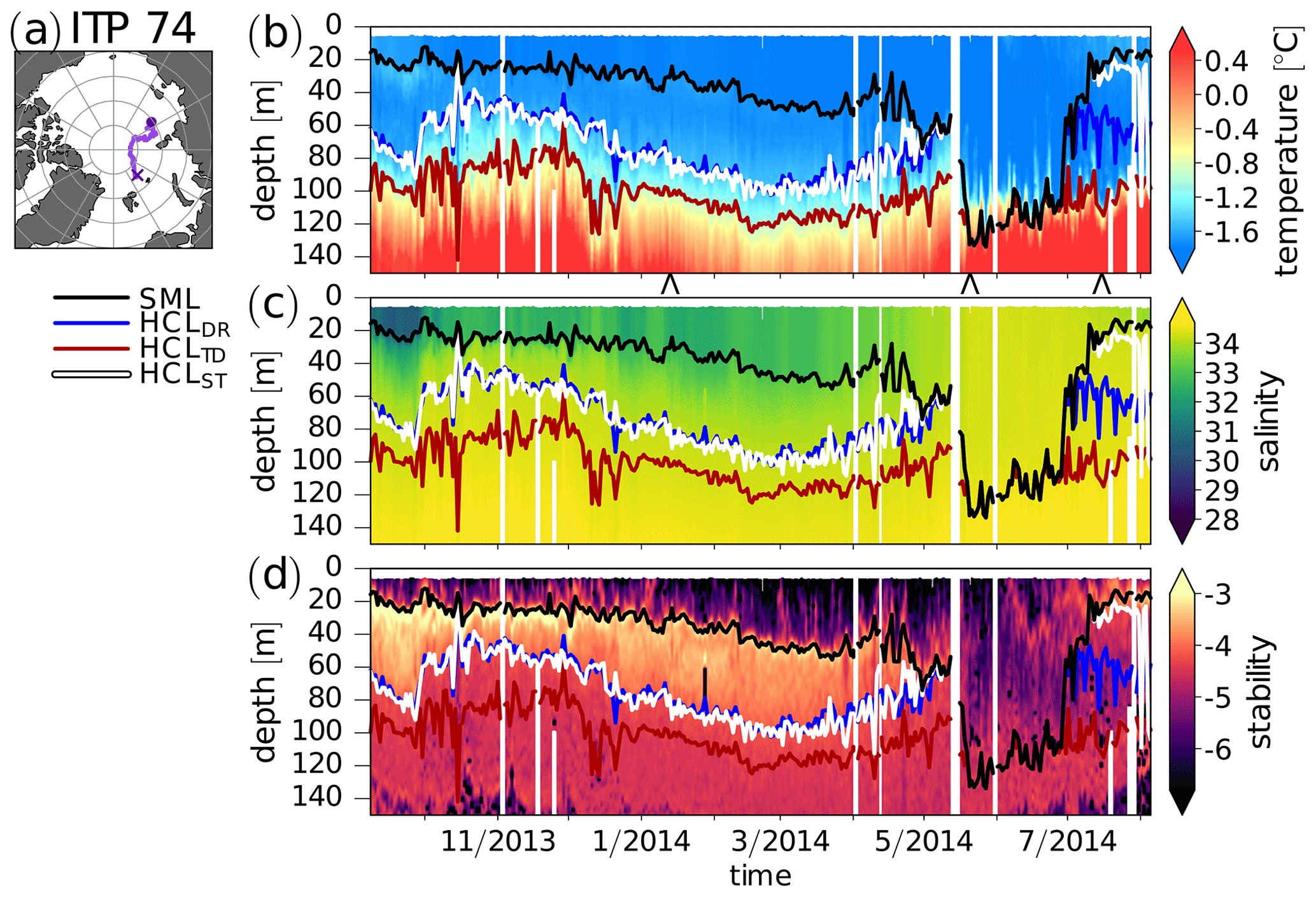
Figure 2ITP-74 location of measurements (a) and time series of temperature (b), salinity (on the practical salinity scale) (c), and vertical stability (L, unitless; see Sect. 2.1.3) (d). The circle and the cross in (a) mark the beginning and the end of the ITP-74 track, respectively. The colored lines in (b)–(d) are the base of the SML (black) and the halocline (HCL) base depths derived by the DR method (blue), the TD method (red), and the ST method (white). Individual profiles at the location of the wedge symbols (∧) below the x axis in (b) are shown in Fig. 3. Profiles that started below 15 m were not included in this figure (but were included everywhere else) because this increased readability by reducing the effect of noise in determining the SML base without affecting the overall result.

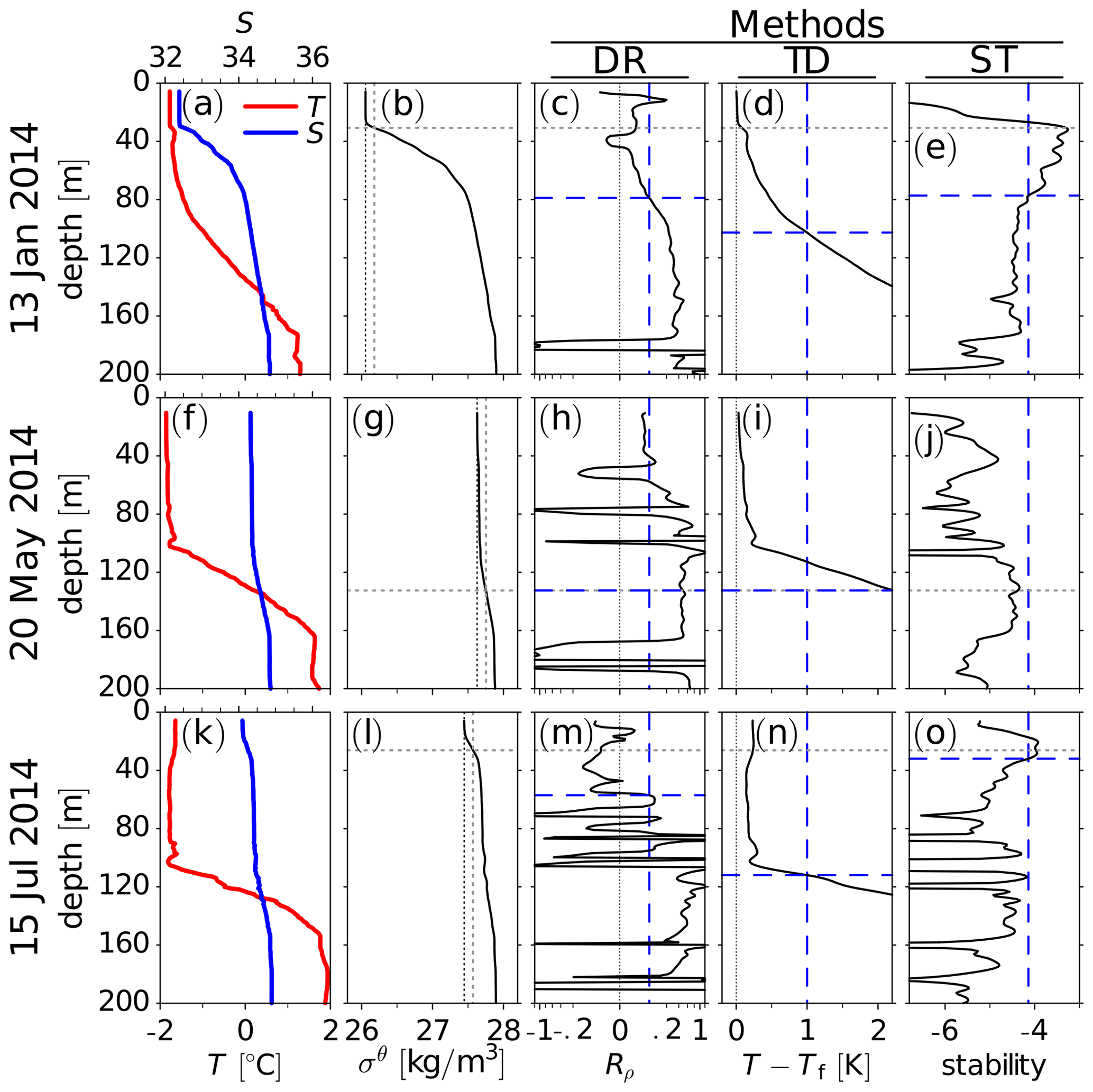
Figure 3Temperature T and salinity S (a, f, k), potential density anomaly ${\mathit{\sigma }}^{\mathit{\theta }}={\mathit{\rho }}^{\mathit{\theta }}-\mathrm{1000}$ kg m⁻³, where ρ^θ is potential density (b, g, l), density ratio R_ρ (please note the cubic scaling of the x axis) (c, h, m), temperature difference T−T_f, where T_f is the freezing temperature (d, i, n), and stability L (e, j, o) from ITP-74 before winter convection on 13 January 2014 (a–e), during winter convection on 20 May 2014 (f–j), and after winter convection on 15 July 2014 (k–o). Vertical dotted lines in (b), (g), and (l) indicate the surface density anomaly and the threshold for determining the SML base (i.e., surface density plus 0.125 kg m⁻³). Horizontal dotted lines indicate the SML base. Vertical dashed lines indicate threshold values for determining the halocline base. Horizontal dashed lines indicate the halocline base determined by the three different methods. Dashed lines overlying dotted lines in (h) and (i) indicate that a threshold for identifying the halocline base was exceeded at the SML base.

Download

Figure 4 again compares the three different methods for determining the halocline base depth but this time for ITP-33, which drifted into the Canada Basin between October 2009 and January 2011, where it encountered PSW on top of PWW. In addition to the halocline base depth, Fig. 4b–d shows the CHS boundaries which have been estimated based on stability as described above. The performance of the new algorithm for identifying the CHS will be discussed further below. For now, the main focus will be on isolated spurious minima of the halocline base depth. As evidenced by the spikes in Fig. 4b–d, such isolated spurious base depth minima occur for the DR and the TD algorithm but not the ST algorithm. Figure 5a–e shows a case from ITP-33 on 11 July 2010 in which the TD method produced an isolated halocline base depth minimum, and Fig. 5f–j shows a case on 6 September 2010 in which the DR method produced an isolated halocline base depth minimum. In both cases, the isolated minima are related to a layer of warm PSW around ∼ 80 m (Fig. 5a and f; see also Fig. 4b). For 11 July 2010, the best estimate of the halocline base depth is provided by the DR method (Fig. 5c). The DR method correctly places the base of the halocline water at a depth where the salinity gradient changes (Fig. 5a). Stability also decreases markedly at this depth, although the ST method identifies the halocline base about 20 m below this location (Fig. 5e). The TD method places the halocline base at about 80 m in the layer of warm PSW (Fig. 5d), although the salinity gradient below this layer still indicates the presence of a halocline and temperature decreases below this layer, indicating PWW. For 6 September 2010, the DR threshold is exceeded at a local density ratio maximum (Fig. 5h), which is related to a very steep temperature gradient at the base of the PSW (Fig. 5f). While all three methods rely on finding a threshold, the search direction differs. Because the ST method searches upward, the warm PSW layer does not result in isolated depth minima (Fig. 5e and j). Overall, this analysis suggests that the search direction is important regarding whether or not spurious halocline base depth minima are detected. With the DR and the TD method, we search downward, while with the ST method we search upward. Based on the stability profile in Fig. 5e, searching downward would lead to spurious depth minima in the ST method as well. This implies that the downward search direction in the ST method helps to explain why the ST method yields more robust results with fewer unexpected depth minima appearing in the basin-wise statistics discussed below. For the DR method, on the other hand, Fig. 3a shows that the DR threshold is exceeded also far below the halocline base. Such local DR maxima below the halocline base were also found in the presence of thermohaline staircases (not shown here). Additional DR maxima below the halocline base, such as the one in Fig. 3, prevent us from simply reversing the search direction in the DR algorithm.

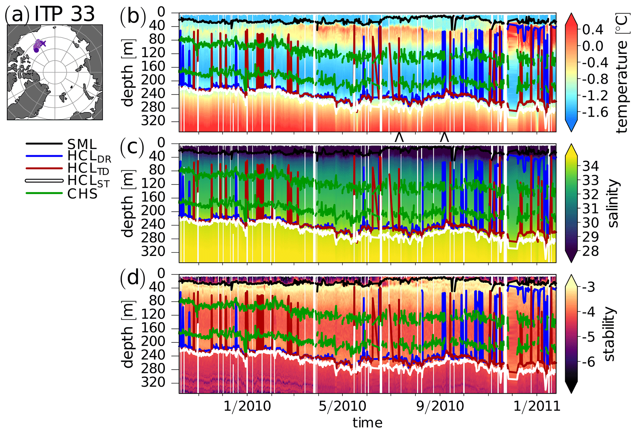
Figure 4As Fig. 2 but for ITP-33. Additionally, the results of the cold halostad bound estimation are shown in dark green.

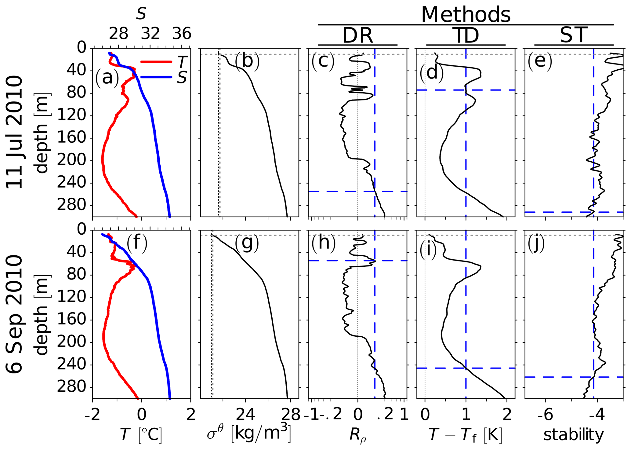
Figure 5As Fig. 3 but for two profiles from ITP-33. For 12 July 2010 (a–e) the TD method shows an isolated minimum of the halocline base depth, and for 6 September 2010 (f–j) the DR method shows an isolated minimum of the halocline base depth. Supplement 6 shows a corresponding figure based on Level I data instead of the more processed Level III data.

Download

3.2 Statistical comparison of the halocline base depth and occurrence frequency from different methods

In order to identify differences between the methods used for halocline base detection regarding the geographical distribution of halocline base depth and halocline occurrence frequency (i.e., the number of profiles for which a halocline base was detected divided by number of profiles analyzed), we used simple nearest-neighbor (NN) averaging to produce maps (Fig. 6). In addition to these maps (which in data-rich regions show a time mean halocline base depth), we computed basin-wise statistics of halocline base depths. Figure 7 shows relative frequencies of halocline base depths determined with the three methods for the Eurasian Basin, the Makarov Basin, and the Canada Basin.

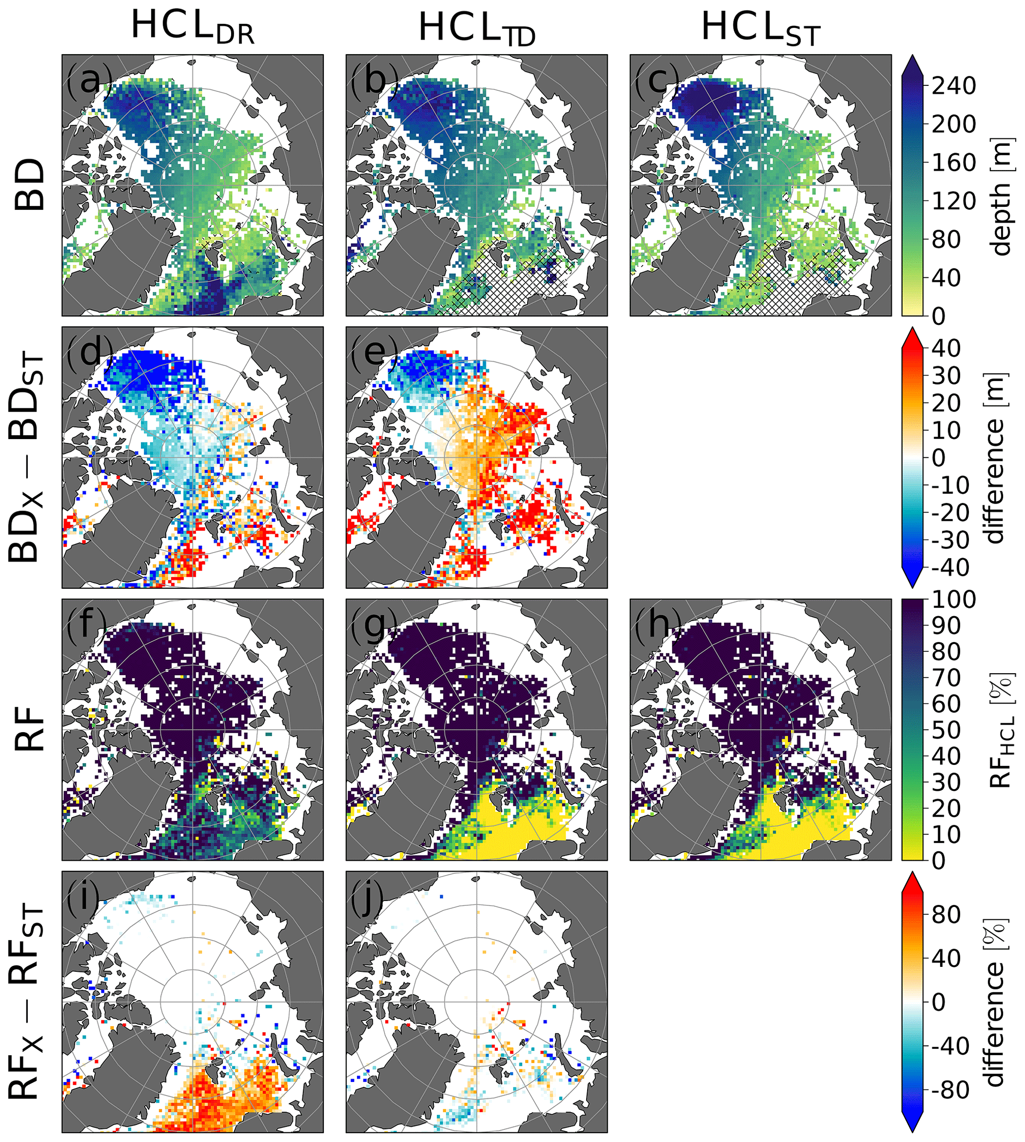
Figure 6Halocline (HCL) base depth (BD) derived by the density ratio (DR) algorithm (a), the temperature-difference (TD) algorithm (b), and the new stability (ST) algorithm (c). Difference in HCL BD between the DR and the ST algorithm (d) and between the TD and the ST algorithm (e). Relative frequency (RF) of HCL occurrence (i.e., the number of profiles for which a halocline was detected divided by number of profiles analyzed) (f–h) and differences (i–j) as in (a)–(e). In (a)–(c), points where the relative occurrence frequency of the HCL was below 1 % were masked out. Hatching indicates regions where the HCL occurrence frequency is below 25 %. Points where the ocean floor is shallower than 100 m were masked out.

As expected, all three methods yield a similar overall spatial distribution of halocline base depth with a shallower halocline base in the Eurasian Basin and the Makarov Basin compared to the Canada Basin (Fig. 6a–c). This spatial pattern is consistent with Polyakov et al. (2018). In the Eurasian Basin, the time-averaged halocline base depths determined with the DR method (Fig. 6a) and the ST method (Fig. 6c) agree relatively well, while the TD method placed the halocline at greater depth compared to the other methods (Fig. 6b). For the elliptical area covering the Eurasian Basin in Fig. 7a, the mean base depth was 85.9 m for the DR method and 92.3 m for the ST method vs. 116.1 m for the TD method. This greater halocline base depth from the TD method compared to the other two methods is consistent with the previous result for ITP-74. Unlike the DR and the ST methods, which both correctly identified the CHL base during the first months of ITP-74, the TD method placed the halocline base somewhere in the LHW.

In addition to the moderate difference in the mean base depth between the DR and the ST methods, the relative frequency of halocline base depth in the Eurasian Basin reveals differences between the DR and the ST methods that are not reflected by the difference in the mean base depths (Fig. 7b). The ST method more often identifies a shallow halocline base (< 60 m) in the Eurasian Basin compared to the DR method, which is consistent with the finding that the ST method apparently captures the start of new halocline formation from Sect. 3.1. The ST method also detects more frequent cases of halocline base depth below 120 m compared to the DR method (Fig. 7b). The more frequent halocline base depths larger than 120 m in the ST method are likely related to a deeper halocline base similar to the one found for the ST method for ITP-33 above. Slightly increasing the stability threshold in the ST method may lead to a better match between the halocline base depth estimate from the ST and the TD methods by moving the halocline base estimated by the ST method upward and by decreasing the sensitivity of the ST method to new halocline formation. For the elliptical area covering the Makarov Basin in Fig. 7b, the DR method yielded a mean halocline base depth of 112.3 m, the ST method 118.1 m, and the TD method again yielded a greater mean halocline base depth, 133.5 m.

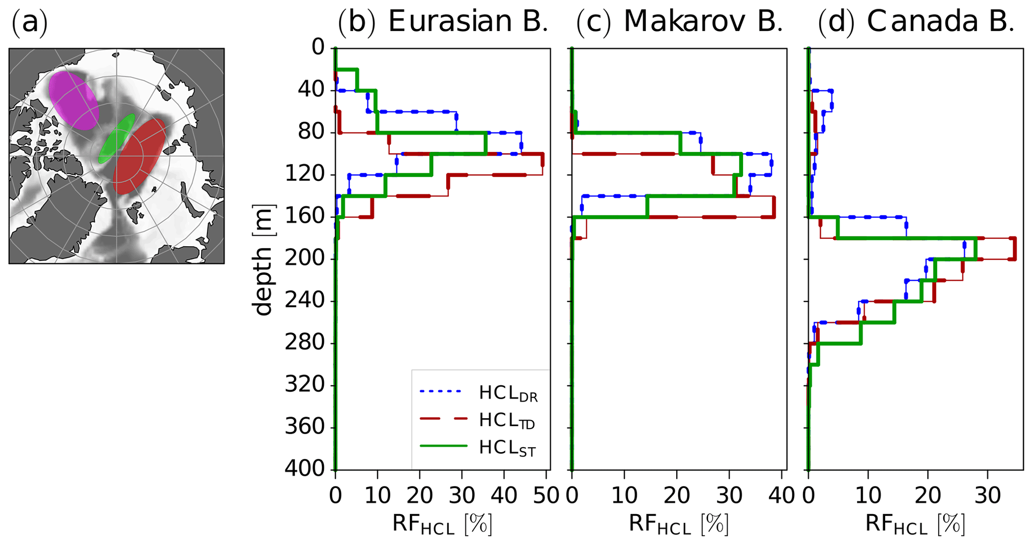
Figure 7Map showing elliptical areas over the Canada Basin (purple), the Makarov Basin (green), and the Eurasian Basin (dark red) and ocean floor depth (gray shading) (a). Relative frequency of halocline (HCL) base depth determined with the density ratio (DR), temperature difference (DR), and stability (ST) methods for the elliptical areas over the Eurasian Basin (b), the Makarov Basin (c), and the Canada Basin (d).

For the elliptical area covering the Canada Basin, on the other hand, the ST method yielded the largest mean halocline base depth. The mean halocline base depths for the Canada Basin corresponding to Fig. 7d are 191.4 m for the DR method, 206.6 m for the TD method, and 219.1 m for the ST method. In the Canada Basin, the ST method detected a halocline base shallower than 160 m for 0.05 % of the profiles, the DR method for 10.2 % of the profiles, and the TD method for 3.5 % of the profiles, the latter two values indicative of isolated base depth minima due to the influence of warm PSW above PWW (Fig. 7d). Isolated minima very likely also contribute to a more variable (noisier) halocline base depth in the Canada Basin in the map for the DR method in Fig. 6a and to a lesser extent also in the map for the TD method in Fig. 6b compared to the ST method (Fig. 6c). The greater average base depth in the Canada Basin in the ST method compared to the other methods (see also Fig. 6d and e) is, however, not only explained by the isolated depth minima in the DR and the TD methods in Fig. 7d; rather, more frequent depths greater than 260 m in the ST method compared to the two other methods (Fig. 7d) contribute to the greater average halocline base depth determined with the ST method. This again indicates that a slight increase in the stability threshold in the ST method would lead to better agreement between the halocline base depth from the ST and the DR methods. While a halocline was almost always detected in the Canada Basin by all three methods, the relative occurrence frequency (defined as the number of profiles in which a halocline base was detected divided by the total number of profiles which were analyzed) varies strongly in the Norwegian Sea (Fig. 6f–h). While the ST method and the TD methods very rarely detected a halocline base in the Norwegian Sea, the DR method frequently detected a halocline base in the Norwegian Sea. Furthermore, the DR method suggests a transition from a deeper halocline in relatively warm water inflow to a shallower halocline further north, which is absent in the other two methods (Fig. 6a–c). When using the DR method for analyzing halocline retreat in these warm water inflow regions, this may lead to different results compared to the two other methods. One reason for the DR method detecting a halocline base at depth could be thermohaline staircases. Overall, the largest differences in halocline detection frequency between the methods (Fig. 6i and j) were found in regions which are prone to sea ice retreat and, according to global climate model results, may also be particularly prone to events in which large temperature gradients are found directly underneath the SML and which mainly occur during winter (Metzner et al., 2020). In order to prevent the DR method from identifying a halocline base in relatively warm water, one could either limit the region to which the method is applied (as Polyakov et al., 2018) or else introduce additional constraints on the water temperature. Limiting the region is clearly a sensible choice in a stable climate. However, limiting the region to one in which a stable (cold) halocline is found at most times limits us in studying regional shifts. With regard to shifts due to climate change, one should be aware that methods differ regarding requirements for halocline base identification and results.

3.3 Estimation of cold halostad boundaries

In the Canada Basin, the PWW forms a cold halostad, while the LHW is modified water of Atlantic origin. This leads to a local vertical stability minimum between two local vertical stability maxima (Fig. 5e and j). The local minimum of vertical stability between these two local maxima is associated with a small salinity gradient around the core of the PWW (Fig. 5a and f). Top and base depth time series of the CHS derived with the new algorithm described in Sect. 2.2 are shown by dark green lines in Fig. 4. The algorithm was designed to avoid misclassifications of the cold halostad by requiring the difference between the lower stability maximum and the stability minimum (i.e., the depth of the “stability valley”) to be at least 0.2. Furthermore, the vertical extent of the stability valley was required to be greater than 50 m. This leads to occasional discontinuities in the cold halostad boundary. Figure 4 shows such discontinuities as evidenced by the breaks in the dark green lines. Furthermore, the requirement of a minimum depth leads to shallow halostad layers not being detected.

Collecting all available observations with detected cold halostad boundaries per grid cell leads to the maps of CHS center depth and CHS thickness shown in Fig. 8a and b. The main occurrence region of the cold halostad is the Canada Basin, where Pacific Water circulates between the SML and water of Atlantic origin (Shimada et al., 2005). Employing conservative assumptions to avoid a misclassification (including a lower bound of 50 m for the thickness), we detect a cold halostad layer in the Canada Basin region in Fig. 8b ∼ 70 %–90 % of the time, except in August, September, and October, when the mean occurrence frequency ranges from slightly below 60 % to slightly below 70 % (Fig. 8c). Figure 8a and b show that cold halostad was also detected to the northeast of Greenland, facing Svalbard from the west side of Fram Strait, where glacial cold water may act similar to the low-salinity Pacific Water (Dmitrenko et al., 2017).

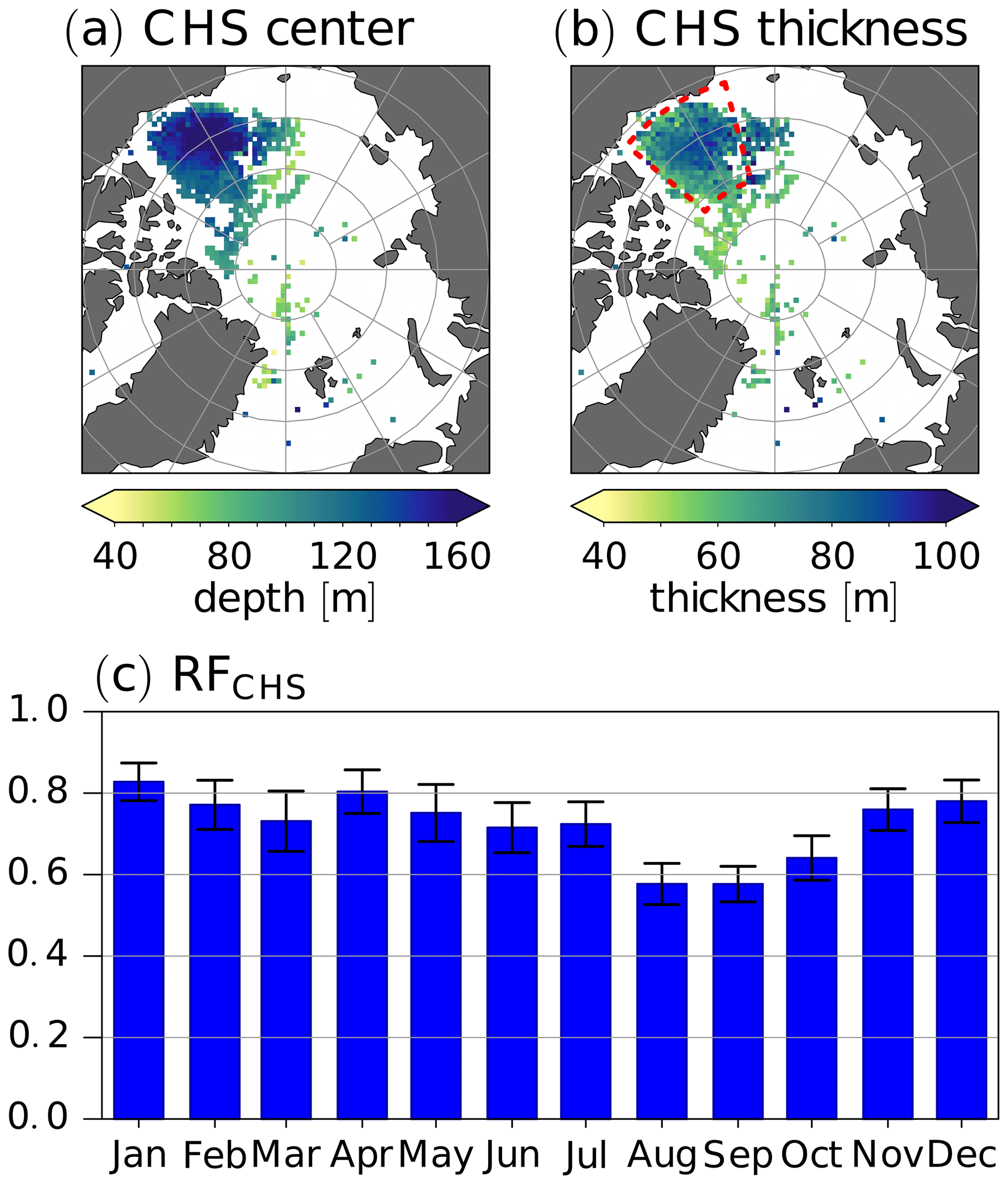
Figure 8Maps of mean CHS center depth (a) and CHS thickness (b). Monthly relative occurrence frequency (RF_CHS) of the CHS in the Canada Basin region (area enclosed by dashed red lines in (b)) and 95 % confidence interval for the mean (c).